Spatially-adaptive sensing in nonparametric regression

Abstract

While adaptive sensing has provided improved rates of convergence in sparse regression and classification, results in nonparametric regression have so far been restricted to quite specific classes of functions. In this paper, we describe an adaptive-sensing algorithm which is applicable to general nonparametric-regression problems. The algorithm is spatially-adaptive, and achieves improved rates of convergence over spatially-inhomogeneous functions. Over standard function classes, it likewise retains the spatial adaptivity properties of a uniform design.

1 Introduction

In many statistical problems, such as classification and regression, we observe data $Y_{1},Y_{2},\dots,$ where the distribution of each $Y_{n}$ depends on a choice of design point $x_{n}.$ Typically, we assume the $x_{n}$ are fixed in advance. In practice, however, it is often possible to choose the design points sequentially, letting each $x_{n}$ be a function of the previous observations $Y_{1},\dots,Y_{n-1}.$

We will describe such procedures as adaptive sensing, but they are also known by many other names, including sequential design, adaptive sampling, active learning, and combinations thereof. The field of adaptive sensing has seen much recent interest in the literature: compared with a fixed design, adaptive sensing algorithms have been shown to provide improvements in sparse regression (Iwen, 2009; Haupt et al., 2011; Malloy and Nowak, 2011b; Boufounos et al., 2012; Davenport and Arias-Castro, 2012) and classification (Cohn et al., 1994; Castro and Nowak, 2008; Beygelzimer et al., 2009; Koltchinskii, 2010; Hanneke, 2011). Recent results have also focused on the limits of adaptive sensing (Arias-Castro et al., 2011; Malloy and Nowak, 2011a; Castro, 2012).

In this paper, we will consider the problem of nonparametric regression, where we aim to estimate an unknown function $f:[0,1]\to\mathbb{R}$ from observations

$$Y_{n}\coloneqq f(x_{n})+\varepsilon_{n},\quad\varepsilon_{n}\overset{\mathrm{i.i.d.}}{\sim}N(0,\sigma^{2}).$$

While previous authors have also considered this model under adaptive sensing, their results have either been restricted to quite specific classes of functions $f,$ or have not provided improved rates of convergence (Faraway, 1990; Cohn et al., 1996; Hall and Molchanov, 2003; Castro et al., 2006; Efromovich, 2008).

In the following, we will describe a new algorithm for adaptive sensing in nonparametric regression. Our algorithm will be based on standard wavelet techniques, but with an adaptive choice of design points: we will aim to codify, in a meaningful way, the intuition that we should place more design points in regions where $f$ is hard to estimate.

While many such heuristics are possible, we would like to construct an algorithm with good theoretical justification; in particular, we will be interested in attaining improved rates of convergence. In general, however, it is known that in nonparametric regression, adaptive sensing cannot provide improved rates over standard classes of functions. Castro et al. (2006) prove such a result for $L^{2}$ loss; we will show the same is true locally uniformly.

In the following, we will argue that the fault here lies not with adaptive sensing, but rather with the functions considered. In the field of spatial adaptation, unknown functions are often assumed to be spatially inhomogeneous: they may be rougher, and thus harder to estimate, in some regions of space than in others. The seminal paper of Donoho and Johnstone (1994) provides examples, which we have reproduced in Figure 1; these mimic the kinds functions observed in imaging, spectroscopy and other signal processing problems.

Figure 1: Examples of spatially-inhomogeneous functions from Donoho and Johnstone (1994). Each function is scaled to have $\mathrm{sd}(f)=7.$

Previous work in this field has provided many fixed-design estimators with good performance over such functions (Donoho et al., 1995; Fan and Gijbels, 1995; Lepski et al., 1997; Donoho and Johnstone, 1998; Fan et al., 1999). With adaptive sensing, however, we can obtain further improvements: if we place more design points in regions where $f$ is rough, our estimates $\hat{f}_{n}$ will become more accurate overall.

To quantify this, we will need to introduce new classes describing spatially-inhomogeneous functions, over which our algorithm will be shown to obtain improved rates of convergence. While these classes are novel, they will be shown to contain quasi-all functions from standard classes in the literature. Furthermore, our algorithm will be shown to adaptively obtain near-optimal rates over both the new and standard function classes.

Smoothness classes similar to our own have arisen in the study of adaptive nonparametric inference (Picard and Tribouley, 2000; Giné and Nickl, 2010; Bull, 2012), and more generally also in the study of turbulence (Frisch and Parisi, 1980; Jaffard, 2000). As in those papers, we find that for complex nonparametric problems, the standard smoothness classes may be insufficient to describe behaviour of interest; by specifying our target functions more carefully, we can achieve more powerful results.

We might also compare this phenomenon to results in sparse regression, where good rates are often dependent on specific assumptions about the design matrix or unknown parameters (Fan and Lv, 2008; van de Geer and Bühlmann, 2009; Meinshausen and Bühlmann, 2010). As there, we can use the nature of our assumptions to provide insight into the kinds of problems on which we can expect to perform well.

We will test our algorithm by estimating the functions in Figure 1 under Gaussian noise. We will see that, by sensing adaptively, we can make significant improvements to accuracy; we thus conclude that adaptive sensing can be of value in nonparametric regression whenever the unknown function may be spatially inhomogeneous.

In Section 2, we describe our adaptive-sensing algorithm. In Section 3, we describe our model of spatial inhomogeneity, and show that adaptive sensing can lead to improved performance over such functions. In Section 4, we discuss the implementation of our algorithm, and provide empirical results. Finally, we provide proofs in Appendix A.

2 The adaptive-sensing algorithm

We now describe our adaptive-sensing algorithm in detail. We first discuss how we estimate $f$ under varying designs; we then move on to the choice of design itself.

2.1 Estimation under varying designs

Given observations $Y_{1},\dots,Y_{n}$ at a set of design points $\xi_{n}\coloneqq\{x_{1},\dots,x_{n}\},$ we will estimate the function $f$ using the technique of wavelet thresholding, which is known to give spatially-adaptive estimates (Donoho and Johnstone, 1994). To begin, we will need to choose our wavelet basis; for $j_{0}\in\mathbb{N},$ let

$$\varphi_{j,k}\text{ and }\psi_{j,k},\quad j,k\in\mathbb{Z},\ j\geq j_{0},\ 0\leq k<2^{j},$$

be a compactly-supported wavelet basis of $L^{2}([0,1]),$ such as the construction of Cohen et al. (1993).

In the following, we will assume the wavelets $\psi_{j,k}$ have $N\in\mathbb{N}$ vanishing moments,

$$\int x^{n}\psi_{j,k}(x)\ dx=0,\quad n\in\mathbb{Z},\ 0\leq n<N,$$

and both $\varphi_{j,k}$ and $\psi_{j,k}$ are zero outside intervals $S_{j,k}$ of width $2^{-j}(2L-1),$

$$S_{j,k}\coloneqq 2^{-j}[k-L+1,k+L)\cap[0,1).$$

For any $i\in\mathbb{N},\ i\geq j_{0},$ we may then write an unknown function $f\in L^{2}([0,1])$ in terms of its wavelet expansion,

$$f=\sum_{k=0}^{2^{i}-1}\alpha_{i,k}\varphi_{i,k}+\sum_{j=i}^{\infty}\sum_{k=0}^{2^{j}-1}\beta_{j,k}\psi_{j,k},$$

and estimate $f$ in terms of the coefficients $\alpha_{j_{0},k},\beta_{j,k}.$

When the design is uniform, we can estimate these coefficients efficiently in the standard way, using the fast wavelet transform (Donoho and Johnstone, 1994). Suppose, as will always be the case in the following, that the design points $x_{n}$ are distinct, so we may denote the observations $Y_{n}$ as $Y(x_{n}).$ Given $i\in\mathbb{N},\ i\geq j_{0},$ suppose also that we have observed $f$ on a grid of design points $2^{-i}k,\ k\in\mathbb{Z},\ 0\leq k<2^{i}.$

We may then estimate the scaling coefficients $\alpha_{i,k}$ of $f$ as

$$\hat{\alpha}^{i}_{i,k}\coloneqq 2^{-\frac{i}{2}}Y(2^{-i}k),$$

since for $i$ large,

$$\alpha_{i,k}=\int_{S_{i,k}}f(x)\varphi_{i,k}(x)\ dx\approx 2^{-\frac{i}{2}}f(2^{-i}k).$$ (1)

By an orthogonal change of basis, we can produce estimates $\hat{\alpha}_{j_{0},k}^{i}$ and $\hat{\beta}_{j,k}^{i}$ of the coefficients $\alpha_{j_{0},k}$ and $\beta_{j,k},$ given by the relationship

$$\sum_{k=0}^{2^{j_{0}}-1}\hat{\alpha}^{i}_{j_{0},k}\varphi_{j_{0},k}+\sum_{j=j_{0}}^{i-1}\sum_{k=0}^{2^{j}-1}\hat{\beta}^{i}_{j,k}\psi_{j,k}\coloneqq\sum_{k=0}^{2^{i}-1}\hat{\alpha}^{i}_{i,k}\varphi_{i,k}.$$ (2)

These estimates can be computed efficiently by applying the fast wavelet transform to the vector of values $2^{-\frac{i}{2}}Y(2^{-i}k).$

Since we will be considering non-uniform designs, this situation will often not apply directly. Many approaches to applying wavelets to non-uniform designs have been considered in the literature, including transformations of the data, and design-adapted wavelets (see Kerkyacharian and Picard, 2004, and references therein). In the following, however, we will use a simple method, which allows us to simultaneously control the accuracy of our estimates for many different choices of design.

To proceed, we note that the value of an estimated coefficient $\hat{\alpha}^{i}_{j,k}$ or $\hat{\beta}^{i}_{j,k}$ depends only on observations $Y(x)$ at points $x\in S_{j,k}\cap 2^{-i}\mathbb{Z}.$ We may therefore estimate the wavelet coefficients $\alpha_{j_{0},k}$ and $\beta_{j,k}$ by

$$\hat{\alpha}_{j_{0},k}\coloneqq\hat{\alpha}_{j_{0},k}^{i_{n}(j_{0},k)}\qquad\text{and}\qquad\hat{\beta}_{j,k}\coloneqq\hat{\beta}_{j,k}^{i_{n}(j,k)},$$ (3)

where the indices $i_{n}(j,k)$ are chosen so that these estimates use as many observations as possible,

$$i_{n}(j,k)\coloneqq\max\left\{i\in\mathbb{N}:i>j,\ S_{j,k}\cap 2^{-i}\mathbb{Z}\subseteq\xi_{n}\right\}.$$ (4)

To ease notation, for now we will estimate coefficients only up to a maximum resolution level ${j_{n}^{\max}}\in\mathbb{N},$ ${j_{n}^{\max}}>j_{0},$ chosen so that $2^{j_{n}^{\max}}\sim n/\log(n).$ We will then be able to guarantee that the set in (4) is non-empty.

Using these estimates directly will lead to a consistent estimate of $f,$ but one converging very slowly; to obtain a spatially-adaptive estimate, we must use thresholding. We fix $\kappa>1,$ and for

$$e_{n}(j,k)\coloneqq\sigma 2^{-\frac{1}{2}i_{n}(j,k)}\sqrt{2\log(n)},$$ (5)

define the hard-threshold estimates

$$\hat{\beta}_{j,k}^{T}\coloneqq\begin{cases}\hat{\beta}_{j,k},&\lvert\hat{\beta}_{j,k}\rvert\geq\kappa e_{n}(j,k),\\ 0,&\mathrm{otherwise}.\end{cases}$$

We then estimate $f$ by

$$\hat{f}_{n}\coloneqq\sum_{k=0}^{2^{j_{0}}-1}\hat{\alpha}_{j_{0},k}\varphi_{j_{0},k}+\sum_{j=j_{0}}^{{j_{n}^{\max}}-1}\sum_{k=0}^{2^{j}-1}\hat{\beta}_{j,k}^{T}\psi_{j,k}.$$ (6)

Given a uniform design $\xi_{n}=2^{-i}\mathbb{Z}\cap[0,1),$ this is a standard hard-threshold estimate; otherwise it gives a generalisation to non-uniform designs.

2.2 Adaptive design choices

So far, we have only discussed how to estimate $f$ from a fixed design. However, we can also use these estimates to choose the design points adaptively. We will choose the design points in stages, at stage $m$ selecting points $x_{n_{m-1}+1}$ to $x_{n_{m}}$ in terms of previous observations $Y_{1},\dots,Y_{n_{m-1}}.$ The number of design points in each stage can be chosen freely, subject only to the conditions that $n_{0}$ is a power of two, and the ratios $n_{m}/n_{m-1}$ are bounded away from 1 and $\infty.$ We may, for example, choose

$$n_{m}\coloneqq\lfloor 2^{j+\tau m}\rfloor,$$ (7)

for some $j\in\mathbb{N},$ and $\tau>0.$

In the initial stage, we will choose $n_{0}$ design points spaced uniformly on $[0,1],$

$$x_{i}\coloneqq(i-1)/n_{0},\quad 1\leq i\leq n_{0}.$$

At further stages $m\in\mathbb{N},$ we will construct a target density $p_{m}$ on $[0,1],$ and then select design points $x_{n_{m-1}+1},\dots,x_{n_{m}}$ so that the design $\xi_{n_{m}}$ approaches a draw from this density. We will choose $p_{m}$ to be concentrated in regions of $[0,1]$ where we believe the function $f$ is difficult to estimate, ensuring that later design points will adapt to the unknown shape of $f.$

At time $n_{m-1},$ for each $j\in\mathbb{N},\ j_{0}\leq j<{j_{n_{m-1}}^{\max}},$ we rank the $2^{j}$ thresholded estimates $\hat{\beta}^{T}_{j,k}$ in decreasing order of size. We then have

$$\left\lvert\hat{\beta}^{T}_{j,r_{j}^{-1}(1)}\right\rvert\geq\dots\geq\left\lvert\hat{\beta}^{T}_{j,r_{j}^{-1}(2^{j})}\right\rvert,$$

for a bijective ranking function $r_{j}.$ We will choose the target density so that, in the support of each significant term $\beta_{j,k}\psi_{j,k}$ in the wavelet series, the density will be, up to log factors, at least $2^{j}/r_{j}(k).$ The density will thus be concentrated in regions where the wavelet coefficients are known to be large. To ensure that all coefficients are estimated accurately, we will also require the density to be bounded below by a fixed constant, given by a choice of parameter $\lambda>0.$

Split the interval $[0,1]$ into sub-intervals

$$I_{l,m}\coloneqq 2^{-{j_{n_{m}}^{\max}}}[l,l+1),\quad l\in\mathbb{Z},\ 0\leq l<2^{j_{n_{m}}^{\max}}.$$

We define the target density on $I_{l,m}$ to be

$$p_{l,m}\coloneqq A\max\bigg{(}\left\{\lambda\right\}\cup\\ \left\{\frac{2^{j}}{r_{j}(k)({j_{n_{m-1}}^{\max}})^{2}}:j\in\mathbb{N},\ j_{0}\leq j<{j_{n_{m-1}}^{\max}},\ I_{l,m}\subseteq S_{j,k},\ \hat{\beta}^{T}_{j,k}\neq 0\right\}\bigg{)},$$

where the fixed constant $A>0$ is chosen so that the density $p_{m}$ always integrates to at most one, $2^{-{j_{n_{m}}^{\max}}}\sum_{l}p_{l,m}\leq 1.$ The specific value of $A$ is unimportant, but note that

$$2^{-{j_{n_{m}}^{\max}}}\sum_{l=0}^{2^{j_{n_{m}}^{\max}}-1}p_{l,m}\lesssim 1+({j_{n_{m-1}}^{\max}})^{-2}\sum_{j=0}^{j_{n_{m-1}}^{\max}}\sum_{k=1}^{2^{j}}k^{-1}\lesssim 1,$$

so such a choice of $A$ exists.

We now aim to choose new design points $x_{n_{m-1}+1},\dots,x_{n_{m}}$ so that the design $\xi_{n}$ approximates a draw from $p_{m}.$ To simplify notation, we first include any points $x\in 2^{-{j_{n_{m}}^{\max}}}\mathbb{Z}\cap[0,1)$ not already in the design. We will assume the $n_{m}$ and ${j_{n}^{\max}}$ are chosen so that this requires no more than $n_{m}-n_{m-1}$ design points; since ${j_{n}^{\max}}$ is defined only asymptotically, and $2^{{j_{n_{m}}^{\max}}}=o(n_{m}-n_{m-1}),$ such a choice is always possible.

We then construct an effective density $q_{m,n},$ describing a nominal density generating the design $\xi_{n}.$ This density will be at least $2^{i}/n$ on any region where the design contains the grid $2^{-i}\mathbb{Z};$ it will thus describe the density of all design points on regular grids. We define the effective density on $I_{l,m}$ at time $n$ to be

$$q_{l,m,n}\coloneqq n^{-1}\max\left\{2^{i}:i\in\mathbb{N},\ 2^{-i}\mathbb{Z}\cap I_{l,m}\subseteq\xi_{n}\right\}.$$

Again, note this density integrates to at most one, $2^{-{j_{n_{m}}^{\max}}}\sum_{l}q_{l,m,n}\leq 1.$

Our remaining goal is to choose the new design points so that the effective density approaches the target density. In our proofs, we will require control over the maximum discrepancy from $p_{m}$ to $q_{m,n},$

$$\max_{l=0}^{2^{j_{n_{m}}^{\max}}-1}p_{l,m}/q_{l,m,n}.$$ (8)

To choose the next stage of design points, having selected points $x_{1},\dots,x_{n},$ we therefore pick an $l$ maximising (8); note that this does not require us to calculate $A.$ We then add points $2^{-i}\mathbb{Z}\cap I_{l,m}$ to the design, choosing the smallest index $i$ for which at least one such point is not already present.

In doing so, we halve the largest value of $p_{l,m}/nq_{l,m,n},$ while leaving all other such values unchanged. Repeating this process, we will therefore add design points on grids $2^{-i}\mathbb{Z}\cap I_{l,m}$ so as to minimise (8). We continue until we have selected a total of $n_{m}$ design points; for convenience, let $q_{l,m}\coloneqq q_{l,m,n_{m}}$ denote the effective density on $I_{l,m}$ once we are done.

The final algorithm is thus described by Algorithm 1; it can be implemented efficiently using a priority queue to find values of $l$ maximising (8). We will show that this algorithm ensures the final effective density $q_{m}$ is close to the target density $p_{m},$ and that estimates made under it are therefore spatially-adaptive for a wide variety of functions.

Algorithm 1 Spatially-adaptive sensing

  $n\leftarrow n_{0}$

  $x_{1},\dots,x_{n}\leftarrow n^{-1}\mathbb{Z}\cap[0,1)$

  observe $Y_{1},\dots,Y_{n}$

  $m\leftarrow 1$

  loop

     $x_{n+1},\dots,x_{n^{\prime}}\leftarrow 2^{-{j_{n_{m}}^{\max}}}\mathbb{Z}\cap[0,1)\setminus\xi_{n}$

     $n\leftarrow n^{\prime}$

     while $n<n_{m}$ do

        choose $l$ maximising $p_{l,m}/q_{l,m,n}$

        $S\leftarrow 2^{-i}\mathbb{Z}\cap I_{l,m}\setminus\xi_{n},$ for the smallest $i$ such that $S\neq\emptyset$

        repeat

           $n\leftarrow n+1$

           choose $x_{n}\in S$

           $S\leftarrow S\setminus\{x_{n}\}$

        until $S=\emptyset$ or $n=n_{m}$

     end while

     observe $Y_{n_{m-1}+1},\dots,Y_{n}$

     estimate $f$ by $\hat{f}_{n}$

     $m\leftarrow m+1$

  end loop

3 Theoretical results

We now provide theoretical results on the performance of our algorithm. We begin by defining the relevant function classes, then discuss our choice of functions considered; we conclude with our results on convergence rates.

3.1 Function classes

We first define the function classes we will consider in the following. We will assume we have a wavelet basis $\psi_{j_{0},k},\varphi_{j,k}$ satisfying the assumptions of Section 2.1; we can then describe any function $f\in L^{2}([0,1])$ by its wavelet series,

$$f=\sum_{k=0}^{2^{j_{0}}-1}\alpha_{j_{0},k}\varphi_{j_{0},k}+\sum_{j=j_{0}}^{\infty}\sum_{k=0}^{2^{j}-1}\beta_{j,k}\psi_{j,k}.$$

The smoothness of $f,$ and thus the ease with which it can be estimated, is determined by the size of the coefficients $\alpha_{j_{0},k},\beta_{j,k};$ $f$ is smooth, and easily estimated, when these coefficients are small. The smoothness of a function can be described in terms of its membership of standard function classes. While there are many such classes, in what follows we will be interested primarily in the Hölder and Besov scales (Härdle et al., 1998).

For $s\in\mathbb{N},$ the Hölder classes $C^{s}(M)$ contain all functions which are $s$-times differentiable, with value and derivatives are bounded by $M;$ the local Hölder classes $C^{s}(M,I)$ instead require this condition to hold only over an interval $I.$ These definitions can also be extended to non-integer $s,$ and given in terms of wavelet coefficients. We note that while the wavelet definitions are in general slightly weaker than the classical ones, this will not fundamentally affect our results in what follows.

Definition 1.

For $s\in(0,N),$ $M>0,$ and $I\subseteq[0,1],$ $C^{s}(M,I)$ is the class of functions $f\in L^{2}([0,1])$ satisfying

$$\max\left(2^{j_{0}\left(s+\frac{1}{2}\right)}\sup_{k:S_{j_{0},k}\subseteq I}\lvert\alpha_{j_{0},k}\rvert,\ \sup_{j=j_{0}}^{\infty}2^{j\left(s+\frac{1}{2}\right)}\sup_{k:S_{j,k}\subseteq I}\lvert\beta_{j,k}\rvert\right)\leq M.$$

For $I=[0,1],$ we denote this class $C^{s}(M).$

The Besov classes $B^{r}_{p,\infty}(M)$ are more general. For $p=\infty,$ they coincide with our definition of the Hölder classes $C^{r}(M).$ For $p<\infty,$ they allow functions with some singularities, provided they are still, on average, $r$-times differentiable; smaller values of $p$ correspond to more irregular functions.

Definition 2.

For $r\in(0,N),$ $p\in[1,\infty),$ and $M>0,$ $B^{r}_{p,\infty}(M)$ is the class of functions $f\in L^{2}([0,1])$ satisfying

$$\max\left(2^{j_{0}\left(r+\frac{1}{2}-\frac{1}{p}\right)}\left(\sum_{k}\lvert\alpha_{j_{0},k}\rvert^{p}\right)^{\frac{1}{p}},\ \sup_{j=j_{0}}^{\infty}2^{j\left(r+\frac{1}{2}-\frac{1}{p}\right)}\left(\sum_{k}\lvert\beta_{j,k}\rvert^{p}\right)^{\frac{1}{p}}\right)\leq M.$$

For $p=\infty,$ we define $B^{r}_{\infty,\infty}(M)\coloneqq C^{r}(M).$

Many other standard classes are related to these Besov classes, including the Sobolev classes $W^{r,p}(M)\subseteq B^{r}_{p,\infty}(M),$ the Sobolev Hilbert classes $H^{r}(M)\subseteq B^{r}_{2,\infty}(M),$ and the functions of bounded variation $BV(M)\subseteq B^{1}_{1,\infty}(M).$ In each case, convergence rates are unchanged by considering the containing Besov class, meaning we need consider only Besov classes in what follows.

Besov classes can also be thought of as describing functions whose wavelet expansions are sparse. From the above definitions, we can see that, compared to a Hölder class, functions in a Besov class can have a number of larger wavelet coefficients, provided there are not too many. In other words, functions in a Besov class can have wavelet expansions where most, but not all, coefficients are small.

Besov classes are often used to describe spatially-inhomogeneous functions; we can see why by considering Figure 2, which plots the wavelet coefficients of the functions in Figure 1. As above, the coefficients are often, but not always, small.

Figure 2: CDV-8 wavelet coefficients for the functions in Figure 1. The height of each line corresponds to a wavelet coefficient $\beta_{j,k};$ the $x$-axis plots the location $2^{-j}k,$ and the $y$-axis the scale $j.$

Our final function class is a new definition, which we will argue captures another typical feature of spatially-inhomogeneous functions, and is necessary to obtain improved rates of convergence. From Figure 2, we can see that, in regions where the functions $f$ are rough, their wavelet coefficients are often large; in regions where they are smooth, their coefficients are small. In other words, if $f$ is difficult to approximate in some region at high resolution, it will also be difficult to approximate there at lower resolutions.

We will call such functions detectable, and describe them in terms of detectable classes $D^{s}_{t}(M,I)\subseteq C^{s}(M,I).$ The additional parameter $t\in(0,1)$ controls the strength of our condition; larger $t$ corresponds to a stronger condition on functions $f.$

Definition 3.

For $s\in(0,N),$ $t\in(0,1),$ $M>0,$ and an interval $I\subseteq[0,1],$ $D^{s}_{t}(M,I)$ is the class of functions $f\in C^{s}(M,I)$ which also satisfy

$$\forall\ j\in\mathbb{N},\ j\geq\lceil\tfrac{j_{0}}{t}\rceil,\ k:S_{j,k}\cap I\neq\emptyset,\\ \exists\ j^{\prime}\in\mathbb{N},\ \lfloor tj\rfloor\leq j^{\prime}<j,\ k^{\prime}:S_{j^{\prime},k^{\prime}}\supset S_{j,k},\\ \lvert\beta_{j^{\prime},k^{\prime}}\rvert\geq(j^{\prime}/j)2^{(j-j^{\prime})\left(s+\frac{1}{2}\right)}\lvert\beta_{j,k}\rvert.$$ (9)

The definition thus requires that each term in the wavelet series on $I,$ at a fine scale $j,$ lies within the support of another term, of comparable size, at a coarser scale $j^{\prime}.$ The parameter $s$ controls how large this second term must be, and $t$ controls how far apart the scales $j$ and $j^{\prime}$ can be.

In Section 3.2, we will discuss why such conditions may be natural to consider for this problem. First, however, we will establish that a typical locally Hölder function will be detectable; indeed, similarly to results in Jaffard (2000) and Giné and Nickl (2010), we can show that the set of functions which are locally Hölder but not detectable is topologically negligible. We may therefore sensibly restrict to detectable functions in what follows.

Proposition 4.

For $s\in(0,N),$ $M>0,$ and any interval $I\subseteq[0,1],$ define

$$\mathcal{D}\coloneqq C^{s}(M,I)\setminus\bigcup_{t\in(0,1)}D^{s}_{t}(M,I).$$

Then $\mathcal{D}$ is nowhere dense in the norm topology of $C^{s}(M,I).$

3.2 Spatially-inhomogeneous functions

We now discuss our choice of functions to consider. We begin with some well-known results, which describe the limitations of adaptive sensing over Hölder classes. Let

$$\alpha(s)\coloneqq s/(2s+1),$$

and define an adaptive-sensing algorithm to be a choice of design points $x_{n}=x_{n}(Y_{1},\dots,Y_{n-1}),$ together with an estimator $\hat{f}_{n}=\hat{f}_{n}(Y_{1},\dots,Y_{n}).$ Then, up to log factors, a spatially-adaptive estimate can attain the rate $n^{-\alpha(s)}$ over any local Hölder class $C^{s}(M,I),$ and this cannot be improved upon by adaptive sensing.

Theorem 5.

Using a uniform design $x_{i}=(i-1)/n,$ there exists an estimator $\hat{f}_{n},$ which satisfies

$$\sup_{x\in J}\lvert\hat{f}_{n}(x)-f(x)\rvert=O_{p}(c_{n}),$$

uniformly over $f\in C^{s}(M,I)\cap C^{\frac{1}{2}}(M),$ for any $s\in[\frac{1}{2},N),$ $M>0,$ $I$ an interval open in $[0,1],$ $J\subseteq I$ a closed interval, and

$$c_{n}=(n/\log(n))^{-\alpha(s)}.$$

Theorem 6.

Let $s\geq\frac{1}{2},$ $M>0,$ $I$ an interval open in $[0,1],$ and $J\subseteq I$ a closed interval. Given an adaptive-sensing algorithm with estimator $\hat{f}_{n},$ if

$$\sup_{x\in J}\lvert\hat{f}_{n}(x)-f(x)\rvert=O_{p}(c_{n})$$

uniformly over $f\in C^{s}(M,I)\cap C^{\frac{1}{2}}(M),$ then

$$c_{n}\gtrsim n^{-\alpha(s)}.$$

To benefit from adaptive sensing, we will need to exploit two features of the functions in Figure 1. The first is that, as discussed in Section 3.1, these functions are sparse: they are rougher in some regions than others. This sparsity is necessary to benefit from adaptive sensing: it is the difference between rough and smooth which allows us to improve performance, placing more design points in rougher regions.

Sparsity is commonly measured in terms of Besov, rather than Hölder, classes. This change alone, however, is not enough to allow us to benefit from adaptive sensing. Since $B^{r}_{p,\infty}(M)\subseteq C^{r-1/p}(M),$ over this class we can achieve the rate $n^{-\alpha\left(r-1/p\right)},$ up to log factors, with the fixed-design method of Theorem 5. We can further show that, in this case, adaptive sensing offers little improvement.

Theorem 7.

Let $p\in[1,\infty],$ $r\geq\frac{1}{2}+\frac{1}{p},$ $M>0,$ and $I$ be an interval in $[0,1].$ Given an adaptive-sensing algorithm with estimator $\hat{f}_{n},$ if

$$\sup_{x\in I}\lvert\hat{f}_{n}(x)-f(x)\rvert=O_{p}(c_{n}),$$

uniformly over $f\in B^{r}_{p,\infty}(M),$ then

$$c_{n}\gtrsim n^{-\alpha\left(r-\frac{1}{p}\right)}.$$

To benefit from adaptive sensing, it is not enough to have regions in which the function is rough or smooth; we must also be able to detect where those regions are. This is the rationale behind our detectable classes $D^{s}_{t}(M,I)$: if a function is detectable, its roughness at high resolutions will be signalled by corresponding roughness at low resolutions, which we can observe in advance.

We will be interested in functions $f$ which are both sparse and detectable. For $p\in[1,\infty],$ $r\in[\frac{1}{2}+\frac{1}{p},N),$ $s\in[r-\frac{1}{p},N),$ $t\in(0,1),$ $M>0,$ and any interval $I\subseteq[0,1],$ let

$$\mathcal{F}=\mathcal{F}(p,r,s,t,M,I)\coloneqq B^{r}_{p,\infty}(M)\cap D^{s}_{t}(M,I)$$ (10)

denote a class of sparse and detectable functions.

We note that this class has two smoothness parameters: $r$ governs the average global smoothness of a function $f\in\mathcal{F},$ while $s$ governs its local smoothness over $I.$ Since functions in $B^{r}_{p,\infty}$ are everywhere at least $(r-\frac{1}{p})$-smooth, we have restricted to the interesting case $s\geq r-\frac{1}{p}.$

From 4, we know that quasi-all locally Hölder functions are detectable; we can likewise show that under a fixed design, restricting to sparse and detectable functions does not alter the minimax rate of estimation. We may thus conclude that requiring sparsity and detectability thus does not make estimation fundamentally easier.

Theorem 8.

Using a fixed design, if an estimator $\hat{f}_{n}$ satisfies

$$\sup_{x\in I}\lvert\hat{f}_{n}(x)-f(x)\rvert=O_{p}(c_{n}),$$

uniformly over $f\in\mathcal{F},$ then

$$c_{n}\gtrsim(n/\log(n))^{-\alpha(s)}.$$

3.3 Benefits of adaptive sensing

With adaptive sensing, however, we can take advantage of these conditions to obtain improved rates of convergence. We even can show that Algorithm 1 achieves this without knowledge of the class $\mathcal{F};$ we can thus adapt not only to the regions where $f$ is rough, but also to the overall smoothness and sparsity of $f.$

Theorem 9.

Algorithm 1 satisfies

$$\sup_{x\in I}\lvert\hat{f}_{n}(x)-f(x)\rvert=O_{p}(c_{n}),$$

uniformly over $f\in\mathcal{F},$ for $u\coloneqq\max(r-s,0),$

$$r^{\prime}\coloneqq s+tu,\qquad s^{\prime}\coloneqq s/(1-ptu),$$ (11)

and

$$c_{n}\coloneqq\left(n/\log(n)^{3}\right)^{-\alpha\left(\min(r^{\prime},s^{\prime})\right)}\log(n)^{1(r^{\prime}=s^{\prime})}.$$ (12)

We thus obtain, up to log factors, the weaker of the two rates $n^{-\alpha(r^{\prime})}$ and $n^{-\alpha(s^{\prime})}.$ Both of these rates are at least as good as the $n^{-\alpha(s)}$ bound faced by a fixed design; when $s<r,$ and the function $f$ may be locally rough, the rates are strictly better. In that case, we obtain the $n^{-\alpha(r^{\prime})}$ rate when $s/r\geq(1-t)/(2-t),$ and the $n^{-\alpha(s^{\prime})}$ rate otherwise.

The improvement is driven by two parameters: $t,$ which governs how easy it is to detect irregularities of $f,$ and $u,$ which governs how much rougher $f$ is locally than on average. When both $t$ and $u$ are large, the rates we obtain are significantly improved; in the most favourable case, when $u=1,$ and $t\approx 1,$ this result is equivalent to gaining an extra derivative of $f.$ We can even show that these rates are near-optimal over classes $\mathcal{F}.$

Theorem 10.

Given an adaptive-sensing algorithm with estimator $\hat{f}_{n},$ if

$$\sup_{x\in I}\lvert\hat{f}_{n}(x)-f(x)\rvert=O_{p}(c_{n}),$$

uniformly over $f\in\mathcal{F},$ then

$$c_{n}\gtrsim n^{-\alpha(\min(r^{\prime},s^{\prime}))},$$

for $r^{\prime},s^{\prime}$ given by (11).

Furthermore, we also have that, even in the absence of sparsity or detectability, we still achieve the spatial adaptation properties of a fixed design. We may thus use our adaptive-sensing algorithm with the confidence that, even if $f$ is spatially homogeneous, we will not pay an asymptotic penalty.

Theorem 11.

Algorithm 1 satisfies

$$\sup_{x\in J}\lvert\hat{f}_{n}(x)-f(x)\rvert=O_{p}\left(c_{n}\right),$$

uniformly over $f\in C^{s}(M,I)\cap C^{\frac{1}{2}}(M),$ for any $s\in[\frac{1}{2},N),$ $M>0,$ $I$ an interval open in $[0,1],$ $J\subseteq I$ a closed interval, and

$$c_{n}\coloneqq\left(n/\log(n)\right)^{-\alpha(s)}.$$

4 Implementation and experiments

We now give some implementation details of Algorithm 1, and provide empirical results. Before we test the algorithm, we must describe how we compute $\hat{f}_{n},$ and choose the parameters governing the algorithm’s behaviour.

4.1 Estimating functions

For simplicity, in (6) we defined $\hat{f}_{n}$ in terms of wavelets only up to the resolution level ${j_{n}^{\max}}.$ While asymptotically this carries no penalty, in finite time we may do better by estimating all the wavelets for which we have available data. In other words, we use the estimate

$$\hat{f}_{n}\coloneqq\sum_{k=0}^{2^{j_{0}}-1}\hat{\alpha}_{j_{0},k}\varphi_{j_{0},k}+\sum_{j=j_{0}}^{\infty}\sum_{k=0}^{2^{j}-1}\hat{\beta}_{j,k}^{T}\psi_{j,k},$$ (13)

where for $j\geq{j_{n}^{\max}},$ if the set in (4) is empty, we let $i_{n}(j,k)\coloneqq-\infty,$ forcing $\hat{\beta}_{j,k}^{T}=0.$ We note that since there are finitely many design points, the sum in (13) must have finitely many non-zero terms.

To compute these estimates $\hat{f}_{n},$ we must convert the estimated coefficients $\hat{\alpha}_{j_{0},k},$ $\hat{\beta}_{j,k}^{T}$ back into function values $\hat{f}_{n}(x).$ For $i\in\mathbb{N},\ i\geq j_{0},$ to evaluate $\hat{f}_{n}$ at points $x=2^{-i}k,$ $k\in\mathbb{Z},\ 0\leq k<2^{i},$ we make the approximation

$$\hat{f}_{n}(2^{-i}k)\approx 2^{\frac{i}{2}}\hat{\alpha}^{T}_{i,k},$$ (14)

where the post-thresholding scaling coefficients $\hat{\alpha}^{T}_{i,k}$ are defined by

$$\sum_{k=0}^{2^{i}-1}\hat{\alpha}^{T}_{i,k}\varphi_{i,k}\coloneqq\hat{f}_{n}.$$

These can again be computed efficiently using the fast wavelet transform.

Given a uniform design, and predicting $f$ only at the design points, this is enough to give estimates $\hat{f}_{n};$ if we set $\kappa=1,$ we have just described a standard hard-threshold wavelet estimate (Donoho and Johnstone, 1994). In that case, the observations and predictions are always made at the same scale, $i_{n}(j,k)=i,$ so the errors in (1) and (14) tend to cancel out. In other cases, however, the observations and predictions may be at different scales; these errors then may build up, making $\hat{f}_{n}$ look like a translation of $f.$

To resolve the issue, we will use a slightly different definition of the estimated coefficients $\hat{\alpha}_{j_{0},k}$ and $\hat{\beta}_{j,k},$ which ensures the scales of observation and prediction are the same. Given $i\in\mathbb{N},\ i\geq j_{0},$ to estimate $f$ at points $x=2^{-i}k,$ $k\in\mathbb{Z},\ 0\leq k<2^{i},$ we set $x_{n,k}\coloneqq\sup\{x\in\xi_{n}:x\leq 2^{-i}k\},$ and let

$$\hat{\alpha}_{i,k}\coloneqq 2^{-\frac{i}{2}}Y(x_{n,k}).$$

We then define the estimates $\hat{\alpha}_{j_{0},k}$ and $\hat{\beta}_{j,k}$ by

$$\sum_{k=0}^{2^{j_{0}}-1}\hat{\alpha}_{j_{0},k}\varphi_{j_{0},k}+\sum_{j=j_{0}}^{i-1}\sum_{k=0}^{2^{j}-1}\hat{\beta}_{j,k}\psi_{j,k}\coloneqq\sum_{k=0}^{2^{i}-1}\hat{\alpha}_{i,k}\varphi_{i,k},$$

using the fast wavelet transform as before.

We note that this definition is approximately the same as the one in (3); while it is harder to control theoretically, it gives improved experimental behaviour. We also note that, with a uniform design, if we wish to predict $f$ only at the design points, this again reduces to a standard wavelet estimate.

4.2 Choosing parameters

To apply Algorithm 1, we must choose the parameters $\kappa,$ $\lambda$ and $\tau,$ and also estimate $\sigma$ if it is not already known. The parameter $\kappa$ governs the size of our wavelet thresholds: larger $\kappa$ means we will be more conservative. While our theoretical results are proved for choices $\kappa>1,$ in our empirical tests we took $\kappa=1.$ This gives a simple choice of threshold which performs well, and allows us to compare our results with standard hard-threshold estimates.

The parameter $\lambda$ controls how uniform we make our design points: for $\lambda\gg 0$ the design points will be mostly uniform, while for $\lambda\approx 0$ they will be concentrated at irregularities of $f.$ The parameter $\tau$ likewise controls how many design points we choose at each stage: for $\tau\gg 0$ there will be a few large stages, while for $\tau\approx 0$ there will be many small ones. Empirically, we found the values $\lambda=\tau=\frac{1}{2}$ gave good trade-offs.

Finally, for uniform designs, Donoho and Johnstone (1994) suggest estimating $\sigma$ by the median size of the $\hat{\beta}_{j,k}$ at fine resolution scales. Our designs may not be uniform, but they are guaranteed to provide us with estimates $\hat{\beta}_{j,k}$ up to level ${j_{n}^{\max}}-1.$ We will therefore use the similar estimate

$$\hat{\sigma}_{n}\coloneqq\operatorname{median}\{2^{\frac{1}{2}i}\lvert\hat{\beta}_{j,k}\rvert:j\geq{j_{n}^{\max}}-1,i_{n}(j,k)>-\infty\}/0.6745,$$

which includes all estimated coefficients at scales at least this fine.

4.3 Empirical results

We now describe the results of using Algorithm 1 to estimate the functions in Figure 1, observing under $N(0,\sigma^{2})$ noise. Figure 3 plots $n=2^{11}$ noisy samples of each function, under a uniform design, with $\sigma=1,$ while Figure 4 plots a standard wavelet threshold estimate from these samples.

Figure 3: Noisy samples from the functions in Figure 1.

Figure 4: Fixed-design estimates of the functions in Figure 1.

Figure 5 plots typical results of using Algorithm 1 under these conditions. The algorithm was again given access to $n=2^{11}$ observations, with $\sigma=1;$ we set $n_{0}=2^{6},$ and chose the parameters $\kappa,\ \lambda,\ \tau,$ and $\hat{\sigma}_{n}$ as in Section 4.2. We used the family of wavelet bases described by Cohen et al. (1993), and implemented in Nason (2010); we took wavelets with $N=8$ vanishing moments, set $j_{0}=5,$ and ${j_{n}^{\max}}=\max(j_{0}+1,\lfloor n/\log(n)\rfloor).$

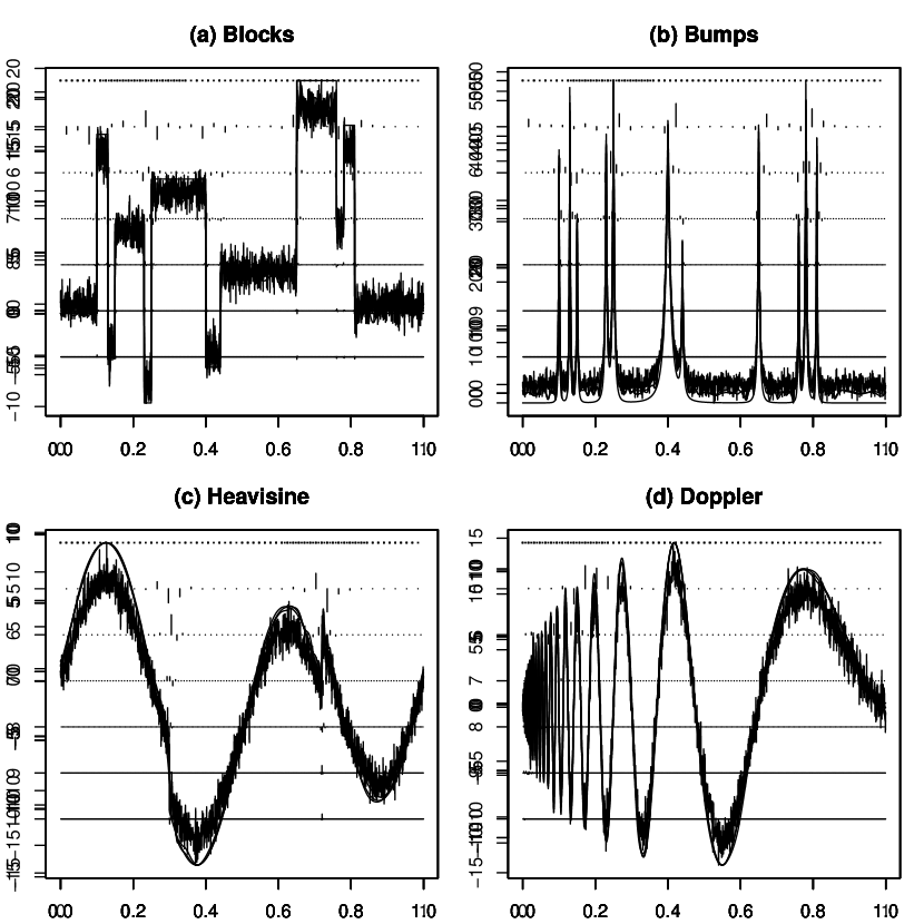
Figure 5: Adaptive-sampling estimates of the functions in Figure 1.

The dots along the top of each plot are drawn proportionally to the number of design points. We can see that, for the Heavisine and Doppler functions, the adaptive design concentrated in the regions where the function is rough; as a result, the adaptive estimates are noticeably better at recovering the shape of these curves.

For the Blocks and Bumps functions, which have more complicated patterns of spatial inhomogeneity, with these measurements the adaptive design was not able to locate all the areas where the functions are rough. However, we might expect performance on all the above functions to improve as the number of design points increases; to this end, we next considered performance with up to $n=2^{14}$ design points.

At this level of detail, it becomes harder to visually compare estimates; instead, to numerically measure the spatial adaptivity of our estimates, we evaluated procedures in terms of their maximum error over $[0,1],$ approximated by

$$\max_{x\in 2^{-j}\mathbb{Z}\cap[0,1)}\lvert\hat{f}_{n}(x)-f(x)\rvert$$

for $j$ large. In the following, we took $j=17,$ to avoid biasing the performance measure towards a uniform design.

Figure 6 compares the performance of the two methods on the Doppler function, with $\sigma=1;$ the values plotted are sample medians after 250 runs, together with 95% confidence intervals for the true median. We can see that for $n$ large, the adaptive design significantly outperforms the uniform one, consistent with a difference in the asymptotic rate of estimation.

Figure 6: Log-log plot of empirical performance on the Doppler function.

Table 1 compares performance on all the functions in Figure 1, given $n=2^{14}$ observations, and varying levels of $\sigma.$ We again report sample medians after 250 runs, together with the $p$-value of a two-sided Mann-Whitney-U test for difference in medians. (We note that the large errors reported for the Blocks function are due to the large discontinuities present, which are difficult to estimate uniformly over $[0,1].$)

	uniform design	adaptive design	$p$-value
$\sigma=0.5$
Blocks	13.284	13.3882	$<0.001$
Bumps	3.553	3.0086	$<0.001$
Heavisine	2.646	2.5902	$<0.001$
Doppler	1.783	0.5138	$<0.001$
$\sigma=1$
Blocks	12.355	12.799	$<0.001$
Bumps	5.721	5.487	$<0.001$
Heavisine	3.260	3.204	$<0.001$
Doppler	2.725	1.028	$<0.001$
$\sigma=2$
Blocks	11.121	10.988	0.428
Bumps	8.947	7.964	$<0.001$
Heavisine	3.053	3.061	0.815
Doppler	3.621	2.984	$<0.001$

Table 1: Empirical performance on the functions in Figure 1 for $n=2^{14}.$

We can see that for the Blocks function, the uniform design fared slightly better, as the adaptive algorithm still struggled to choose a good design. However, for the other three functions, adaptive sampling provided a significant improvement; the improvement was largest for small $\sigma,$ but still significant for two of the three functions even with large $\sigma.$ We thus conclude that adaptive sensing can be of value in nonparametric regression whenever the function $f$ may be spatially inhomogeneous.

Acknowledgements

We would like to thank Richard Nickl and several anonymous referees for their valuable comments and suggestions.

Appendix A Proofs

We now provide proofs of our results. We consider separately the results describing our detectability condition; the negative results, which establish lower bounds; and the constructive results, which control the performance of Algorithm 1.

A.1 Results on detectability

We now prove our first result, that detectability is a generic property of locally Hölder classes.

Proof of 4.

We will show any ball $B_{\varepsilon}(f)\subseteq C^{s}(M,I)$ contains a sub-ball $B_{\varepsilon/3}(f^{\prime})$ disjoint with $\mathcal{D}.$ Given $\varepsilon\in(0,M),$ and $f\in C^{s}(M,I)$ having wavelet coefficients $\alpha_{j_{0},k}$ and $\beta_{j,k},$ define a function $f^{\prime}$ with wavelet coefficients $\alpha_{j_{0},k}$ and $\beta_{j,k}^{\prime}$, where

$$\beta_{j,k}^{\prime}\coloneqq g\left(\beta_{j,k},\,\tfrac{2}{3}\varepsilon 2^{-j\left(s+\frac{1}{2}\right)}\right),$$

for

$$g(\beta,x)\coloneqq\begin{cases}x,&\beta\in[0,x],\\ -x,&\beta\in[-x,0),\\ \beta,&\text{otherwise.}\end{cases}$$

We then have $\lVert f-f^{\prime}\rVert_{C^{s}(I)}\leq\tfrac{2}{3}\varepsilon,$ so $B_{\varepsilon/3}(f^{\prime})\subset B_{\varepsilon}(f).$ Furthermore, every $\lvert\beta_{j,k}^{\prime}\rvert\geq\tfrac{2}{3}\varepsilon 2^{-j\left(s+\frac{1}{2}\right)},$ so for any function $f^{\prime\prime}\in B_{\varepsilon/3}(f^{\prime}),$ having wavelet coefficients $\alpha_{j_{0},k}^{\prime\prime}$ and $\beta_{j,k}^{\prime\prime},$ every $\lvert\beta_{j,k}^{\prime\prime}\rvert\geq\tfrac{1}{3}\varepsilon 2^{-j\left(s+\frac{1}{2}\right)}.$ Hence, for $t=\varepsilon/3M,$

$$\forall\ j\in\mathbb{N},\ j\geq\lceil\tfrac{j_{0}}{t}\rceil,\ k:S_{j,k}\cap I\neq\emptyset,\ j^{\prime}=\lfloor tj\rfloor,\ k^{\prime},\\ \lvert\beta_{j^{\prime},k^{\prime}}^{\prime\prime}\rvert\geq tM2^{-j^{\prime}\left(s+\frac{1}{2}\right)}\geq(j^{\prime}/j)2^{(j-j^{\prime})\left(s+\frac{1}{2}\right)}\lvert\beta_{j,k}^{\prime\prime}\rvert,$$

giving $f^{\prime\prime}\in D^{s}_{t}(M,I).$ ∎

A.2 Negative results

We begin our negative results by showing that, under a uniform design, restricting to sparse detectable functions does not alter the minimax rate of estimation. We will require Fano’s lemma, which relates the probability of misclassifying a signal to the Kullback-Leibler divergence between the alternatives (Tsybakov, 2009, §2.7.1). Given probability measures $\mathbb{P}$ and $\mathbb{Q}$ on $\mathbb{R}^{d},$ having densities $p$ and $q$ respectively, define the Kullback-Leibler divergence from $\mathbb{P}$ to $\mathbb{Q},$

$$D(\mathbb{P}\mid\mid\mathbb{Q})\coloneqq\int p(x)\log\left(\frac{p(x)}{q(x)}\right)dx.$$

Lemma 12 (Fano’s lemma).

Let $X\in\mathbb{R}^{d}$ have distribution $\mathbb{P}_{i},$ for some $i\in\mathbb{N},\ 1\leq i\leq k,$ and let $\psi(X)$ be an estimate of $i.$ Then

$$\sup\nolimits_{i}\mathbb{P}_{i}(\psi(X)\neq i)\geq 1-\frac{\beta+\log(2)}{\log(k-1)},$$

where

$$\beta\coloneqq\frac{1}{k^{2}}\sum_{i,j=1}^{k}D(\mathbb{P}_{i}\mid\mid\mathbb{P}_{j}).$$

We also make the definition

$$\lVert f\rVert_{I,\infty}\coloneqq\sup_{x\in I}\lvert f(x)\rvert,$$

for functions $f:[0,1]\to\mathbb{R},$ and $I\subseteq[0,1].$

Proof of Theorem 8.

The argument proceeds as a standard minimax lower bound; we construct functions $f_{n,k}\in\mathcal{F}$ a distance $c_{n}$ apart, and show we can only distinguish between them when $c_{n}\gtrsim(n/\log(n))^{-\alpha(s)}.$

Choose $j\in\mathbb{N}$ so that

$$2^{j}\sim(n/\log(n))^{1/(2s+1)},$$

and define a sequence $j_{1},\dots,j_{m}$ by

$$j_{m}\coloneqq j,\qquad j_{i-1}\coloneqq\lfloor tj_{i}\rfloor,\qquad j_{0}\leq j_{1}<\lceil\tfrac{j_{0}}{t}\rceil.$$

Since there are $n$ design points $x_{i},$ for $n$ large we must have an interval $S_{j_{m-1},k}\subseteq I$ containing $\lesssim 2^{-j_{m-1}}n$ of them; we will assume without loss of generality that this interval is always $S_{j_{m-1},0}.$ We then consider functions $f_{n,k}\in\mathcal{F},$ given by

$$f_{n,k}\coloneqq\sum_{i=1}^{m-1}M2^{-j_{i}\left(s+\frac{1}{2}\right)}\psi_{j_{i},0}+C2^{-j_{m}\left(s+\frac{1}{2}\right)}\psi_{j_{m},k},$$

where $k\in\mathbb{Z},\ 0\leq k<2^{j_{m}-j_{m-1}},$ and $C\in(0,M]$ is a constant to be determined.

Suppose $\lVert\hat{f}_{n}-f\rVert_{I,\infty}=O_{p}(c_{n}),$ uniformly over $\mathcal{F},$ for a sequence $c_{n}\not\gtrsim(n/\log(n))^{-\alpha(s)}.$ Then on a subsequence, we have $c_{n}=o\left((n/\log(n))^{-\alpha(s)}\right);$ passing to the subsequence, we may assume this is true for all $n.$ Since the $\psi_{j_{m},k}$ have distinct supports, for $n$ large we have

$$\min_{k\neq k^{\prime}}\lVert f_{n,k}-f_{n,k^{\prime}}\rVert_{I,\infty}\gtrsim C2^{-j_{m}s}\gtrsim C(n/\log(n))^{-\alpha(s)}.$$

Thus for $n$ large, $\hat{f}_{n}$ can distinguish between the $f_{n,k}$ with arbitrarily high probability. Let $\mathbb{P}_{k}$ denote the distribution of the observations when $f=f_{n,k};$ then any estimate

$$\hat{k}_{n}\coloneqq\underset{k}{\arg\min}\lVert\hat{f}_{n}-f_{n,k}\rVert_{\infty}$$

of $k$ satisfies

$$\sup_{k}\mathbb{P}_{k}(\hat{k}_{n}\neq k)\to 0$$

as $n\to\infty.$

However, for $k,\,k^{\prime}\in\mathbb{Z},\ 0\leq k,k^{\prime}<2^{j_{m}-j_{m-1}},$ the Kullback-Leibler divergence from $\mathbb{P}_{k}$ to $\mathbb{P}_{k^{\prime}}$ is

$$D(\mathbb{P}_{k}\mid\mid\mathbb{P}_{k^{\prime}}) =\sum_{i=1}^{n}\frac{1}{2\sigma^{2}}\left(f_{n,k}(x_{i})-f_{n,k^{\prime}}(x_{i})\right)^{2}$$

$$=\frac{1}{2\sigma^{2}}C^{2}2^{-j_{m}(2s+1)}\sum_{i=1}^{n}\left(\psi_{j_{m},k}(x_{i})-\psi_{j_{m},k^{\prime}}(x_{i})\right)^{2},$$

$$\lesssim C^{2}2^{-j_{m}(2s+1)}\sum_{i=1}^{n}2^{j_{m}}\left(1(x_{i}\in S_{j_{m},k})+1(x_{i}\in S_{j_{m},k^{\prime}})\right).$$

Thus as $\lesssim 2^{-j_{m-1}}n$ design points lie within $\bigcup_{k}S_{j_{m},k}\subseteq S_{j_{m-1},0},$

$$2^{-2(j_{m}-j_{m-1})}\sum_{k,k^{\prime}}D(\mathbb{P}_{k}\mid\mid\mathbb{P}_{k^{\prime}}) \lesssim C^{2}2^{j_{m-1}-j_{m}(2s+1)}\sum_{i=1}^{n}\sum_{k}1(x_{i}\in S_{j_{m},k})$$

$$\lesssim C^{2}2^{-j_{m}(2s+1)}n\lesssim C^{2}\log(n).$$

As there are $2^{j_{m}-j_{m-1}}$ alternatives for $k,$ and $j_{m}-j_{m-1}\lesssim\log(n),$ when $C$ is small this contradicts Fano’s lemma. ∎

We next provide similar lower bounds for adaptive-sensing algorithms. In this case, the argument from Fano’s lemma presents difficulties; instead, we will argue using Assouad’s lemma, which bounds the accuracy of estimation over a cube in terms of Kullback-Leibler divergences (Tsybakov, 2009, §2.7.2). While this choice leads to the loss of a log factor in the results proved, it allows us to give bounds which apply also for adaptive sensing.

Lemma 13 (Assouad’s lemma).

Let $\Omega\coloneqq\{0,1\}^{m},$ and for $p\in(0,\tfrac{1}{2}],$ define a distribution $\pi$ over $\Omega,$

$$\pi(\omega)=p^{\sum_{i}\omega_{i}}(1-p)^{\sum_{i}(1-\omega_{i})}.$$

For each $\omega\in\{0,1\}^{m},$ let $\mathbb{P}_{\omega}$ be a probability measure on $\mathbb{R}^{d},$ and $\mathbb{E}_{\omega}$ the corresponding expectation. Then for any estimator $\hat{\omega}$ of $\omega,$

$$\sum_{\omega\in\Omega}\pi(\omega)\mathbb{E}_{\omega}\rho(\hat{\omega},\omega)\geq pm\left(1-\sqrt{\frac{1}{2m}\sum_{i=1}^{m}\sum_{\omega\in\Omega}\pi(\omega)D(\mathbb{P}_{\omega}\mid\mid\mathbb{P}_{\omega^{i}})}\right),$$

where $\rho(\omega,\omega^{\prime})$ is the Hamming distance, and $\omega^{i}$ equals $\omega$ except in the $i$th coordinate.

Our argument then proceeds as in Arias-Castro et al. (2011); we will start with a simple lemma on the truncated expectation of binomial random variables.

Lemma 14.

If $X\sim\operatorname{Bin}(n,p),$ then $\mathbb{E}X1(X>2np)=o(np)$ as $np\to\infty.$

Proof.

Considering the mass function of $X,$ we have

$$\mathbb{E}X1(X>2np)=np\mathbb{P}(Y>2np-1),$$

where $Y\sim\operatorname{Bin}(n-1,p).$ From Cheybshev’s inequality, we then obtain

$$\mathbb{P}(Y>2np-1)\leq\frac{1}{(n-1)p}\to 0.\qed$$

We next give a lemma which allows us to control the performance of adaptive-sensing algorithms.

Lemma 15.

Given sequences $j_{n},k_{n},l_{n}\in\mathbb{N},$ with $2^{j_{n}}\geq k_{n}\geq l_{n}\to\infty,$ $l_{n}=o(k_{n}),$ let $K_{n}\coloneqq\{0,\dots,k_{n}-1\},$ and $\mathcal{K}_{n}\coloneqq\left\{K\subseteq K_{n}:\lvert K\rvert\leq l_{n}\right\}.$ Given also functions $f_{n}\in L^{2}([0,1]),$ and a sequence $\mu_{n}$ satisfying $0\leq\mu_{n}\leq C\sqrt{k_{n}/n}$ for $C$ small, define

$$f_{n,K}\coloneqq f_{n}+\sum_{k\in K}\mu_{n}2^{-\frac{1}{2}j_{n}}\psi_{j_{n},k},\qquad K\subseteq K_{n}.$$

Finally, let $I\subseteq[0,1]$ be an interval satisfying $\cup_{k=0}^{k_{n}-1}S_{j_{n},k}\subseteq I,$ for $n$ large.

Suppose that an adaptive-sensing algorithm with estimator $\hat{f}_{n}$ satisfies

$$\lVert\hat{f}_{n}-f_{n,K}\rVert_{I,\infty}=O_{p}(c_{n}),$$

uniformly over $K\in\mathcal{K}_{n}.$ Then

$$c_{n}\gtrsim\mu_{n}.$$

Proof.

We have

$$\underset{K\neq K^{\prime}}{\inf_{K,K^{\prime}\in\mathcal{K}_{n}}}\lVert f_{n,K}-f_{n,K^{\prime}}\rVert_{I,\infty}\gtrsim\mu_{n},$$

since for $n$ large, $f_{n,K}-f_{n,K^{\prime}}$ must be given by a single wavelet on some interval $2^{-j_{m}}[l,l+1)\subseteq I.$ Suppose $\lVert\hat{f}_{n}-f_{n,K}\rVert_{I,\infty}=O_{p}(c_{n}),$ uniformly over $\mathcal{K}_{n},$ for a sequence $c_{n}\not\gtrsim\mu_{n}.$ On a subsequence, we have $c_{n}=o(\mu_{n});$ passing to that subsequence, we may assume this is true for all $n.$ Any estimate

$$\hat{K}_{n}\coloneqq\underset{K\in\mathcal{K}_{n}}{\arg\min}\lVert\hat{f}_{n}-f_{n,K}\rVert_{I,\infty}$$

of $K$ then satisfies

$$\sup_{K\in\mathcal{K}_{n}}\mathbb{P}_{K}(\hat{K}_{n}\neq K)\to 0$$

as $n\to\infty;$ we will show this contradicts Assouad’s lemma.

Define a distribution $\pi$ over $K\subseteq K_{n},$ letting the variables $1(k\in K),$ $k\in K_{n},$ be i.i.d., so that

$$\lvert K\rvert\sim\operatorname{Bin}\left(k_{n},\frac{l_{n}}{2k_{n}}\right).$$

Denote by $\mathbb{E}_{\pi}$ the expectation when we first draw $K$ according to $\pi,$ and then observe under $\mathbb{P}_{K}.$ Since $\lvert\hat{K}_{n}\triangle K\rvert\leq l_{n}+\lvert K\rvert$ (where $\triangle$ denotes symmetric difference), we have

$$\mathbb{E}_{\pi}\lvert\hat{K}_{n}\triangle K\rvert \leq 2\left(\mathbb{E}_{\pi}\lvert K\rvert 1(\lvert K\rvert>l_{n})+l_{n}\sup_{K\in\mathcal{K}_{n}}\mathbb{P}_{K}(\hat{K}_{n}\neq K)\right)$$

$$=o(l_{n}),$$

using 14.

However, for $K\subseteq K_{n},$ we also have

$$\sum_{k=0}^{k_{n}-1}\mathbb{E}_{\pi}D(\mathbb{P}_{K}\mid\mid\mathbb{P}_{K\triangle\{k\}}) =\sum_{k=0}^{k_{n}-1}\mathbb{E}_{\pi}\sum_{i=1}^{n}\frac{1}{2\sigma^{2}}\left(f_{n,K}(x)-f_{n,K\triangle\{k\}}(x)\right)^{2}$$

$$\lesssim\mu_{n}^{2}\sum_{i=1}^{n}\mathbb{E}_{\pi}\sum_{k=0}^{k_{n}-1}1(x_{i}\in S_{j_{n},k})$$

$$\lesssim C^{2}k_{n}.$$

Thus for $C$ small, by Assouad’s lemma,

$$\mathbb{E}_{\pi}\lvert\hat{K}_{n}\triangle K\rvert\gtrsim l_{n},$$

giving us a contradiction. ∎

We may now proceed to prove our adaptive-sensing lower bounds, applying this lemma in several different contexts.

Proof of Theorem 10.

We first prove $c_{n}\gtrsim n^{-\alpha(r^{\prime})}.$ Choose $j\in\mathbb{N}$ so that

$$2^{j}\sim n^{1/(2r^{\prime}+1)},$$

and define a sequence $j_{1},\dots,j_{m}$ by

$$j_{m}\coloneqq j,\qquad j_{i-1}\coloneqq\lfloor tj_{i}\rfloor,\qquad j_{0}\leq j_{1}<\lceil\tfrac{j_{0}}{t}\rceil.$$

We consider functions

$$f_{n,K}\coloneqq\sum_{i=1}^{m-1}\sum_{k=0}^{2^{j_{i}}-1}M2^{-j_{i}\left(r+\frac{1}{2}\right)}\psi_{j_{i},k}+\sum_{k\in K}C2^{-j_{m}\left(r^{\prime}+\frac{1}{2}\right)}\psi_{j_{m},k},$$

where $K\subseteq K_{n}\coloneqq\{k\in\mathbb{Z}:0\leq k<2^{j_{m}},\ S_{j_{m},k}\subseteq I\},$ and $C\in(0,M]$ is small. Let

$$\mathcal{K}_{n}\coloneqq\left\{K\subseteq K_{n}:\lvert K\rvert\leq 2^{tj_{m}}\right\},$$

so if $K\in\mathcal{K}_{n},$ then $f_{n,K}\in\mathcal{F}.$ Applying 15, we obtain

$$c_{n}\gtrsim n^{-\alpha(r^{\prime})}.$$

To show $c_{n}\gtrsim n^{-\alpha(s^{\prime})},$ we make a similar argument, this time setting

$$2^{j}\sim n^{1/(1-ptu)(2s^{\prime}+1)},$$

and defining $j_{1},\dots,j_{m}$ as before. For $n$ large enough, we must have an interval $S_{j_{m},k}\subseteq I;$ we will assume without loss of generality this interval is $S_{j_{m},0}.$ We then consider functions

$$f_{n,K}\coloneqq\sum_{i=1}^{m-1}\sum_{k=0}^{2^{j_{i}(1-pu)}-1}M2^{-j_{i}\left(s+\frac{1}{2}\right)}\psi_{j_{i},k}+\sum_{k\in K}M\varepsilon_{n}2^{-j_{m}\left(s+\frac{1}{2}\right)}\psi_{j_{m},k},$$

for $K\subseteq K_{n}\coloneqq\left\{k\in\mathbb{Z}:0\leq k<2^{j_{m}-j_{m-1}pu}\right\},$ and $\varepsilon_{n}\in(0,1]$ a sequence to be determined, with $\varepsilon_{n}\to 0.$ Let

$$\mathcal{K}_{n}\coloneqq\left\{K\subseteq K_{n}:\lvert K\rvert\leq\varepsilon_{n}^{-p}\right\},$$

so again if $K\in\mathcal{K}_{n},$ $f_{n,K}\in\mathcal{F}.$ For any $\varepsilon_{n}$ decreasing slowly enough, we may apply 15, obtaining $c_{n}\gtrsim\varepsilon_{n}n^{-\alpha(s^{\prime})};$ we must therefore have

$$c_{n}\gtrsim n^{-\alpha(s^{\prime})}.\qed$$

Proof of Theorem 6.

This follows as a corollary of Theorem 10. We apply the theorem to classes

$$\mathcal{F}=B^{s}_{\infty,\infty}(M)\cap D^{s}_{t}(J),$$

noting that $\mathcal{F}\subseteq C^{s}(M)\subseteq C^{s}(M,I).$ ∎

Proof of Theorem 7.

This follows similarly to the second half of Theorem 10. If we instead set $2^{j}\sim n^{1/(2s+1)},$

$$f_{n,K}\coloneqq\sum_{k\in K}M\varepsilon_{n}2^{-j\left(s+\frac{1}{2}\right)}\psi_{j,k},$$

and $K_{n}\coloneqq\{k\in\mathbb{Z}:0\leq k<2^{j},\ S_{j,k}\subseteq I\},$ by the same argument we have $c_{n}\gtrsim n^{-\alpha(s)}.$ ∎

A.3 Constructive results

We now prove that Algorithm 1 attains near-optimal rates of convergence. Our proofs involve a series of lemmas; the first shows that the algorithm chooses design points so that the discrepancy from the target density $p_{m},$ to the effective density $q_{m},$ remains bounded.

Lemma 16.

Let the design points $x_{n}$ be chosen by Algorithm 1, and suppose

$$1+2C\leq\frac{n_{m}}{n_{m-1}}\leq D,$$

for constants $C,D>0.$ Then for $m$ larger than a fixed constant,

$$q_{l,m}\geq\frac{C}{D}p_{l,m}\geq\frac{C}{D}A\lambda.$$

Proof.

Suppose at stage $m,$ the new design $\xi_{m}$ included dyadic grids $2^{-i}\mathbb{Z}\cap I_{l,m},$ where the indices $i$ were chosen to ensure that there were at least

$$r_{l,m}\coloneqq Cn_{m-1}2^{-{j_{n_{m}}^{\max}}}p_{l,m}$$

such points in the interval $I_{l,m},$ $2^{i-{j_{n_{m}}^{\max}}}\geq r_{l,m}.$ We will show that for this design, the discrepancy from $p_{m}$ to $q_{m}$ is bounded, and that Algorithm 1 must do at least this well,

Since $p_{l,m}\geq A\lambda,$ for $m$ large we have $r_{l,m}\geq 1.$ This design would thus include the points $2^{-{j_{n_{m}}^{\max}}}\mathbb{Z}\cap[0,1),$ and would require at most

$$\sum_{l=0}^{2^{j_{n_{m}}^{\max}}-1}2r_{l,m}\leq 2Cn_{m-1}\leq n_{m}-n_{m-1}$$

additional design points; we would then have

$$q_{l,m}\geq\frac{2^{{j_{n_{m}}^{\max}}}r_{l,m}}{n_{m}}\geq\frac{C}{D}p_{l,m}.$$

Since Algorithm 1 includes the points $2^{-{j_{n_{m}}^{\max}}}\mathbb{Z}\cap[0,1),$ and then chooses its remaining design points to minimise

$$\max_{l=0}^{2^{j_{n_{m}}^{\max}}-1}p_{l,m}/q_{l,m},$$

the same must be true for its choice of design points. The final inequality follows as $p_{l,m}\geq A\lambda.$ ∎

We next consider the operation of Algorithm 1 under a deterministic noise model. Let $e_{n}$ be given by (5), and suppose that our estimates $\hat{\alpha}_{j_{0},k},$ $\hat{\beta}_{j,k}$ are instead chosen adversarially, subject to the conditions that

$$\lvert\hat{\alpha}_{j_{0},k}-\alpha_{j_{0},k}\rvert\leq e_{n}(j_{0},k),\qquad\lvert\hat{\beta}_{j,k}-\beta_{j,k}\rvert\leq e_{n}(j,k),$$ (15)

for all $k,$ and $j_{0}\leq j<{j_{n}^{\max}}.$ We then show that, in this model, the target densities $p_{m}$ will be large in regions where the wavelet coefficients $\beta_{j,k}$ are large.

Lemma 17.

In the deterministic noise model, let $\mathcal{F}$ be given by (10), for $p<\infty.$ For any $f\in\mathcal{F},$ $m,j\in\mathbb{N},$ $j_{0}\leq j<{j_{n_{m-1}}^{\max}},$ and $k\in\mathbb{Z},\ 0\leq k<2^{j},$ suppose

$$\lvert\beta_{j,k}\rvert\geq(\kappa+1)e_{n_{m-1}}(j,k).$$

Then for $I_{l,m}\subseteq S_{j,k},$ we have

$$p_{l,m}\gtrsim\frac{2^{jp\left(r+\frac{1}{2}\right)}\lvert\beta_{j,k}\rvert^{p}}{\log(n_{m})^{2}},$$

uniformly in $f,\,m,\,j,$ and $k.$

Proof.

We first establish that, for non-thresholded coefficients, our estimates $\hat{\beta}_{j,k}^{T}$ are of comparable size to the $\beta_{j,k}.$ For $n\coloneqq n_{m-1},$ we have

$$\lvert\hat{\beta}_{j,k}\rvert\geq\lvert\beta_{j,k}\rvert-e_{n}(j,k)\geq\kappa e_{n}(j,k),$$

so $\hat{\beta}_{j,k}^{T}\neq 0.$ Suppose $\lvert\hat{\beta}_{j,k^{\prime}}^{T}\rvert\geq\lvert\hat{\beta}_{j,k}^{T}\rvert$ for some $k^{\prime}.$ Then $\hat{\beta}_{j,k^{\prime}}^{T}\neq 0,$ so

$$\lvert\beta_{j,k^{\prime}}\rvert\geq\lvert\hat{\beta}_{j,k^{\prime}}\rvert-e_{n}(j,k^{\prime})\geq(\kappa-1)e_{n}(j,k^{\prime}),$$

and

$$\lvert\hat{\beta}_{j,k^{\prime}}\rvert\leq\lvert\beta_{j,k^{\prime}}\rvert+e_{n}(j,k^{\prime})\lesssim\lvert\beta_{j,k^{\prime}}\rvert.$$

We thus obtain that

$$\lvert\beta_{j,k^{\prime}}\rvert\gtrsim\lvert\hat{\beta}_{j,k^{\prime}}\rvert\geq\lvert\hat{\beta}_{j,k}\rvert\geq\lvert\beta_{j,k}\rvert-e_{n}(j,k)\gtrsim\lvert\beta_{j,k}\rvert.$$ (16)

We may then conclude that, for such coefficients, the noise has little effect on the target density. Since $f\in B^{r}_{p,\infty}(M),$ the number of coefficients $\beta_{j,k^{\prime}}$ satisfying (16) can be at most

$$2^{-jp\left(s+\frac{1}{2}-\frac{1}{p}\right)}\lvert\beta_{j,k}\rvert^{-p},$$

up to constants. Thus, for any $I_{l,m}\subseteq S_{j,k},$ the target density

$$p_{l,m}\gtrsim\frac{2^{jp\left(s+\frac{1}{2}\right)}\lvert\beta_{j,k}\rvert^{p}}{({j_{n}^{\max}})^{2}}.$$

As ${j_{n}^{\max}}\lesssim\log(n_{m}),$ and these bounds are uniform over $f,\,m,\,j,$ and $k,$ the result follows. ∎

Next, we prove a technical lemma, which shows that each term in the wavelet series of $f$ will lie within the support of larger terms at lower resolution levels. For a given function $f,$ if $j,k,j^{\prime},k^{\prime}$ satisfy (9), we will say that $\beta_{j^{\prime},k^{\prime}}$ is a parent of $\beta_{j,k}.$

Lemma 18.

Let $\mathcal{F}$ be given by (10), and pick ${j_{n}^{\min}}\in\mathbb{N},$

$$2^{{j_{n}^{\min}}}\sim\left(n/\log(n)^{1-\frac{4}{p}}\right)^{1/\left(2tr+2(1-t)s+1\right)}.$$

Then for any $f\in\mathcal{F},$ $n,j\in\mathbb{N},$ $j_{0}\leq j<{j_{n}^{\max}},$ and $k:S_{j,k}\cap I\neq\emptyset,$ there is a sequence $\beta_{j_{1},k_{1}},\dots,\beta_{j_{d},k_{d}}$ of wavelet coefficients of $f,$ satisfying:

1. $\beta_{j_{i},k_{i}}$ is a parent of $\beta_{j_{i+1},k_{i+1}};$

2. $j_{1}\leq{j_{n}^{\min}},$ $j_{d}=j,$ $k_{d}=k;$ and

3. $d$ is bounded by a fixed constant.

Proof.

If $j\leq{j_{n}^{\min}},$ we are done. If not, since $f\in\mathcal{F},$ we must have a coefficient $\beta_{j^{\prime},k^{\prime}}$ which is a parent of $\beta_{j,k}.$ Choose $\beta_{j^{\prime},k^{\prime}}$ so that $j^{\prime}$ is minimal, and if also $j^{\prime}>{j_{n}^{\min}},$ let $\beta_{j^{\prime\prime},k^{\prime\prime}}$ be a parent of $\beta_{j^{\prime},k^{\prime}}.$ We will show that we may continue in this fashion until we choose a coefficient $\beta_{j_{1},k_{1}}$ with $j_{1}\leq{j_{n}^{\min}}.$

If $j^{\prime}>{j_{n}^{\min}},$ we have that $j^{\prime\prime}<j,$ $S_{j^{\prime\prime},k^{\prime\prime}}\supset S_{j,k},$ and

$$\lvert\beta_{j^{\prime\prime},k^{\prime\prime}}\rvert\geq(j^{\prime\prime}/j)2^{(j-j^{\prime\prime})\left(s+\frac{1}{2}\right)}\lvert\beta_{j,k}\rvert.$$

If also $j^{\prime\prime}\geq tj,$ this would make $\beta_{j^{\prime\prime},k^{\prime\prime}}$ a parent of $\beta_{j,k},$ contradicting our choice of $j^{\prime}.$ Thus $j^{\prime\prime}<tj.$ Since every two steps, we reduce $j$ by a factor of $t,$ and ${j_{n}^{\max}}/{j_{n}^{\min}}$ tends to a constant, it takes at most a constant number of steps to reach ${j_{n}^{\min}}.$ ∎

We may now show that, in this model, the algorithm will ensure all large coefficients are estimated accurately.

Lemma 19.

In the deterministic noise model, let the design points $x_{n}$ be chosen by Algorithm 1, and let $\mathcal{F}$ be given by (10). For $n=n_{m}$ and $C>0$ large, not depending on $f,$ the following results hold for all $j,k\in\mathbb{Z},\ {j_{n}^{\min}}\leq j<{j_{n}^{\max}},\ 0\leq k<2^{j}.$

1. $e_{n}(j,k)\leq C(n/\log(n))^{-\frac{1}{2}}.$

2. If $f\in\mathcal{F},$ $p<\infty,$ and $S_{j,k}\cap I\neq\emptyset,$ define

   $$v\coloneqq\frac{tr+(1-t)s+\frac{1}{2}}{1+\frac{2}{p}},$$

   and

   $$\delta_{n}\coloneqq C\left(n/\log(n)^{3}\right)^{-1/(p+2)}.$$

   Then

   $$\lvert\beta_{j,k}\rvert\geq(\kappa+1)2^{-jv}\delta_{n}\quad\implies\quad e_{n}(j,k)\leq 2^{-jv}\delta_{n}.$$

Proof.

We consider the two parts separately. For part (i), for $n$ large we may use the fact that the effective density is bounded below; we have that by 16, $q_{l,m}\gtrsim 1,$ so $2^{i_{n}(j,k)}\gtrsim n,$ and

$$e_{n}(j,k)\lesssim(n/\log(n))^{-\frac{1}{2}}.$$

The result thus holds for $C$ large.

For part (ii), we will argue that for $f\in\mathcal{F},$ large coefficients $\beta_{j,k}$ must have large parents, which we can detect over the noise. We will thus place more design points in their support, and so estimate the $\beta_{j,k}$ more accurately.

Suppose $\lvert\beta_{j,k}\rvert\geq(\kappa+1)2^{-jt}\delta_{n},$ and apply 18 to $\beta_{j,k}.$ We then obtain wavelet coefficients $\beta_{j_{1},k_{1}},\dots,\beta_{j_{d},k_{d}}$ satisfying the conditions of the lemma, which we choose so that $d$ is minimal; we proceed by induction on $d.$ If $d=1,$ then $j\leq{j_{n}^{\min}},$ and

$$2^{-jv}\delta_{n}\geq 2^{-{j_{n}^{\min}}v}\delta_{n}\gtrsim(n/\log(n))^{-\frac{1}{2}}.$$

For $C$ large, the claim then follows from part (i).

Inductively, suppose the claim holds for $d-1;$ by minimality of $d,$ we may assume $j>{j_{n}^{\min}}.$ If $\lvert\beta_{j,k}\rvert\geq(\kappa+1)2^{-jv}\delta_{n},$ then for $n$ large we have

$$\lvert\beta_{j_{d-1},k_{d-1}}\rvert\gtrsim(j_{d-1}/j)2^{(j-j_{d-1})\left(s+\frac{1}{2}-v\right)}2^{-j_{d-1}v}\delta_{n}\gtrsim 2^{-j_{d-1}v}\delta_{n_{m-1}},$$

since $\delta_{n}\gtrsim\delta_{n_{m-1}},$ $j_{d-1}/j\geq t-1/{j_{n}^{\min}}\gtrsim 1,$ and

$$s+\tfrac{1}{2}-v\geq\frac{s+\frac{1}{2}-\frac{t}{2}}{1+\frac{p}{2}}\geq 0.$$

For $n$ and $C$ large, we may thus apply the inductive hypothesis at time $n_{m-1},$ obtaining

$$\lvert\beta_{j_{d-1},k_{d-1}}\rvert\geq(\kappa+1)e_{n_{m-1}}(j_{d-1},k_{d-1}).$$

We then apply 17 to $\beta_{j_{d-1},k_{d-1}},$ obtaining that, for any $I_{l,m}\subseteq S_{j_{d-1},k_{d-1}},$

$$p_{l,m} \gtrsim\log(n)^{-2}2^{j_{d-1}p\left(r+\frac{1}{2}\right)}\lvert\beta_{j_{d-1},k_{d-1}}\rvert^{p}$$

$$\gtrsim\log(n)^{-2}2^{jv(p+2)}\lvert\beta_{j,k}\rvert^{p}$$

$$\gtrsim\log(n)^{-2}2^{2jv}\delta_{n}^{p}.$$

For $n$ large, by 16 we will have

$$q_{l,m}\gtrsim\log(n)^{-2}2^{2jv}\delta_{n}^{p}$$

for such $l.$ Since $S_{j,k}\subseteq S_{j_{d-1},k_{d-1}},$ we also have $2^{i_{n}(j,k)}\gtrsim n\log(n)^{-2}2^{2jv}\delta_{n}^{p},$ and

$$e_{n}(j,k) \lesssim n^{-\frac{1}{2}}\log(n)^{\frac{3}{2}}2^{-jv}\delta_{n}^{-\frac{1}{2}p}$$

$$\lesssim 2^{-jv}\delta_{n}.$$

Thus for $C$ large, the claim is also proved for $d.$

From 18, we know the number of induction steps is bounded by a fixed constant, so there must be a single choice of $n$ and $C$ large enough to satisfy all the above requirements. As this choice is also uniform over $f\in\mathcal{F},$ the result follows. ∎

Using this result, we conclude that Algorithm 1 attains good rates of convergence over spatially-inhomogeneous functions.

Lemma 20.

In the deterministic noise model, let the design points $x_{n}$ be chosen by Algorithm 1, $\mathcal{F}$ be given by (10), and $c_{n}$ by (12). Then

$$\sup_{f\in\mathcal{F}}\lVert\hat{f}_{n}-f\rVert_{I,\infty}=O\left(c_{n}\right).$$

Proof.

We may bound the error in $\hat{f}_{n}$ over $I$ by

$$\lVert\hat{f}_{n}-f\rVert_{I,\infty}\lesssim\max_{S_{j_{0},K}\cap I\neq\emptyset}\lvert\hat{\alpha}_{j_{0},k}-\alpha_{j_{0},k}\rvert\\ +\sum_{j=j_{0}}^{{j_{n}^{\max}}-1}\max_{S_{j,k}\cap I\neq\emptyset}2^{\frac{1}{2}j}\lvert\hat{\beta}_{j,k}^{T}-\beta_{j,k}\rvert+\sum_{j={j_{n}^{\max}}}^{\infty}\max_{S_{j,k}\cap I\neq\emptyset}2^{\frac{1}{2}j}\lvert\beta_{j,k}\rvert.$$

In the deterministic noise model, $\lvert\hat{\alpha}_{j_{0},k}-\alpha_{j_{0},k}\rvert\leq e_{n}(j,k),$ and the thresholded coefficients $\hat{\beta}_{j,k}^{T}$ fall into one of two cases.

1. If $\hat{\beta}_{j,k}^{T}=0,$ then

   $$\lvert\beta_{j,k}\rvert\leq\lvert\hat{\beta}_{j,k}\rvert+e_{n}(j,k)\leq(\kappa+1)e_{n}(j,k),$$

   so

   $$\lvert\hat{\beta}_{j,k}^{T}-\beta_{j,k}\rvert=\lvert\beta_{j,k}\rvert\lesssim e_{n}(j,k).$$

2. If $\hat{\beta}_{j,k}^{T}\neq 0,$ then

   $$\lvert\beta_{j,k}\rvert\geq\lvert\hat{\beta}_{j,k}\rvert-e_{n}(j,k)\geq(\kappa-1)e_{n}(j,k),$$

   so

   $$\lvert\hat{\beta}_{j,k}^{T}-\beta_{j,k}\rvert=\lvert\hat{\beta}_{j,k}-\beta_{j,k}\rvert\leq e_{n}(j,k)\lesssim\lvert\beta_{j,k}\rvert.$$

Thus, in either case, we have

$$\lvert\hat{\beta}_{j,k}^{T}-\beta_{j,k}\rvert\lesssim\min(e_{n}(j,k),\lvert\beta_{j,k}\rvert).$$

For $n$ large, we may then bound the error in $\hat{f}_{n}$ using 19; since the ratios $n_{m}/n_{m-1}$ are bounded, it suffices to consider times $n=n_{m}.$ The contribution from the $\alpha_{j_{0},k}$ is of order $(n/\log(n))^{-\frac{1}{2}},$ so may be neglected. Considering the $\beta_{j,k}$ terms, if $r\leq s,$ from 19 and the definition of our detectability condition, we obtain the bounds

$$e_{n}(j,k)\lesssim(n/\log(n))^{-\frac{1}{2}},\qquad\lvert\beta_{j,k}\rvert\lesssim 2^{-j\left(s+\frac{1}{2}\right)}.$$

Pick $j_{n}\in\mathbb{N}$ so that

$$2^{j_{n}}\sim(n/\log(n))^{1/(2s+1)},$$

and we obtain

$$\lVert\hat{f}_{n}-f\rVert_{I,\infty} \lesssim\sum_{j=j_{0}}^{j_{n}-1}2^{\frac{1}{2}j}(n/\log(n))^{-\frac{1}{2}}+\sum_{j=j_{n}}^{\infty}2^{-js}$$

$$\lesssim(n/\log(n))^{-\alpha(s)}.$$ (17)

Assume instead we have $r>s,$ so $p<\infty.$ From 19, we then obtain the additional bound

$$\min(e_{n}(j,k),\lvert\beta_{j,k}\rvert)\lesssim 2^{-jv}\delta_{n}.$$

If $r^{\prime}<s^{\prime},$ then $v>\frac{1}{2},$ so

$$\lVert\hat{f}_{n}-f\rVert_{I,\infty} \lesssim\sum_{j=j_{0}}^{{j_{n}^{\min}}-1}2^{\frac{1}{2}j}(n/\log(n))^{-\frac{1}{2}}+\sum_{j={j_{n}^{\min}}}^{{j_{n}^{\max}}-1}2^{-j\left(v-\frac{1}{2}\right)}\delta_{n}+\sum_{j={j_{n}^{\max}}}^{\infty}2^{-js}$$

$$\lesssim 2^{\frac{1}{2}{j_{n}^{\min}}}(n/\log(n))^{-\frac{1}{2}}+2^{-{j_{n}^{\min}}\left(v-\frac{1}{2}\right)}\delta_{n}+2^{-{j_{n}^{\max}}s}$$

$$\lesssim\left(n/\log(n)^{1+2/pr^{\prime}}\right)^{-\alpha(r^{\prime})},$$

which is $O(c_{n}),$ as in this case $r^{\prime}>\frac{1}{p}.$

If instead $r^{\prime}>s^{\prime},$ then $v<\frac{1}{2}.$ Pick $j_{n}\in\mathbb{N}$ so that

$$2^{j_{n}}\sim(n/\log(n)^{3})^{1/(1-ptu)(2s^{\prime}+1)},$$

and we obtain

$$\lVert\hat{f}_{n}-f\rVert_{I,\infty} \lesssim\sum_{j=j_{0}}^{{j_{n}^{\min}}-1}2^{\frac{1}{2}j}(n/\log(n))^{-\frac{1}{2}}+\sum_{j={j_{n}^{\min}}}^{j_{n}-1}2^{j\left(\frac{1}{2}-v\right)}\delta_{n}+\sum_{j=j_{n}}^{\infty}2^{-js}$$

$$\lesssim 2^{\frac{1}{2}{j_{n}^{\min}}}(n/\log(n))^{-\frac{1}{2}}+2^{j_{n}\left(\frac{1}{2}-v\right)}\delta_{n}+2^{-j_{n}s}$$

$$\lesssim\left(n/\log(n)^{3}\right)^{-\alpha(s^{\prime})}.$$

Similarly, if $r^{\prime}=s^{\prime},$ then $v=\frac{1}{2},$ and by the same calculation we obtain

$$\lVert\hat{f}_{n}-f\rVert_{I,\infty}\lesssim\left(n/\log(n)^{3}\right)^{-\alpha(s^{\prime})}\log(n).$$

As these bounds are all uniform over $f\in\mathcal{F},$ the result follows. ∎

We next show that the conditions of the deterministic noise model are satisfied with probability tending to one, uniformly over functions $f$ in Hölder classes $C^{\frac{1}{2}}(M).$

Lemma 21.

In the probabilistic noise model, let the design points $x_{n}$ be chosen by Algorithm 1. Then at times $n=n_{m},$ there exist events $E_{m}$ on which condition (15) holds with $\mathbb{P}(E_{m})\to 1;$ this convergence is uniform over $f$ in classes $C^{\frac{1}{2}}(M),$ for any $M>0.$

Proof.

We consider only the estimated coefficients $\hat{\beta}_{j,k};$ the result for the $\hat{\alpha}_{j_{0},k}$ follows similarly. We will show there exist events $E_{m}$ on which all possible estimates $\hat{\beta}_{j,k}^{i},$ for all possible choices of design $\xi_{n},$ satisfy (15) simultaneously.

Note that at time $n,$ we estimate coefficients only up to level ${j_{n}^{\max}}.$ For $j_{0}\leq j<{j_{n}^{\max}},$ the quantities $i_{n}(j,k)$ must, by definition, be bounded above by a term ${i_{n}^{\max}},$ with $2^{i_{n}^{\max}}\coloneqq n^{2}.$ Likewise, for $n$ large, by 16 the effective densities $q_{l,m}\gtrsim 1,$ so the quantities $i_{n}(j,k)$ are bounded below by some ${i_{n}^{\min}},$ with $2^{i_{n}^{\min}}\gtrsim n.$

For $k\in\mathbb{Z},\ 0\leq k<2^{i_{n}^{\max}},$ generate observations

$$Y_{k}\coloneqq f(k2^{-{i_{n}^{\max}}})+\varepsilon_{k},\quad\varepsilon_{k}\overset{\mathrm{i.i.d.}}{\sim}N(0,\sigma^{2}),$$

and define estimates $\hat{\beta}_{j,k}^{i}$ in terms of the $Y_{k},$ as in (2). For any choice of design points $x_{n},$ our estimated coefficients $\hat{\beta}_{j,k}$ will be distributed as $\hat{\beta}^{i_{n}(j,k)}_{j,k},$ for quantities $i_{n}(j,k)\in\{{i_{n}^{\min}},\dots,{i_{n}^{\max}}\},$ also depending on the $Y_{k}.$

Since $f\in C^{\frac{1}{2}}(M),$ for $i\in\{{i_{n}^{\min}},\dots,{i_{n}^{\max}}\},$ we have

$$\left\lvert\alpha_{i,k}-2^{-\frac{i}{2}}f(2^{-i}k)\right\rvert\leq\int\lvert f(x)-f(2^{-i}k)\rvert\varphi_{i,k}(x)\ dx\lesssim 2^{-i},$$

and so the estimates

$$\hat{\alpha}_{i,k}^{i}\sim N\left(\alpha_{i,k}+O(2^{-i}),\sigma^{2}2^{-i}\right)$$

as $n\to\infty.$ Since each estimate $\hat{\beta}_{j,k}^{i}=\sum_{l=0}^{2^{i}-1}c_{l}\hat{\alpha}_{i,l}^{i},$ for a vector $c_{l}$ with $\lVert c_{l}\rVert_{2}=1,$ by Cauchy-Schwarz $\lVert c_{l}\rVert_{1}\leq 2^{\frac{i}{2}},$ and we obtain

$$\hat{\beta}_{j,k}^{i}\sim N\left(\beta_{j,k}+O\left(2^{-\frac{i}{2}}\right),\sigma^{2}2^{-i}\right).$$

For given $i,\,j,\,k,$ the probability that

$$\lvert\hat{\beta}^{i}_{j,k}-\beta_{j,k}\rvert>\sigma 2^{-\frac{i}{2}}\sqrt{2\log(n)}$$ (18)

is thus

$$2\Phi\left(-\sqrt{2\log(n)}+O(1)\right)\lesssim 1/n\sqrt{\log(n)},$$

using the fact that $\Phi(-x)\leq\phi(x)/x$ for $x>0.$ By a simple union bound, the probability that any $\hat{\beta}_{j,k}^{i}$ satisfies (18) is, up to constants, given by

$${i_{n}^{\max}}2^{{j_{n}^{\max}}}/n\sqrt{\log(n)}\lesssim 1/\sqrt{\log(n)},$$

uniformly over $f\in C^{\frac{1}{2}}(M);$ the result follows. ∎

Finally, we may combine these lemmas to prove our constructive results.

Proof of Theorem 9.

For $r\geq\frac{1}{2}+\frac{1}{p},$ the Besov classes $B^{r}_{p,\infty}(M)$ are embedded within Hölder classes $C^{\frac{1}{2}}(M).$ By 21, the conditions of the deterministic noise model therefore hold at times $n=n_{m},$ with probability tending to 1 as $m\to\infty.$ In the proof of 20, we require those conditions only at finitely many times $n_{m},\dots,n_{m+d},$ with $d$ bounded by a fixed constant; the conclusion of that lemma thus holds also with probability tending to 1 as $n\to\infty.$ ∎

Proof of Theorem 11.

Given $f\in C^{s}(M,I),$ for $j$ large, and $k$ such that $S_{j,k}\cap J\neq\emptyset,$ we have $\lvert\beta_{j,k}\rvert\leq M2^{-j\left(s+\frac{1}{2}\right)}.$ We note that, given this condition, we may prove a bound

$$\lVert\hat{f}_{n}-f\rVert_{J,\infty}\lesssim(n/\log(n))^{-\alpha(s)}$$

similarly to (17); the result then follows as in the proof of Theorem 9. ∎

Proof of Theorem 5.

The proof of Theorem 11 remains valid even if we set $n=n_{0},$ in which case we are describing the performance of a standard uniform-design wavelet-thresholding estimate. ∎

References

• Arias-Castro et al. (2011) Arias Castro E, Candes E J, and Davenport M. On the fundamental limits of adaptive sensing. 2011. arXiv:1111.4646
• Beygelzimer et al. (2009) Beygelzimer A, Dasgupta S, and Langford J. Importance weighted active learning. In Proceedings of the 26th Annual International Conference on Machine Learning, page 49–56, 2009.
• Boufounos et al. (2012) Boufounos P, Cevher V, Gilbert A, Li Y, and Strauss M. What’s the frequency, kenneth?: Sublinear fourier sampling off the grid. Approximation, Randomization, and Combinatorial Optimization. Algorithms and Techniques, page 61–72, 2012.
• Bull (2012) Bull A D. Honest adaptive confidence bands and self-similar functions. Electronic Journal of Statistics, 6:1490–1516, 2012.
• Castro et al. (2006) Castro R, Willett R, and Nowak R. Faster rates in regression via active learning. Advances in Neural Information Processing Systems, 18:179, 2006.
• Castro (2012) Castro R M. Adaptive sensing performance lower bounds for sparse signal estimation and testing. 2012. arXiv:1206.0648
• Castro and Nowak (2008) Castro R M and Nowak R D. Minimax bounds for active learning. Institute of Electrical and Electronics Engineers. Transactions on Information Theory, 54(5):2339–2353, 2008. doi:10.1109/TIT.2008.920189
• Cohen et al. (1993) Cohen A, Daubechies I, and Vial P. Wavelets on the interval and fast wavelet transforms. Applied and Computational Harmonic Analysis, 1(1):54–81, 1993. doi:10.1006/acha.1993.1005
• Cohn et al. (1994) Cohn D, Atlas L, and Ladner R. Improving generalization with active learning. Machine Learning, 15(2):201–221, 1994.
• Cohn et al. (1996) Cohn D A, Ghahramani Z, and Jordan M I. Active learning with statistical models. Journal of Artificial Intelligence Research, 4:129–145, 1996.
• Davenport and Arias-Castro (2012) Davenport M A and Arias Castro E. Compressive binary search. 2012. arXiv:1202.0937
• Donoho and Johnstone (1994) Donoho D L and Johnstone I M. Ideal spatial adaptation by wavelet shrinkage. Biometrika, 81(3):425–455, 1994. doi:10.1093/biomet/81.3.425
• Donoho and Johnstone (1998) Donoho D L and Johnstone I M. Minimax estimation via wavelet shrinkage. The Annals of Statistics, 26(3):879–921, 1998. doi:10.1214/aos/1024691081
• Donoho et al. (1995) Donoho D L, Johnstone I M, Kerkyacharian G, and Picard D. Wavelet shrinkage: asymptopia? Journal of the Royal Statistical Society B, 57(2):301–369, 1995.
• Efromovich (2008) Efromovich S. Optimal sequential design in a controlled non-parametric regression. Scandinavian Journal of Statistics, 35(2):266–285, 2008.
• Fan and Gijbels (1995) Fan J and Gijbels I. Data-driven bandwidth selection in local polynomial fitting: variable bandwidth and spatial adaptation. Journal of the Royal Statistical Society B, 57(2):371–394, 1995.
• Fan and Lv (2008) Fan J and Lv J. Sure independence screening for ultrahigh dimensional feature space. Journal of the Royal Statistical Society B, 70(5):849–911, 2008. doi:10.1111/j.1467-9868.2008.00674.x
• Fan et al. (1999) Fan J, Hall P, Martin M, and Patil P. Adaptation to high spatial inhomogeneity using wavelet methods. Statistica Sinica, 9(1):85–102, 1999.
• Faraway (1990) Faraway J. Sequential design for the nonparametric regression of curves and surfaces. In Computing Science and Statistics, volume 90, page 104–110, 1990.
• Frisch and Parisi (1980) Frisch U and Parisi G. On the singularity structure of fully developed turbluence. In Annals of the New York Academy of Sciences, volume 357, pages 84–88. 1980.
• Giné and Nickl (2010) Giné E and Nickl R. Confidence bands in density estimation. The Annals of Statistics, 38(2):1122–1170, 2010. doi:10.1214/09-AOS738
• Hall and Molchanov (2003) Hall P and Molchanov I. Sequential methods for design-adaptive estimation of discontinuities in regression curves and surfaces. The Annals of Statistics, 31(3):921–941, 2003. doi:10.1214/aos/1056562467
• Hanneke (2011) Hanneke S. Rates of convergence in active learning. The Annals of Statistics, 39(1):333–361, 2011. doi:10.1214/10-AOS843
• Härdle et al. (1998) Härdle W, Kerkyacharian G, Picard D, and Tsybakov A. Wavelets, Approximation, and Statistical Applications, volume 129 of Lecture Notes in Statistics. Springer-Verlag, New York, 1998.
• Haupt et al. (2011) Haupt J, Castro R M, and Nowak R. Distilled sensing: adaptive sampling for sparse detection and estimation. Institute of Electrical and Electronics Engineers. Transactions on Information Theory, 57(9):6222–6235, 2011. doi:10.1109/TIT.2011.2162269
• Iwen (2009) Iwen M A. Group testing strategies for recovery of sparse signals in noise. In Signals, Systems and Computers, 2009 Conference Record of the Forty-Third Asilomar Conference on, page 1561–1565, 2009.
• Jaffard (2000) Jaffard S. On the frisch-parisi conjecture. Journal de Mathématiques Pures et Appliquées. Neuvième Série, 79(6):525–552, 2000. doi:10.1016/S0021-7824(00)00161-6
• Kerkyacharian and Picard (2004) Kerkyacharian G and Picard D. Regression in random design and warped wavelets. Bernoulli, 10(6):1053–1105, 2004.
• Koltchinskii (2010) Koltchinskii V. Rademacher complexities and bounding the excess risk in active learning. Journal of Machine Learning Research, 11:2457–2485, 2010.
• Lepski et al. (1997) Lepski O V, Mammen E, and Spokoiny V G. Optimal spatial adaptation to inhomogeneous smoothness: an approach based on kernel estimates with variable bandwidth selectors. The Annals of Statistics, 25(3):929–947, 1997. doi:10.1214/aos/1069362731
• Malloy and Nowak (2011a) Malloy M and Nowak R. On the limits of sequential testing in high dimensions. 2011a. arXiv:1105.4540
• Malloy and Nowak (2011b) Malloy M and Nowak R. Sequential analysis in high dimensional multiple testing and sparse recovery. 2011b. arXiv:1103.5991
• Meinshausen and Bühlmann (2010) Meinshausen N and Bühlmann P. Stability selection. Journal of the Royal Statistical Society B, 72(4):417–473, 2010. doi:10.1111/j.1467-9868.2010.00740.x
• Nason (2010) Nason G. Wavethresh: wavelet statistics and transforms, 2010. R package version 4.5
• Picard and Tribouley (2000) Picard D and Tribouley K. Adaptive confidence interval for pointwise curve estimation. The Annals of Statistics, 28(1):298–335, 2000. doi:10.1214/aos/1016120374
• Tsybakov (2009) Tsybakov A B. Introduction to Nonparametric Estimation. Springer Series in Statistics. Springer, New York, 2009.
• van de Geer and Bühlmann (2009) van de Geer S A and Bühlmann P. On the conditions used to prove oracle results for the Lasso. Electronic Journal of Statistics, 3:1360–1392, 2009. doi:10.1214/09-EJS506