Dynamics of matter-wave solutions of Bose-Einstein condensates in a homogeneous gravitational field

Abstract

We find a matter-wave solution of Bose-Einstein condensates trapped in a harmonic-oscillator potential and subjected to a homogeneous gravitational field, by means of the extended tanh-function method. This solution has as special cases the bright and dark solitons. We investigate the dynamics and the kinematics of these solutions, and the role of gravity is sketched. It is shown that these solutions can be generated and manipulated by controlling the s-wave scattering length, without changing the strengths of the magnetic and gravitational fields.

Keywords: Extended tanh-function method, Gross-Pitaevskii equation, gravitational field, soliton solutions.

I Introduction

Bose-Einstein condensation is a very general physical phenomenon which takes place in the systems of bosonic atoms at ultralow temperatures, as well as in optical wave systems zakharov . It appears in the fields of condensed matter, atomic and elementary particle physics and astrophysics griffin . The majority of important features of the condensation in such diverse systems can be captured by the Gross-Pitaevskii (GP) equation, which is a variant of the nonlinear Schrödinger equation with a trap potential. Due to the nonlinearities arising from the interatomic interactions and due to the presence of a confining potential in the GP equation, many studies have been performed either by solving the corresponding GP equation numerically or by using perturbative methods (see wamba6 ; wamba8 and references therein). However the construction of exact solutions of the GP equation can help to advance our understanding of the various physical phenomena governed by this nonlinear equation. For instance, the exact analytical solutions can contribute to select the experimental parameters, to analyze the stability of Bose-Einstein condensates (BECs) and to check numerical analysis of this nonlinear equation zhao . Therefore, the construction of the exact solution of the GP equation is one of the most relevant challenges to take up. To this end, many works have proposed several methods to exactly solve the GP equation, such as the Darboux transformation method, the hyperbolic-function method, the elliptic-functions method, the inverse-scattering method, the generalized $(G^{\prime}/G)$-expansion method, the Hirota bilinear method, the Painlevé analysis, the Lie symmetry, the tanh-function method and the extended tanh-function method (see for instance methods and references therein). Finding the nontrivial seed solutions that mimics the sought solutions of the GP equation always remains a hard task.

Recently, there have been some experimental reports on solitons in the quasi one-dimensional (1D) system which have been observed by magnetically tuning the interparticle interaction from repulsive to attractive. Experimentally, for the realization of 1D systems, one should make the radial frequency much larger than the axial frequency and strongly confine the radial motion. The state in this cylindrical harmonic-oscillator trap represents a nonlinear matter wave.

The formation and propagation of matter waves, such as dark solitons, bright solitons, four-wave mixing and moving or stationary gap solitons murali are among the most interesting dynamical features in Bose-Einstein condensation. Of course, such dynamics depends on the types of interactions in which the system is subjected to. For atoms in the nK-mK temperature regime, the effect of the Earth’s gravitational field is by no means negligible especially in the case of magnetic trapping. The gravitational field plays a subtle role in the topological formation of stable vortices within the field reverse time in BEC experiments with heavier atoms like ⁸⁷Rb kawaguchi . It has been shown that the gravitational field can change the propagation trail of the bright soliton trains without changing the peak and width of the soliton in the parabolic background zhao ; wamba3 . Moreover, the presence of a homogeneous gravitational field can decrease the condensation temperature of Bose gases rivas .

BECs also appear in the astrophysical context. For example, one has recently argued that dark matter bertone , an unknown component which corresponds to approximately 25 % of the energy content of the Universe, is currently under the form of a BEC velten-sin1994-harko2008 . In this approach, bosonic dark matter particles underwent a phase transition forming a BEC at some point during the evolution of the Universe. As a consequence, one opens the possibility of admitting the existence of BECs subjected to many gravitational effects. This seems to be a very promising line of research for the next years.

In this paper, we study the dynamics of BECs in a magnetic trap in the presence of gravity. We construct an exact solution of the GP equation which has as special cases the well-known bright and dark solitons. The work is organized as follows. In Sec. II, we present the model. Then in Sec. III, by utilizing the extended tanh-function method, we find the various soliton solutions. In Sec. IV we examine the dynamical properties of these solutions. Finally in Sec. V, we summarize our results and conclude the work.

II The model

As is well known, in the mean field approximation, the full dynamics of a BEC in a trap potential $V(\mathbf{r})$ satisfies the time-dependent Gross-Pitaevskii (GP) equation trombettoni ; dalfovo ; abdullaev

$$\mathrm{i}\hbar\Psi_{t}=-\frac{\hbar^{2}}{2m}\nabla^{2}\Psi+V(\mathbf{r})\Psi+g_{0}|\Psi|^{2}\Psi,$$ (1)

where $g_{0}=\frac{4\pi\hbar a_{s}}{m}$, with $m$ being the atomic mass and $a_{s}$ the s-wave scattering length which can be either positive (the case of ⁸⁷Rb atoms with $a_{s}=5.45\pm 0.26$ nm and then repulsive interactions)julienne or negative (the case of ⁷Li atoms with $a_{s}=-1.45$ nm and then attractive interactions) abdullaev . It has been shown that, for alkali atoms at least, the effect of gravity is non-negligible camacho ; legget ; ensher . We recall that in the usual experimental traps, the atomic clouds are confined with the help of laser or magnetic trapping. For alkali atoms such as rubidium, which is the most used boson for experiments on cold atoms, most of the existing traps can be well approximated by a three-dimensional harmonic oscillator dalfovo . We consider a trapped Bose gas of non-relativistic particles immersed in a Newtonian gravitational field. In this case, the external confining potential must take into account the contribution of both the magnetic trapping field and the gravitational field. It is given by the sum of the quadratic and gravitational potentials generated by these respective fields rivas ; camacho ; kulikov :

$$V(\mathbf{r})=\frac{m}{2}\big{(}\omega_{x}^{2}x^{2}+\omega_{y}^{2}y^{2}+\omega_{z}^{2}z^{2}\big{)}+mgz,$$ (2)

where $\omega_{l}$, with $l=x,y,z$, denote the frequencies of the harmonic oscillator along the coordinate axes. The parameter $g$, which represents the acceleration of gravity, is taken as constant since the gravitational field is homogeneous. The gravitational potential represented by the last term of Eq. (2) is also present in the case of the tilted trap trombettoni ; anderson-zhangw .

In general, the harmonic-oscillator potential represented by the first term in Eq. (2) is anisotropic, i.e., the trapping frequencies $\omega_{l}$ are all different. For a trap that is axially symmetric along the $z$- axis, we have $\omega_{x}=\omega_{y}\equiv\omega_{\bot}$. In such a case, $\omega_{z}$ is referred to as the longitudinal frequency (along the axial direction) while $\omega_{\bot}$ is the radial frequency of the anisotropic harmonic trap. Then Eq. (1) reduces to the following three-dimensional GP equation:

$$\mathrm{i}\hbar\Psi_{t}=-\frac{\hbar^{2}}{2m}\nabla^{2}\Psi+[\frac{1}{2}m(\omega_{\bot}^{2}r_{\bot}^{2}+\omega_{z}^{2}z^{2})+mgz]\Psi+g_{0}|\Psi|^{2}\Psi,$$ (3)

where $r_{\bot}=\sqrt{x^{2}+y^{2}}$ is the radial distance. The radial motion can be strongly confined by making the radial frequency much larger than the axial frequency, i.e. $\omega_{\bot}\gg\omega_{z}$. In this case the condensate is cigar-shaped, and owing to that zhang-abdu , one can take $\Psi(\mathbf{r},t)=\phi_{0}(r_{\bot})\psi(z,t)$, where $\phi_{0}=\sqrt{\frac{1}{\pi a_{\bot}^{2}}}\exp(-\frac{r_{\bot}^{2}}{2a_{\bot}^{2}})$ is the ground state of the radial problem, with $a_{\bot}=\sqrt{\hbar/m\omega_{\bot}}$. Then multiplying both sides of the GP equation (3) by $\phi_{0}^{*}$ and integrating over the transverse variable $r_{\bot}$ we obtain a quasi-one-dimensional GP equation in the form:

$$\mathrm{i}\hbar\psi_{t}=-\frac{\hbar^{2}}{2m}\psi_{zz}+\big{(}\frac{1}{2}m\omega_{z}^{2}z^{2}+mgz\big{)}\psi+\upsilon|\psi|^{2}\psi.$$ (4)

Thus, the GP equation (4) describes the dynamics of trapped quasi-1D cigar-shaped Bose gases at the mean-field level. In this equation, the strength of the atom-atom interaction becomes $\upsilon=2\hbar\omega_{\bot}a_{s}$. The $s$-wave scattering length $a_{s}$ can be managed through the Feshbach resonance technique feshbach . Additionally, the effect of the acceleration of gravity $g$ in the BEC experiment can be tiny varied or even cancelled in drop tower experiments nandi . In the astrophysical context, we know that BEC might exist (in a speculative scenario) and can be subjected to very high gravitational fields (close to black holes, for example). This suggests the possibility to vary the gravitational field. Hence one has some freedom in choosing the physical parameters of the system. In what follows, we set $\frac{\hbar}{2m}=c$, $\frac{1}{2}m\omega_{z}^{2}=\hbar\alpha$, $mg=\hbar\lambda$, and $\upsilon=\hbar\nu(t)$.

We follow the ideas of Refs. wamba6 ; wamba8 and seek the exact solitonic solutions of Eq. (4) within the extended tanh-function method. We therefore introduce the auxiliary equation

$$u^{\prime\,2}=c_{0}+c_{1}u+c_{2}u^{2}+c_{3}u^{3}+c_{4}u^{4},$$ (5)

where $u^{\prime}=\frac{\mathrm{d}u}{\mathrm{d}\zeta}$, $\zeta=\zeta(z,t)$ and $c_{0}$, $c_{1}$, $c_{2}$, $c_{3}$, $c_{4}$ are some real constants. Let $a$ be an arbitrary real constant. One may verify that Eq. (5) admits for $c_{0}=0,\>c_{1}=0,\>c_{2}>0$, and $c_{3},c_{4}=arbitrary$, the following solution:

$$u(\zeta)=\frac{4c_{2}}{-2c_{3}+(c_{3}^{2}-4c_{2}c_{4})e^{\delta\sqrt{c_{2}}\,(\zeta-a)}+e^{-\delta\sqrt{c_{2}}\,(\zeta-a)}},$$ (6)

where $\delta=\pm 1$. It is worth noting that this solution presents some singularities for $c_{3}^{2}-4c_{2}c_{4}<0$.

We let $\zeta(z,t)=p(t)z+q(t)$ and use the transformation

$$\psi(z,t)=[f(t)+h(t)u(\zeta)]e^{\mathrm{i}[\beta(t)z^{2}+k(t)z+\Omega(t)]}.$$ (7)

The parameter $\alpha$ is called the steepness of the harmonic trapping potential, in reference to the potential energy of a perfectly elastic spring. $\beta(t)$ is twice the chirp and $\Omega(t)$ is the linear phase. Next, we substitute Eqs. (5) and (7) into Eq. (4), and set the real and imaginary parts of the resulting equation to zero. Then collecting coefficients of powers of $z^{n}u^{n^{\prime}}$ ($n=0,1;\>n^{\prime}=0,1,2,3,4,5$) and setting each of them to zero, we obtain the following set of over-determined ordinary differential equations:

$$\begin{split}&f^{\prime}+2c\beta f=0,\>h^{\prime}+2c\beta h=0,\\ &h(p^{\prime}+4c\beta p)=0,\>h(q^{\prime}+2ckp)=0,\\ &h(k^{\prime}+4c\beta k+\lambda)=0,\>f(k^{\prime}+4c\beta k+\lambda)=0,\\ &f(\beta^{\prime}+4c\,\beta^{2}+\alpha)=0,\>h(\beta^{\prime}+4c\,\beta^{2}+\alpha)=0,\\ &h(2c\,p^{2}c_{4}-\nu h^{2})=0,\>\frac{3}{2}h(cp^{2}c_{3}-2\nu fh)=0,\\ &2f(\Omega^{\prime}+c\,k^{2}+\nu f^{2})-c\,hp^{2}c_{1}=0,\\ &h(\Omega^{\prime}+c\,k^{2}+3\nu f^{2}-c\,p^{2}c_{2})=0.\end{split}$$ (8)

In this set of equations, the prime stands for the derivative with respect to the time $t$. Since $c_{1}=0$ is the constraint on the solution (6), the eleventh equation of the set of equations (8) may read $f(\Omega^{\prime}+c\,k^{2}+\nu f^{2})=0$. Applying different constraints between the parameters in Eq. (6), the above equations may yield to various solutions. Thus to solve Eq. (8), we consider two situations that have interesting implications on the matter wave solution, namely when $c_{3}=0$ and $c_{3}\neq 0$.

III The solutions

III.1 The bright solitons

For $c_{3}=0$, we get $f(t)=0$, and then we may reduce the above set of equations (8) to

$$\begin{split}&h^{\prime}+2c\beta h=0,\>p^{\prime}+4c\beta p=0,\>q^{\prime}+2ckp=0,\\ &k^{\prime}+4c\beta k+\lambda=0,\>\beta^{\prime}+4c\beta^{2}+\alpha=0,\\ &\Omega^{\prime}+ck^{2}-cp^{2}c_{2}=0,\>2cp^{2}c_{4}-\nu h^{2}=0.\end{split}$$ (9)

In the case of time-independent magnetic and gravitational fields, say $\alpha$ and $\lambda$ are constants, we may choose the parameter $\beta(t)$ in such a way that the above set is easily solvable. We consider the following three examples.

(1) When $\beta(t)$ is constant, solving the above set of equations yields:

$$\begin{split}&\beta=\sqrt{-\frac{\alpha}{4c}},\,p(t)=p_{0}\ell(t)^{-1},\,h(t)=h_{0}\ell(t)^{-1/2},\\ &k(t)=-\frac{\lambda}{4c\beta}+k_{1}\ell(t)^{-1},\,\nu(t)=\nu_{0}\ell(t)^{-1},\,\ell(t)=e^{-4c\beta t},\\ &q(t)=\left(-\frac{\lambda}{8c\beta^{2}}+\frac{k_{1}}{4\beta}e^{-4c\beta t}\right)p(t)+q_{1},\\ &\Omega(t)=-\frac{\lambda^{2}}{16c\beta^{2}}t-\frac{c_{2}p_{0}^{2}-k_{1}^{2}}{8\beta}e^{-8c\beta t}-\frac{\lambda k_{1}}{8c\beta^{2}}\ell(t)^{-1}+\Omega_{1}.\end{split}$$ (10)

In this set of equations, $\nu_{0}$ and $h_{0}=\pm(2c\frac{c_{4}}{\nu_{0}}p_{0}^{2})^{1/2}$ are the initial values of $\nu(t)$ and $h(t)$, respectively. The parameter $p_{0}$ is a nonzero real constant while $k_{1}$, $q_{1}$ and $\Omega_{1}$ are some arbitrary real constants. These results implicitly assume $\nu_{0}c_{4}>0$ and particularly $\alpha<0$, in view of the above expressions of $\beta$ and $h_{0}$. Thus the solution in this case corresponds to expulsive magnetic trapping potential. Furthermore, it demands $c_{4}\neq 0$ in order for the amplitude coefficient $h$ to be nonzero.

(2) When $\beta(t)=-\sqrt{\frac{\alpha}{4c}}\,\tan(2\sqrt{c\alpha}\,t)$, solving the set of equations (9), we come to the following results

$$\begin{split}p(t)=&p_{0}\ell(t)^{-1},\,h(t)=h_{0}\ell(t)^{-1/2},\\ k(t)=&-\frac{\lambda}{2\sqrt{c\alpha}}\,\tan(2\sqrt{c\alpha}\,t)+k_{1}\ell(t)^{-1},\\ q(t)=&\left[-k_{1}\sqrt{\frac{c}{\alpha}}\sin(2\sqrt{c\alpha}\,t)+\frac{\lambda}{2\alpha}\right]p(t)+q_{1},\\ \Omega(t)=&\frac{\lambda^{2}}{4\alpha}t-\frac{\lambda^{2}-4c\alpha(c_{2}p_{0}^{2}-k_{1}^{2})}{8\alpha\sqrt{c\alpha}}\,\tan(2\sqrt{c\alpha}\,t)\\ &+\frac{\lambda k_{1}}{2\alpha}\ell(t)^{-1}+\Omega_{1},\\ \nu(t)=&\nu_{0}\ell(t)^{-1},\,\ell(t)=|\cos(2\sqrt{c\alpha}\,t)|.\end{split}$$ (11)

These results also assume $\nu_{0}c_{4}>0$, with $c_{4}\neq 0$ and especially $\alpha>0$. Hence the solution in this second case corresponds to attractive magnetic trapping potential. It signals singularities at any $t=\frac{(2n+1)\pi}{4\sqrt{c\alpha}}$, with $n$ being any positive integer. In such case we consider only safe times defined by $t<\frac{\pi}{4\sqrt{c\alpha}}$ to prevent singularities. This assumption does not alter the validity of our approach since the lifetime of a condensate is small in general. Moreover most of experiments are done with weak magnetic field, i.e., with small values of the parameter $|\alpha|$. In this situation, the cut-off time $t_{1}=\frac{\pi}{4\sqrt{c\alpha}}$ is long enough to allow the observation of the matter-wave propagation in the condensate.

(3) When $\beta(t)=\sqrt{-\frac{\alpha}{4c}}\,\tanh(2\sqrt{-c\alpha}\,t)$, solving the set of equations (9), we obtain the following results

$$\begin{split}p(t)=&p_{0}\ell(t)^{-1},\,h(t)=h_{0}\ell(t)^{-1/2},\\ k(t)=&-\frac{\lambda}{2\sqrt{-c\alpha}}\,\tanh(2\sqrt{-c\alpha}\,t)+k_{1}\ell(t)^{-1},\\ q(t)=&\left(k_{1}\sqrt{-\frac{c}{\alpha}}\,e^{-2\sqrt{-c\alpha}\,t}+\frac{\lambda}{2\alpha}\right)p(t)+q_{1},\\ \Omega(t)=&\frac{\lambda^{2}}{4\alpha}t-\frac{\lambda^{2}-4c\alpha(c_{2}p_{0}^{2}-k_{1}^{2})}{8\alpha\sqrt{-c\alpha}}\,\tanh(2\sqrt{-c\alpha}\,t)\\ &+\frac{\lambda k_{1}}{2\alpha}\ell(t)^{-1}+\Omega_{1},\\ \nu(t)=&\nu_{0}\ell(t)^{-1},\,\ell(t)=\cosh(2\sqrt{-c\alpha}\,t).\end{split}$$ (12)

Likewise these results also assume $\nu_{0}c_{4}>0$, with $c_{4}\neq 0$ but especially $\alpha<0$. Hence the solution in this third case corresponds to expulsive magnetic trapping potential.

Considering the above results, the general solution of equation (4) for $c_{3}=0$ may be given by

$$\psi(z,t)=h(t)\,u(\zeta)\,e^{\mathrm{i}(\beta z^{2}+kz+\Omega)},$$ (13)

where $u(\zeta)$ is the solution of Eq. (5) given in Eq. (6). In order to obtain a soliton solution from Eqs. (6) and (13), we need to avoid singularities in Eq. (6). Then, we assume in Eq. (6) the constraint $c_{4}<0$. In this case, taking $c_{3}=0$ as demanded above, one can readily obtain

$$u(\zeta)=u_{0}\,\mathrm{sech}[\sqrt{c_{2}}\,(\zeta-\zeta_{0})],$$ (14)

where $u_{0}=\sqrt{-\frac{c_{2}}{c_{4}}}$ and $\zeta_{0}=a-\frac{1}{2\sqrt{c_{2}}}\ln(-4c_{2}c_{4})$. In this case Eq. (13) describes a bright soliton. This solution is displayed in Fig. 1. It should be noted that since $c_{4}<0$, we have negative $\nu_{0}$ and then, this bright soliton is meant for media with attractive interparticle interactions.

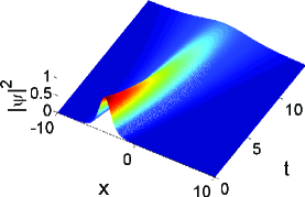
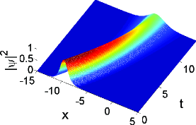
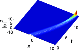
(a) (b) (c)

Figure 1: (Color online) Plot of the solution (13) for (a) $\beta(t)=\sqrt{-\frac{\alpha}{4c}}$, (b) $\beta(t)=\sqrt{-\frac{\alpha}{4c}}\,\tanh(2\sqrt{-c\alpha}\,t)$, and (c) $\beta(t)=-\sqrt{\frac{\alpha}{4c}}\,\tan(2\sqrt{c\alpha}\,t)$. The parameters are $\alpha=\pm 0.005$, $p_{0}=1.0$, $\nu_{0}=1.0$, $a=0$, $c=0.5$, $c_{2}=1$, $c_{4}=\nu_{0}$, $k_{1}=1.0$, $q_{1}=0$, and $\lambda=0.01$. Then the cut-off time is approximately $t_{1}=15.7$. All quantities are dimensionless.

III.2 The dark solitons

Another case that may be of interest in obtaining soliton solutions is when $c_{3}\neq 0$. We may have $f(t)\neq 0$, and reduce the set of equations (8) to

$$\begin{split}&h^{\prime}+2c\beta h=0,\>p^{\prime}+4c\beta p=0,\>q^{\prime}+2ckp=0,\\ &k^{\prime}+4c\beta k+\lambda=0,\>\beta^{\prime}+4c\beta^{2}+\alpha=0,\\ &2cp^{2}c_{4}-\nu h^{2}=0,\>cp^{2}c_{3}-2\nu fh=0,\>f^{\prime}+2c\beta f=0,\\ &\Omega^{\prime}+ck^{2}+\frac{1}{2}cp^{2}c_{2}=0,\>cp^{2}c_{2}-2\nu f^{2}=0.\end{split}$$ (15)

From Eq. (15), it may be shown that, when $c_{3}\neq 0$ the parameters in Eq. (6) must fulfill the constraint $c_{3}^{2}=4c_{2}c_{4}$. In the case where $\alpha$ and $\lambda$ are constants, we choose the parameter $\beta(t)$ as in the previous section to easily solve the above set of equations.

(1) When $\beta(t)$ is constant, the solution of Eq. (15) is:

$$\begin{split}&\beta=\sqrt{\frac{-\alpha}{4c}},\,p(t)=p_{0}e^{-4c\beta t},\,h(t)=h_{0}e^{-2c\beta t},\\ &f(t)=f_{0}e^{-2c\beta t},\,\nu(t)=\nu_{0}e^{-4c\beta t},\\ &k(t)=-\frac{\lambda}{4c\beta}+k_{1}e^{-4c\beta t},\\ &q(t)=\left(-\frac{\lambda}{8c\beta^{2}}+\frac{k_{1}}{4\beta}e^{-4c\beta t}\right)p(t)+q_{1},\\ &\Omega(t)=-\frac{\lambda^{2}}{16c\beta^{2}}t+\frac{c_{2}p_{0}^{2}+2k_{1}^{2}}{16\beta}e^{-8c\beta t}-\frac{\lambda k_{1}}{8c\beta^{2}}e^{-4c\beta t}+\Omega_{1}.\end{split}$$ (16)

In this set of equations, $f_{0}=\frac{c_{3}}{4c_{4}}h_{0}$ is the initial value of $f(t)$. The difference between Eq. (16) and the corresponding results in the previous section resides in the expressions for $f(t)$ and $\Omega(t)$ which change, respectively, the amplitude and the phase of the matter wave.

(2) When $\beta(t)=-\sqrt{\frac{\alpha}{4c}}\,\tan(2\sqrt{c\alpha}\,t)$, solving the set of equations (15), we come to the following results

$$\begin{split}p(t)=&p_{0}\ell(t)^{-1},\,h(t)=h_{0}\ell(t)^{-1/2},\,f(t)=f_{0}\ell(t)^{-1/2},\\ k(t)=&-\frac{\lambda}{2\sqrt{c\alpha}}\,\tan(2\sqrt{c\alpha}\,t)+k_{1}\ell(t)^{-1},\\ q(t)=&\left[-k_{1}\sqrt{\frac{c}{\alpha}}\sin(2\sqrt{c\alpha}\,t)+\frac{\lambda}{2\alpha}\right]p(t)+q_{1},\\ \Omega(t)=&\frac{\lambda^{2}}{4\alpha}t-\frac{\lambda^{2}+2c\alpha(c_{2}p_{0}^{2}+2k_{1}^{2})}{8\alpha\sqrt{c\alpha}}\,\tan(2\sqrt{c\alpha}\,t)\\ &+\frac{\lambda k_{1}}{2\alpha}\ell(t)^{-1}+\Omega_{1},\\ \nu(t)=&\nu_{0}\ell(t)^{-1},\,\ell(t)=|\cos(2\sqrt{c\alpha}\,t)|.\end{split}$$ (17)

We can prevent singularities by considering only the times preceding the cut-off time, i.e., we take $t<t_{1}$. However this particular singularity can be avoided by changing the scattering length in a small time interval that contains each singular time $t_{n}$.

(3) When $\beta(t)=\sqrt{-\frac{\alpha}{4c}}\,\tanh(2\sqrt{-c\alpha}\,t)$, solving the set of equations (15), we obtain the following results

$$\begin{split}p(t)=&p_{0}\ell(t)^{-1},\,h(t)=h_{0}\ell(t)^{-1/2},\,f(t)=f_{0}\ell(t)^{-1/2},\\ k(t)=&-\frac{\lambda}{2\sqrt{-c\alpha}}\,\tanh(2\sqrt{-c\alpha}\,t)+k_{1}\ell(t)^{-1},\\ q(t)=&\left(k_{1}\sqrt{-\frac{c}{\alpha}}\,e^{-2\sqrt{-c\alpha}\,t}+\frac{\lambda}{2\alpha}\right)p(t)+q_{1},\\ \Omega(t)=&\frac{\lambda^{2}}{4\alpha}t-\frac{\lambda^{2}+2c\alpha(c_{2}p_{0}^{2}+2k_{1}^{2})}{8\alpha\sqrt{-c\alpha}}\,\tanh(2\sqrt{-c\alpha}\,t)\\ &+\frac{\lambda k_{1}}{2\alpha}\ell(t)^{-1}+\Omega_{1},\\ \nu(t)=&\nu_{0}\ell(t)^{-1},\,\ell(t)=\cosh(2\sqrt{-c\alpha}\,t).\end{split}$$ (18)

Considering the above results, the general solution of equation (4) for $c_{3}\neq 0$ is given by

$$\psi(z,t)=h(t)\left[\frac{c_{3}}{4c_{4}}+u(\zeta)\right]\,e^{\mathrm{i}(\beta z^{2}+kz+\Omega)},$$ (19)

where $u(\zeta)$ is the solution of Eq. (5) given in Eq. (6). The condition $c_{3}^{2}=4c_{2}c_{4}$ implicitly assumes $c_{4}>0$ since $c_{2}$ is positive. In this case, we easily come to

$$u(\zeta)=\frac{4c_{2}}{-2c_{3}+\>\exp[-\delta\sqrt{c_{2}}\,(\zeta-a)]}.$$ (20)

Eq. (20) is an interesting solution without singularity only when the nonzero coefficient $c_{3}$ is negative. This solution, with Eq. (19), corresponds to a darklike soliton. We portray this solution in Fig. 2. We mention that since $c_{4}>0$, the parameter $\nu_{0}$ is positive and consequently this dark soliton is meant for media that present repulsive interparticle interactions.

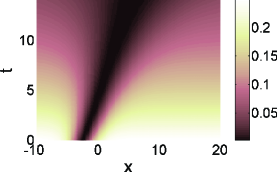
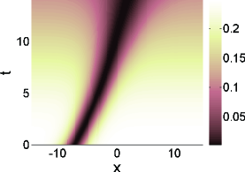
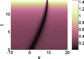
(a) (b) (c)

Figure 2: (Color online) Plot of the solution (19) for (a) $\beta(t)=\sqrt{-\frac{\alpha}{4c}}$, (b) $\beta(t)=\sqrt{-\frac{\alpha}{4c}}\,\tanh(2\sqrt{-c\alpha}\,t)$, and (c) $\beta(t)=-\sqrt{\frac{\alpha}{4c}}\,\tan(2\sqrt{c\alpha}\,t)$. The parameters are $\alpha=\pm 0.005$, $p_{0}=1.0$, $\nu_{0}=-1.0$, $a=0$, $c=0.5$, $c_{2}=1$, $c_{4}=\nu_{0}$, $k_{1}=1.0$, $q_{1}=0$, $\lambda=0.01$, and $\delta=1$. The cut-off time is roughly $t_{1}=15.7$. All quantities are dimensionless.

IV The dynamical properties of the solutions

In order to investigate the dynamical properties of the solutions, we reconsider the above three cases, namely the cases where $\beta(t)=\sqrt{-\frac{\alpha}{4c}}$, $\beta(t)=-\sqrt{\frac{\alpha}{4c}}\,\tan(2\sqrt{c\alpha}\,t)$, and $\beta(t)=\sqrt{-\frac{\alpha}{4c}}\,\tanh(2\sqrt{-c\alpha}\,t)$ which correspond to the respective scattering lengths $\upsilon(t)=\upsilon_{0}\exp(-2\sqrt{-c\alpha}\,t)$, $\upsilon(t)=\upsilon_{0}/|\cos(2\sqrt{c\alpha}\,t)|$, and $\upsilon(t)=\upsilon_{0}/\cosh(2\sqrt{-c\alpha}\,t)$. The solution of equation (4) in each of these cases, for $c_{3}=0$ and $c_{3}\neq 0$, respectively, may read

$$\psi(z,t)=A_{0}s(t)\,\mathrm{sech}[\sqrt{c_{2}}(\zeta-\zeta_{0})]\,e^{\mathrm{i}(\beta z^{2}+kz+\Omega)},$$ (21)

$$\psi(z,t)=A_{0}s(t)\tanh[\frac{1}{2}\sqrt{c_{2}}(\zeta-\zeta_{1})]e^{\mathrm{i}(\beta z^{2}+kz+\Omega)}.$$ (22)

The time-dependent amplitude coefficient, $s(t)=\ell(t)^{-1/2}$, depends on the typical forms of $\beta(t)$ into consideration. We have $A_{0}=\sqrt{\frac{2cc_{2}}{|\nu_{0}|}p_{0}^{2}}$ and $\zeta_{1}=\zeta_{0}-\frac{\ln 2}{\sqrt{c_{2}}}$. Additionally, we recall that $\zeta=p\,z+q$ and $\zeta_{0}=a-\frac{1}{2\sqrt{c_{2}}}\ln(4c_{2}|c_{4}|)$. Without loss of generality, we set $q_{1}=0$.

IV.1 The vanishing matter waves

When $\beta=\sqrt{-\frac{\alpha}{4c}}$, the solution of equation (4) is given in Eqs. (21) and (22), where $\ell$, $p$, $q$, $\beta$, $k$ and $\Omega$ are time-dependent functions given in Eq. (10) for the solution in Eq. (21), and in Eq. (16) for the solution in Eq. (22). As already said, these solutions represent bright and dark solitons, respectively. However they have common dynamical behavior. The width of each of them is proportional to $(p_{0}^{2}c_{2})^{-1/2}\,e^{4c\beta t}$, while the height is proportional to $A=A_{0}\,e^{-2c\beta t}$. In this case, the matter waves have broadening and vanishing properties. As a matter of fact, with time, the height of the matter wave decreases while its width increases. However the number of atoms in the condensate, i.e. $N=\int|\psi|^{2}\mathrm{d}z=-\frac{4c\sqrt{p_{0}^{2}c_{2}}}{\nu_{0}}$, remains unchanged during the propagation of the wave. A plot of this dynamical behavior is given in Figs. 1(a) and 2(a) through the space-time evolution of the square magnitude of the wave function.

The kinematics of the wave can be obtained from $\zeta(z,t)=0$. Hence the motion of the center of mass, taken as the position that corresponds to the peak, is determined by the following equation:

$$z=-\frac{1}{2}k_{1}\sqrt{-\frac{c}{\alpha}}\,e^{-2\sqrt{-c\alpha}\,t}-\frac{\lambda}{2\alpha},$$ (23)

for both dark and bright solitons. At longer times, the center of mass of the wave is driven towards the point $z=-\frac{\lambda}{2\alpha}\equiv z_{\infty}$ which corresponds to the effective trap center. In fact, when the gravitational field is considered, the minimum of the potential is no more on the magnetic trap axis $z=0$, it moves to $z_{\infty}$. Hence the gravitational field drives the wave from the center of the magnetic trap to a region around $z_{\infty}$, where the wave should be confined.

The velocity of the wave packet is $\dot{z}=ck_{1}\,e^{-2\sqrt{-c\alpha}\,t}$. Hence $k_{1}$ appears to be a measurement of the initial velocity of the wave. The velocity exponentially decreases with time. So the choice of the parameters $\lambda$ and $k_{1}$ can seriously affect the dynamics of the matter waves, denouncing the role of the gravitational field in our analysis. The wave packet behaves like a static classical particle for $k_{1}=0$ and like a moving one for $k_{1}\neq 0$. A similar result was obtained in li1 within a special case where the gravitational field is absent ($\lambda=0$) and $c_{3}=0$. The acceleration of the wave packet is $\ddot{z}=-2\sqrt{-c^{3}\alpha}k_{1}\,e^{-2\sqrt{-c\alpha}\,t}$. The acceleration exponentially decreases with time.

When $\beta=\sqrt{-\frac{\alpha}{4c}}\,\tanh(2\sqrt{-c\alpha}\,t)$, the solution of equation (4) is given in Eqs. (21) and (22), where $\ell$, $p$, $q$, $\beta$, $k$ and $\Omega$ are time-dependent functions given in equation (12) for the solution in Eq. (21), and in equation (18) for the solution in Eq. (22). These solutions also represent growing matter waves. The height of each of these waves is proportional to $\left(\frac{2cp_{0}^{2}c_{4}}{\nu_{0}\cosh(2\sqrt{c\alpha}\,t)}\right)^{1/2}$, and the width is proportional to $\frac{1}{p_{0}}\cosh(2\sqrt{c\alpha}\,t)$. The width of the soliton shortens exponentially with time while its height exponentially grows. A display of this dynamical behavior can be found in Figs. 1(b) and 2(b) where we plot the space-time evolution of the wave in the system. The motion of the center of mass of the matter wave is defined by the equation:

$$z=-k_{1}\sqrt{-\frac{c}{\alpha}}\,e^{-2\sqrt{-c\alpha}\,t}-\frac{\lambda}{2\alpha}.$$ (24)

At longer times, the center of mass of the wave is driven towards the point $z=\frac{\lambda}{2\alpha}\equiv z_{\infty}$ which corresponds to the effective trap center. The velocity of the wave packet is $\dot{z}=2ck_{1}\,e^{-2\sqrt{-c\alpha}\,t}$, which is twice the velocity in the previous case. We have observed that the solutions in the cases $\beta(t)=\sqrt{-\frac{\alpha}{4c}}$ and $\beta(t)=\sqrt{-\frac{\alpha}{4c}}\,\tanh(2\sqrt{-c\alpha}\,t)$, both corresponding to an expulsive trapping potential, present similar asymptotic behavior in time. In fact, when $t\rightarrow\infty$ the width, height, and trajectory in both cases become identical.

IV.2 The growing matter waves

When $\beta=-\sqrt{\frac{\alpha}{4c}}\,\tan(2\sqrt{c\alpha}\,t)$, the solution of equation (4) is given in Eqs. (21) and (22), where $\ell$, $p$, $q$, $\beta$, $k$ and $\Omega$ are time-dependent functions given in equation (11) for the solution in Eq. (21), and in equation (17) for the solution in Eq. (22). The corresponding solutions represent growing matter waves. The height of each of these matter waves is proportional to $\left(\frac{2cp_{0}^{2}c_{4}}{\nu_{0}|\cos(2\sqrt{c\alpha}\,t)|}\right)^{1/2}$, and the width is proportional to $\frac{1}{p_{0}}|\cos(2\sqrt{c\alpha}\,t)|$. In the safe time interval, the matter wave becomes thinner and higher. We portray in Figs. 1(c) and 2(c) this dynamical behavior. Close to the cut-off time which is $t_{1}=15.7$, the exponential increase in the amplitude of the wave is so strong that a ”collapse” of the wave may occur. However, by changing the expression of the parameter $\beta(t)$ (which amounts to changing the expression of the s-wave scattering length) in a small time interval that contains each singular time $t_{n}=\frac{(2n+1)\pi}{4\sqrt{c\alpha}}$, the propagation of the matter wave can be kept. It can be changed to $\beta(t)=\sqrt{-\frac{\alpha}{4c}}$ or $\beta(t)=\sqrt{-\frac{\alpha}{4c}}\,\tanh(2\sqrt{-c\alpha}\,t)$. In this case, the width and the height of the wave oscillate in time. Figures 3(a) and 3(b) show the long-time propagation of the matter waves in this case.

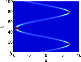
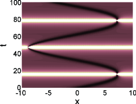
(a) (b)

Figure 3: (Color online) Plot of the long-time evolution of the matter waves in the case where $\beta(t)=-\sqrt{\frac{\alpha}{4c}}\,\tan(2\sqrt{c\alpha}\,t)$ for (a) the solution in Eq. (13), and (b) the solution in Eq. (19). We use $\beta(t)=\sqrt{-\frac{\alpha}{4c}}\,\tanh(2\sqrt{-c\alpha}\,t)$ in small time intervals that contain each singular time $t_{n}=\frac{(2n+1)\pi}{4\sqrt{c\alpha}}$, with $n$ being any integer. The parameters are $\alpha=\pm 0.005$, $p_{0}=1.0$, $\nu_{0}=-1.0$, $a=0$, $c=0.5$, $c_{2}=1$, $c_{4}=\nu_{0}$, $k_{1}=0.8$, $q_{1}=0$, $\lambda=0.01$, and $\delta=1$. All quantities are dimensionless.

The motion of the center of mass of the matter wave is defined by the equation:

$$z=k_{1}\sqrt{\frac{c}{\alpha}}\sin(2\sqrt{c\alpha}\,t)-\frac{\lambda}{2\alpha}.$$ (25)

The velocity of the wave packet is $\dot{z}=2ck_{1}\cos(2\sqrt{c\alpha}\,t)$ while its acceleration is $\ddot{z}=4\sqrt{c^{3}\alpha}k_{1}\cos(2\sqrt{c\alpha}\,t)$. This means that the wave oscillates in time with frequency $f=\frac{\sqrt{c\alpha}}{\pi}$ also equivalent to $(t_{n+1}-t_{n-1})^{-1}$. These oscillations are performed around the position $z=-\frac{\lambda}{2\alpha}$, which corresponds to the effective trap center set by the gravitational field.

In comparison with the results obtained in wamba8 , we see that the role of gravity would not be the same, even qualitatively, for different traps of the BEC system. In fact, the bias magnetic field may be the analog of gravitational field since both fields are represented by the linear term in the trapping potential. From the results of wamba8 , we infer that the kink solitons created in a bias magnetic field alone behave like a classical particle in a pure free fall motion led by the ”gravity” in the $(z,t)$ space. In the present case, the gravitational field is not alone. The presence of the parabolic magnetic potential changes the effect of the gravitational field. For instance, when the initial speed of the bright or dark soliton is zero, then both the velocity and the acceleration at any time are zero too.

The present study suggests three ways to generate bright and dark solitons in BEC systems by time-varying the s-wave scattering length (through the Feshbach resonance) without changing the magnetic potential. This can be done by tuning the scattering length to $g_{0}/|\cos(2\sqrt{c\alpha}\,t)|$ when the condensate is confined in an attractive magnetic trap, i.e. $\alpha$ is positive. We may also tune the scattering length to $g_{0}/\cosh(2\sqrt{-c\alpha}\,t)$, or $g_{0}\exp(-2\sqrt{-c\alpha}\,t)$, in the case of expulsive magnetic trap, i.e. $\alpha$ is negative.

V Conclusion

In conclusion, we have considered the GP equation with time-dependent cubic nonlinearity which describes the dynamics of the BEC matter-waves in a magnetic field and under the effect of a homogeneous gravitational field. With the help of the extended tanh-function method, we have obtained a solution which has as special cases the bright and dark solitons. As has been discussed, these solitons can be generated by properly tuning the s-wave scattering length of the condensed particles, depending on whether the magnetic trapping is attractive or expulsive. The dynamics and kinematics of these matter waves have been presented and discussed.

We have found that the gravity reshapes the repel force of the magnetic trap, and then drives the matter waves towards the region around the position $z=-\frac{\lambda}{2\alpha}$. The matter waves may remain in that position for scattering lengths $g_{0}/\cosh(2\sqrt{-c\alpha}\,t)$ or $g_{0}\exp(-2\sqrt{-c\alpha}\,t)$, and may oscillate around it for $g_{0}/|\cos(2\sqrt{c\alpha}\,t)|$. By comparing the results obtained here with those of wamba8 , we have found that the role of gravitational field depends on the type of trap in which the condensate is confined.

The study of the dynamics and stability of a BEC under the effect of very strong gravitational field, that could occur (in a speculative way) for instance close to black holes, appears to pose an interesting issue to investigate in future works.

References

- (1) V. E. Zakharov and S. V. Nazarenko, Physica D 201, 203 (2005).
- (2) A. Griffin, D. W. Snoke, and S. Stringari, Bose-Einstein Condensation (Cambridge University Press, Cambridge, U. K., 1995).
- (3) A. Mohamadou, E. Wamba, D. Lissouck, and T. C. Kofané, Phys. Rev. E 85, 046605 (2012).
- (4) E. Wamba, T. C. Kofané, and A. Mohamadou, Chin. Phys. B 21, 070504 (2012).
- (5) L.-C. Zhao, Z.-Y. Yang, T. Zhang, and K.-J. Shi, Chin. Phys. Lett. 26, 120301 (2009).
- (6) Z. Yan, K. W. Chow, and B. A. Malomed, Chaos, Solitons and Fractals 42, 3013 (2009); U. Al Khawaja, J. Math. Phys. 51, 053506 (2010).
- (7) R. Murali and K. Porsezian, Physica D 239, 1 (2010).
- (8) Y. Kawaguchi, M. Nakahara, and T. Ohmi, Phys. Rev. A 70, 043605 (2004).
- (9) A. Mohamadou, E. Wamba, S. Y. Doka, T. B. Ekogo, and T. C. Kofané, Phys. Rev. A 84, 023602 (2011).
- (10) J. I. Rivas and A. Camacho, Mod. Phys. Lett. A 26, 481 (2011).
- (11) G. Bertone, D. Hooper, and J. Silk, Physics Reports 405, 279 (2005).
- (12) H. Velten and E. Wamba, Phys. Lett. B, 709 1 (2012); S. J. Si, Phys. Rev. D 50, 3650 (1994); C. G. Böhmer and T. Harko, JCAP 0706, 025 (2007).
- (13) A. Trombettoni and A. Smerzi, Phys. Rev. Lett. 86, 2353 (2001).
- (14) F. Dalfovo, S. Giorgini, L.P. Pitaevskii, and S. Stringari, Rev. Mod. Phys. 71, 463 (1999).
- (15) F. Kh. Abdullaev, B. B. Baizakov, S. A. Darmanyan, V. V. Konotop, and M. Salerno, Phys. Rev. A 64, 043606 (2001).
- (16) P. S. Julienne, F. H. Mies, E. Tiesinga, and C. J. Williams, Phys. Rev. Lett. 70, 1880 (1997).
- (17) A. Camacho, L. F. Barragán-Gil, and A. Macías, Cent. Eur. J. Phys. 8, 717 (2010).
- (18) A. J. Legget, Rev. Mod. Phys. 73, 307 (2001).
- (19) J. R. Ensher, PhD thesis, University of Colorado (Boulder, USA, 1998).
- (20) I. K. Kulikov, arXiv:cond-mat/0205330v3 [cond-mat.stat-mech] (2002); I. K. Kulikov, Int. J. Theor. Phys. 41, 1481 (2002).
- (21) B. P. Anderson and M. A. Kasevich, Science 282, 1686 (1998); W. Zhang and D. F. Walls, Phys. Rev. A 57, 1248 (1998).
- (22) A.-X. Zhang and J.-K. Kue, Phys. Rev. A 75, 013624 (2007); F. Kh. Abdullaev, R. M. Galimzyanov, and Kh. N. Ismatullaev, J. Phys. B: At. Mol. Opt. Phys. 41, 015301 (2008).
- (23) Ph. Courteille, R. S. Freeland, D. J. Heinzen, F. A. van Abeelen, and B. J. Verhaar, Phys. Rev. Lett. 81, 69 (1998); E. Timmermans, P. Tommasini, M. Hussein, and A. Kerman, Physics Reports 315, 199 (1999).
- (24) G. Nandi, R. Walser, E. Kajari, and W. P. Schleich, Phys. Rev. A 76, 063617 (2007).
- (25) H.-M. Li, Chin. Phys. 15, 2216 (2006).