Edinburgh 2012/13 IPPP/12/45, DCPT/12/90 CP3-Origins-2012-017, DIAS-2012-18 W Plus Multiple Jets at the LHC with High Energy Jets

Abstract

We study the production of a $W$ boson in association with $n$ hard QCD jets (for $n\geq 2$), with a particular emphasis on results relevant for the Large Hadron Collider (7 TeV and 8 TeV). We present predictions for this process from High Energy Jets, a framework for all-order resummation of the dominant contributions from wide-angle QCD emissions. We first compare predictions against recent ATLAS data and then shift focus to observables and regions of phase space where effects beyond NLO are expected to be large.

1 Introduction

There is already a wealth of analyses of data from the Large Hadron Collider (LHC), many of which are beginning to stress-test the perturbative descriptions of proton-proton collisions at LHC energies. It is of course essential to demonstrate to what level the Standard Model (SM) processes are understood. This is often the first step towards a discovery (or limit) on new physics.

A particularly interesting process is $W$ plus jets where, in the leptonic decay mode, the neutrino leads to events with missing transverse energy. The combination of multiple jets and missing energy is a very common signal in models beyond the Standard Model, arising from a production mechanism with QCD charged particles followed by decay chains ending with a (semi-)stable, weakly interacting particle.

There have been a number of data analyses of this channel already by both the ATLAS [1, 2] and CMS [3] experiments. The production of a $W$ boson in association with jets is also a clean environment for QCD studies, and as such could be an important testing ground for experimental methods used to study methods like e.g. jet vetos. What is learned in $W$ plus jets could be applied in searches for the Higgs boson and other new physics.

There has also been a great deal of recent theoretical progress in fixed-order calculations of this channel, where the state-of-the-art is now $W$ plus four jets in the leading colour approximation [4], or $W$ plus three jets in the full colour dressing  [5, 6, 7]. The NLO calculations lead to very good agreement for total cross sections and, for the right scale choices, also for several differential distributions.

Much work has been reported on estimating effects beyond NLO. The NLO calculations for $W$-production in association with up to two [8] and three jets [9] have been systematically merged with a parton shower. Furthermore, LoopSim [10] has also been applied to approximate higher fixed-order contributions to $W$ production in regions where the $K$-factor is large.

In this study we present the application of the High Energy Jets (HEJ) formalism developed in Refs. [11, 12] to the process of $W$-production (and leptonic decay) in association with at least two hard jets. The general formalism has previously been applied to pure multi-jet production [13], with the results from the accompanying flexible Monte Carlo implementation used in several analyses of LHC data[14, 15, 16]. The all-order results of HEJ are complementary to those obtained from a parton shower approach. The simplifications made by HEJ to the perturbative series to allow all-order results to be obtained become exact in the limit of large invariant mass between all particles. This corresponds to the limit where also the (B)FKL amplitudes[17, 18, 19] are exact. The production of $W$+dijets was previously studied within the BFKL formalism[20]. Compared to this, the present formalism introduces several major improvements: it relaxes several kinematic assumptions made in the earlier study, improves the accuracy of the resummation, and introduces matching to fixed order results.

In pure HEJ, there are no collinear singularities, no shower and no hadronisation: the output is a pure partonic calculation. However, this can all be consistently included by merging the results with a shower Monte Carlo by a procedure which avoids double-counting[21]. Such double-counting would otherwise arise in particular in the soft regions, which are treated in both HEJ and a parton shower.

This paper is structured as follows. In Section 2 we study the various production channels for $W$ plus jets at the LHC and properties of the jet radiation. In Section 3 we summarise the construction of the HEJ amplitudes and their implementation in a fully flexible Monte Carlo. The resulting program is available at http://cern.ch/hej. In Section 4 we compare predictions for kinematic distributions to LHC data, before embarking in Section 5 on a discussion of regions of phase space and observables where effects beyond NLO are expected to be large. We end in Section 6 with a brief discussion.

2 The Anatomy of $W$ Plus Jets at the LHC

In this section, we focus on the production of a $W^{+/-}$-boson (followed by a leptonic decay) in association with at least two jets. We will from now denote both $W^{+}$ and $W^{-}$ as $W$, and both electron and positron as $e$. Furthermore, we will apply the following acceptance cuts:

$$\begin{split}p_{\perp j}>30\ {\rm GeV},\quad&\left|\eta_{j}\right|<4.4,\quad p_{\perp e}>20\ {\rm GeV},\quad\left|\eta_{e}\right|<2.5,\quad\cancel{E}_{T}>25\ {\rm GeV},\\ M_{\perp W}&=\sqrt{2\ p_{\perp e}\ p_{\perp\nu}\ (1-\cos(\phi_{e}-\phi_{\nu}))}\ >40\ {\rm GeV},\end{split}$$ (1)

where $\eta$ is the pseudorapidity and $\phi$ is the azimuthal angle of the respective particle momentum.

The kinematic requirements of the two jets and the charged lepton alone ensure that the parton density functions are probed only for a light-cone momentum fraction $x$ larger than $3.4\cdot 10^{-4}$ at 7 TeV ($1.7\cdot 10^{-4}$ at 14 TeV). The neutrino momentum will contribute further to the momentum fraction, and thus the dynamics is well within the regime where standard, collinearly factorised pdfs and hard scattering matrix elements describe the cross sections accurately. We will therefore concentrate on perturbative higher order corrections within this framework, and not discuss small-$x$ issues like $k_{\perp}$-factorisation or unintegrated pdfs. We will use the standard MSTW2008NLO[22] pdf set throughout. The accompanying program is interfaced to LHAPDF, so any publicly available pdf set can be used.

In earlier studies[23, 13, 21] we established a strong connection between the average number of hard jets in events, and the rapidity difference between the most forward/backward hard jet in pure jet production. This is a result not just of the opening of phase space for the emission of additional jets, but also the possibility of a colour octet exchange between particles ordered in rapidity. Such a correlation was recently confirmed by data[14].

It is obviously relevant to discuss the extent to which the behaviour observed in pure jets is relevant for the production of $W$+dijets. The explanation from BFKL[17, 18, 19, 24] for the correlation between the average number of jets and the rapidity span of the events[23] relies on the higher order corrections to the dijet processes which allow for a colour octet exchange between all rapidity-ordered partons.

Subprocess	$\sigma_{2j}\ [pb]$
$qq^{\prime}\to Wqq^{\prime}$	11.6
$qg\to Wqg$	67.7
$q\bar{q}\to Wq\bar{q}$	9.9
$q\bar{q}\to Wgg,Wq^{\prime}\bar{q}^{\prime}$	5.8
$gg\to Wq\bar{q}$	4.3

Table 1: Leading order cross sections (in pb) for the production of a $W$ boson in association with two jets for the LHC at $\sqrt{s}=7$ TeV. The subprocesses above the horizontal line are those which allow a colour octet exchange between the two initial state (and the two final state) partons, while those below do not.

In Table 1 we have listed the sub-process contributions to the cross section for $Wjj$-production at leading order within the cuts of Eq. (1). The processes above the horizontal line are those which allow colour octet exchange between the two initial (and the two final state) partons. Clearly, these dominate the cross section. Such colour exchanges will dominate the higher order corrections in the limit of large rapidity separation between all partons. However, this requirement also means that quarks are produced only as the partons which are extremal in rapidity in the scattering. One could worry that the cut on the centrality of the charged lepton from the $W$ decay would force the quark-line emitting the $W$ to also be central, thereby suppressing the phase space for a large rapidity span between the jets. In figure 1 we plot $1/\sigma\mathrm{d}\sigma/\mathrm{d}(y_{f}-y_{b})$ for $W+$dijets at leading order.

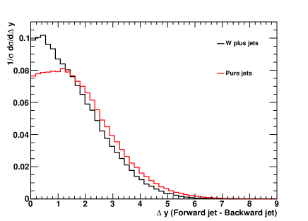
Figure 1: The normalised distribution of the rapidity difference between the two jets, $\mathrm{d}\sigma/\mathrm{d}(y_{f}-y_{b})$, for $W$ plus two jets at tree-level (black), within the cuts of Eq. (1). Also shown for comparison is the same distribution for dijet production, with equivalent cuts on the jets.

Also shown for comparison is the equivalent distribution for pure dijets. While the $W+$dijets distribution is slightly more peaked at zero, there is very little difference in the shape of the distributions above a rapidity span of around 1.5, indicating that a systematic resummation of radiation between jets is just as relevant for $W$+dijets as for dijets.

The analyses presented above demonstrate that at the LHC, the sub-processes allowing for colour octet exchange in the $t$-channel dominate the rate for $W$+dijets. This observation will be the guiding principle for the resummation for $W$+jets implemented in HEJ.

3 $W$ Plus Jets in High Energy Jets

The framework of High Energy Jets (HEJ)[11, 12] constructs explicit approximations to the real and virtual corrections to the perturbative hard scattering matrix element at any order. Furthermore, matching to the full tree-level results for the first few higher order corrections are implemented through a jet merging algorithm. The framework, and the application to the description of $W$+jets is described in this section.

3.1 All-Order Amplitudes

The starting point for the HEJ approach is an approximation to the hard-scattering matrix element for $2\to n$ partons plus the leptonic decay products of the $W$. This is built from the dominant terms in the High Energy (or Multi-Regge Kinematic) limit, which is defined as:

$$\begin{split}&\forall i,j\quad s_{ij}\to\infty\quad|p_{i\perp}|\sim|p_{j\perp}|\\ {\rm or}\ {\rm equivalently}\quad&i\in\{1,n-1\}\quad y_{i-1}\ll y_{i}\ll y_{i+1}\quad|p_{i\perp}|\sim|p_{j\perp}|,\end{split}$$ (2)

where $i,j$ label the $n$ final state quarks and gluons, ordered in rapidity. There is no constraint on the momenta of the $e,\nu$.

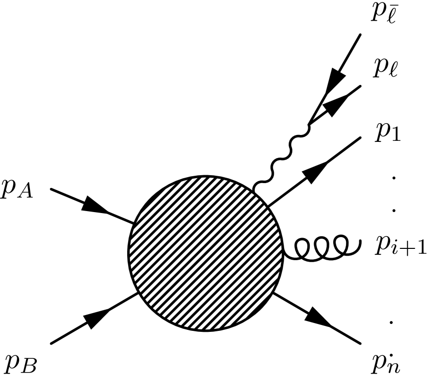
$\longrightarrow$

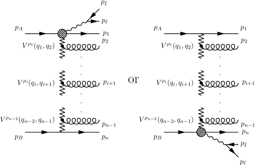
Figure 2: Sample kinematics for $qQ\to q^{\prime}g\ldots gQ$. The diagrams on the right-hand side show the dominant kinematic configurations in the High Energy limit where the outgoing partons are drawn and numbered in order of increasing rapidity. The effective vertices, $V(q_{i},q_{i+1})$, are defined in Eq. (10).

In this limit, the scattering amplitude is dominated by the poles in the $t$-channel momenta, as depicted in Fig. 2 and defined as

$$q_{i}=p_{A}-(p_{e}-p_{\nu})\cdot\delta-p_{1}-\ldots-p_{i-1},$$ (3)

where $\delta=1$ if the $W$ is interpreted as emitted from the quark line with momenta $p_{A},p_{1}$, and $\delta=0$ otherwise. The numbering of momenta is according to decreasing rapidity, $A$ indicates the forward moving incoming parton, $B$ the backward moving one. The leading contributions to the poles arise from the particle and momentum configurations which allow for a colour octet exchange between each neighbouring (in rapidity) pair of partons. We will call these FKL configurations. For example, in dijet production $ug\to ug$ and $ud\to uggd$ are FKL configurations with that rapidity order, while $ug\to gu$ and $ud\to us\bar{s}d$ are not. Each relaxation of a colour ordering induces a relative suppression of $1/s$ in the squared matrix element and hence is subdominant in the High Energy limit. The all-order treatment in HEJ currently only describes FKL configurations. Other contributions are included order by order with standard tree-level matrix elements.

Scattering amplitudes factorise according to rapidity in the High Energy limit. Based on the work of Ref.[11, 12, 13] we choose a form of amplitudes for each helicity configuration, which is a) gauge invariant, b) exact in the MRK limit, and c) sufficiently fast to evaluate that a numerical integration over the phase space of the sum over any number of emissions can be accurately evaluated. For the case at hand, the tree-level approximation to the square of the matrix element is

$$\begin{split}\overline{\left|\mathcal{M}_{\rm HEJ}^{t}(\{p_{i},p_{e},p_{\nu}\})\right|}^{2}=\ &\frac{1}{4\ (N_{\!C}^{2}-1)}\ \left\|S_{f_{a}f_{b}\to f_{1}f_{n}\ p_{e}\ p_{\nu}}\right\|^{2}\\ &\cdot\ \left(g^{2}\ K_{f_{1}}\ \frac{1}{t_{1}}\right)\cdot\ \left(g^{2}\ K_{f_{n}}\ \frac{1}{t_{n-1}}\right)\\ &\cdot\prod_{i=1}^{n-2}\left({g^{2}C_{A}}\ \left(\frac{-1}{t_{i}t_{i+1}}V^{\mu}(q_{i},q_{i+1})V_{\mu}(q_{i},q_{i+1})\right)\right)\\ \end{split}$$ (4)

The bold-face $\mathbf{p}_{i}$ indicates the transverse components, with $\mathbf{p}_{i}^{2}>0$. Each part of this equation will now be explained in full detail. $\left\|S_{f_{a}f_{b}\to f_{1}f_{n}\ p_{e}\ p_{\nu}}\right\|^{2}$ is the helicity sum of the contracted currents

$$||S_{ud\to d\nu_{\ell}\bar{\ell}d}||^{2} =\frac{g_{W}^{4}}{4}\left|\frac{1}{p_{W}^{2}-M_{W}^{2}+i\ \Gamma_{W}M_{W}}\right|^{2}\sum_{h_{b},h_{2}}|S_{ud\to d\nu_{\ell}\bar{\ell}d}^{-h_{b}\to-h_{2}--}|^{2},$$ (5)

where we have picked the case of the extremal partons to represent the scattering $ud\to d\nu_{\ell}\bar{\ell}d$ as an example, and the incoming $u$-quark as the forward-moving parton (i.e. with momentum $p_{a}$). The spinor contraction for each helicity is simply

$$S^{-h_{b}\to-h_{2}--}_{ud\to dd\nu_{\ell}\bar{\ell}}=j_{W\mu}(i,\ell,\bar{\ell},o)\ g^{\mu\nu}\ \bar{u}^{h_{2}}(p_{2})\gamma_{\nu}u^{h_{b}}(p_{b})$$ (6)

with

$$j_{W}^{\mu}(i,\ell,\bar{\ell},o)=\bar{u}^{-}(p_{\rm out})\left(\gamma^{\alpha}\frac{\cancel{p}_{W}+\cancel{p}_{\rm out}}{(p_{W}+p_{\rm out})^{2}}\ \gamma^{\mu}+\gamma^{\mu}\frac{\cancel{p}_{\rm in}-\cancel{p}_{W}}{(p_{\rm in}-p_{W})^{2}}\ \gamma^{\alpha}\right)u^{-}(p_{\rm in})\ \cdot\ \bar{u}^{-}(p_{\ell})\gamma_{\alpha}u^{-}(p_{\bar{\ell}}).$$

(7)

This is simply the spinor representation of a fermion line emitting a (decaying) W and a (possibly off-shell) gluon, as represented by the figure in the equation above.

In $qg$-initiated processes, the $W$ is obviously attached to the quark line. However, for $qQ$-initiated processes, the $W$ emission can be assigned to one or both lines. However, the formalism developed needs the $W$-emission to be assigned to just one line. Therefore, we assign the $W$ to either quark line $a$ or $b$ on an event-by-event basis according to the ratio:

$$a:b\quad=\qquad e^{-|y_{a}-y_{W}|}:e^{-|y_{b}-y_{W}|},$$ (8)

so that the quark closest in rapidity to the $W$ is favoured, but not chosen exclusively. The event weight is adjusted so the outcome is independent of this choice. Picking one specific quark line allows for the definite assignment of $t$-channel momenta in Eq. (3) and the calculation of the squared amplitude in Eq. (5).

For a quark line, the colour factor $K_{f_{i}}$ is just $C_{F}$. We will use the results of Ref.[12] to include the case of $qg\to q^{\prime}g\cdots gg\ell\bar{\ell}$ by simply using a colour factor depending on the light-cone momenta fraction $z=p_{n}^{-}/p_{b}^{-}$ of the scattered gluon:

$$K_{g}=\left[\frac{1}{2}\ \frac{1+z^{2}}{z}\ \left(C_{A}-\frac{1}{C_{A}}\right)+\frac{1}{C_{A}}\right].$$ (9)

It can be seen that $K_{g}\to C_{A}$ for $p_{n}^{-}/p_{b}^{-}\to 1$, in agreement with the well-known result in this limit[25].

The $t$-channel propagator denominators are given by $t_{i}=q_{i}^{2}$, with $q_{i}$ defined in Eq. (3). Additional (gluon) emissions are approximated with a string of effective emission vertices [11], given by:

$$\begin{split}V^{\rho}(q_{i},q_{i+1})=&-(q_{i}+q_{i+1})^{\rho}\\ &+\frac{p_{A}^{\rho}}{2}\left(\frac{q_{i}^{2}}{p_{i+1}\cdot p_{A}}+\frac{p_{i+1}\cdot p_{B}}{p_{A}\cdot p_{B}}+\frac{p_{i+1}\cdot p_{n}}{p_{A}\cdot p_{n}}\right)+p_{A}\rightarrow p_{1}\\ &-\frac{p_{B}^{\rho}}{2}\left(\frac{q_{i+1}^{2}}{p_{i+1}\cdot p_{B}}+\frac{p_{i+1}\cdot p_{A}}{p_{B}\cdot p_{A}}+\frac{p_{i+1}\cdot p_{1}}{p_{B}\cdot p_{1}}\right)-p_{B}\rightarrow p_{n}\end{split}$$ (10)

where $p_{g}=q_{i+1}-q_{i}$ is the momentum of the emitted gluon. This simple structure makes it very fast to integrate in an efficient phase-space generator [26, 27]. This allows the number of final state particles to be treated as a variable in the integration. The four-momenta of all final state particles is available in every event, allowing arbitrary cuts and analyses.

An infrared pole will be generated from the phase space integration over the region $|p_{g,i}|\to 0$ for each $i$. In these regions,

$$\frac{-1}{t_{i}t_{i+1}}V^{\mu}(q_{i},q_{i+1})V_{\mu}(q_{i},q_{i+1})\to\frac{4}{\mathbf{p}_{i}^{2}}.$$ (11)

The simple $4/\mathbf{p}_{i}^{2}$-term is therefore used as a real-emission subtraction term (with the integral form added to the virtual corrections). Infrared poles are also generated by the inclusion of virtual corrections to the $t$-channel gluon propagator factors. These are accounted for by the Lipatov Ansatz[24], which replaces the standard gluon propagator factor $1/t_{i}$ with

$$\frac{1}{t_{i}}\ \to\ \frac{1}{t_{i}}\ \exp\left[\hat{\alpha}(q_{i})(y_{i-1}-y_{i})\right]$$ (12)

with

$$\hat{\alpha}(q_{i}) =-g^{2}\ C_{\!A}\ \frac{\Gamma(1-\varepsilon)}{(4\pi)^{2+\varepsilon}}\frac{2}{\varepsilon}\left({\bf q}^{2}/\mu^{2}\right)^{\varepsilon}.$$ (13)

We organise the cancellation of the poles from these two sources using dimensional regularisation, the subtraction term confined to a small region of real emission phase space with ${\bf p}_{i}^{2}<\lambda^{2}$. Further details in Ref.[13].

The final expression for the all-order regularised square of the scattering matrix element is then given as

$$\begin{split}\overline{\left|\mathcal{M}_{\rm HEJ}^{\mathrm{reg}}(\{p_{i},p_{e},p_{\nu}\})\right|}^{2}=\ &\frac{1}{4\ (N_{\!C}^{2}-1)}\ \left\|S_{f_{a}f_{b}\to f_{1}f_{n}\ p_{e}\ p_{\nu}}\right\|^{2}\\ &\cdot\ \left(g^{2}\ K_{f_{1}}\ \frac{1}{t_{1}}\right)\cdot\ \left(g^{2}\ K_{f_{n}}\ \frac{1}{t_{n-1}}\right)\\ &\cdot\prod_{i=1}^{n-2}\left({g^{2}C_{A}}\ \left(\frac{-1}{t_{i}t_{i+1}}V^{\mu}(q_{i},q_{i+1})V_{\mu}(q_{i},q_{i+1})-\frac{4}{\mathbf{p}_{i}^{2}}\ \theta\left(\mathbf{p}_{i}^{2}<\lambda^{2}\right)\right)\right)\\ &\cdot\prod_{j=1}^{n-1}\exp\left[\omega^{0}(q_{j},\lambda)(y_{j-1}-y_{j})\right],\\ \omega^{0}(q_{j},\lambda)=\ &-\frac{\alpha_{s}N_{C}}{\pi}\log\frac{{\bf q}_{j}^{2}}{\lambda^{2}}.\end{split}$$ (14)

3.2 Merging with Fixed Order

The regularised matrix elements in Eq. (14) allow for an integration over the momenta of all particles. The cross section is then obtained as

$$\begin{split}\sigma_{W+2j}^{\mathrm{resum}}=&\sum_{f_{1},f_{2}}\ \sum_{n=2}^{\infty}\ \prod_{i=1}^{n}\left(\int_{p_{i\perp}=0}^{p_{i\perp}=\infty}\frac{\mathrm{d}^{2}\mathbf{p}_{i\perp}}{(2\pi)^{3}}\ \int\frac{\mathrm{d}y_{i}}{2}\right)\ \int\frac{\mathrm{d}^{3}p_{e}}{(2\pi)^{3}\ 2E_{e}}\ \ \int\frac{\mathrm{d}^{3}p_{\nu}}{(2\pi)^{3}\ 2E_{\nu}}\ \\ &\frac{\overline{|\mathcal{M}_{\mathrm{HEJ}}^{\mathrm{reg}}(\{p_{i},p_{e},p_{\nu}\})|}^{2}}{\hat{s}^{2}}\cdot\ x_{a}f_{A,f_{1}}(x_{a},Q_{a})\ \cdot x_{2}f_{B,f_{2}}(x_{b},Q_{b})\\ &\times(2\pi)^{4}\ \delta^{2}\!\!\left(\sum_{k=1}^{n}\mathbf{p}_{k\perp}+p_{e\perp}+p_{\nu\perp}\right)\ \mathcal{O}_{2j}(\{p_{i}\}),\end{split}$$ (15)

where the first sum is over the flavours $f_{1},f_{2}$ of incoming partons. In order to stay within the relevant kinematics for the formalism, we require the two extremal partons to be part of the extremal hard jets identified by the jet clustering algorithm. Furthermore, we require at least two such hard jets to be present. These requirements are implemented by the jet observable $\mathcal{O}_{2j}$ in Eq. (15). The distribution of any observable can be obtained by simply binning the cross section in Eq. (15) in the appropriate variable formed from the explicit momenta. Obviously, multi-jet rates can also be calculated by multiplying by further multi-jet observables $\mathcal{O}_{3j},\mathcal{O}_{4j},\ldots$.

The simple structure of the HEJ framework makes it feasible to merge with other theoretical descriptions, where relevant. By default, HEJ contains matching to fixed-order tree-level amplitudes in two different ways. Firstly, for flavour and momentum configurations arising in the resummation described above, the approximation to the $n$-jet production can be reweighted to full tree-level accuracy. This is achieved by a merging procedure which clusters all the $m$ momenta generated by the resummation into $n$ on-shell momenta $\left\{p^{\mathrm{new}}_{\mathcal{J}_{l}}(\{p_{i}\})\right\}$ close to the reconstructed jet momenta[13]. The event weight is then adjusted with the ratio of the full $n$-jet matrix element (evaluated by MadGraph [28]) to the approximate one obtained as the $\alpha_{s}^{n}$-expansion of Eq. (14) to the $n$-jet production rate (obtained from Eq. (4)). Currently, reweighting up to $n=4$-jets is applied. The reweighted resummed cross section is then found as

$$\begin{split}\sigma_{W+2j}^{\mathrm{resum,merged}}=&\sum_{f_{1},f_{2}}\ \sum_{n=2}^{\infty}\ \prod_{i=1}^{n}\left(\int_{p_{i\perp}=0}^{p_{i\perp}=\infty}\frac{\mathrm{d}^{2}\mathbf{p}_{i\perp}}{(2\pi)^{3}}\ \int\frac{\mathrm{d}y_{i}}{2}\right)\ \int\frac{\mathrm{d}^{3}p_{e}}{(2\pi)^{3}\ 2E_{e}}\ \ \int\frac{\mathrm{d}^{3}p_{\nu}}{(2\pi)^{3}\ 2E_{\nu}}\ \\ &\frac{\overline{|\mathcal{M}_{\mathrm{HEJ}}^{\mathrm{reg}}(\{p_{i},p_{e},p_{\nu}\})|}^{2}}{\hat{s}^{2}}\cdot\ x_{a}f_{A,f_{1}}(x_{a},Q_{a})\ \cdot x_{2}f_{B,f_{2}}(x_{b},Q_{b})\\ &\times\ \sum_{m=2}^{4}\mathcal{O}_{mj}^{e}(\{p_{i}\})\ w_{m-\mathrm{jet}}\\ &\times(2\pi)^{4}\ \delta^{2}\!\!\left(\sum_{k=1}^{n}\mathbf{p}_{k\perp}+p_{e\perp}+p_{\nu\perp}\right)\ \mathcal{O}_{2j}(\{p_{i}\}),\end{split}$$ (16)

with $\mathcal{O}_{mj}^{e}$ the exclusive $m$-jet observable and

$$w_{n-\mathrm{jet}}\equiv\frac{\overline{\left|\mathcal{M}^{\mathrm{Tree}}\left(\left\{p^{\mathrm{new}}_{\mathcal{J}_{l}}(\{p_{i}\})\right\}\right)\right|}^{2}}{\overline{\left|\mathcal{M}_{\mathrm{HEJ}}^{t}\left(\left\{p^{\mathrm{new}}_{\mathcal{J}_{l}}(\{p_{i}\})\right\}\right)\right|}^{2}}.$$ (17)

The event sample arising from the equation above is finally supplemented with the kinematic configurations (up to $n=4$-jets) not arising in this resummation. This is obviously a very naïve matching, and improvements along a CKKW-L[29, 30] procedure should be pursued. Alternatively, the HEJ resummation could be expanded to cover configurations formally subleading in the MRK limit.

In the meantime, we can assess the importance of the fixed-order contributions with the present implementation. Figure 3 shows the rapidity span distribution including different levels of matching. Clearly at small rapidity spans, the non-FKL 2-jet matching is dominating the cross-section, demonstrating the importance of including these contributions. The impact diminishes as the rapidity span increases (as expected). The further addition of non-FKL 3- and 4-jet matching (blue and black lines) is visible but less significant for this variable.

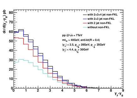
Figure 3: The rapidity span distribution from HEJ for inclusive $W$ plus dijet production for the FKL configurations (turquoise), with 2-jet non-FKL added (red), then with 3-jet non-FKL matching added (blue) and lastly also including 4-jet non-FKL merging.

Another important direction for the development of HEJ is work on merging with parton showers. HEJ is constructed to approximate the emission of QCD particles at wide angles. While this includes emissions with transverse momentum as low as 1 GeV, it does not include a description of collinear emissions. This can be added by consistently merging with a parton shower program. However, this must be done with some care to avoid double-counting soft emissions. A subtraction scheme to merge with the Ariadne parton shower [30] has been developed [21], and further work is ongoing to merge with other parton shower implementations.

The resummation and merging procedures discussed so far do not rely on a particular choice for the factorisation and renormalisation scales. We have implemented four different scale choices for $\mu_{R}=\mu_{F}$ (although they in principle do not need to be set equal) as follows. We list them here with the numbering scheme applied in the input file for the program:

• Fixed scale of your choice, set in “scale”.

• $H_{T}/2$, where $H_{T}$ is the transverse sum of all final state particles including $p_{\perp\ell^{\pm}}$ and $\cancel{E}_{T}=p_{\perp\nu}$.

• $p_{\perp{\rm max}}$ – the maximum $p_{\perp}$ of any single jet in each event.

• The geometric mean of the identified hard jets, $\left(\prod_{j=1}^{n}p_{\perp j}\right)^{1/n}$.

In addition, there is the option to add logarithmic corrections, mimicking the part of the NLL BFKL corrections which are proportional to the LL kernel. These can be included by setting the “logcorrect” parameter in the input file to 1. These corrections modify $\omega_{0}(q,\lambda)$ of Eq. (14) to give instead

$$\begin{split}\omega_{0}(q_{j},\lambda)=&\ -\frac{\alpha_{s}(\mu^{2})\ C_{\!A}}{\pi}\ln\left(\frac{\mathbf{q}_{j}^{2}}{\lambda^{2}}\right)\ \left(1+\frac{\alpha_{s}(\mu^{2})}{2}\frac{\beta_{0}}{4\pi}\ln\frac{\mu^{4}}{\mathbf{q}_{j}^{2}\lambda^{2}}\right),\\ \beta_{0}=&\frac{11}{3}N_{\!C}-\frac{2}{3}n_{\!f}\end{split}$$ (18)

while for the real emission vertices the coupling is multiplied by

$$\left(1-\alpha_{s}(\mu^{2})\frac{\beta_{0}}{4\pi}\ln\mathbf{p}_{i}^{2}/\mu^{2}\right).$$ (19)

See Ref. [13] for a full discussion. For the results presented in the next two sections we have used $\mu_{R}=\mu_{F}=H_{T}/2$ and included the logarithmic corrections associated with the scale. This last choice is motivated by reducing the impact of the NLL corrections. These choices are not an indication of an optimised fit to data, and other scale choices could be studied.

4 Comparison to LHC data

Having outlined the description of $W$ plus jets in HEJ, in this section we compare the resulting predictions to the data we have from the LHC. A recent ATLAS study of $W$ production in association with jets [2] gave results for many interesting distributions, using the full 2010 data sample of 36 pb^-1. The cuts used in that study, and therefore here, match those of section 2 (eq. (1)), with the addition of an isolation cut, $\Delta R(\ell,j)>0.5$, applied to all jets. Throughout, the HEJ predictions are shown together with a band indicating the variation found when varying the renormalisation and factorisation scale by a factor of two in either direction. Obviously, this variation is only a rough indication of the true uncertainty of the prediction, with similar caveats as for a fixed order calculation. The total time required to generate the event sample of this section, and the next, is roughly one day on a single PC.

We begin in figure 4 by showing comparisons for the distributions of $H_{T}$ and the transverse momentum of the hardest jet, in events of 2,3 and 4 jets. The left plot shows the $H_{T}$ distribution for inclusive $W+2,3$ and $4$-jet samples. In all but the bin of lowest $H_{T}$ for the inclusive $Wjj$ production (where the experimental uncertainty is relatively large), the predictions from HEJ overlaps with the data, within the quoted uncertainties. It is clear from this plot that at for $H_{T}$ larger than roughly 400 GeV, the suppression from requiring one additional hard jet is only roughly a factor 2, and not $\alpha_{S}$. HEJ is developed particularly to deal with the case of a large impact from high jet multiplicity. A comparison between HEJ and other theoretical descriptions for this distribution has recently appeared in [31].

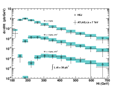
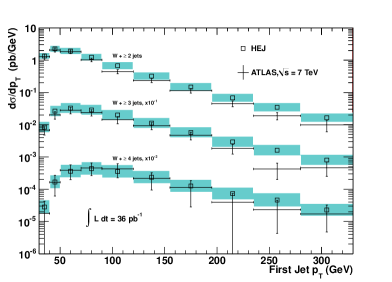
Figure 4: Left: The $W~{}+$ jets cross section as a function of $H_{T}$, the scalar sum of the transverse momenta of the jets, the charged lepton and the missing transverse momentum. Right: The $W~{}+$ jets cross section as a function of the transverse momentum of the hardest jet in the event. The data points, in this and subsequent plots in this section, are taken from Ref. [2].

The right-hand plot of figure 4 shows the transverse momentum distribution of the hardest jet in each event, again for inclusive $W+2,3$ and $4$-jet events. This, more inclusive, variable is less sensitive to the description of additional radiation like that included in HEJ, and still one sees good agreement between the HEJ prediction and data.

Figure 5 shows the distributions for the invariant mass of the hardest 2, 3 and 4-jets in the event. This is more sensitive to the topology of the events, in addition to the overall momentum scale. As the number of jets increases, the peak of this distribution moves away from the kinematic minimum to higher values of invariant mass. Over this wider range of momentum, we again find a very close agreement between the HEJ predictions and the data.

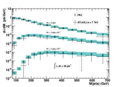
Figure 5: $W~{}+$ jets cross section as a function of the invariant mass of two, three and four jets separately.

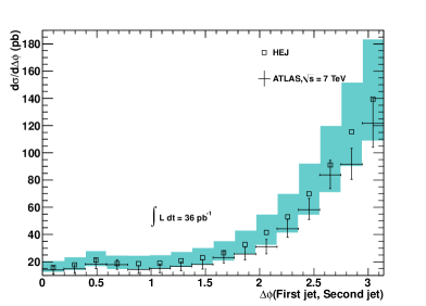
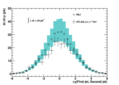
Figure 6: Left: The $W~{}+$ jets cross section shown as a function of the absolute difference in azimuthal angle between the two hardest jets, $|\phi_{jet1}-\phi_{jet2}|$. Right: The $W~{}+$ jets cross section as a function of rapidity difference of the two hardest jets.

The final plots we show in this section, in figure 6, probe the relative position of the two hardest jets in each event. Firstly, the left-hand plot shows the distribution of the difference in azimuthal angle between the two hardest jets. This is peaked at $\Delta\phi=\pi$. For pure dijet production at tree-level, the azimuthal distribution is a delta-functional at $\pi$, and higher order corrections smear out this distribution, which however remains peaked at $\Delta\phi=\pi$. The fact that data for $Wjj$ shows a similar structure for the azimuthal distribution indicates that this process proceeds less like one parton recoiling against a $W$, and then splitting into further jets and more like a dijet scattering with a $W$-emission. This indeed is the mechanism implemented in HEJ, and it describes the data well across the distribution.

The right-hand plot in figure 6 shows the distribution of the difference in rapidity between the two hardest jets. It is clear that the HEJ description is slightly high at the peak around $\Delta y=0$. This is precisely the region where the impact of matching to fixed-order is largest, and the impact of the naïve scheme currently applied will be greatest. This is an important area of future development for HEJ. However, we see that across the analyses, the description of $W+$jets as currently implemented in HEJ describes existing LHC data very well.

5 Probing Higher Order Corrections

We have seen that the HEJ approach gives a good description of the current LHC data for the production of a $W$ in association with jets. In this section, we now turn our attention to variables which may better distinguish between the predictions obtained in standard approaches (like NLO, a parton shower, or a combination thereof), and that implemented in HEJ.

Throughout this section, the HEJ prediction is shown as the black central line. The result of varying the renormalisation and factorisation scale by a factor of two in either direction is shown by the cyan band. The central scale choice chosen in this section is $p_{\perp\mathrm{max}}$, the maximum transverse momentum of any of the jets.

Since all of the remaining studies are of ratios of cross sections with a correlation between numerator and denominator, the statistical uncertainty cannot be estimated by the usual propagation of errors derived by assuming no correlation. Instead, the Monte Carlo uncertainty was evaluated by splitting our generated events into 12 samples of equal size, and calculating the distributions from each of the 220 possible ways of selecting 9 out of these 12 samples. The statistical error band is then defined such that 68% of these predictions lie within the central line obtained from all 12 samples.

The first observable we will consider is the average number of observed jets. The HEJ predictions for this are shown in figure 7 as a function of $\Delta y$ (left) and $H_{T}$ (right). The top plots show results for inclusive $W+$dijet samples, but the predicted average number of jets in the events rises to around 3 in each case, emphasising the importance of terms at higher orders in $\alpha_{s}$ for a reliable jet count. This may play an important rôle in discriminating SM vs. BSM contributions to the same channel. Both of the regions studied here are important regions of phase space. This variable has been studied by the ATLAS collaboration in the context of dijet production [14], where significant effects beyond fixed order were seen.

In the bottom row of figure 7, the same variable is plotted but now restricted to events with three resolved jets or more. Again, we see that higher orders contribute significantly here, with the average number of hard jets reaching around 3.3 and 3.5, when shown as a function of $\Delta y$ (the rapidity difference between the most forward and most backward hard jet) and $H_{T}$ respectively.

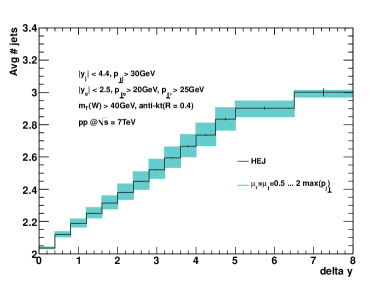
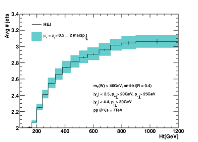
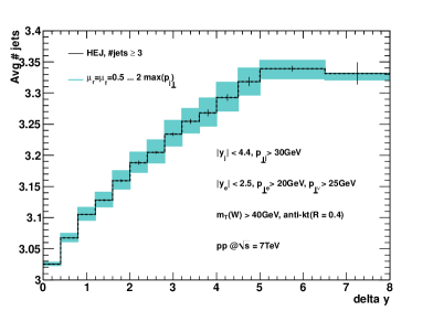
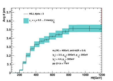
Figure 7: Top Left: The average number of jets as a function of the rapidity difference between the most forward and most backward jet and Top Right: the average number of jets as a function of $H_{T}$. Bottom Row: as top row, except restricted to events with 3 jets or more.

In Ref. [31], predictions for the average number of jets in $W+$dijet events were compared between four theoretical approaches: HEJ, a pure $Wjj$ NLO calculation[7, 6, 4], the “NLO exclusive sums” approach (a brute force method to combine NLO calculations of different orders) and the Sherpa[32, 33] MEPS[34, 35, 36] scheme which combines tree-level matrix elements of different orders in $\alpha_{s}$ with a truncated parton shower. Large differences were seen in the predictions between these theoretical descriptions and an experimental study of this variable would further our understanding of the nature of QCD radiation in the high-energy environment of the LHC.

The ratios of the inclusive jet rates are of course slightly less sensitive to additional radiation than the average number of jets. In Fig. 8 (top row) we plot the 3-jet to 2-jet rates, along with the ratio of the inclusive 4-jet to 3-jet rate (bottom row). Once again it is clear that the impact from higher orders in large. For illustration in the top row, the ratio between the tree-level 3-jet and 2-jet rates has also been plotted. Although this contains no systematic resummation of higher orders, in fact the leading-order result rises higher than that of HEJ.

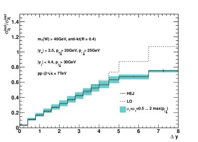
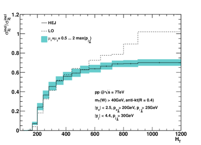
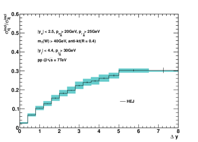
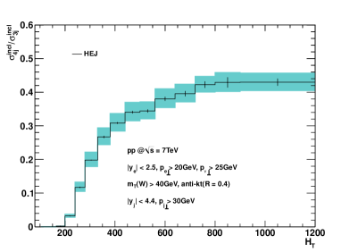
Figure 8: Top Left: The ratio between the inclusive 3-jet and 2-jet rates as a function of the difference in rapidity between the most forward and most backward jet; Top Right: The ratio of the inclusive 3-jet to 2-jet rate as function of $H_{T}$. The dotted line in each plot shows the ratio between the 3j and 2j tree-level calculations as a function of $\Delta y$ and $H_{T}$ respectively. Bottom Row: as top row, except the ratios are now of the inclusive 4-jet rate divided by the inclusive 3-jet rate.

The ratio of the inclusive 3-jet to 2-jet rate was also studied in Ref. [31] for the different theoretical descriptions listed above. As expected, smaller differences were seen between the approaches than in the predictions of the average number of jets, but even so, the experimental data could probably select a preferred description of the inclusive jet rates, especially at large $H_{T}$.

The ratio of the inclusive 4-jet to 3-jet rate is also shown in the bottom row of figure 8. The increase here is somewhat smaller than that seen for the ratio between the 3-jet and 2-jet-rates, but it still rises to 30% and 45% as a function of $\Delta y$ and $H_{T}$ respectively.

Finally, in Fig. 9 we compare the predictions from HEJ for the average number of jets vs. $\Delta y$ for inclusive $W+$dijets at the 7 TeV and the 8 TeV LHC.

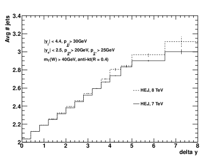
Figure 9: The average number of jets as a function of the rapidity span of each event (the difference in rapidity between the most forward and most backward jet) for 7 TeV and 8 TeV.

The result for 8 TeV shows only a very modest increase in the average number of jets.

In this section the predictions from HEJ for the average number of jets and ratios of inclusive jet rates have been shown. These show a large degree of sensitivity to additional hard QCD emissions beyond the leading order. These higher-order effects will only increase with the centre-of-mass energy of the LHC collisions.

6 Conclusions

We have described the application of the High Energy Jets (HEJ) framework to the production of a $W$ boson in association with at least two jets. HEJ resums systematically the contribution from multiple hard emissions (including also the leading virtual corrections). The process of $W+$dijets offers a key testing ground for our understanding of the behaviour of the Standard Model at the LHC, and will in turn be important for many directions including analyses of Higgs boson couplings and searches for new physics.

The predictions of HEJ were seen to give a very good description of the distributions studied with the 2010 data set. We further considered observables which are designed to be sensitive to the final state configuration of hard jets, and thus probe the perturbative description. We saw that the impact of higher orders on the inclusive dijet sample are large, for both the average number of jets and the ratios of inclusive jet rates in various regions of phase space. This offers the possibility of observing directly the impact of the BFKL-inspired resummation offered by HEJ.

The implementation of the formalism in the form of a fully flexible partonic Monte Carlo, can be downloaded at http://cern.ch/hej.

Higher order QCD effects have already been observed in data for pure jet production, and we look forward to future LHC analyses of $W$+jet production to further our understanding of physics at these new energy scales.

References

- [1] ATLAS Collaboration, G. Aad et al., Measurement of the production cross section for W-bosons in association with jets in pp collisions at sqrt(s) = 7 TeV with the ATLAS detector, Phys.Lett. B698 (2011) 325–345, [1012.5382].
- [2] ATLAS Collaboration, G. Aad et al., Study of jets produced in association with a W boson in pp collisions at sqrt(s) = 7 TeV with the ATLAS detector, 1201.1276.
- [3] CMS Collaboration, S. Chatrchyan et al., Jet Production Rates in Association with W and Z Bosons in pp Collisions at sqrt(s) = 7 TeV, 1110.3226.
- [4] C. Berger, Z. Bern, L. J. Dixon, F. Cordero, D. Forde, et al., Precise Predictions for W + 4 Jet Production at the Large Hadron Collider, Phys.Rev.Lett. 106 (2011) 092001, [1009.2338].
- [5] R. Ellis, K. Melnikov, and G. Zanderighi, W+3 jet production at the Tevatron, Phys.Rev. D80 (2009) 094002, [0906.1445].
- [6] C. Berger, Z. Bern, L. J. Dixon, F. Febres Cordero, D. Forde, et al., Precise Predictions for + 3 Jet Production at Hadron Colliders, Phys.Rev.Lett. 102 (2009) 222001, [0902.2760].
- [7] C. Berger, Z. Bern, L. J. Dixon, F. Febres Cordero, D. Forde, et al., Next-to-Leading Order QCD Predictions for W+3-Jet Distributions at Hadron Colliders, Phys.Rev. D80 (2009) 074036, [0907.1984].
- [8] R. Frederix, S. Frixione, V. Hirschi, F. Maltoni, R. Pittau, et al., aMC@NLO predictions for Wjj production at the Tevatron, 1110.5502.
- [9] S. Hoeche, F. Krauss, M. Schonherr, and F. Siegert, W+n-jet predictions with MC@NLO in Sherpa, 1201.5882. 4 pages, 1 table, 2 figures.
- [10] M. Rubin, G. P. Salam, and S. Sapeta, Giant QCD K-factors beyond NLO, JHEP 1009 (2010) 084, [1006.2144].
- [11] J. R. Andersen and J. M. Smillie, Constructing All-Order Corrections to Multi-Jet Rates, JHEP 1001 (2010) 039, [0908.2786].
- [12] J. R. Andersen and J. M. Smillie, The Factorisation of the t-channel Pole in Quark-Gluon Scattering, Phys.Rev. D81 (2010) 114021, [0910.5113].
- [13] J. R. Andersen and J. M. Smillie, Multiple Jets at the LHC with High Energy Jets, JHEP 1106 (2011) 010, [1101.5394].
- [14] ATLAS Collaboration, G. Aad et al., Measurement of dijet production with a veto on additional central jet activity in collisions at TeV using the ATLAS detector, JHEP 1109 (2011) 053, [1107.1641].
- [15] CMS Collaboration, S. Chatrchyan et al., Measurement of the inclusive production cross sections for forward jets and for dijet events with one forward and one central jet in collisions at TeV, 1202.0704.
- [16] CMS Collaboration Collaboration, S. Chatrchyan et al., Ratios of dijet production cross sections as a function of the absolute difference in rapidity between jets in proton-proton collisions at sqrt(s) = 7 TeV, 1204.0696.
- [17] V. S. Fadin, E. A. Kuraev, and L. N. Lipatov, On the Pomeranchuk singularity in asymptotically free theories, Phys. Lett. B60 (1975) 50–52.
- [18] E. A. Kuraev, L. N. Lipatov, and V. S. Fadin, Multi - Reggeon processes in the Yang-Mills theory, Sov. Phys. JETP 44 (1976) 443–450.
- [19] E. A. Kuraev, L. N. Lipatov, and V. S. Fadin, The Pomeranchuk singularity in nonabelian gauge theories, Sov. Phys. JETP 45 (1977) 199–204.
- [20] J. R. Andersen, V. Del Duca, F. Maltoni, and W. J. Stirling, W boson production with associated jets at large rapidities, JHEP 05 (2001) 048, [hep-ph/0105146].
- [21] J. R. Andersen, L. Lönnblad, and J. M. Smillie, A Parton Shower for High Energy Jets, JHEP 1107 (2011) 110, [1104.1316].
- [22] A. Martin, W. Stirling, R. Thorne, and G. Watt, Parton distributions for the LHC, Eur.Phys.J. C63 (2009) 189–285, [0901.0002].
- [23] J. R. Andersen and W. J. Stirling, Energy consumption and jet multiplicity from the leading log BFKL evolution, JHEP 02 (2003) 018, [hep-ph/0301081].
- [24] I. I. Balitsky and L. N. Lipatov, The Pomeranchuk singularity in quantum chromodynamics, Sov. J. Nucl. Phys. 28 (1978) 822–829.
- [25] B. L. Combridge and C. J. Maxwell, Untangling large p(t) hadronic reactions, Nucl. Phys. B239 (1984) 429.
- [26] J. R. Andersen and C. D. White, A New Framework for Multijet Predictions and its application to Higgs Boson production at the LHC, Phys. Rev. D78 (2008) 051501, [0802.2858].
- [27] J. R. Andersen, V. Del Duca, and C. D. White, Higgs Boson Production in Association with Multiple Hard Jets, JHEP 02 (2009) 015, [0808.3696].
- [28] J. Alwall et al., MadGraph/MadEvent v4: The New Web Generation, JHEP 09 (2007) 028, [0706.2334].
- [29] S. Catani, F. Krauss, R. Kuhn, and B. Webber, QCD matrix elements + parton showers, JHEP 0111 (2001) 063, [hep-ph/0109231].
- [30] L. Lönnblad, Ariadne version 4: A program for simulation of QCD cascades implementing the color dipole model, Comput. Phys. Commun. 71 (1992) 15–31.
- [31] J. A. Maestre, S. Alioli, J. Andersen, R. Ball, A. Buckley, et al., The SM and NLO Multileg and SM MC Working Groups: Summary Report, 1203.6803.
- [32] T. Gleisberg, S. Hoeche, F. Krauss, A. Schalicke, S. Schumann, et al., SHERPA 1. alpha: A Proof of concept version, JHEP 0402 (2004) 056, [hep-ph/0311263].
- [33] T. Gleisberg, S. Hoeche, F. Krauss, M. Schonherr, S. Schumann, et al., Event generation with SHERPA 1.1, JHEP 0902 (2009) 007, [0811.4622].
- [34] S. Hoeche, F. Krauss, S. Schumann, and F. Siegert, QCD matrix elements and truncated showers, JHEP 0905 (2009) 053, [0903.1219].
- [35] S. Hoeche, S. Schumann, and F. Siegert, Hard photon production and matrix-element parton-shower merging, Phys.Rev. D81 (2010) 034026, [0912.3501].
- [36] T. Carli, T. Gehrmann, and S. Hoeche, Hadronic final states in deep-inelastic scattering with Sherpa, Eur.Phys.J. C67 (2010) 73–97, [0912.3715].