Infrahumps detected in Kepler light curve of V1504 Cygni

Abstract

We present a power spectral density analysis of the short cadence Kepler data for the cataclysmic variable V1504 Cygni. We identify three distinct periods: the orbital period ($1.668\pm 0.006$ hours), the superhump period ($1.732\pm 0.010$ hours), and the infrahump period ($1.633\pm 0.005$ hours). The results are consistent with those predicted by the period excess-deficit relation.

1 Introduction

NASA’s Kepler mission has been providing high time-resolution optical photometry since its launch on March 6, 2009 (Koch et al., 2010). Designed to survey a fixed 105 square degree field of view, it monitors the brightness of over 100,000 stars primarily for the purpose of detecting and categorizing exoplanets. However, due to the extremely high quality of the instrument, it has proven itself a boon for other astronomical communities as well, including those interested in the study of Cataclysmic Variables (CVs).

CVs are classified based on their outburst properties, with the most active category being dwarf novae (DN). These systems are marked by quasi-periodic outbursts of varying strength, typically increasing in brightness by a few magnitudes. Dwarf novae are further separated into subtypes based on the manner in which these outbursts present themselves. SU UMa-type DN are characterized by the presence of occasional superoutbursts, dramatic eruptions several magnitudes brighter than normal outbursts. DN that do not exhibit such behavior are classified as U Gem-type.

Whether a system exhibits SU UMa or U Gem characteristics is dependent on the orbital dynamics of the system, and can be characterized by its mass ratio ($q=M_{2}/M_{1}$) and its orbital period (see Eq. 3). Each group tends to lie within separate distributions on either side of a critical mass ratio ($q_{\mathrm{crit}}\approx 0.33$). U Gem-type DN have long periods corresponding to mass ratios greater than the critical value ($q>q_{\mathrm{crit}}$) whereas SU UMa-type DN have shorter periods corresponding to mass ratios less than the critical value ($q<q_{\mathrm{crit}}$) (Hellier, 2001).

The Kepler field of view includes 10 CVs. Of the SU UMa-type, only V344 Lyra has been the subject of extensive study (Wood et al., 2011), and to date no equivalent treatment has been undertaken for V1504 Cygni, which is the object of interest in this paper. Like V344 Lyra, V1504 Cygni is a SU UMa-type dwarf novae, and as such features superoutbursts in addition to normal outburst behavior. Superhumps, periodic signals which are presumed to arise from the prograde precession of an elliptically elongated accretion disk (Hellier, 2001), have previously been identified in the V1504 light curves and studied in detail by Cannizzo et al. (2011).

A thorough analysis of the Kepler lightcurve of V1504 Cygni suggests the presence of negative superhumps (henceforth referred to by the shorter term infrahumps), as well. These are presumed to be associated with the nodal precession of a tilted accretion disk.

In this paper, we outline the process of identifying and extracting the period of these signals in Sec. 2, and then show that they are consistent with those predicted by the period excess-deficit relation in Sec. 3. We conclude with our main findings in Sec. 4.

2 Data Analysis

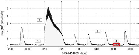
Figure 1: A segment of the SAP light curve for V1504 Cygni spanning from March 7, 2010 to June 15, 2010. Featured prominently in the center is the 5th superoutburst observed by Kepler. Notable features are (1) a superoutburst region with pronounced superhumps preceded by a shoulder with a profile matching a typical outburst, (2) outbursts that tend to gradually increase in magnitude, leading up to a superoutburst, (3) example data gap that would be corrected before periodicity analysis is performed, and (4) a five day window between 350 and 355 days that is used to generate the plots in Figures 3 and 4 as indicated in red.

The Kepler data used in this study are the Simple Aperture Photometry (SAP) photon fluxes recorded in the Kepler short cadence (SC) of approximately 1 minute. They are taken from a 550 day span starting on June 20, 2009 and lasting to December 22, 2010. A portion of the associated light curve is shown in Fig. 1.

Gaps in the data that correspond to monthly data downloads occur throughout the light curve, which if not treated properly can distort the temporal-resolution of the time-series or introduce anomalous structures in the associated power specta. These structures were ultimately eliminated through a correction process in which the gaps were filled with adjacent data, half from the left of each gap and half from the right. This has the benefit of reducing drastic oscillations in the high-frequency components of the power spectrum, enabling clearer recognition of peaks that correspond to physical frequencies of interest.

The improved clarity does not come without cost, however. When a longer gap (typically corresponding to scheduled data transfer or unexpected downtime) appears at the periphery of an outburst phase, part of the outburst is often copied into the gap, creating the appearance of a double-peak. This generates an artificial low-frequency contribution in the power spectrum for regions containing one of these gaps. This manifests in the power spectrum as intermittent vertical banding. This banding does not affect the identification or extraction of periodic signals in unaffected regions, and is therefore ignored for the purposes of this paper.

Once the SAP light curve was extracted from the Kepler data files and corrected for relevant artifacts, residuals were obtained by subtraction of a boxcar-smoothed version of the curve. This was done largely to eliminate saturation in the low-frequency spectrum during subsequent analyses, in order to emphasize the presence of higher frequency periodic signals associated with the orbital dynamics of the system.

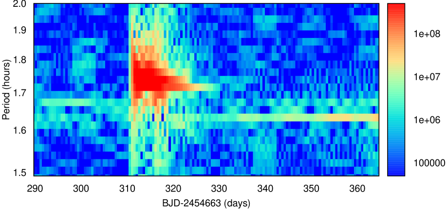
Figure 2: The power spectrum for the region of the light curve shown in Fig. 1, highest power output appears in red whereas the lowest appears in blue. The superoutburst that occurs near day 310 in Fig. 1 is associated with a dramatic increase in the contribution from confirmed superhumps. Two additional, weaker signals are indicated by the horizontal banding observed at periods of $\sim$1.67 and $\sim$1.63 hours. These are confirmed to be the orbital, and infrahump periods, respectively.

Following Still et al. (2010), the power spectrum (Fig. 2) was obtained from the residuals by Short-time Fourier transform (STFT), which here aggregates the power spectra over a 120 hour window, stepped across the duration of the light curve in 12 hour increments. Though there are no permanent periodic structures, there are three distinct signals that appear with varying degrees of persistence and intensity. The periods associated with each signal were obtained by extracting peak frequency values from the power spectrum (see Fig. 3). In addition, the extracted periods were confirmed by using a Levenberg-Marquardt non-linear least squares algorithm to fit a sinsoidal function to selected quiescent regions of the light curve (see Fig. 4).

The most dramatic feature in Fig. 2 is the presence of superhumps whose contributions dominate during the superoutburst phase. These occur when instabilities form during an outburst (hence the shoulder-like feature seen preceeding the superoutburst in Fig. 1), elongating the disk, which then begins to precess. These signals correspond to a period of $P_{\mathrm{sh}}=1.732\pm 0.010$ hours, in excellent agreement with the superhump period value measured by Antonyuk & Pavlenko (2005).

There is also evidence for two additional periodic signals that arise in the latter half of the power spectrum. We identify the weaker of these two signals, which becomes apparent approximately 200 days after the start of data acquisition, as the orbital period ($P_{\mathrm{o}}=1.668\pm 0.006$ hours), in good agreement with the value measured by Thorstensen & Taylor (1998). Once manifested, this signal persists throughout the remainder of the data set.

The second, stronger signal begins to contribute after approximately 250 days, and then intensifies, dominating the upper end of the frequency spectrum. It corresponds to a period of $P_{\mathrm{ih}}=1.633\pm 0.005$ hours. There is strong evidence that this period corresponds to infrahumps, as will be discussed in Sec. 3.

Table 1: Summary of salient results for V1504 Cyg.

Parameter	Symbol	Value (units)
Orbital period	$P_{\mathrm{o}}$	$1.668\pm 0.006$ (hours)
Superhump period	$P_{\mathrm{sh}}$	$1.732\pm 0.010$ (hours)
Infrahump period	$P_{\mathrm{ih}}$	$1.633\pm 0.005$ (hours)
Superhump period excess	$\epsilon_{+}$	$(3.84\pm 0.70)$%
Infrahump period deficit	$\epsilon_{-}$	$-(2.10\pm 0.47)$%
Mass ratio	$q$	$0.168\pm 0.044$
Secondary mass	$M_{2}$	$0.128\pm 0.050$ ($M_{\odot}$)
Roche lobe volume radius	$R_{2}/a$	$0.246\pm 0.022$
Apsidal precession period	$P_{\mathrm{ap}}$	$45.1\pm 8.1$ (hours)
Nodal precession period	$P_{\mathrm{no}}$	$77.8\pm 17.3$ (hours)

Figure 3: The power spectrum of the residuals for a 5 day window spanning from 350 to 355 (BJD-2454663) days, as indicated by the shaded box in Fig. 1. The peak at approximately 0.01 min^-1 corresponds to an infrahump period of $1.633\pm 0.005$ hours.

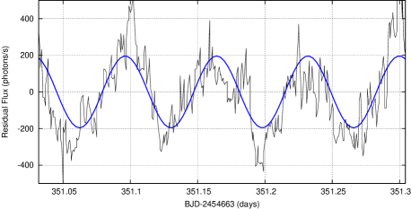
Figure 4: Example of the residual flux within the 350-355 (BJD-2454663) day window highlighted in Fig. 1. The resultant sinusoidal fit is overlaid in blue. The fit result for the infrahump period is $1.629\pm 0.024$ hours, in good agreement with the values extracted from the power spectrum.

3 Discussion

It is useful to discuss the nature of a dwarf nova’s orbital dynamics in terms of the so-called superhump period excess, defined as

$$\epsilon_{+}\equiv\frac{P_{\mathrm{sh}}-P_{\mathrm{o}}}{P_{\mathrm{o}}},$$ (1)

which is a measure of fractional apsidal precession. Patterson (1998) and Murray (2000) showed that this value is dependent on the mass ratio of the system, which itself can be recast in terms of the orbital period. This not only provides a useful metric for quantifying whether or not an observed periodic signal is associated with superhumps, but also for obtaining the mass-ratio due to the readily accessible measurement of orbital period. Using the formulation presented by Patterson (2005), the superhump period excess is related to the mass ratio of the binary system by

$$\epsilon_{+}=0.18q+0.29q^{2}.$$ (2)

With the assumed mass of a white dwarf ($M_{1}=0.76\pm 0.22~{}M_{\odot}$) and the Smith & Dhillon (1998) secondary mass-period relation

$$M_{2}\approx(0.038\pm 0.003)P_{o}^{(1.58\pm 0.09)}~{}M_{\odot},$$ (3)

it is straightforward to calculate the mass ratio from an observed orbital period. Here, the measured superhump period excess for V1504 results in a mass ratio of $q=0.1677\pm 0.0086$, well below the critical value that differentiates between SU UMa- and U Gem-type systems and is therefore required for the emergence of superhumps, confirming V1504’s classification. Likewise, an estimate for the mass of the secondary can be placed at $0.1275\pm 0.0375~{}M_{\odot}.$

The superhump period excess is also valuable for determining whether or not an observed periodic signal is associated with infrahumps. Defining the infrahump period deficit ($\epsilon_{-}$) in a manner identical to Eq. 1, one obtains a value related to the fractional nodal precession (negative since the precession is retrograde). This has been empirically shown by Patterson (1999) to be directly related to the superhump period excess by $\epsilon_{+}/\epsilon_{-}=-2.$ This relationship, along with Eq. 2 and Eq. 3, is used to plot the theoretical $\epsilon_{\pm}$ values for varying orbital periods, along with data from several other systems that display super- and infrahumps in Fig. 5. The measured value for the third periodic signal present in the power spectrum resides comfortably within the error bars associated with $\epsilon_{-}$, suggesting strongly that it is caused by infrahumps. Though this feature is not permanent, it does persist for a significant duration after manifesting, raising questions as to its source. Kato et al. (2012) suggest that such infrahumps may be the result of weak excitations of tidal instabilities in the disk that fail to trigger a superoutburst, which may imply a common origin for superhump and infrahump excitations.

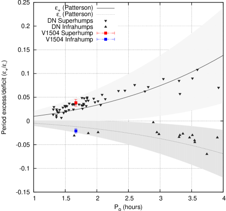
Figure 5: Theoretical dependence on orbital period for superhump period excess (solid line) and infrahump period deficit (dotted line) from Patterson (2005). The shaded regions associated with each line reflect the uncertainty in the values used in Eq. 3. Plotted as grey triangles are the values for superhumps using data from Patterson (1998) and infrahumps using a selection of data compiled by Wood, Thomas & Simpson (2009) from numerous sources. The V1504 values for superhump excess (red square) and infrahump deficit (blue square) are plotted accordingly, and fall comfortably within the error regions.

These results, along with additional calculated values for apsidal and nodal precession from formulae described in Hellier (2001) and the Roche lobe volume radius from formulae described in Smith & Dhillon (1998), are summarized in Table 1.

4 Conclusion

By examining the Kepler short cadence data for V1504 Cygni, we have identified three distinct periodic signals. Two of these are readily identifiable as the orbital period and the well-studied superhump period, each confirmed by independent measurements.

The presence of infrahumps in V1504 is inferred from the measurement of a third periodic signal in the power spectrum that corresponds to neither the established orbital period nor superhump period, and confirmed by comparison of the infrahump period deficit against empirical models. We have measured the infrahump period to be $1.633\pm 0.005$ hours.

5 ACKNOWLEDGEMENTS

The GW astro group is grateful for the help provided by Martin Still in the initial acquisition of some of the CV data.

References

- Antonyuk & Pavlenko (2005) Antonyuk, O.I., Pavlenko, E.P., 2005, SU UMa-type dwarf nova V1504 Cygni during several supercycles, ASP Conference Series, 330
- Cannizzo et al. (2011) Cannizzo J.K., Smale A.P., Wood M.A., Still M.D., Howell S.B., 2012, The Kepler light curves of V1504 Cygni and V344 Lyra: a study of the outburst properties, ApJ, 747, 117
- Hellier (2001) Hellier C., 2001, Cataclysmic Variable Stars, How and why they vary, Praxis Publishing, Chichester, UK
- Kato et al. (2012) Kato T. et al, 2012, Survey of Period Variations of Superhumps in SU UMa-Type Dwarf Novae. III: The Third Year (2010-2011), PASJ, 64, 21
- Koch et al. (2010) Koch D.G. et al, 2010, Kepler Mission Design, Realized Photometric Performance, and Early Science, ApJ, 713, L79
- Murray (2000) Murray J.R., 2000, The precession of eccentric discs in close binaries, MNRAS, 314, L1
- Patterson (1998) Patterson J., 1998, Late Evolution of Cataclysmic Variables, PASP, 110, 752
- Patterson (1999) Patterson J., 1999, in Mineshige S., Wheeler J.C., eds, in Disk Instabilities in Close Binary Systems, Kyoto: Universal Acad. Press, 61
- Patterson (2005) Patterson J. et al, 2005, Superhumps in Cataclysmic Binaries. XXV. , and Mass-Radius, PASP, 837, 117
- Smith & Dhillon (1998) Smith D.A., Dhillon V.S., 1998, The secondary stars in cataclysmic variables and low-mass X-ray binaries, MNRAS, 301, 767
- Still et al. (2010) Still M., Howell S.B., Wood M.A., Cannizzo J.K., Smale A.P., 2010, Quiescent superhumps detected in the dwarve nova V344 Lyra by Kepler, ApJ, 717, L113
- Thorstensen & Taylor (1998) Thorstensen J.R., Taylor C.J., 1998, Orbital Periods for the SU UMa-Type Dwarf Novae UV Persei, VY Aquarii, and V1504 Cygni, PASP, 109, 1359
- Wood, Thomas & Simpson (2009) Wood M.A., Thomas D.M., Simpson J.C., 2009, SPH Simulations of Negative (Nodal) Superhumps: A Parametric Study, MNRAS, 398, 2110
- Wood et al. (2011) Wood M.A., Still M.D., Howell S.B., Cannizzo J.K., Smale A.P., 2010, V344 Lyra: A touchstone SU UMa cataclysmic variable in the kepler field, ApJ, 741, 105