Using Synthetic Spacecraft Data to Interpret
Compressible Fluctuations in Solar Wind Turbulence

Abstract

Kinetic plasma theory is used to generate synthetic spacecraft data to analyze and interpret the compressible fluctuations in the inertial range of solar wind turbulence. The kinetic counterparts of the three familiar linear MHD wave modes—the fast, Alfvén, and slow waves—are identified and the properties of the density-parallel magnetic field correlation for these kinetic wave modes is presented. The construction of synthetic spacecraft data, based on the quasi-linear premise—that some characteristics of magnetized plasma turbulence can be usefully modeled as a collection of randomly phased, linear wave modes—is described in detail. Theoretical predictions of the density-parallel magnetic field correlation based on MHD and Vlasov-Maxwell linear eigenfunctions are presented and compared to the observational determination of this correlation based on 10 years ofWind spacecraft data. It is demonstrated that MHD theory is inadequate to describe the compressible turbulent fluctuations and that the observed density-parallel magnetic field correlation is consistent with a statistically negligible kinetic fast wave energy contribution for the large sample used in this study. A model of the solar wind inertial range fluctuations is proposed comprised of a mixture of a critically balanced distribution of incompressible Alfvénic fluctuations and a critically balanced or more anisotropic than critical balance distribution of compressible slow wave fluctuations. These results imply that there is little or no transfer of large scale turbulent energy through the inertial range down to whistler waves at small scales.

1 Introduction

Despite more than forty years of direct spacecraft measurements of turbulence in the near-Earth solar wind (Coleman, 1968), our understanding of turbulence in a magnetized plasma remains incomplete. One of the primary goals is to understand the role of the turbulence in mediating the transfer of energy from large to small scales. Within the turbulent inertial range of scales, corresponding to spacecraft-frame frequencies of $10^{-4}$ Hz $\lesssim f_{sc}\lesssim 1$ Hz or length scales $10^{6}$ km $\gtrsim\lambda\gtrsim 10^{2}$ km, the fluctuations involved in this energy transfer are a mixture of compressible and incompressible fluctuations, with around 90% of the energy in the incompressible component (Tu & Marsch, 1995; Bruno & Carbone, 2005). These incompressible fluctuations have been identifed as Alfvén waves (Belcher & Davis, 1971), but the nature of the compressible component remains uncertain.

The compressible turbulent fluctuations have often been interpreted as a combination of magnetoacoustic (fast MHD) waves and pressure-balanced structures (Tu & Marsch, 1995; Bruno & Carbone, 2005). Early studies of thermal and magnetic pressure fluctuations in the solar wind found an anti-correlation of the thermal pressure and magnetic pressure at timescales of 1 h, corresponding to an interval of constant total pressure, or a pressure-balanced structure (PBS) (Burlaga, 1968; Burlaga & Ogilvie, 1970). Further studies found evidence of PBSs out to 24 AU (Burlaga et al., 1990). Related investigations discovered a similar anti-correlation between the density $n$ and magnetic field magnitude $B$ from 0.3 AU to 18 AU on timescales ranging from several hours to 1.8 minutes (Vellante & Lazarus, 1987; Roberts et al., 1987a, b; Roberts, 1990). Theoretical studies of compressive MHD fluctuations in the low-Mach number, high-$\beta$ limit interpreted these anti-correlated density-magnetic field strength observations as nonpropagating “pseudosound” density fluctuations (Montgomery et al., 1987; Matthaeus et al., 1991). Later, a more comprehensive observational investigation confirmed the general density-magnetic field magnitude anti-correlation, but also identified a few positively correlated intervals consistent with the magnetosonic (fast MHD) wave (Tu & Marsch, 1994). Analysis of Ulysses observations found evidence for PBSs at inertial range scales in the high latitude solar wind (McComas et al., 1995; Reisenfeld et al., 1999; Bavassano et al., 2004). Studies of the electron density up to $f=2.5$ Hz also found pressure balanced structures but interpreted these as ion acoustic (slow MHD) waves and recognized that PBSs are simply the ion acoustic (slow MHD) wave in the perpendicular wavevector limit (Kellogg & Horbury, 2005), a fact previously noted by Tu & Marsch (1994). Recently, measurements of the anti-correlation between electron density and magnetic field strength indicated the existence of PBSs over timescales ranging from 1000 s down to 10 s (Yao et al., 2011).

An important consideration in the study of the compressible fluctuations of solar wind turbulence is the fact that the mean free path in the solar wind plasma is about 1 AU, so the dynamics over the entire inertial range is weakly collisional. The implications of this fact have not been seriously addressed in any of the aforementioned studies of compressible fluctuations in solar wind turbulence. The MHD description is rigorously valid only in the limit of strong collisionality, so a kinetic description is formally required to describe the inertial range turbulence. In the limit $k_{\parallel}\ll k_{\perp}$ predicted by anisotropic MHD turbulence theories (Goldreich & Sridhar, 1995; Boldyrev, 2006), it has been demonstrated that, even in the weakly collisional limit, the turbulent dynamics of the Alfvén waves decouples from the compressible fluctuations and is rigorously described by the equations of reduced MHD (Schekochihin et al., 2009). The compressible fast and slow wave modes, on the other hand, require a kinetic description to resolve both the wave dynamics and the collisionless kinetic damping mechanisms. The study presented here is the first to examine the properties of the compressible fluctuations in the turbulent solar wind using Vlasov-Maxwell kinetic theory. Specifically, we use the predicted correlation between the density fluctuations and parallel magnetic field fluctuations to determine the nature of the compressible fluctuations in the solar wind.

In §2, we explore the connection between the familiar linear wave modes in MHD and the corresponding kinetic wave modes in Vlasov-Maxwell kinetic theory and demonstrate that weakly collisional conditions do not change the qualitative properties of the density-parallel magnetic field correlation. In §3, we discuss the quasi-linear premise upon which the method of synthetic spacecraft data is based and describe in detail the procedure for generating synthetic spacecraft data. The synthetic spacecraft data predictions of the density-parallel magnetic field correlation based on linear MHD and Vlasov-Maxwell eigenfunctions is presented in §4. A comparison of the synthetic spacecraft data predictions to the observational determination of the density-parallel magnetic field correlation is presented in §5, showing a statistically negligible fast wave energy contribution to the compressible fluctuations. The implications of this finding are discussed before summarizing the findings of this investigation in §6.

2 Collisional vs. Collisionless Dynamics of Compressible Fluctuations

The inertial range of solar wind turbulence is observed to be a mixture of incompressible and compressible motions, with around 90% of the energy due to the incompressible component (Tu & Marsch, 1995; Bruno & Carbone, 2005). If these fluctuations are interpreted as some mixture of the three MHD linear wave modes, then Alfvén waves are responsible for the incompressible component, while slow and fast MHD waves make up the compressible component. In the limit of large scales compared to the thermal ion Larmor radius, $k\rho_{i}\ll 1$, these modes may be distinguished by the correlation between the density and parallel magnetic field fluctuations: fast waves are positively correlated, slow waves are negatively correlated, and the density and parallel magnetic field fluctuations are both zero for Alfvén waves. As the wave amplitude is increased to nonlinear levels, even in the limit that they form discontinuities or shocks, these qualitative properties persist, corresponding to tangential and rotational discontinuities or fast and slow shocks (Baumjohann & Treumann, 1996). In this section, we will explore the properties of the kinetic counterparts to the fast and slow MHD wave modes in the inertial range using Vlasov-Maxwell kinetic theory.

2.1 The Inertial Range Limit of the Compressible Linear Wave Modes

As derived in Appendix A, the normalized compressible MHD linear dispersion relation depends on only two parameters, $\omega/(kv_{A})=\overline{\omega}_{MHD}(\beta,\theta)$: the plasma beta, $\beta=c_{s}^{2}/v_{A}^{2}$, where the sound speed is $c_{s}=\sqrt{\gamma p_{0}/\rho_{0}}$ and the Alfvén velocity is $v_{A}=B_{0}/\sqrt{4\pi\rho_{0}}$; and the angle $\theta$ between the local mean magnetic field $\mathbf{B}_{0}$ and the direction of the wavevector.

To establish precisely the connection between the three linear MHD wave modes and their kinetic counterparts in the linear Vlasov-Maxwell system, we specify a fully-ionized proton and electron plasma with isotropic Maxwellian velocity distributions and a realistic mass ratio $m_{i}/m_{e}=1836$. In general, the linear Vlasov-Maxwell dispersion relation depends on five parameters: the ion plasma beta $\beta_{i}=8\pi n_{i}T_{i}/B_{0}^{2}$, which is the ratio of the ion thermal pressure to the magnetic pressure, the normalized wavenumber $k\rho_{i}$, the angle $\theta$ between the local mean magnetic field $\mathbf{B}_{0}$ and the direction of the wavevector, the ion to electron temperature ratio $T_{i}/T_{e}$, and the ratio of ion thermal velocity to the speed of light $v_{ti}/c$. The solution may then be expressed as $\omega=\omega_{VM}(\beta_{i},k\rho_{i},\theta,T_{i}/T_{e},v_{ti}/c)$ (Stix, 1992; Quataert, 1998; Howes et al., 2006). To connect to the single fluid theory of MHD, we take equal ion and electron temperatures, $T_{i}/T_{e}=1$. In the inertial range limit, $k\rho_{i}\ll 1$, and for the non-relativistic conditions appropriate to the solar wind, $v_{ti}/c\ll 1$, the normalized linear Vlasov-Maxwell dispersion relation simplifies to $\omega/(kv_{A})=\overline{\omega}_{VM}(\beta_{i},\theta)$. Since $\beta=\beta_{i}+\beta_{e}=\beta_{i}(1+T_{e}/T_{i})$, direct quantitative comparison between the solutions of the MHD and Vlasov-Maxwell linear dispersion relations is possible by choosing $\beta=2\beta_{i}$ (Howes, 2009).

The Vlasov-Maxwell solutions presented in this section use the parameters $k\rho_{i}=2.2\times 10^{-4}$, $\frac{v_{t_{i}}}{c}=10^{-4}$, and $T_{i}/T_{e}=1$, and employ a realistic mass ratio $m_{i}/m_{e}=1836$. The complex eigenfrequencies are solved numerically (Quataert, 1998; Howes et al., 2006) with Bessel function sums evaluated to 100 terms to ensure accurate results.

2.2 Connection between MHD and Vlasov-Maxwell Linear Wave Modes

Previous studies have compared the properties of linear Vlasov-Maxwell wave modes with the linear modes from two-fluid theory (Krauss-Varban et al., 1994) and Hall MHD (Howes, 2009). Here we restrict ourselves to establishing the connection between MHD wave modes and Vlasov-Maxwell wave modes in the inertial range limit, $k\rho_{i}\ll 1$. Due to the reduced parameter space of the Vlasov-Maxwell system in the inertial range limit, the comparison between the three linear MHD wave modes and their kinetic counterparts is concisely expressed by the use of normalized Freidrichs diagrams, polar plots of the wave phase velocity normalized to the Alfvén speed $\omega/(kv_{A})$ vs. polar angle $\theta$, as shown in Figure 1 for four values of $\beta_{i}$.

As discussed by Krauss-Varban et al. (1994), the identification of corresponding wave modes is complicated by the existence of a branch cut in the complex solution space of the Vlasov-Maxwell dispersion relation. At inertial range scales $k\rho_{i}\ll 1$, this branch cut exists only at small angles $\theta$; for wavevectors in the perpendicular limit, the kinetic fast, Alfvén, and slow modes are always easily distinguished. Therefore, we adopt the strategy that we label the modes according to their properties in the perpendicular wavevector limit, and retain those labels for the linear dispersion relation solutions as the angle is decreased from $\theta=90^{\circ}$ to $\theta=0^{\circ}$. Further discussion of the properties of the kinetic fast and slow wave modes at small angles $\theta$ is presented in Appendix B.

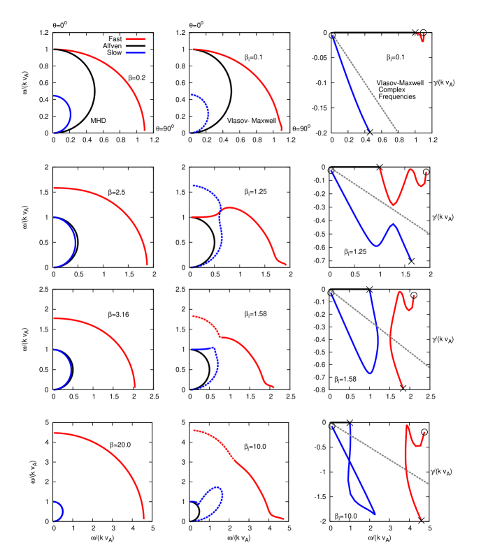
Figure 1: Fredrichs Diagrams of normalized phase speed $\omega/(kv_{A})$ for MHD (left column) and Vlasov-Maxwell (middle column) modes for $k\rho_{i}=2.2\times 10^{-4}$ and values of $\beta=2\beta_{i}=$ 0.2, 2.5, 3.16, and 20. Parallel wavevectors, $\theta=0^{\circ}$ with respect to the local mean magnetic field, lie along the the vertical axis, while perpendicular wavevectors, $\theta=90^{\circ}$, lie along the horizontal axis. Dashing indicates $-\gamma/\omega>0.25$, which implies heavy collisionless damping of that wave mode. On the right are the paths of the Vlasov-Maxwell solutions in complex $\omega$ space, running from the nearly parallel limit (crosses) to the nearly perpendicular limit (open circles), with $\gamma/\omega=-0.25$ plotted as a dashed grey line.

Results of the MHD to Vlasov-Maxwell comparison are presented in Figure 1. In the left column are the normalized Freidrichs diagrams for the MHD results for the fast wave (red), Alfvén wave (black), and slow wave (blue). In the center column are the Vlasov-Maxwell results for the kinetic fast wave (red), Alfvén wave (black), and kinetic slow wave (blue). Note that the strongly damped Vlasov-Maxwell modes (defined by $-\gamma/\omega>0.25$, where $\omega+i\gamma$ is the complex Vlasov-Maxwell eigenfrequency) are given by dashed lines. In the right column are the paths of the Vlasov-Maxwell solutions in complex $\omega$ space, running from the nearly parallel limit (crosses) to the nearly perpendicular limit (open circles). The region below the grey dashed line is $-\gamma/\omega>0.25$, indicating strong collisionless damping. Rows present different values for ion plasma beta, $\beta_{i}=0.1,1.25,1.58,10.0$.

For most values of $\beta_{i}$ and $\theta$ presented in the leftmost two columns of Figure 1, the correspondence between the MHD and kinetic wave modes is clear. It is worth noting, however, several distinctions between the fluid and kinetic behavior. First, the kinetic slow wave has a greater phase speed than the Alfvén wave for $\beta_{i}\gtrsim 1$. In fact, for sufficiently parallel wavevectors and $\beta_{i}\sim 1$, the kinetic slow mode also has a greater phase velocity than the fast mode. Second, the typical magnetic-to-acoustic mode conversion that occurs for the MHD fast and slow modes at $\beta=1$ is replaced by a conversion between the compressible kinetic roots at $\beta_{i}\sim 1.3$. This conversion leads to damping of the fast waves at small angles $\theta$ in the large $\beta_{i}$ limit. This general identification of the kinetic fast and slow wave modes is used in the construction of synthetic spacecraft data, as described in §3.

2.3 Density-Parallel Magnetic Field Correlation for Kinetic Fast and Slow Modes

With a clearly defined identification of the kinetic fast and slow modes complete, we may now calculate the density-parallel magnetic field correlation for the kinetic fast and slow modes. This will enable us to verify whether the general qualitative properties of this correlation—that fast waves are positively correlated, and slow waves negatively correlated—remain unchanged for collisionless conditions. The density fluctuation $\delta n$ and parallel magnetic field fluctuation $\delta B_{\parallel}$ may be calculated from the complex solution of the linear Vlasov-Maxwell dispersion relation. For a chosen wavevector $\mathbf{k}$, we obtain complex Fourier coefficients $\delta n(\mathbf{k})$ and $\delta B_{\parallel}(\mathbf{k})$, and we define the normalized correlation by Fourier mode, $C_{\mathbf{k}}$, given by

$$C_{\mathbf{k}}(\delta n,\delta B_{\parallel})=\mbox{Re}\left(\frac{\delta n(\mathbf{k})\delta B_{\parallel}(\mathbf{k})^{*}}{|\delta n(\mathbf{k})||\delta B_{\parallel}(\mathbf{k})|}\right).$$ (1)

Note here that the Fourier coefficients of both density and parallel magnetic field fluctuations satisfy the reality condition, e.g., $\delta n(\mathbf{k})=\delta n^{*}(-\mathbf{k})$.

In Figure 2, $C_{\mathbf{k}}(\delta n,\delta B_{\parallel})$ is plotted for the kinetic fast (left), Alfvén (center), and kinetic slow (right) modes as a function of the parameters $(\theta,\beta_{i})$. The remaining parameters for the Vlasov-Maxwell eigenfunction solutions are $k\rho_{i}=2\times 10^{-4}$, $T_{i}/T_{e}=1$, and $v_{t_{i}}/c=10^{-4}$. The kinetic fast mode (left) always has a positive correlation, with $C_{\mathbf{k}}(\delta n,\delta B_{\parallel})>0.9$ over most of the $(\theta,\beta_{i})$ plane. The kinetic slow mode (right) has a negative correlation with $C_{\mathbf{k}}(\delta n,\delta B_{\parallel})<-0.9$ over most of the $(\theta,\beta_{i})$ plane; the correlation becomes slightly positive for $\theta<30^{\circ}$ and $\beta_{i}\geq 1.3$. The Alfvén mode (center), presented for completeness, has a more complicated behavior, but it is worthwhile noting that the amplitudes of $\delta n(\mathbf{k})$ and $\delta B_{\parallel}(\mathbf{k})$ are both very small (compared to the characteristic amplitudes for either of the compressible waves) at inertial range scales, so this correlation for Alfvén waves is likely to be unmeasurable in the solar wind. In general, these results confirm that the general qualitative properties of the density-parallel magnetic field correlation remain unchanged for the kinetic fast, Alfvén, and slow modes in a weakly collisional plasma.

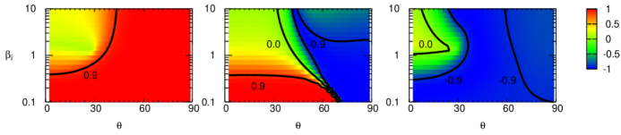
Figure 2: The normalized correlation by Fourier mode, $C_{\mathbf{k}}(\delta n,\delta B_{\parallel})$, for the kinetic fast (left), Alfvén (center), and slow (right) modes over the plane $(\theta,\beta_{i})$. A positive correlation is found for the kinetic fast modes, and a generally negative correlation for the slow modes.

3 Constructing Synthetic Spacecraft Data

The primary methodology employed in this study of the compressible fluctuations in the solar wind inertial range is the construction of synthetic spacecraft data for direct comparison to actual single-point spacecraft measurements. For the present study of the correlation between the density and parallel magnetic field fluctuations, this technique enables us to determine the characteristics of the correlation in the presence of a turbulent spectrum of wave modes. This method of analysis is based on the quasi-linear premise that some characteristics of magnetized plasma turbulence can be usefully modeled as a collection of randomly phased, linear wave modes; the justification for this premise is discussed in §3.1. The result from §2.1—that, in the inertial range, the dynamics of both MHD and Vlasov-Maxwell plasmas depend only on two parameters, the ion plasma beta $\beta_{i}$ and the wavevector angle $\theta$—significantly simplifies the construction of synthetic plasma data. Upon adoption of the quasi-linear premise and specification of the plasma $\beta_{i}$, one need only choose the partitioning of power among the contributing linear wave modes (fast, Alfvén, or slow) and the wavevector distribution of power (isotropic or critically balanced) for each of those modes, as described in §3.2.

3.1 The Quasi-linear Premise: Modeling Turbulence as a Spectrum of Linear Wave Modes

The theoretical investigation of turbulence using synthetic data is based on a concept that we denote the quasi-linear premise. The quasi-linear premise states that some properties of magnetized plasma turbulence can be understood by modeling the turbulence as a collection of randomly phased, linear waves. In this picture, the nonlinear turbulent interactions serve to transfer energy from one linear wave mode to another—thus, the picture is quasi-linear. The mathematical properties of the equations that describe turbulence in a magnetized plasma, in conjunction with a phenomonological understanding of the properties of the turbulence, provide the motivation for this quasi-linear approach. This concept can be most easily explained using the following example of turbulence in an incompressible MHD plasma.

The Elsasser form of the ideal incompressible MHD equations (Elsasser, 1950) is given by

$$\frac{\partial\mathbf{z}^{\pm}}{\partial t}\mp(\mathbf{v}_{A}\cdot\nabla)\mathbf{z}^{\pm}=-(\mathbf{z}^{\mp}\cdot\nabla)\mathbf{z}^{\pm}-\frac{\nabla p}{\rho_{0}},$$ (2)

where the magnetic field has been decomposed into its equilibrium and fluctuating parts $\mathbf{B}=\mathbf{B}_{0}+\delta\mathbf{B}$, the Alfvén velocity due to the equilibrium magnetic field $\mathbf{B}_{0}$ is given by $\mathbf{v}_{A}=\mathbf{B}_{0}/\sqrt{4\pi\rho_{0}}$, and $\mathbf{z}^{\pm}=\delta\mathbf{v}\pm\delta\mathbf{B}/\sqrt{4\pi\rho_{0}}$ are the Elsasser fields describing the velocity and magnetic field behavior of waves traveling down (up) the mean magnetic field. The second term on the left-hand side of equation (2) represents the linear propagation of the Elsasser fields along the mean magnetic field at the Alfvén speed, while the terms on the right-hand side represent the nonlinear interactions between upward and downward propagating waves, where the pressure gradient term ensures incompressibility of the fluctuations.

The theory of strong incompressible MHD turbulence (Goldreich & Sridhar, 1995; Boldyrev, 2006) suggests that the turbulent fluctuations at small scales become anisotropic, where the nonlinear cascade of energy generates turbulent fluctuations with smaller scales in the perpendicular direction than in the parallel direction, $k_{\parallel}\ll k_{\perp}$. This inherent anisotropy of magnetized plasma turbulence has long been recognized from early studies in laboratory plasmas (Robinson & Rusbridge, 1971; Zweben et al., 1979; Montgomery & Turner, 1981) and in early numerical simulations (Shebalin et al., 1983). It has been conjectured that strong turbulence in incompressible MHD plasmas maintains a state of critical balance between the linear timescale for Alfvén waves and the nonlinear timescale of turbulent energy transfer (Higdon, 1984; Goldreich & Sridhar, 1995). There exists significant evidence consistent with the predictions of critical balance from analysis of numerical simulations (Cho & Vishniac, 2000; Maron & Goldreich, 2001; Cho & Lazarian, 2003) and solar wind observations (Horbury et al., 2008; Podesta, 2009; Wicks et al., 2010; Luo & Wu, 2010; Chen et al., 2011; Forman et al., 2011). In a state of strong turbulence, critical balance implies that the linear term $(\mathbf{v}_{A}\cdot\nabla)\mathbf{z}^{\pm}$ and nonlinear term $(\mathbf{z}^{\mp}\cdot\nabla)\mathbf{z}^{\pm}$ in equation (2) are of the same order. It is this property that motivates the adoption of the quasi-linear premise, as discussed below.

In the absence of the nonlinear terms (setting the first term on the right-hand side of equation (2) to zero), the behavior of the plasma is entirely determined by the linear term. If the right-hand side of the equation is considered to be an arbitrary perturbing source term, the linear term determines the instantaneous response of the plasma to the imposed perturbation. In the case of weak turbulence (Sridhar & Goldreich, 1994; Montgomery & Matthaeus, 1995; Ng & Bhattacharjee, 1996; Goldreich & Sridhar, 1997; Ng & Bhattacharjee, 1997; Galtier et al., 2000; Lithwick & Goldreich, 2003), the nonlinear terms on the right-hand of equation (2) are indeed a small perturbation to the linear system, representing the nonlinear transfer of energy between the linear wave modes. Perturbation theory may be applied to the study of the turbulent dynamics in this limit, so the quasi-linear premise is clearly valid for the case of weak turbulence.

For strong turbulence, the condition of critical balance implies that the energy in a particular linear wave mode may be transferred nonlinearly to other modes on the timescale of its linear wave period. But since the linear and nonlinear terms are of the same order in critical balance, the linear term still contributes significantly to the instantaneous response of the plasma, even in the presence of strong nonlinearity. Therefore, the fluctuations in a strongly turbulent magnetized plasma are expected to retain at least some of the properties of the linear wave modes. In particular, for a turbulent fluctuation with a given wavevector, the amplitude and phase relationships between different components of that fluctuation are likely to be related to linear eigenfunctions of the characteristic plasma wave modes. In the construction of synthetic plasma turbulence data, a spectrum of randomly phased linear wave modes can be specified, with the amplitude of each of the linear modes adjusted to satisfy a chosen observational constraint, such as the turbulent magnetic energy spectrum (the second-order moment). By adopting the quasi-linear premise, the properties of the synthetic turbulence data may then be compared directly to spacecraft measurements to explore the nature of turbulent fluctuations.

The third- and higher-order moments of the turbulence, on the other hand, are clearly not described by this simplified quasi-linear approach. Such higher order statistics depend critically on the phase relationships between different linear wave modes, and these phase relationships are determined by the nonlinear interactions responsible for the turbulent cascade of energy from large to small scales. For a collection of randomly phased linear waves, such higher order statistics of synthetic data constructed using the quasi-linear premise will average to zero, yielding no useful information.

Although our illustration of the application of the quasi-linear premise above specifies the case of turbulence in an incompressible MHD plasma, the necessary general properties of the linear and nonlinear terms, as well as the inherent anisotropy of magnetized plasma turbulence, continue to hold for less restricted plasma conditions, including kinetic plasmas (Howes et al., 2006; Schekochihin et al., 2009). In particular, the arguments for the importance of the linear physics even in a strongly turbulent plasma also hold for the linear collisionless damping rates, providing the foundation for simple models of the turbulent energy cascade, encompassing both the inertial and dissipation ranges (Howes et al., 2008a, 2011).

Besides the feasibility arguments for the validity of the quasi-linear premise outlined above, we give here no a priori proof for its validity in strongly nonlinear plasma turbulence. Nonlinear simulations of plasma turbulence and observational studies of solar wind turbulence provide two avenues for testing the validity of the premise—at present, there exist arguments in the literature both for and against its validity. Analysis of nonlinear numerical simulations of plasma turbulence using gyrokinetics (Howes et al., 2008b, 2011) and both Hall MHD and Landau fluid theory (Hunana et al., 2011), as well as observational analysis of multi-spacecraft data in the solar wind (Sahraoui et al., 2010), support the validity of the quasi-linear premise. In addition, given that the idea of critical balance in strong MHD turbulence (Goldreich & Sridhar, 1995) is essentially a quasi-linear concept—that the timescale of the nonlinear energy transfer remains of order the linear wave frequency—evidence in support of critical balance (Cho & Vishniac, 2000; Maron & Goldreich, 2001; Cho & Lazarian, 2003; Horbury et al., 2008; Podesta, 2009; Wicks et al., 2010; Forman et al., 2011) also indirectly supports the quasi-linear premise. In contrast, studies of 3D incompressible MHD simulations (Dmitruk & Matthaeus, 2009) and 2D hybrid simulations (Parashar et al., 2010) of plasma turbulence, as well as an observational analysis of multi-spacecraft data in the solar wind (Narita et al., 2011), have called into question the validity of the quasi-linear premise. A review of this supporting and conflicting evidence for the quasi-linear premise is presented in Howes et al. (2011), focusing in particular on questionable aspects of the conflicting studies that cast doubt on the validity of their conclusion that the quasi-linear premise is inapplicable to the case of strong plasma turbulence.

It is also important to note that the utility of the quasi-linear premise for the study of plasma turbulence, however, may also be judged a posteriori by the insights gained from such an approach.

3.2 Procedure for Constructing Synthetic Spacecraft Data

Upon adopting the quasi-linear premise, the construction and analysis of synthetic spacecraft data requires three steps:

1. Populate a synthetic plasma volume with a spectrum of linear wave modes with a chosen distribution of power in wavevector space.

2. Sample the synthetic plasma volume at the position of a probe moving with respect to the plasma to generate reduced time series comparable to single-point spacecraft measurements.

3. Perform the requisite analysis on the synthetic time series to compare to spacecraft data analysis, for example, the zero-lag cross-correlation of the density and parallel magnetic field fluctuations.

For the study of the density and parallel magnetic field correlation of the solar wind compressible turbulent fluctuations, each of these steps is detailed below.

3.2.1 Creating the Synthetic Turbulent Plasma

As discussed in §2.1, for the inertial range of solar wind turbulence, the appropriately normalized linear physics of both the MHD (collisional fluid) and Vlasov-Maxwell (collisionless kinetic) systems depends on a reduced set of two parameters: the ion plasma beta $\beta_{i}$ and the wavevector angle $\theta$. Therefore, a completely general synthetic turbulent plasma requires the specification of just three properties: (1) the plasma beta, (2) the fraction of power in each of the possible linear wave modes, and (3) the distribution of power in wavevector space for each of these wave modes. Both observational constraints and phenomenological models of plasma turbulence guide our choices for these properties.

First, we discretize the three-dimensional wavevector space on a uniform grid of $32^{3}$ points, where each wavevector component spans $k_{i}\rho_{i}\in[-4.8\times 10^{-2},4.8\times 10^{-2}]$ with a minimum grid spacing $k_{0}\rho_{i}=3\times 10^{-3}$. Taking an equilibrium magnetic field $\mathbf{B}_{0}=B_{0}\mbox{$\hat{\mathbf{z}}$}$ and specifying the ion plasma beta $\beta_{i}$, we may solve for the normalized linear frequencies $\overline{\omega}(\mathbf{k})$ and the linear eigenfunctions $\delta\mathbf{B}(\mathbf{k}),\delta\mathbf{E}(\mathbf{k}),\delta\mathbf{U}(\mathbf{k}),\delta n(\mathbf{k})$ for each wavevector $\mathbf{k}$ using our chosen plasma description (MHD or Vlasov-Maxwell). Note that we adopt the convention $\omega\geq 0$, so that the direction of the wave group velocity (in the case of Alfvén waves, up or down the mean magnetic field) is determined by the wavevector.

Next, we specify the fraction of the turbulent magnetic power for each Fourier component due to the combination of the fast, Alfvén, and slow waves. After specifying the parititioning of turbulent power among the linear wave modes, we adjust the amplitudes of the Fourier coefficients of the linear wave modes so that the fluctuating magnetic power $|\delta\mathbf{B}(k)|^{2}$ (due to the linear superposition of all of the contributing wave modes at a given wavenumber $k$) is consistent with the inertial range observational constraint that the one-dimensional magnetic energy spectrum scales as $E_{B}\propto k^{-5/3}$. The amplitudes of the Fourier coefficients for the remaining fields $\delta\mathbf{E}(\mathbf{k})$, $\delta\mathbf{U}(\mathbf{k})$, and $\delta n(\mathbf{k})$ are specified by the eigenfunction solution of each of the linear wave modes. Random phases are also applied to each wave mode.

Finally, the distribution of energy in wavevector space for each of the constituent wave modes must be specified to model the inherently anisotropic nature of magnetized plasma turbulence. Imbalance between the turbulent energy fluxes propagating up and down the magnetic field as well as anisotropy in the angular distribution of turbulent energy with respect to the mean field direction may be incorporated in this final step. For this initial synthetic data investigation of the compressible fluctuations in the inertial range, we always set the upward and downward propagating wave energy fluxes in balance. Numerical simulations of compressible MHD plasma turbulence suggest that fast wave energy is distributed isotropically while both the Alfvén and slow wave energies obey a critically balanced distribution with energy concentrated mainly in modes with $k_{\parallel}\lesssim k_{0}^{1/3}k_{\perp}^{2/3}$, where $k_{0}$ is the isotropic driving scale of the turbulence (Cho & Lazarian, 2003). Therefore, we allow for two possible wavevector distributions of energy: (a) an isotropic distribution, such that the distribution of power is independent of $\theta$; and, (b) a simplified critically balanced distribution, where all modes with $k_{\parallel}>k_{0}^{1/3}k_{\perp}^{2/3}$ are set to zero, where $k_{0}$ is the minimum wavenumber of the simulation domain.

Note that the adjustment of the fraction of turbulent power due to each wave mode is performed for each Fourier component, so that changes in the wavevector distribution of energy—e.g., from isotropic to critically balanced by zeroing out all modes with $k_{\parallel}>k_{0}^{1/3}k_{\perp}^{2/3}$—do not affect the fluctuation amplitudes of the non-zero modes.

3.2.2 Generating Synthetic Reduced Time Series

Once the synthetic turbulent plasma has been completely specified in the Fourier domain, the turbulent fields may be computed at any position $\mathbf{r}$ and time $t$ by summing over all contributing Fourier modes of all constituent linear waves, for example,

$$\delta B_{\parallel}(\mathbf{r},t)=\sum_{m}\sum_{\mathbf{k}}\delta B_{\parallel m}(\mathbf{k})e^{i[\mathbf{k}\cdot\mathbf{r}-\omega_{m}(\mathbf{k})t+\phi_{mj}]}.$$ (3)

Here, the index $m$ indicates the contributions from fast, Alfvén, and slow modes, and each contributing Fourier mode $\mathbf{k}$ for each wave mode $m$ is given a constant, random phase $\phi_{mj}$, where $j=1,\ldots,n_{x}n_{y}n_{z}$. Note that the linear frequency $\omega_{m}(\mathbf{k})$ for each constituent wave is a function of the wavevector $\mathbf{k}$ as well as the wave type $m$.

Unfortunately, single-point satellite measurements do not provide full spatial information about the turbulence for comparison to the synthetic data. To mimic spacecraft measurements made as the super-Alfvénic solar wind streams past the satellite with velocity $\mathbf{v}$, we sample the synthetic plasma volume at the position of a probe moving with velocity $-\mathbf{v}$ through the volume, $\mathbf{r}(t)=\mathbf{r}_{0}-\mathbf{v}t$, where for simplicity we set $\mathbf{r}_{0}=0$. Sampling along the probe trajectory at an interval $\Delta t$ generates single-point time series at times $t_{n}=n\Delta t$ for each of the turbulent fluctuating fields, where $n=1,\ldots N$ and the total time interval is therefore $T=N\Delta t$. This reduced set of data is directly comparable to single-point spacecraft measurements. The time series of the parallel magnetic field fluctuation $\delta B_{\parallel n}\equiv\delta B_{\parallel}(t_{n})$, for example, is given by

$$\delta B_{\parallel n}=\left.\delta B_{\parallel}(\mathbf{r},t)\right|_{\mathbf{r}=-\mathbf{v}t_{n}}=\sum_{m}\sum_{\mathbf{k}}\delta B_{\parallel m}(\mathbf{k})e^{-i[(\mathbf{k}\cdot\mathbf{v}+\omega_{m})t_{n}-\phi_{mj}]}.$$ (4)

Note that the frequency $\omega^{\prime}$ of the signal measured by the moving probe is Doppler shifted by the probe velocity, $\omega^{\prime}=\omega+\mathbf{k}\cdot\mathbf{v}$. Normalizing this Doppler-shifted frequency by $kv_{A}$ to obtain $\overline{\omega}^{\prime}=\omega^{\prime}/(kv_{A})$, we find $\overline{\omega}^{\prime}=\overline{\omega}+\hat{\mathbf{k}}\cdot(\mathbf{v}/v_{A})$, where $\hat{\mathbf{k}}$ is the unit vector in the direction of the wave vector. The Taylor hypothesis—that the temporal fluctuations measured in the super-Alfvénic solar wind flow are dominated by spatial fluctuations swept past the probe at the solar wind velocity—is equivalent to the limit $\hat{\mathbf{k}}\cdot(\mathbf{v}/v_{A})\gg\overline{\omega}$ (Taylor, 1938). Because the ratio $v/v_{A}\simeq 10$ in the super-Alfvénic solar wind flow (Tu & Marsch, 1995; Bruno & Carbone, 2005), the Taylor hypothesis is frequently a useful simplification for studies of the non-dispersive linear wave modes of the inertial range. For the present study of the compressible fluctuations in the inertial range, we adopt the Taylor hypothesis that $\omega^{\prime}\simeq\mathbf{k}\cdot\mathbf{v}$, so

$$\delta B_{\parallel n}=\sum_{m}\sum_{\mathbf{k}}\delta B_{\parallel m}(\mathbf{k})e^{-i[\mathbf{k}\cdot\mathbf{v}t_{n}-\phi_{mj}]}.$$ (5)

In §4.5, we test the effect that violation of the Taylor hypothesis has on the density-parallel magnetic field correlation $C(\delta n,\delta B_{\parallel})$.

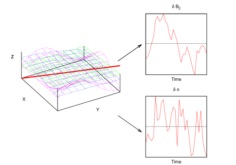
Figure 3: Probe trajectory (red) through a synthetic turbulent plasma volume generated using a spectrum of linear eigenfunctions (blue, green, and purple surface plots on the left). Measurements of the plasma fluctuations along the probe trajectory yield synthetic single-point time series of the parallel magnetic field fluctuation $\delta B_{\parallel}$ (upper right) and the density fluctuation $\delta n$ (lower right).

This procedure of sampling the synthetic plasma volume is depicted schematically in Figure 3. Here the blue, green, and purple surface plots represent the spatial variation for a few of the contributing Fourier modes to the turbulent fields. The synthetic plasma volume is sampled at uniform time intervals along the probe trajectory (red line), generating single-point time series of the parallel magnetic field fluctuation $\delta B_{\parallel n}$ (upper right) and the density fluctuation $\delta n_{n}$ (lower right). These synthetic time series may then be analyzed using the same procedures as the actual spacecraft measurements.

3.2.3 Analysis of Synthetic Spacecraft Data

As discussed in §2.3, the correlation between the density fluctuation $\delta n$ and the parallel magnetic field fluctuation $\delta B_{\parallel}$ distinguishes fast from slow compressible modes in either the fluid MHD or kinetic Vlasov-Maxwell systems. The zero-lag cross-correlation of the two time series $\delta n_{n}$ and $\delta B_{\parallel n}$ is given by

$$C(\delta n,\delta B_{\parallel})=\frac{\sum_{n}\left(\delta n_{n}-\overline{\delta n}\right)\left(\delta B_{\parallel n}-\overline{\delta B_{\parallel}}\right)}{\sqrt{\sum_{n}\left(\delta n_{n}-\overline{\delta n}\right)^{2}}\sqrt{\sum_{n}\left(\delta B_{\parallel n}-\overline{\delta B_{\parallel}}\right)^{2}}},$$ (6)

where $\overline{\delta n}$ and $\overline{\delta B_{\parallel}}$ are the averages over the time interval $T$. Comparison of the theoretical predictions of $C(\delta n,\delta B_{\parallel})$ to the correlation from spacecraft measurements, assuming the validity of the quasi-linear premise, provides a means of constraining the nature of the compressible fluctuations in the solar wind.

4 Theoretical Predictions of $C(\delta n,\delta B_{\parallel})$ Using Synthetic Spacecraft Data

Our theoretical investigation of the compressible fluctuations in the inertial range of solar wind turbulence uses the method outlined in §3 to generate synthetic spacecraft data to provide predictions of the density-parallel magnetic field correlation $C(\delta n,\delta B_{\parallel})$ as a function of the following turbulent plasma properties: the plasma $\beta_{i}$, the fraction of fast-to-total compressible wave power $\mathcal{F}$, and the angular distribution of the turbulent power in wavevector space. These theoretical predictions may then be compared directly to the $C(\delta n,\delta B_{\parallel})$ computed from satellite measurements to constrain the nature of the compressible fluctuations.

Below we present a comparison of four methods to predict and interpret the behavior of $C(\delta n,\delta B_{\parallel})$ as a function of $\beta_{i}$ and $\mathcal{F}$: (1) an analytical estimate using MHD eigenfunctions; (2) synthetic spacecraft data using MHD eigenfunctions, including contributions from fast, Alfvén, and slow waves; (3) synthetic spacecraft data using Vlasov-Maxwell eigenfunctions using only the compressible kinetic fast and slow waves; and (4) synthetic spacecraft data using Vlasov-Maxwell eigenfunctions, including contributions from fast, Alfvén, and slow waves. For each of these cases, we explore three combinations of the angular distribution of the constituent wave mode power: (a) all isotropically distributed wave power distributions, (b) all critically balanced wave power distributions, and (c) isotropic fast wave and critically balanced Alfvén and slow wave power distributions. Based on intuition gained from numerical simulations of compressible MHD turbulence (Cho & Lazarian, 2003), we expect that the third case of isotropic fast waves and critically balanced Alfvén and slow waves is the most realistic choice; the alternative selections are included to demonstrate the sensitivity of the method to different power distributions in wavevector space.

All of the synthetic spacecraft data results of $C(\delta n,\delta B_{\parallel})$ in this section are relatively insensitive to the angle of the probe trajectory with respect to the equilibrium magnetic field, as long as the trajectory is not exactly parallel or perpendicular to the field; all results here used an angle of $45^{\circ}$ with respect to both the equilibrium magnetic field and the $x$-axis. As a test of the validity of the Taylor hypothesis, we created sets of syntehtic data from a time evolving plasma in which the Taylor hypothesis is not assumed. The time evolution of each Fourier component for each wave mode was prescribed by its linear frequency and the rate of time evolution is parametrized by the ratio of solar wind to Alfvén velocities $v/v_{A}$. The correlation $C(\delta n,\delta B_{\parallel})$ from the time evolved and stationary cases were indistinguishable as long as the motion is sufficiently super- Alfvénic ($v/v_{A}\gtrsim 10$), which is typically satisfied in the solar wind (Tu & Marsch, 1995; Bruno & Carbone, 2005). Therefore, we assume the Taylor hypothesis is valid and present results derived from stationary synthetic data sets. For each choice of $\beta_{i}$ and $\mathcal{F}$, the values of $C(\delta n,\delta B_{\parallel})$ plotted in Figure 4 are the mean of 256 ensembles; the error bars are the standard deviation from this statistical averaging procedure. The ensembles are used to average over the random phases of the fluctuations.

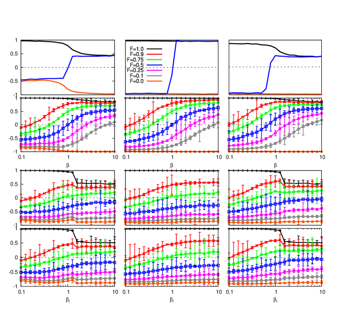
Figure 4: Theoretical predictions of $C(\delta n,\delta B_{\parallel})$ using synthetic spacecraft data as a function of ion plasma beta $\beta_{i}$ and fast-to-total compressible wave power $\mathcal{F}$. By row are analytical predictions based on MHD eigenfunctions (first), synthetic spacecraft data using MHD eigenfunctions (second), synthetic spacecraft data using Vlasov-Maxwell eigenfunctions with only fast and slow waves (third), and synthetic spacecraft data using Vlasov-Maxwell eigenfunctions with 90% Alfvén wave power, and the remaining wave power split between fast and slow waves (fourth). By column are presented different angular distributions of wave power: all isotropic (first), all critically balanced (second), isotropic fast and critically balanced Alfvén and slow (third). Results are presented for varying fractions of fast-to-total compressible wave power $\mathcal{F}$: 1.0 (black), 0.9 (red), 0.75 (green), 0.5 (blue), 0.25 (magenta), 0.1 (grey), 0.0 (orange). The error bars are the standard deviation from each ensemble of runs.

4.1 Analytical Estimate of $C(\delta n,\delta B_{\parallel})$

To build our intuition about the behavior of $C(\delta n,\delta B_{\parallel})$ for turbulence modeled as a spectrum of randomly phased linear wave modes, we use the normalized compressible MHD eigenfunctions presented in Appendix A to construct an analytical estimator $\Xi(\beta)$ for $C(\delta n,\delta B_{\parallel})$. For a plasma with an equilibrium magnetic field $\mathbf{B}_{0}=B_{0}\mbox{$\hat{\mathbf{z}}$}$, the density and parallel magnetic field fluctuation for a Fourier mode with wavevector $\mathbf{k}=k\sin\theta\mbox{$\hat{\mathbf{x}}$}+k\cos\theta\mbox{$\hat{\mathbf{z}}$}$ are generally given by the normalized Fourier coefficients $\delta\hat{n}(\beta,\theta)$ and $\delta\hat{B}_{\parallel}(\beta,\theta)$. We can estimate the correlation by integrating the correlations of the Fourier coefficients over the specified angular distributions of power for each wave mode,

$$\Xi(\beta)=\frac{\int\sum_{m}\left[\delta\hat{n}_{m}(\beta,\theta)\right]\sum_{m}\left[\delta\hat{B}_{\parallel m}(\beta,\theta)\right]d\theta}{\sqrt{(\int\sum_{m}\left[\delta\hat{n}_{m}(\beta,\theta)\right]d\theta)^{2}}\sqrt{(\int\sum_{m}\left[\delta\hat{B}_{\parallel m}(\beta,\theta)\right]d\theta)^{2}}},$$ (7)

where the sum over $m$ includes the contribution from each of the constituent wave modes. The expected dependence on $\beta$ is explicit in the expression, while the choice of mode fraction $\mathcal{F}$ is implicit in the choice of the fraction of power in each of the contributing wave modes. Since the Alfvén wave mode in the MHD limit has Fourier coefficients $\delta\hat{n}=\delta\hat{B}_{\parallel}=0$, it is unnecessary to include a contribution from Alfvén waves to the estimated correlation $\Xi(\beta)$. In the top row of Figure 4, $\Xi(\beta)$ is plotted for the three angular power distribution cases: all isotropic (left), all critically balanced (center), and isotropic fast and critically balanced slow (right). For each case, we compute the estimator $\Xi(\beta)$ for three fractions of fast-to-total compressible wave power $\mathcal{F}=0$ (orange), $\mathcal{F}=0.5$ (blue), and $\mathcal{F}=1$ (black).

Two qualitative features are immediately apparent from the top row of Figure 4. First, the behavior for the mixture of fast and slow modes is dominated by the slow mode in the $\beta<1$ region and by the fast mode in the $\beta>1$ region. This result can be understood by comparing the magnitude of the fast and slow mode density fluctuations in these regions. In the small $\beta$ region, the slow mode density fluctuations are one to two orders of magnitude larger than the fast mode fluctuations; the opposite case holds for the high $\beta$ region, where the density fluctuations for the fast mode are much larger than for the slow mode. Second, for the case of both isotropic wave power distributions (left), we see a dependence on $\beta$ both for pure fast modes at $\beta\gtrsim 1$ and for pure slow modes at $\beta\lesssim 1$. Noting that these pure modes have practically no $\beta$ dependence for the critical balance case (center), we can surmise that the parallel modes are the cause of the deviations seen in the isotropic case. The case of the combination of isotropic fast and critically balanced slow modes (right) appears to confirm this finding because the $\beta\lesssim 1$ (slow-wave dominated) region looks like the purely critically balanced case, while the $\beta\gtrsim 1$ (fast-wave dominated) region appears very much like the purely isotropic case. These qualitative characteristics of the analytical estimator $\Xi(\beta)$ for $C(\delta n,\delta B_{\parallel})$ provide a foundation upon which to interpret the synthetic spacecraft data predictions.

4.2 Synthetic Spacecraft Data Prediction of $C(\delta n,\delta B_{\parallel})$ using MHD Fast, Alfvén, and Slow Eigenmodes

The compressible MHD eigenfunctions presented in Appendix A are used in the procedure outlined in §3 to generate synthetic spacecraft data to theoretically predict the behavior of $C(\delta n,\delta B_{\parallel})$ as a function of the synthetic turbulent plasma properties. The synthetic plasma volume is sampled at $N=32$ uniformly spaced points along a trajectory of length $L=vT=\frac{2\pi}{3}\times 10^{3}\rho_{i}$. Although the MHD Alfvén wave has $\delta\hat{n}=\delta\hat{B}_{\parallel}=0$, the Alfvén wave contribution to the synthetic turbulent plasma is included for completeness, with 90% of the turbulent magnetic power given by incompressible Alfvén waves. The remaining 10% of the magnetic power is split between the MHD fast and slow waves according to the specified fraction of fast-to-total compressible wave power $\mathcal{F}$. Tests have shown that the results for $C(\delta n,\delta B_{\parallel})$ using MHD eigenfunctions are unaffected by the presence or absence of the Alfvén wave contribution, as expected. The resulting zero-lag cross correlation of the density and parallel magnetic field $C(\delta n,\delta B_{\parallel})$ from the synthetic MHD plasma is presented in the second row of Figure 4.

We see that $C(\delta n,\delta B_{\parallel})$ from the MHD synthetic data displays the same qualitative behavior as the analytical estimate $\Xi(\beta)$. The dominance in the low (high) $\beta$ regions by the slow (fast) mode behavior is evident. A plasma that has 90% of its compressive energy in the fast mode has a slightly negative correlation at $\beta=0.1$, while a 90% slow mode plasma has a small but positive correlation for $\beta=10$. Both of these values are drastically different from $C(\delta n,\delta B_{\parallel})$ at $\beta=1.0$. This dominant behavior holds true for all three choices of power distributions. In comparing the results from these distributions, we see the marked, and expected, lack of $\beta$ dependence for the pure fast and slow modes in the critical balance cases.

4.3 Synthetic Spacecraft Data Prediction of $C(\delta n,\delta B_{\parallel})$ using only Kinetic Fast and Slow Vlasov-Maxwell Eigenmodes

Unlike the MHD case, the Alfvén wave in the Vlasov-Maxwell kinetic theory has a small but non-zero fluctuating density and parallel magnetic field component in the inertial range limit, $k\rho_{i}\ll 1$. To illuminate the contribution of each of the linear kinetic wave modes to $C(\delta n,\delta B_{\parallel})$, in this section we generate a synthetic plasma consisting of a spectrum of only kinetic fast and slow wave fluctuations; in the next section, the (mostly incompressible) Alfvénic contribution will be included for completeness.

The sampling of the synthetic plasma volume is the same as for the MHD case, using $N=32$ and $L=\frac{2\pi}{3}\times 10^{3}\rho_{i}$. Numerical computation of the linear Vlasov-Maxwell eigenfunctions uses the parameters $T_{i}/T_{e}=1$, $\frac{v_{t_{i}}}{c}=10^{-4}$, and $m_{i}/m_{e}=1836$, with Bessel function sums evaluated to 100 terms to ensure accurate results (Quataert, 1998; Howes et al., 2006). We have assumed isotropic Maxwellian distribution functions for protons and electrons for all Vlasov-Maxwell synthetic spacecraft data results presented in this paper; further exploration of anisotropic temperature distributions may prove fruitful but is beyond the scope of the present work.

The results for $C(\delta n,\delta B_{\parallel})$ from the Vlasov-Maxwell synthetic plasma with only kinetic fast and slow waves are presented in the third row of Figure 4. Comparing to the MHD results (second row), we note an apparent similarity in the qualitative behavior but also some noticeable quantitative differences. First, the slow mode dominance in the $\beta_{i}\lesssim 1$ region is still observed for the kinetic plasma, but the $\beta_{i}\gtrsim 1$ region is not dominated by the fast mode as in the MHD case. In fact, the mixed modes have very little dependence on $\beta_{i}$ for $\beta_{i}\gtrsim 1.3$. Second, for pure fast and slow modes, the correlation for the isotropic case (left) does have a $\beta_{i}$ dependence in the high and low $\beta_{i}$ regions respectively, as is seen in the MHD case. However, for the pure slow mode, $C(\delta n,\delta B_{\parallel})$ is never perfectly anti-correlated, reaching a minimum value of $\simeq-0.9$. Third, as with the MHD plasma, the pure fast modes are perfectly correlated in the low $\beta_{i}$ region and become drastically less correlated for $\beta_{i}$ values above the mode conversion (see Appendix B) at $\beta_{i}\simeq 1.3$.

4.4 Synthetic Spacecraft Data Prediction of $C(\delta n,\delta B_{\parallel})$ using Kinetic Fast, Alfvén, and Slow Vlasov-Maxwell Eigenmodes

In this section, we incorporate an Alfvén wave contribution composing 90% of the turbulent magnetic power into the turbulent synthetic plasma, with the remaining 10% split between the kinetic fast and slow modes. Note that the total compressible wave power used to calculate $\mathcal{F}$ includes only the kinetic fast and slow wave contributions and does not include the small contribution to the compressible energy from the Alfvén wave. Since the density and parallel magnetic field fluctuations of the Alfvén wave both have small amplitudes, it is expected that the addition of the Alfvénic component will not yield significant quantitative changes in $C(\delta n,\delta B_{\parallel})$.

Sampling of the synthetic plasma volume and computation of the linear Vlasov-Maxwell eigenfunctions is the same as in the previous section. The resulting $C(\delta n,\delta B_{\parallel})$ for the Vlasov-Maxwell synthetic plasma with kinetic fast, Alfvén, and slow waves is presented in the fourth row of Figure 4. In comparison to the third row of Figure 4, in which the 90% of Alfvénic fluctuation energy is not included, it is clear that the inclusion of the dominant Alfvénic component of the turbulence does not lead to significant quantitative changes in $C(\delta n,\delta B_{\parallel})$.

4.5 Sensitivity of $C(\delta n,\delta B_{\parallel})$ to Violation of the Taylor Hypothesis

To test the effect of violating the Taylor hypothesis (Taylor, 1938) on our results for $C(\delta n,\delta B_{\parallel})$, we construct a new time series from a temporally evolving plasma where the Taylor hypothesis is not assumed. By abandoning the Taylor hypothesis, we are forced to use equation (4) to compute the time series for each of the fields computed using our synthetic data method. In this case, each contributing wave mode varies with the appropriate linear frequency $\omega_{m}(\mathbf{k})$ for the particular wavevector $\mathbf{k}$ and wave type $m$. For a particular wave mode with plasma-frame frequency $\omega$ and wavevector $\mathbf{k}$ sampled by a moving probe, the normalized, Doppler-shifted wave frequency, given by $\overline{\omega}^{\prime}=\overline{\omega}+(v/v_{A})\cos\theta_{kv}$, depends on three dimensionless quantities: the normalized linear wave frequency $\overline{\omega}=\omega/(kv_{A})$, the ratio of the probe velocity to the Alfvén velocity $v/v_{A}$, and the angle $\theta_{kv}$ between the wavevector of a particular mode $\mathbf{k}$ and the probe velocity $\mathbf{v}$, such that $\mathbf{k}\cdot\mathbf{v}=kv\cos\theta_{kv}$.

For a synthetic model given by particular spectrum of linear wave modes, each with a given distribution of power in wavevector space, once the direction of the probe trajectory is specified, the only remaining variable is the ratio of the probe velocity to the Alfvén velocity $v/v_{A}$. Therefore, for the same synthetic plasma model as specified in §4.4, we may simply vary the value of $v/v_{A}$ to observe the effect that violating the Taylor hypothesis has on $C(\delta n,\delta B_{\parallel})$. The Taylor hypothesis corresponds to $v/v_{A}=\infty$, whereas solar wind flows in the near-Earth environment typically have $v/v_{A}\simeq 10$ (Tu & Marsch, 1995; Bruno & Carbone, 2005). In Figure 5, we plot $C(\delta n,\delta B_{\parallel})$ for values $v/v_{A}=\infty,100,30,10,3,1$ for a probe velocity travelling at 45^∘ with respect to the mean field direction. For values of $v/v_{A}\gtrsim 10$, the quantitative effect on the correlation is negligible for most of the $(\beta_{i},\mathcal{F})$ parameter space, with the exception of slight quantitative changes for the fast wave dominated cases $(\mathcal{F}\geq 0.9)$ at $\beta_{i}>1$. Even for values as low as $v/v_{A}=1$, the qualitative appearance of the correlation $C(\delta n,\delta B_{\parallel})$ vs. the ion plasma beta $\beta_{i}$ and the fast-to-total compressible wave power $\mathcal{F}$ is essentially unchanged. Therefore, we conclude that the violation of the Taylor hypothesis has little effect on the results of this investigation.

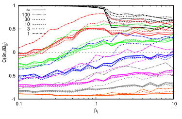
Figure 5: Theoretical prediction of $C(\delta n,\delta B_{\parallel})$ using synthetic spacecraft data as a function of ion plasma beta $\beta_{i}$ and fast-to-total compressible wave power $\mathcal{F}$ when the Taylor hypothesis is not assumed. Synthetic spacecraft data is produced using Vlasov-Maxwell eigenfunctions with 90% Alfvén wave power, and the remaining wave power split between fast and slow waves. Variation of the ratio of the probe to Alfvén velocity tests the sensitivity of the results to the Taylor hypothesis, where we have tested values $v/v_{A}=\infty,100,30,10,3,1$, where $v/v_{A}=\infty$ corresponds to the Taylor hypothesis.

5 Comparison to Observational Results and Discussion

Observational constraints suggest that turbulent magnetic power in inertial range turbulence in the solar wind consists of approximately 90% Alfvén waves, and the remaining 10% of the power in some mixture of the compressible kinetic fast and slow waves (Tu & Marsch, 1995; Bruno & Carbone, 2005). Numerical simulations of compressible MHD turbulence suggest that the distribution of turbulent power in wavevector space is isotropic for the fast waves and critically balanced for the Alfvén and slow waves (Cho & Lazarian, 2003). Therefore, we believe the most realistic model of solar wind turbulence using synthetic spacecraft data is given by the lower right-hand plot in Figure 4.

The analysis of the density-parallel magnetic field correlation using 10 years of Wind spacecraft data is discussed in detail in a companion work (Howes et al., 2012), so we give here only a few brief details. The density-parallel magnetic field correlation $C(\delta n,\delta B_{\parallel})$ is computed using measurements from the Magnetic Field Investigation (MFI) (Lepping, 1995) and the Three Dimensional Plasma (3DP) experiment (Lin, 1995) on the Wind spacecraft in the unperturbed solar wind at 1 AU during the years 1994-2004. Using 300-s intervals of ambient solar wind data (corresponding to inertial range scales of approximately $k\rho_{i}\in(5\times 10^{-3},5\times 10^{-2})$), the proton density and magnetic field measurements at 3 s cadence are decimated by a factor of 10 (to 30 s cadence). Magnetic field measurements are rotated to a field-aligned coordinate system, defined by the local mean field direction computed using 100-s windows, to compute $\delta B_{\parallel}$, and proton density data $\delta n=n-n_{0}$ is detrended over the same time intervals. The zero-lag cross-correlation $C(\delta n,\delta B_{\parallel})$ is computed for 119,512 data intervals. A joint histogram of $C(\delta n,\delta B_{\parallel})$ normalized in each $\beta_{i}$ bin is generated, and the peak histogram values and FWHM error bars are plotted on top of the theoretical synthetic spacecraft data plots of $C(\delta n,\delta B_{\parallel})$ from MHD (left) and kinetic (right) theory in Figure 6.

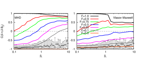
Figure 6: Comparison of measured values of the $C(\delta n,\delta B_{\parallel})$ cross-correlation (black dots with FWHM error bars) to the synthetic data predictions for MHD (left) and kinetic (right) theory given the ratio of fast wave to total compressible energy $\mathcal{F}$. Best agreement is with the kinetic theory for $\mathcal{F}=0.00$, indicating that the compressible component of solar wind turbulence is almost entirely in the kinetic slow mode. The compressive behavior is not well described by MHD for any $\mathcal{F}$.

For this direct comparison to the data, the theoretical results from the synthetic spacecraft data are computed in the same manner as the spacecraft measurements. In particular, the synthetic plasma volume is sampled at only $N=10$ uniformly spaced points along a trajectory of length $L=vT=\frac{10\pi}{24}\times 10^{2}\rho_{i}$, which corresponds to a range of scales $k\rho_{i}\in(4.8\times 10^{-3},4.8\times 10^{-2})$. The smaller number of timesteps and shorter total sampled length leads to a larger standard deviation using 256 ensembles than the Vlasov-Maxwell results in §4 and to slight quantitative changes in the $C(\delta n,\delta B_{\parallel})$ curves.

The agreement between the $C(\delta n,\delta B_{\parallel})$ from Wind spacecraft data and synthetic data curve for $\mathcal{F}=0$ in Figure 6 is striking, indicating that the observed correlation is consistent with a statistically negligible kinetic fast wave energy contribution for the large sample used in this study (Howes et al., 2012). We do note that a very small fraction of the intervals have $C(\delta n,\delta B_{\parallel})>0$, possibly indicating a minority population of fast waves. As discussed in our companion paper (Howes et al., 2012), this result has important consequences for the turbulent cascade of energy from large to small scales: since only the fast wave turbulent cascade is expected to nonlinearly transfer energy to whistler waves at $k\rho_{i}\gtrsim 1$, and the frequency mismatch between the fast and either the Alfvén or slow waves should prevent non-linear coupling, our analysis suggests that there is little or no transfer of large scale turbulent energy through the inertial range down to whistler waves at small scales.

Comparison of the observationally measured $C(\delta n,\delta B_{\parallel})$ in Figure 6 with both the MHD and kinetic results leads to another important conclusion of this study: the nature of the compressible fluctuations in the solar wind inertial range is not well modeled by MHD theory. This result is not surprising given that the solar wind is weakly collisional at inertial range scales, so a kinetic description is necessary to model accurately the compressible fluctuations.

Our study also enables us to constrain the wavevector distribution of slow wave energy by comparing the observational results with the three plots in the bottom row of Figure 4. The leftmost plot has an isotropic distribution of slow wave power and shows two features in the $\mathcal{F}=0$ curve not seen in the observed data: (1) a bump at $\beta_{i}\sim 1$ and (2) a slight increase in the correlation value at $\beta_{i}\lesssim 0.3$. These quantitative changes in the $\mathcal{F}=0$ curve appear the same with or without the Alfvén waves at $\beta_{i}\lesssim 1$ (compare the left plots in the third and fourth row of Figure 4), so this effect is not due to the isotropic distribution of Alfvén waves. Therefore, the slow waves appear to be anisotropically distributed, and may be well described by critical balance as suggested by theories of slow wave passive advection (Maron & Goldreich, 2001; Schekochihin et al., 2009). However, the uncertainty of the Wind measurements cannot definitively rule out the possibility of an isotropic distribution for the slow mode.

One of the key points of our companion work (Howes et al., 2012) is the interpretation that the compressible fluctuations in the solar wind consist of a critically balanced distribution of kinetic slow wave fluctuations. Previous analyses have generally dismissed the possibility of kinetic slow waves because, in an isotropic Maxwellian plasma with warm ions, the collisionless damping via free-streaming along the magnetic field is strong (Barnes, 1966). However, the damping rate of the slow waves for the nearly perpendicular wavevectors of a critically balanced distribution is proportional to the parallel component of the wavevector, $\gamma\propto k_{\parallel}$. This feature can be seen in the right column of Figure 1, where the slow wave damping rate (blue) is zero at perpendicular wavevectors $\theta=90^{\circ}$ (open circles) and increases as the wavevector angle decreases. For exactly perpendicular wavevectors, the damping rate drops to zero—this perpendicular limit of the slow wave corresponds to an undamped, non-propagating pressure-balanced structure (PBS). It has been derived theoretically by Schekochihin et al. (2009) and demonstrated numerically by Maron & Goldreich (2001) that the Alfvén wave dynamics advects and cascades the slow waves, so the energy cascade rate of the slow waves is related not to the slow wave frequency, but to the Alfvén wave frequency. Therefore, although the slow wave fluctuations at the high $k_{\parallel}$ boundary of critical balanced distribution (along $k_{\parallel}\sim k_{0}^{1/3}k_{\perp}^{2/3}$) may suffer strong collisionless damping, the more nearly perpendicular slow waves may be cascaded to smaller scales on the timescale of the Alfvénic turbulence, while the collisionless damping of these modes remains weak. This could lead to a slow wave energy distribution that is more anisotropic than critical balance, possibly with $k_{\parallel}\ll k_{0}^{1/3}k_{\perp}^{2/3}$.

Using synthetic spacecraft data, we can test whether this picture of a distribution of slow wave power that is more anisotropic than critical balance is consistent with the observational findings in Figure 6. To do this, we repeat the analysis in the lower right plot of Figure 4 but with a more anisotropic distribution of slow waves given by $k_{\parallel}\leq k_{0}^{2/3}k_{\perp}^{1/3}$. The results of this test, shown in Figure 7, demonstrate that the $\mathcal{F}=0$ curve does not change significantly for a more anisotropic slow wave distribution. Therefore, the picture of the solar wind compressible fluctuations comprised of slow wave fluctuations that are more anisotropically distributed than critical balance is consistent with the observational data.

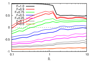
Figure 7: Comparison of synthetic data predictions for $C(\delta n,\delta B_{\parallel})$ with isotropic fast mode power, critically balanced Alfvén mode power, and either critically balanced (solid) or more anisotropic than critical balance (dashed) slow mode power. For the more anisotropic than critical balance distribution, all modes with $k_{\parallel}>k_{0}^{2/3}k_{\perp}^{1/3}$ are set to zero, where $k_{0}$ is the minimum wavenumber of the wavenumber domain. The difference between the lines is attributable to our choice for specifying the fraction of wave power individually for each Fourier component: the more anisotropic distribution contains less total slow wave power. The lines for the $\mathcal{F}=0$ are nearly identical for both power distributions, signifying that $C(\delta n,\delta B_{\parallel})$ can not be used to differentiate between critical balance and more anisotropic distributions.

One of the limitations of this investigation is that the Vlasov-Maxwell eigenfunctions are computed assuming isotropic Maxellian equilibrium distributions. Plasma measurements in the solar wind frequently find anisotropic temperature distributions and non-Maxwellian tails at high energy (Marsch, 1991, 2006). In particular, it is possible that mirror modes may contribute to the measured anti-correlation between the density and parallel magnetic field, although an analysis of 10 years of Wind data show that only a small fraction of the solar wind measurements occupy the region of parameter space near the mirror instability threshold (Bale et al., 2009). How the density-parallel magnetic field correlation is altered by these conditions is an important issue to be addressed in future work.

6 Conclusion

In this paper, we have presented the first application of kinetic plasma theory to analyze and interpret the compressible fluctuations in the inertial range of solar wind turbulence. This novel approach is motivated by the fact that the dynamics in the solar wind plasma is weakly collisional, a limit in which MHD theory, used in all previous related investigations, is formally invalid. Investigation of the compressible fast and slow wave modes requires a kinetic description to resolve both the wave dynamics and the collisionless kinetic damping mechanisms.

We identify quantitatively the linear kinetic wave modes of Vlasov-Maxwell theory that correspond to the linear MHD fast and slow wave modes, and verify that the general qualitative properties of the density-parallel magnetic field correlation $C(\delta n,\delta B_{\parallel})$—that fast waves are positively correlated, and slow waves are negatively correlated—remain unchanged for the weakly collisional conditions of the solar wind plasma.

We then describe the procedure used to generate synthetic spacecraft data used to interpret actual single-point spacecraft measurements of turbulence in the solar wind. We define and discuss the quasi-linear premise—that some properties of magnetized plasma turbulence can be understood by modeling the turbulence as a collection of randomly phased, linear waves—upon which the method of synthetic spacecraft data is based. Theoretical arguments for the validity of the quasi-linear premise are presented; a review of supporting and conflicting evidence for the quasi-linear premise in the literature is presented in Howes et al. (2011). We outline how the synthetic plasma data cubes are used to generate synthetic reduced time series of single-point measurements that can be analyzed using the same procedures as the actual spacecraft measurements. Comparison of the results of the analyses of both the synthetic and actual spacecraft data enables novel physical interpretations of the solar wind turbulence measurements (Howes et al., 2012).

Next, we use the synthetic spacecraft data method to predict the characteristics of the density-parallel magnetic field correlation $C(\delta n,\delta B_{\parallel})$ as a function of plasma $\beta_{i}$ in the presence of a turbulent spectrum of wave modes. Comparison of these synthetic predictions of $C(\delta n,\delta B_{\parallel})$, based on both linear MHD and linear Vlasov-Maxwell eigenfunctions, to the results from an analysis of a 10-year data set of observations from the Wind spacecraft leads to the following conclusions:

1. The predicted $C(\delta n,\delta B_{\parallel})$ and its dependence on plasma $\beta_{i}$ using linear MHD eigenfunctions is significantly different from the prediction using linear Vlasov-Maxwell eigenfunctions. Only the prediction based on kinetic theory appears to agree with the spacecraft measurements, leading to the expected conclusion that MHD theory is inadequate to describe the compressible fluctuations in the weakly collisional solar wind.

2. Strong a posteriori evidence for the validity of the quasi-linear premise is provided by the striking agreement between the observationally determined $C(\delta n,\delta B_{\parallel})$ over a very large statistical sample and the predicted $C(\delta n,\delta B_{\parallel})$ based on synthetic spacecraft data.

3. The observed $C(\delta n,\delta B_{\parallel})$ computed in a companion work (Howes et al., 2012) is consistent with a statistically negligible kinetic fast wave energy contribution for the large sample used in this study. Note, however, that the our companion work also found that a very small fraction of the intervals have $C(\delta n,\delta B_{\parallel})>0$, possibly indicating a trace population of fast waves (Howes et al., 2012).

4. The quantitative dependence of $C(\delta n,\delta B_{\parallel})$ on the ion plasma beta $\beta_{i}$ provides evidence that the slow wave fluctuations are not isotropically distributed, but rather have an anisotropic distribution, that is possibly given by the condition of critical balance (Goldreich & Sridhar, 1995) or that is more anisotropic than critical balance.

In conclusion, our analysis using kinetic theory to interpret the compressible fluctuations motivates the following physical model of the turbulent fluctuations in the solar wind inertial range. In this model, the solar wind inertial range consists of a mixture of turbulent fluctuations, with 90% of the energy due to incompressible Alfvénic fluctuations and the remaining 10% of the energy due to compressible slow wave fluctuations. The Alfvénic turbulent power is distributed anisotropically in wave vector space according to critical balance. The turbulent Alfvén wave dynamics advects and cascades the slow wave fluctuations to smaller scales at the Alfvén wave frequency. The slow wave turbulent power may be either critically balanced, or more anisotropic than critical balance due to collisionless damping of the slow wave fluctuations.

Since only the fast wave turbulent cascade is expected to nonlinearly transfer energy to whistler waves at $k\rho_{i}\gtrsim 1$, and the frequency mismatch between the fast and either the Alfvén or slow waves should prevent non-linear coupling, there is little or no transfer of large scale turbulent energy through the inertial range down to whistler waves at small scales. Therefore, any whistler wave fluctuations at scales $k\rho_{i}\gtrsim 1$ must be generated by some other process, e.g., kinetic temperature anisotropy instabilities (Kasper et al., 2002; Hellinger et al., 2006; Bale et al., 2009) or kinetic drift instabilities driven by differential flow between protons and alpha particles (McKenzie et al., 1993; Kasper et al., 2008; Bourouaine et al., 2011).

Finally, the lack of statistically significant fast wave energy has important implications for efficient numerical modeling of solar wind turbulent fluctuations. This work demonstrates clearly the importance of a kinetic approach to model adequately the turbulent fluctuations, yet a general kinetic numerical treatment—e.g., the Particle-In-Cell (PIC) method—in three spatial dimensions (required for physically relevant modeling of the dominant nonlinear interactions in solar wind turbulence (Howes et al., 2011)) is too computationally costly to be presently feasible. Fortunately, it is possible to perform kinetic numerical simulations of solar wind turbulence in three spatial dimensions using gyrokinetics, a rigorous, low-frequency, anisotropic limit of kinetic theory (Rutherford & Frieman, 1968; Frieman & Chen, 1982; Howes et al., 2006; Schekochihin et al., 2009). In the derivation of the gyrokinetic equation, the crucial step is an averaging over the particle gyrophase, which leads to a theory with the following properties: the fast/whistler wave and the cyclotron resonances are discarded; all finite Larmor radius effects and collisionless dissipation via the Landau resonance are retained; and one of the dimensions of velocity in phase space is eliminated, reducing the particle distribution function from six to five dimensions. It has been previously pointed out that one cannot rule out the contribution of fast wave or whistler wave physics to solar wind turbulence, and that that therefore gyrokinetics is an incomplete description of the turbulence (Matthaeus et al., 2008). The novel observational analysis presented here suggests that the fast wave, in fact, does not play a statistically significant role in the turbulent dynamics of the inertial range, and that therefore a gyrokinetic approach sufficiently describes all important physical mechanisms in the solar wind inertial range.

Appendix A Normalized MHD Linear Eigenfunctions

The ideal, compressible MHD equations are given by the continuity equation,

$$\frac{\partial\rho}{\partial t}+\textbf{U}\cdot\nabla\rho=-\rho\nabla\cdot\textbf{U},$$ (A1)

the momentum equation,

$$\rho\left(\frac{\partial\textbf{U}}{\partial t}+\textbf{U}\cdot\nabla\textbf{U}\right)=-\nabla\left(p+\frac{B^{2}}{8\pi}\right)+\frac{(\textbf{B}\cdot\nabla)\textbf{B}}{4\pi},$$ (A2)

the induction equation,

$$\frac{\partial\textbf{B}}{\partial t}=\nabla\times(\textbf{U}\times\textbf{B}),$$ (A3)

and an adiabatic equation of state,

$$\frac{\partial p}{\partial t}+\textbf{U}\cdot\nabla p=-\gamma p\nabla\cdot\textbf{U}.$$ (A4)

Here the MHD fluid is completely described by its mass density $\rho=n(m_{i}+m_{e})$, fluid velocity $\mathbf{U}$, magnetic field $\mathbf{B}$, and scalar thermal pressure $p$. The adiabatic index for a proton and electron plasma is $\gamma=5/3$. This system of equations can be derived rigorously from plasma kinetic theory in the MHD limit of strong collisionality $\nu\gg\omega$, large scales compared to the ion Larmor radius $k\rho_{i}\ll 1$, and non-relativistic conditions (Kulsrud, 1983).

Although the weakly collisional conditions of the solar wind plasma violate the strong collisionality formally required for the validity of MHD, this system has nevertheless been widely used to study the turbulent dynamics of the solar wind inertial range. That this simplified approach has not met with widespread failure is likely due to the fact that the turbulent dynamics in the inertial range is dominated by Alfvénic motions (Belcher & Davis, 1971; Tu & Marsch, 1995; Bruno & Carbone, 2005). Alfvénic fluctuations at inertial range scales are incompressible, and it has been shown that for anisotropic fluctuations with $k_{\parallel}\ll k_{\perp}$ (the anisotropy generally observed in the magnetized plasma turbulence (Robinson & Rusbridge, 1971; Zweben et al., 1979; Montgomery & Turner, 1981; Sahraoui et al., 2010; Chen et al., 2011)), the dynamics of Alfvénic fluctuations are rigorously described by the equations of reduced MHD, even under weakly collisional conditions (Schekochihin et al., 2009). The compressible fast and slow wave fluctuations, on the other hand, are substantially modified in weakly collisional conditions, so their dynamics must be treated using kinetic theory (Kulsrud, 1983; Schekochihin et al., 2009), as has been demonstrated in the investigation presented here.

In this appendix, we derive the compressible MHD linear dispersion relation and eigenfunctions in dimensionless units constructed specifically for our study of compressible solar wind fluctutations. Without loss of generality, we specify a wavevector $\mathbf{k}=k_{\perp}\mbox{$\hat{\mathbf{x}}$}+k_{\parallel}\mbox{$\hat{\mathbf{z}}$}$ and an equilibrium magnetic field $\mathbf{B}_{0}=B_{0}\mbox{$\hat{\mathbf{z}}$}$. We separate mean from fluctuating quantities using $\rho=\rho_{0}+\delta\rho$, $\mathbf{U}=\delta\mathbf{U}$, $\mathbf{B}=\mathbf{B}_{0}+\delta\mathbf{B}$, and $p=p_{0}+\delta p$, where we specify that there is no mean fluid velocity. We then linearize equations (A1)–(A4) and Fourier transform the equations in both space and time. Next, we convert each of the variables to dimensionless units and define the dimensionless frequency and other parameters as follows:

$$\begin{array}[]{ccccccccc}\overline{\delta n}&=&\overline{\delta\rho}&=&\delta\rho/\rho_{0}&\mbox{\hskip 72.26999pt}&\overline{\omega}&=&\omega/(kv_{A})\\ &&\overline{\delta\mathbf{U}}&=&\delta\mathbf{U}/v_{A}&\mbox{\hskip 72.26999pt}&\beta&=&c_{s}^{2}/v_{A}^{2}\\ &&\overline{\delta\mathbf{B}}&=&\delta\mathbf{B}/B_{0}&\mbox{\hskip 72.26999pt}&c_{s}^{2}&=&\gamma p_{0}/\rho_{0}\\ &&\overline{\delta p}&=&\delta p/p_{0}&\mbox{\hskip 72.26999pt}&v_{A}^{2}&=&B_{0}^{2}/4\pi\rho_{0}\\ \end{array}$$ (A5)

In this normalization, the linear dispersion relation takes the form

$$\left(\overline{\omega}^{2}-\cos^{2}\theta\right)\left[\overline{\omega}^{4}-\overline{\omega}^{2}(1+\beta)+\beta\cos^{2}\theta\right]=0$$ (A6)

where the first factor in parentheses corresponds to the two Alfvén wave solutions, and the second factor in the brackets corresponds to the two slow and two fast wave solutions. This demonstrates the important property that the normalized compressible MHD linear dispersion relation depends on only two parameters, $\omega/(kv_{A})=\overline{\omega}_{MHD}(\beta,\theta)$: the plasma beta $\beta$ and the angle $\theta$ between the local mean magnetic field $\mathbf{B}_{0}$ and the direction of the wavevector $\mathbf{k}$.

The linear Alfvén wave solutions have frequency

$$\overline{\omega}^{2}=\cos^{2}\theta$$ (A7)

and eigenfunctions specified in terms of $\overline{\delta U_{y}}$ given by

$$\overline{\delta B_{y}}=\pm\overline{\delta U_{y}}$$ (A8)

$$\overline{\delta n}=\overline{\delta U_{x}}=\overline{\delta U_{\parallel}}=\overline{\delta B_{x}}=\overline{\delta B_{\parallel}}=\overline{\delta p}=0$$ (A9)

The linear slow and fast wave solutions have frequency

$$\overline{\omega}^{2}=\frac{1+\beta\pm\sqrt{(1+\beta)^{2}-4\beta\cos^{2}\theta}}{2},$$ (A10)

where the plus sign corresponds to the fast wave, and the minus sign to the slow wave. The eigenfunctions, specified in terms of $\overline{\delta B_{\parallel}}$, are given by

$$\overline{\delta n}=\frac{-\overline{\delta B_{\parallel}}\overline{\omega}^{2}}{\overline{\omega}^{2}-\beta\cos^{2}\theta}$$ (A11)

$$\overline{\delta B_{x}}=-\overline{\delta B_{\parallel}}\cot\theta$$ (A12)

$$\overline{\delta U_{x}}=\overline{\omega}\overline{\delta B_{\parallel}}\csc\theta$$ (A13)

$$\overline{\delta U_{\parallel}}=\frac{\overline{\omega}\beta\cos\theta}{\overline{\omega}^{2}-\beta\cos^{2}\theta}\overline{\delta B_{\parallel}}$$ (A14)

$$\overline{\delta U_{y}}=\overline{\delta B_{y}}=0$$ (A15)

Since the synthetic data sets are created by specifying a spectrum of fluctuations over some range of angles, the statistical correlations of the fluctuations depend on only three factors: (a) angular power distribution, (b) wave mode fraction, and (c) plasma $\beta$.

Appendix B Determining Kinetic Counterparts of Slow vs. Fast MHD Waves

The kinetic fast and slow modes are both part of the double-valued magnetosonic solution (Krauss-Varban et al., 1994) and are separated by a branch cut from $\theta\approx 30^{\circ}$ to $0^{\circ}$ at $\beta_{i}\approx 1.3$. This branch cut is similar to the magnetic and acoustic transition for the MHD fast and slow modes at $\beta=1$ for near parallel wavevectors. The kinetic fast and slow modes behave in an analogous fashion: the near parallel kinetic fast mode has the same phase velocity as the Alfvén mode for $\beta_{i}<1.3$; and the near parallel kinetic slow mode matches the Alfvén mode for $\beta_{i}>1.3$ (see the center column of Figure 1). In this work, we label wave modes using a scheme that identifies the modes at $\theta=90^{\circ}$, where there is no ambiguity in identification, and then follows the linear dispersion relation as $\theta$ is decreased to zero.

The compressible inertial range linear wave modes with near parallel wavevectors can be characterized as being either magnetic or acoustic. The magnetic modes have phase velocities similar to the Alfvén wave, while the acoustic modes are more heavily damped than either the Alfvén or the magnetic modes. From this point of view, the fast mode is the magnetic mode and the slow mode is the acoustic mode for $\beta_{i}<1.3$, while the converse is true for $\beta_{i}>1.3$. Interestingly, for $\beta_{i}<1.3$, the magnetic (fast) mode has $C(\delta n,\delta B_{\parallel})\simeq 1$ and the acoustic (slow) mode has $C(\delta n,\delta B_{\parallel})\simeq-1$; but, for $\beta_{i}>1.3$, both modes have $C(\delta n,\delta B_{\parallel})\simeq 0$ (see Figure 2). It is this transition that is responsible for some of the qualitative features in the lower two rows of Figure 4. In particular, the abrupt jump on the $\mathcal{F}=1$ curve (black) at $\beta_{i}\sim 1.3$ in the left and right columns (where fast waves are isotropically distributed and so include this region of wavevector space) and in the $\mathcal{F}=0$ curve (orange) at $\beta_{i}\sim 1.3$ in the left column (where the slow waves are isotropically distributed) are due to this transition.

This identification of modes has important physical ramifications, especially at scales near the transition to the dissipation range. As length scales decrease towards the ion inertial length, it is the magnetic mode, and not strictly the kinetic fast mode, that transitions to the parallel whistler wave. However, the results presented in this paper suggest a lack of parallel slow wave energy as well as statistically negligible fast wave energy in the solar wind inertial range, so the difficulties of mode identification in this region of parameter space may not be problematic for studies of solar wind turbulence.

References

- Bale et al. (2009) Bale, S. D., Kasper, J. C., Howes, G. G., Quataert, E., Salem, C., & Sundkvist, D. 2009, Phys. Rev. Lett., 103, 211101
- Barnes (1966) Barnes, A. 1966, Phys. Fluids, 9, 1483
- Baumjohann & Treumann (1996) Baumjohann, W., & Treumann, R. A. 1996, Basic space plasma physics (London: Imperial College Press)
- Bavassano et al. (2004) Bavassano, B., Pietropaolo, E., & Bruno, R. 2004, Annales Geophysicae, 22, 689
- Belcher & Davis (1971) Belcher, J. W., & Davis, L. 1971, J. Geophys. Res., 76, 3534
- Boldyrev (2006) Boldyrev, S. 2006, Phys. Rev. Lett., 96, 115002
- Bourouaine et al. (2011) Bourouaine, S., Marsch, E., & Neubauer, F. M. 2011, Astrophys. J. Lett., 728, L3+
- Bruno & Carbone (2005) Bruno, R., & Carbone, V. 2005, Living Reviews in Solar Physics, 2, 4
- Burlaga (1968) Burlaga, L. F. 1968, Sol. Phys., 4, 67
- Burlaga & Ogilvie (1970) Burlaga, L. F., & Ogilvie, K. W. 1970, Sol. Phys., 15, 61
- Burlaga et al. (1990) Burlaga, L. F., Scudder, J. D., Klein, L. W., & Isenberg, P. A. 1990, J. Geophys. Res., 95, 2229
- Chen et al. (2011) Chen, C. H. K., Mallet, A., Yousef, T. A., Schekochihin, A. A., & Horbury, T. S. 2011, Mon. Not. Roy. Astron. Soc., 415, 3219
- Cho & Lazarian (2003) Cho, J., & Lazarian, A. 2003, Mon. Not. Roy. Astron. Soc., 345, 325
- Cho & Vishniac (2000) Cho, J., & Vishniac, E. T. 2000, Astrophys. J., 539, 273
- Coleman (1968) Coleman, Jr., P. J. 1968, Astrophys. J., 153, 371
- Dmitruk & Matthaeus (2009) Dmitruk, P., & Matthaeus, W. H. 2009, Phys. Plasmas, 16, 062304
- Elsasser (1950) Elsasser, W. M. 1950, Physical Review, 79, 183
- Forman et al. (2011) Forman, M. A., Wicks, R. T., & Horbury, T. S. 2011, Astrophys. J., 733, 76
- Frieman & Chen (1982) Frieman, E. A., & Chen, L. 1982, Phys. Fluids, 25, 502
- Galtier et al. (2000) Galtier, S., Nazarenko, S. V., Newell, A. C., & Pouquet, A. 2000, J. Plasma Phys., 63, 447
- Goldreich & Sridhar (1995) Goldreich, P., & Sridhar, S. 1995, Astrophys. J., 438, 763
- Goldreich & Sridhar (1997) —. 1997, Astrophys. J., 485, 680
- Hellinger et al. (2006) Hellinger, P., Trávníček, P., Kasper, J. C., & Lazarus, A. J. 2006, Geophys. Res. Lett., 33, 9101
- Higdon (1984) Higdon, J. C. 1984, Astrophys. J., 285, 109
- Horbury et al. (2008) Horbury, T. S., Forman, M., & Oughton, S. 2008, Phys. Rev. Lett., 101, 175005
- Howes (2009) Howes, G. G. 2009, Nonlin. Proc. Geophys., 16, 219
- Howes et al. (2012) Howes, G. G., Bale, S. D., Klein, K. G., Chen, C. H. K.and Salem, C. S., & TenBarge, J. M. 2012, Astrophys. J. Lett., submitted
- Howes et al. (2006) Howes, G. G., Cowley, S. C., Dorland, W., Hammett, G. W., Quataert, E., & Schekochihin, A. A. 2006, Astrophys. J., 651, 590
- Howes et al. (2008a) —. 2008a, J. Geophys. Res., 113, A05103
- Howes et al. (2008b) Howes, G. G., Dorland, W., Cowley, S. C., Hammett, G. W., Quataert, E., Schekochihin, A. A., & Tatsuno, T. 2008b, Phys. Rev. Lett., 100, 065004
- Howes et al. (2011) Howes, G. G., Tenbarge, J. M., & Dorland, W. 2011, Phys. Plasmas, 18, 102305
- Howes et al. (2011) Howes, G. G., TenBarge, J. M., Dorland, W., Quataert, E., Schekochihin, A. A., Numata, R., & Tatsuno, T. 2011, Phys. Rev. Lett., 107, 035004
- Howes et al. (2011) Howes, G. G., TenBarge, J. M., & Klein, K. G. 2011, Astrophys. J., in preparation
- Hunana et al. (2011) Hunana, P., Laveder, D., Passot, T., Sulem, P. L., & Borgogno, D. 2011, Astrophys. J., 743, 128
- Kasper et al. (2002) Kasper, J. C., Lazarus, A. J., & Gary, S. P. 2002, Geophys. Res. Lett., 29, 20
- Kasper et al. (2008) —. 2008, Phys. Rev. Lett., 101, 261103
- Kellogg & Horbury (2005) Kellogg, P. J., & Horbury, T. S. 2005, Ann. Geophys., 23, 3765
- Krauss-Varban et al. (1994) Krauss-Varban, D., Omidi, N., & Quest, K. B. 1994, J. Geophys. Res., 99, 5987
- Kulsrud (1983) Kulsrud, R. M. 1983, in Handbook of Plasma Physics, Vol. 1, Basic Plasma Physics I, ed. A. A. Galeev & R. N. Sudan (North Holland), 115–145
- Lepping (1995) Lepping, R. 1995, Space Sci Rev, 71, 207
- Lin (1995) Lin, R. P. 1995, Space Sci Rev, 71, 125
- Lithwick & Goldreich (2003) Lithwick, Y., & Goldreich, P. 2003, Astrophys. J., 582, 1220
- Luo & Wu (2010) Luo, Q. Y., & Wu, D. J. 2010, Astrophys. J. Lett., 714, L138
- Maron & Goldreich (2001) Maron, J., & Goldreich, P. 2001, Astrophys. J., 554, 1175
- Marsch (1991) Marsch, E. 1991, in Physics of the Inner Heliosphere II. Particles, Waves and Turbulence., ed. E. Schwenn, R. andMarsch (Berlin: Springer-Verlag), 45–133
- Marsch (2006) Marsch, E. 2006, Living Rev. Solar Phys., 3
- Matthaeus et al. (1991) Matthaeus, W. H., Klein, L. W., Ghosh, S., & Brown, M. R. 1991, J. Geophys. Res., 96, 5421
- Matthaeus et al. (2008) Matthaeus, W. H., Servidio, S., & Dmitruk, P. 2008, Phys. Rev. Lett., 101, 149501
- McComas et al. (1995) McComas, D. J., Barraclough, B. L., Gosling, J. T., Hammond, C. M., Phillips, J. L., Neugebauer, M., Balogh, A., & Forsyth, R. J. 1995, J. Geophys. Res., 100, 19893
- McKenzie et al. (1993) McKenzie, J. F., Marsch, E., Baumgaertel, K., & Sauer, K. 1993, Ann. Geophys., 11, 341
- Montgomery et al. (1987) Montgomery, D., Brown, M. R., & Matthaeus, W. H. 1987, J. Geophys. Res., 92, 282
- Montgomery & Matthaeus (1995) Montgomery, D., & Matthaeus, W. H. 1995, Astrophys. J., 447, 706
- Montgomery & Turner (1981) Montgomery, D., & Turner, L. 1981, Phys. Fluids, 24, 825
- Narita et al. (2011) Narita, Y., Gary, S. P., Saito, S., Glassmeier, K.-H., & Motschmann, U. 2011, Geophys. Res. Lett., 38, L05101
- Ng & Bhattacharjee (1996) Ng, C. S., & Bhattacharjee, A. 1996, Astrophys. J., 465, 845
- Ng & Bhattacharjee (1997) —. 1997, Phys. Plasmas, 4, 605
- Parashar et al. (2010) Parashar, T. N., Servidio, S., Breech, B., Shay, M. A., & Matthaeus, W. H. 2010, Phys. Plasmas, 17, 102304
- Podesta (2009) Podesta, J. J. 2009, Astrophys. J., 698, 986
- Quataert (1998) Quataert, E. 1998, Astrophys. J., 500, 978
- Reisenfeld et al. (1999) Reisenfeld, D. B., McComas, D. J., & Steinberg, J. T. 1999, Geophys. Res. Lett., 26, 1805
- Roberts (1990) Roberts, D. A. 1990, J. Geophys. Res., 95, 1087
- Roberts et al. (1987a) Roberts, D. A., Goldstein, M. L., Klein, L. W., & Matthaeus, W. H. 1987a, J. Geophys. Res., 92, 12023
- Roberts et al. (1987b) —. 1987b, J. Geophys. Res., 92, 11021
- Robinson & Rusbridge (1971) Robinson, D. C., & Rusbridge, M. G. 1971, Phys. Fluids, 14, 2499
- Rutherford & Frieman (1968) Rutherford, P. H., & Frieman, E. A. 1968, Phys. Fluids, 11, 569
- Sahraoui et al. (2010) Sahraoui, F., Goldstein, M. L., Belmont, G., Canu, P., & Rezeau, L. 2010, Phys. Rev. Lett., 105, 131101
- Schekochihin et al. (2009) Schekochihin, A. A., Cowley, S. C., Dorland, W., Hammett, G. W., Howes, G. G., Quataert, E., & Tatsuno, T. 2009, Astrophys. J. Supp., 182, 310
- Shebalin et al. (1983) Shebalin, J. V., Matthaeus, W. H., & Montgomery, D. 1983, J. Plasma Phys., 29, 525
- Sridhar & Goldreich (1994) Sridhar, S., & Goldreich, P. 1994, Astrophys. J., 433, 612
- Stix (1992) Stix, T. H. 1992, Waves in Plasmas (New York: American Institute of Physics)
- Taylor (1938) Taylor, G. I. 1938, Proc. Roy. Soc. A, 164, 476
- Tu & Marsch (1994) Tu, C.-Y., & Marsch, E. 1994, J. Geophys. Res., 99, 21481
- Tu & Marsch (1995) —. 1995, Space Sci. Rev., 73, 1
- Vellante & Lazarus (1987) Vellante, M., & Lazarus, A. J. 1987, J. Geophys. Res., 92, 9893
- Wicks et al. (2010) Wicks, R. T., Horbury, T. S., Chen, C. H. K., & Schekochihin, A. A. 2010, Mon. Not. Roy. Astron. Soc., 407, L31
- Yao et al. (2011) Yao, S., He, J.-S., Marsch, E., Tu, C.-Y., Pedersen, A., Rème, H., & Trotignon, J. G. 2011, Astrophys. J., 728, 146
- Zweben et al. (1979) Zweben, S. J., Menyuk, C. R., & Taylor, R. J. 1979, Phys. Rev. Lett., 42, 1270