Higher Order Methods for Differential Inclusions

1 Introduction

In this paper, we compute reachable sets of differential inclusions,

$$\dot{x}(t)\in F(x(t)),\,\,x(0)=x_{0},$$ (1)

where $F$ is a continuous set-valued map with compact and convex values. A solution of the differential inclusion (1) is an absolutely continuous function $x:[0,T]\rightarrow\mathbb{R}^{n}$, such that for almost all $t\in[0,T]$, $x(\cdot)$ is differentiable at $t$ and $\dot{x}(t)\in F(x(t))$. The solution set $S_{T}(x_{0})\subset C([0,T],\mathbb{R}^{n})$ is defined as

$$S_{T}(x_{0})=\{x(\cdot)\in C([0,T],\mathbb{R}^{n})\,\mid\,x(\cdot)\text{ is a solution of }\dot{x}(t)\in F(x(t))\text{ with }x(0)=x_{0}\}.$$

The reachable set at time $t$, $R(x_{0},t)\subset\mathbb{R}^{n}$, is defined as

$$R(x_{0},t)=\{x(t)\in\mathbb{R}^{n}\,|x(\cdot)\in S_{t}(x_{0})\}.$$

In particular, we are interested in higher-order method for computation of a rigorous over-approximation of the reachable set of a differential inclusion.

Differential inclusions are generalization of differential equations having multivalued right-hand sides, see [2], [8], [25]. They give a mathematical setting for studying differential equations with discontinuous right-hand sides. In fact, taking a closed, convex hull of the right-hand side, one obtains a differential inclusion. Solutions of this differential inclusion are known as Fillipov solutions of the original differential equation; see [12].

One important application area for differential inclusions is control theory. Suppose we are given an interval $[0,T]$, and absolutely continuous function $x(\cdot)$ which satisfies the inclusion (1), where $F(x)=f(x,U)=\bigcup_{u\in U}f(x(t),u)$ for almost all $t\in[0,T]$. It is known that if the set $U$ is compact and separable, $f$ is continuous, and $f(x,U)$ is convex for all $x$, then there exists a bounded measurable function $u(t)\in U$, known as admissible control input, such that $x(t)$ is the solution of the control system,

$$\dot{x}(t)=f(x(t),u(t)),\,\,\,x(0)=x_{0}.$$ (2)

The proof of the above is given in [2], and with slight changes in the assumptions, also in [22] or [18]. On the other hand, it is easy to see that each solution of a control system (2) for a given admissible control input is also a solution of a differential inclusion (1). Therefore, if a control system is not completely controllable one may want to compute reachable sets corresponding to all possible inputs ($u(t)\in U$) which is equivalent to computing a reachable set of a differential inclusion.

Similarly, we obtain a differential inclusion from a noisy system of differential equations

$$\dot{x}(t)=f(x(t),v(t)),\quad x(0)=x_{0},\quad v(t)\in V.$$ (3)

Although the form of (2) and (3) are identical, the interpretation is different; in (2), the input $u(t)$ can be chosen by the designer, whereas in (3), the input is determined by the environment.

Differential inclusions can also arise as reduced models of high-dimensional systems of differential equations. For example, suppose we have a large-scale system given in the form of differential equation $\dot{x}(t)=f(x(t))$. In general, it is very hard to analyse large-scale systems and most of the times performing model reduction is necessary. This gives a simplified model in the form of $\dot{z}(t)=h(z(t))+e(t)$, where $|e(t)|<\epsilon$ represents the error that occurred while simplifying the model.

For reliability purposes many engineering systems require availability of verification tools. In order to verify a system, we must guarantee that an approximate solution will contain the actual solution of the system. If there is uncertainty in the system, lack of controllability, or just a variety of available dynamics, one needs to use differential inclusion models. For verification purposes, one needs to compute over-approximations to the set of solutions.

An important tool in the study of input-affine control systems (2) is based on the Fliess expansion [13], in which the evolution over a time-step $h$ is expanded as a power-series in integrals of the input. A numerical method based on this approach was given in [15]. The method cannot be directly applied to study noisy systems (3), since for this problem we need to compute the evolution over all possible inputs, and this point is only briefly addressed.

The first result on the computation of the solution set of a differential inclusion was given in [23], who considered Lipschitz differential inclusions, and gave a polyhedral method for obtaining an approximation of the solution set $S(x_{0})$ to an arbitrary known accuracy. In the case where $F$ is only upper-semicontinuous with compact, convex values, it is possible to compute arbitrarily accurate over-approximations to the solution set, as shown in [5].

Some different techniques and various types of numerical methods have been proposed as approximations to the solution set of a differential inclusion. For example, ellipsoidal calculus was used in [20], a Lohner-type algorithm in [17], grid-based methods in [23] and [4], optimal control in [3] and discrete approximations in [9, 10, 11], [14]. However, these algorithms either do not give rigorous over-approximations, or are approximations of low-order (e.g. Euler approximations with a first-order single-step truncation error). Essentially, the only algorithms mentioned above that could give arbitrary accurate error estimates are the ones that use grids. However, higher order discretization of a state space greatly affects efficiency of the algorithm. It was noted in [4] that if one is trying to obtain higher order error estimates on the solution set of differential inclusions then grid methods should be avoided.

In order to provide an over-approximation of the reachable set of (1), we compute solutions of an “approximate” system

$$\dot{y}(t)=f(y(t),w_{k}(t)),\quad y(t_{k})=x(t_{k}),\ w_{k}(\cdot)\in W,$$

for $t\in[t_{k},t_{k+1}]$, and add the uniform error bound on the difference of the two solutions. We provide formulas for the local error based on Lipschitz constants and bounds on higher-order derivatives. The method is based on a Fliess-like expansion, and extends the results of [15] by providing error estimates which are valid for all possible inputs.

We can obtain improved estimates by the use of the logarithmic norm. The logarithmic norm was introduced independently in [7], and [19] in order to derive error estimates to initial value problems, see also [26]. Using the logarithmic norm is advantageous over the use of Lipschitz constant in the sense that the logarithmic norm can have negative values, and thus, one can distinguish between forward and reverse time integration, and between stable and unstable systems. The definition of the logarithmic norm and a theorem on the logarithmic norm estimate is given in Section 2.

The numerical result given in Section 6 were obtained using the function calculus implemented in the tool Ariadne [1] for reachability analysis and verification of hybrid systems. In particular, we use polynomial models for the rigorous approximation of continuous functions. Polynomial model expresses approximations to a function in the form of a polynomial (defined over a suitably small domain) plus an interval remainder, and are essentially the same as the Taylor models of [24].

The paper is organized as follows. In Section 2, we give key ingredients of the theory used. In Section 3, we give mathematical setting for obtaining over-approximations of the reachable sets of a differential inclusion, and propose an algorithm. In Section 4, we consider differential inclusions in the form of input-affine systems. We derive the local error, give formulas for obtaining the error of second and third orders, and show how to obtain the error of higher-orders. We extend the idea of obtaining over-approximations for input-affine systems to more general differential inclusions in Section 5. A numerical example is given in Section 6. We conclude the paper with a discussion on the theory proposed in Section 7.

2 Preliminaries

Below we give several results on differential inclusions and the computability of their solutions. For further work on the theory of differential inclusions see [2], [8], [25], for computability theory see [28], and for results on computability of differential inclusions see [23], [5].

We canonically use the supremum norm for the vector norm in $\mathbb{R}^{n}$, i.e., for $x\in\mathbb{R}^{n}$, $\|x\|_{\infty}=\max\{|x_{1}|,...,|x_{n}|\}$. The corresponding norm for functions $f:D\subset\mathbb{R}^{n}\rightarrow\mathbb{R}$ is $\|f\|_{\infty}=\sup_{x\in D}\|f(x)\|_{\infty}$. The corresponding matrix norm is

$$\|Q\|_{\infty}=\max_{k=1,...,n}\Bigl{\{}\sum_{i=1}^{n}|q_{ki}|\Bigr{\}}.$$

Given a square matrix $Q$ and a matrix norm $\|\cdot\|$, the corresponding logarithmic norm is

$$\lambda(Q)=\lim_{h\rightarrow 0^{+}}\frac{\|I+hQ\|-1}{h}.$$

There are explicit formulas for the logarithmic norm for several matrix norms, see [16], [7]. The formula for the logarithmic norm corresponding to the uniform matrix norm that we use is

$$\lambda_{\infty}(Q)=\max_{k}\{q_{kk}+\sum_{i\neq k}|q_{ki}|\}.$$

The following theorem on existence of solutions of differential inclusions and its proof can be found in [8]. Also, a version of the theorem and its proof can be found in [2].

Theorem 1.

Let $D\subset\mathbb{R}^{n}$ and $F:[0,T]\times D\rightrightarrows\mathbb{R}^{n}$ be an upper semicontinuous set-valued mapping, with non-empty, compact and convex values. Assume that $\|F(t,x))\|\leq c(1+\|x\|)$, for some constant $c$, is satisfied on $[0,T]$. Then for every $x_{0}\in D$, there exists an absolutely continuous function $x:[0,T]\rightarrow\mathbb{R}^{n}$, such that $x(t_{0})=x_{0}$ and $\dot{x}(t)\in F(t,x(t))$ for almost all $t\in[0,T]$.

A result on upper-semicomputability of differential inclusions was presented in [5].

Theorem 2.

Let $F$ be an upper-semicontinuous multivalued function with compact and convex values. Consider the initial value problem $\dot{x}\in F(x)$, $x(0)=x_{0}$, where F is defined on some open domain $V\subset\mathbb{R}^{n}$. Then the solution operator $x_{0}\mapsto S_{T}(x_{0})$ is upper-semicomputable in the following sense: – Given an enumerator of all tuples $(L,M_{1},...,M_{m})$ such that $F(\bar{L})\subset\cup_{i=1}^{m}M_{i}$, it is possible to enumerate all tuples $(I,J,K_{1},...,K_{k})$ where $I,K_{1},...,K_{m}$ are open rational boxes and $J$ is an open rational interval such that for every $x_{0}\in I$, every solution $\xi$ with $\xi(0)=x_{0}$ satisfies $\xi(\bar{J})\subset\cup_{i=1}^{k}K_{i}$.

In other words, it is possible to approximate the reachable sets arbitrarily accurately given a description of the differential inclusion and an arbitrarily accurate description of the initial state.

The basic construction of our algorithm is based on the following theorem. The theorem and the proof can be found in [2, Corollary 1.14.1].

Theorem 3.

Let $f:X\times U\rightarrow X$ be continuous where $U$ is a compact separable metric space and assume that there exists an interval $I$ and an absolutely continuous $x:I\rightarrow\mathbb{R}^{n}$, such that for almost all $t\in I$,

$$\dot{x}(t)\in f(x(t),U).$$

Then there exists a Lebesgue measurable $u:I\rightarrow U$ such that for almost all $t\in I$,

$$\dot{x}(t)=f(x(t),u(t)).$$

We shall need the multidimensional mean value theorem, which can be found in standard textbooks on real analysis, e.g., see [27]. We use the following form of the theorem.

Theorem 4.

Let $V\subset\mathbb{R}^{n}$ be open, and suppose that $f:\mathbb{R}^{n}\rightarrow\mathbb{R}^{m}$ is differentiable on V. If $x,x+h\in V$ and $L(x;x+h)\subseteq V$, i.e., line between $x$ and $x+h$ belongs to $V$,

$$f(x+h)-f(x)=\int_{0}^{1}Df(z(s))ds\,\cdot h\,$$

where $Df$ denotes Jacobian matrix of $f$, $z(s)=x+sh$, and integration is understood component-wise.

The following theorem on the logarithmic norm estimate is taken from [16].

Theorem 5.

Let $x(t)$ satisfy differential equation $\dot{x}(t)=f(t,x(t))$ with $x(t_{0})=x_{0}$, where $f$ is Lipschitz continuous. Suppose that there exist functions $l(t)$, $\delta(t)$ and $\rho$ such that $\lambda(Df(t,z(t)))\leq l(t)$ for all $z(t)\in\mathrm{conv}\{x(t),y(t)\}$ and $\|\dot{y}(t)-f(t,y(t))\|\leq\delta(t)$, $\|x(t_{0})-y(t_{0})\|\leq\rho$. Then for $t\geq t_{0}$ we have

$$\|y(t)-x(t)\|\leq e^{\int_{t_{0}}^{t}l(s)ds}\left(\rho+\int_{t_{0}}^{t}e^{-\int_{t_{0}}^{s}l(r)dr}\delta(s)ds\right).$$

In order to numerically compute the reachable set of a differential inclusion, we need a rigorous way of computing with sets and functions in Euclidean space. A suitable calculus is given by the Taylor models defined in [21]:

Definition 6.

Let $f:D\subset\mathbb{R}^{v}\rightarrow\mathbb{R}$ be a function that is $(n+1)$ times continuously partially differentiable on an open set containing the domain $D$. Let $x_{0}$ be a point in $D$ and $P$ the $n$-th order Taylor polynomial of $f$ around $x_{0}$. Let $I$ be an interval such that Then $(p,I)p$ is called a Taylor model for $f$ if

$$f(x)-p(x-x_{0})\in I\text{ for all }x\in D$$

Then we call the pair $(P,I)$ an $n$-th order Taylor model of $f$ around $x_{0}$ on $D$.

In Ariadne, we allow arbitrary polynomial approximations, and not just those defined by the Taylor series. We take $p$ to be a polynomial on the unit domain $[-1,+1]^{v}$, and pre-compose $p$ by the inverse of the affine scaling function $s:[-1,+1]^{v}\rightarrow D$ with $s_{i}(z_{i})=r_{i}z_{i}+m_{i}$. Instead of using an interval bound for the difference between $f$ and $p$, we take a positive error bound $e$. We say $(s,p,e)$ is a scaled polynomial model for $f$ on the box domain $D$ if $s:[-1,+1]^{v}\rightarrow D$ is an affine bijection and

$$\sup_{x\in D}|f(x)-p(s^{-1}(x))|\leq e.$$

In the special case $D=[-1,+1]^{v}$, the unit box, we speak of a unit polynomial model $(p,e)$ satsfying $\sup_{z\in[-1,+1]^{v}}|f(z)-p(z)|\leq e.$ We use the notation $p\circ s^{-1}\pm e$ to denote the polynomial model $(s,p,e)$.

Polynomial models support a complete function calculus, including the usual arithmetical operations, algebraic and transcendental functions. Formally, if $\mathrm{op}$ is an operator on functions, then there is a corresponding operator $\widehat{\mathrm{op}}$ on polynomial models satisfying the property that if $\hat{f}_{i}$ are polynomial models for $f_{i}$, $i=1,\ldots,n$ on common domain $D$, then $\widehat{\mathrm{op}}(\hat{f}_{1},\ldots,\hat{f}_{n})$ is a polynomial model for $\mathrm{op}(f_{1},\ldots,f_{n})$ on $D$. A full description of polynomial models as used in Ariadne is given in [6].

For the calculuations described in this paper, it is sufficient to consider sets of the form $S=f(D)$ for $D=[-1,+1]^{m}$ and $f:\mathbb{R}^{m}\rightarrow\mathbb{R}^{n}$. If $p_{i}\pm e_{i}$ are unit polynomial models for $f_{i}$, then

$$S\subset\widehat{S} =p([-1,+1]^{m})\pm e$$

$$\qquad=\{x\in\mathbb{R}^{n}\mid x_{i}=p_{i}(z)+d_{i}\text{ for some }z\in[-1,+1]^{m}\text{ and }d\in\mathbb{R}^{n},\ |d_{i}|\leq e_{i}\}.$$

Here, $p:[-1,+1]^{m}\rightarrow\mathbb{R}^{n}$ is the polynomial with components $p_{i}$, and $\pm e$ is the set $\prod_{i=1}^{m}[-e_{i},+e_{i}]$. The set $\widehat{S}$ is an over-approximation to $S$. Note that by defining polynomials $q_{i}(z,w)=p_{i}(z)+e_{i}w_{i}$, we have

$$\widehat{S}=p([-1,+1]^{m})\pm e\subset q([-1,+1]^{m+n})$$

yielding an over-approximation as the polynomial image of the unit box without error terms.

3 Approximation Scheme

We consider differential inclusions in the form of noisy differential equations

$$\dot{x}(t)=f(x(t),v(t)),\,\,\,v(t)\in V,$$ (4)

where $x:\mathbb{R}\rightarrow\mathbb{R}^{n}$, $v(\cdot)$ is a bounded measurable function, $V\subset\mathbb{R}^{m}$ is a compact convex set, $f$ is continuous and $f(x,V)$ is convex for all $x\in\mathbb{R}^{n}$. In order to compute an over-approximation to the reachable set of (4), we compute solution set of a different (an approximate) differential equation and add the uniform error bound on the difference of the two solutions.

3.1 Single-step approximation

Given an initial set of points $X_{0}$, define

$$R(X_{0},t)=\{x(t)\mid x(\cdot)\,\textrm{is a solution of~{}\eqref{cp} with}\;x(0)\in X_{0}\}$$ (5)

as the reachable set at time $t$.

Let $[0,T]$ be an interval of existence of (4). Let $0=t_{0},\,t_{1},\,\ldots,\,t_{n-1},t_{n}=T$ be a partition of $[0,T]$, and let $h_{k}=t_{k+1}-t_{k}$. For $x\in\mathbb{R}^{n}$ and $v(\cdot)\in L^{\infty}([t_{k},t_{k+1}];\mathbb{R}^{m})$, define $\phi(x_{k},v(\cdot))$ to be the point $x(t_{k+1})$ which is the value at time $t_{k+1}$ of the solution of (4) with $x(t_{k})=x_{k}$.

At each time step we want to compute an over-approximation $R_{k+1}$ to the set

$$\mathrm{reach}(R_{k},t_{k},t_{k+1})=\{\phi(x_{k},v(\cdot))\mid x_{k}\in R_{k}\text{ and }v(\cdot)\in L^{\infty}([t_{k},t_{k+1}];\mathbb{R}^{m})\}.$$

Since the space of bounded measurable functions is infinite-dimensional, we aim to approximate the set of all solutions by restricting the disturbances to a finite-dimensional space. Consider a set of approximating functions $W_{k}\subset C([t_{k},t_{k+1}];\mathbb{R}^{m})$ parameterized as $W_{k}=\{w(a_{k},\cdot)\,|\,a_{k}\in A\subset\mathbb{R}^{p}\}$, such as $w(a_{k},t)=a_{0k}+a_{1k}(t-t_{k+1/2})/h_{k}$ where $t_{k+1/2}=t_{k}+h_{k}/2=(t_{k}+t_{k+1})/2$. We then need to find an error bound $\epsilon$ such that

$$\forall\,v_{k}\in L^{\infty}([t_{k},t_{k+1}];V),\ \exists\,a_{k}\in A\text{ s.t. }\|\phi(x_{k},v_{k}(\cdot))-\phi(x_{k},w(a_{k},\cdot))\|\leq\epsilon_{k}.$$ (6)

Note that we do not need to find explicitly infinitely many $a_{k}$’s. Instead we need to choose the correct dimension ($\mathbb{R}^{p}$) and provide bounds on them to get desired error $\epsilon_{k}$ . Setting $\tilde{\phi}(x_{k},a_{k})=\phi(x_{k},w(a_{k},\cdot))$, i.e., $\tilde{\phi}$ also denotes the solution of $\dot{x}(t)=f(x_{k},w(a_{k},\cdot))$, with $x(t_{k})=x_{k}$, at $t=t_{k+1}$, we obtain the over-approximation

$$R_{k+1}=\{\tilde{\phi}(x_{k},a_{k})+[-\epsilon_{k},\epsilon_{k}]^{n}\mid x_{k}\in R_{k}\text{ and }a_{k}\in A\}.$$

Define the approximate system at time step $k$ by

$$\dot{y}(t)=f(y(t),w_{k}(a_{k},t)),\,\,y_{k}=y(t_{k}),\ t\in[t_{k},t_{k+1}].$$ (7)

We would like to choose “approximating” functions $w_{k}=w(a_{k},\cdot):[t_{k},t_{k+1}]\rightarrow\mathbb{R}$, depending on $x(t_{k})$ and $v(\cdot)$, such that the solution of (7) is an approximation of high order to the solution of (4). The desired local error for this paper is at least of $O(h^{3})$. Then we can expect the global error (cumulative error for the time of computation, $[0,T]$) to be roughly of $O(h^{2})$.

Without loss of generality, we assume that $x(t_{k})=y(t_{k})$ for all $k\geq 0$. To be precise, initially, we assume $x(t_{0})=y(t_{0})$. After obtaining an over-approximation $R_{1}$, to the solution set at time $t_{1}$, we use $R_{1}$ at the set of initial points of both the original system (4) and its approximation (7) for the next time step. Thus we have $x(t_{1})=y(t_{1})\in R_{1}$. We compute $R_{2}$, and consider it to be the set of initial points for both equations at time $t_{2}$. Proceeding like this, we have $x(t_{k})=y(t_{k})$, for all $k\geq 0$.

The local error for a time-step consists of two parts. The first part is the analytical error given by (6). The second part is the numerical error which is an interval remainder of the polynomial model (see Definition 6) representing the solution $\tilde{\phi}(x_{k},a_{k})$ of $\dot{x}(t)=f(x(t),w_{k}(a_{k},t))$. We represent the time-$t_{k}$ reachable set $R_{k}=\{h_{k}(s)\,+\,[-\varepsilon_{k},\varepsilon_{k}]^{n}\,|\,s\in[-1,+1]^{p_{k}}\}$, as a polynomial model whose remainder consists of both numerical and analytical error. Here, $p_{k}$ is the number of parameters used in the description of $R_{k}$. The inclusion $R(X_{0},t_{k})\subseteq R_{k}$ is guaranteed by this approximation scheme.

Note that our method only guarantees a local error of high order at the sequence of rational points $\{t_{k}\}$ which is a priori chosen. If one is trying to estimate the error at times $t_{k}<t<t_{k+1}$ for any $k$ along a particular solution, a different formula should be used such as a logarithmic norm estimate based on Theorem 5.

3.2 Algorithm for Computing the Reachable Set

In this section we present an algorithm for computation of the solution set of (1), using the single step computation presented earlier.

Algorithm 7.

Let $R_{k}=\{h_{k}(s)\pm e_{k}\mid s\in[-1,+1]^{p_{k}}\}$ be an over-approximation of the set $R(X_{0},t_{k})$. To compute an over-approximation $R_{k+1}$ of $R(X_{0},t_{k+1})$:

1. Compute the flow $\tilde{\phi}_{k}(x_{k},a_{k})$ of

   $$\dot{x}(t)=f(x(t),w_{k}(a_{k},t)),\,\,x(t_{k})=x_{k},$$

   for $t\in[t_{k},t_{k+1}]$, $x_{k}\in R_{k}$, and $a_{k}\in A$.

2. Compute the uniform error bound $\varepsilon_{k}$ for the error of approximating $\dot{x}=f(x(t),v(t))$ by $\dot{x}=f(x(t),w(t))$.

3. Compute the set $R_{k+1}$ which over-approximates $R(x_{0},t_{k+1})$ as $R_{k+1}\supset\{\tilde{\phi}(x_{k},a_{k})\pm\epsilon_{k}\,|\,x_{k}\in R_{k},\,a_{k}\in A\}$.

4. Reduce the number of parameters (if necessary).

5. Split the new obtained domain (if necessary).

Step 1 of the algorithm produces an approximated flow in the form $\tilde{\phi}_{k}(x_{k},a_{k})\approx\phi(x_{k},w(a_{k},\cdot))$ which is guaranteed to be valid for all $x_{k}\in R_{k}$. In practice, we cannot represent $\tilde{\phi}$ exactly, and instead use polynomial model approximation with guaranteed error bound $\hat{\phi}$. In Step 2, we add the uniform error bound $\varepsilon_{k}$ to make sure an over-approximation is achieved. In Step 3, we compute a new approximating set by applying the approximated flow to the initial set of points to obtain a solution set $R_{k+1}=\{\hat{\phi}(h(s_{k})\pm e_{k},a_{k})\pm\varepsilon_{k}\}$. Steps 4 and 5 are crucial for the efficiency and the accuracy of the algorithm, as explained below.

It is important to notice that the number of parameters ($a_{k}$ initially) grows over the time steps. At each time-step, the number of parameters doubles, unless certain reduction of parameters is applied. The easiest way to reduce the number of parameters is to replace the parameter dependency by a uniform error, but this can have a negative impact on the accuracy. Another way to reduce number of parameters is using orthogonalization, though this is only possible for affine approximations using currently known methods.

It is also of importance to realize that if the approximating set becomes too large, it may be hard to compute “good” approximations to the flow and/or the error. In this case, we can split the set into smaller pieces, and evolve each piece separately. This can improve the error, but is of exponential complexity in the state-space dimension.

4 Input-Affine Systems

In this section, we restrict attention to the input-affine system

$$\dot{x}(t)=f(x(t))+\sum_{i=1}^{m}g_{i}(x(t))v_{i}(t);\quad x(t_{0})=x_{0}.$$ (8)

For some $r\geq 1$ which depends on the desired order, we assume that

• $f:\mathbb{R}^{n}\rightarrow\mathbb{R}^{n}$ is $C^{r}$ function,

• each $g_{i}:\mathbb{R}^{n}\rightarrow\mathbb{R}^{n}$ is $C^{r}$ function,

• $v_{i}(\cdot)$ is a measurable function such that $v_{i}(t)\in[-V_{i},+V_{i}]$ for some $V_{i}>0$.

Then the equation (7) becomes

$$\dot{y}(t)=f(y(t))+\sum_{i=1}^{m}g_{i}(y(t))w_{i}(a_{k},t);\quad y(t_{k})=y_{k},\ t\in[t_{k},t_{k+1}].$$ (9)

In what follows, we assume that we have a bound $B$ on the solutions of (8) and (9) for all $t\in[0,T]$. We take constants $V_{i}$, $K$, $K_{i}$, $L$, $L_{i}$, $H$, $\Lambda$ such that

$$\begin{gathered}|v_{i}(\cdot)|\leq V_{i},\,\,\|f(z(t))\|\leq K,\,\,\|g_{i}(z(t))\|\leq K_{i}\,\,\lambda(Df(\cdot))\leq\Lambda,\\[3.0pt] \|Df(z(t))\|\leq L,\,\,\|Dg_{i}(z(t))\|\leq L_{i},\,\,\|D^{2}f(z(t))\|\leq H,\,\,\|D^{2}g_{i}(z(t))\|\leq H_{i},\\[3.0pt] \end{gathered}$$ (10)

for each $i=1,...,m$, and for all $t\in[0,T]$, and $z(\cdot)\in B$. We also set

$$K^{\prime}={\displaystyle\sum_{i=1}^{m}}V_{i}\,K_{i},\ \ L^{\prime}={\sum_{i=1}^{m}}V_{i}\,L_{i}\ \ H^{\prime}={\sum_{i=1}^{m}}V_{i}\,H_{i}.$$

Here, $Df$ denotes the Jacobian matrix, $D^{2}f$ denotes the Hessian matrix, and $\lambda(\cdot)$ denotes the logarithmic norm of a matrix defined in Section 2.

We proceed to derive higher order estimates on the error by considering several different cases. In each of the cases, $w_{i}(a,\cdot)$ is a real valued finitely-parametrised function with $a\in A\subset\mathbb{R}^{N}$. In general, the number of parameters $N$ depends on the number of inputs and the order of error desired.

In what follows, we write $h_{k}=t_{k+1}-t_{k}$, $t_{k+1/2}=t_{k}+h_{k}/2=(t_{k}+t_{k+1})/2$, and $\hat{q}(t)=\int_{t_{k}}^{t}q(s)\,ds$.

4.1 Error derivation

The single-step error in the difference between $x_{k+1}$ and $y_{k+1}$ is derived as follows. Writing (8) and  (9) as integral equations, we obtain:

$$x(t_{k+1}) =x(t_{k})+\int_{t_{k}}^{t_{k+1}}f(x(t))+\sum_{i=1}^{m}g_{i}(x(t))v_{i}(t)\,dt;$$ (11a)

$$y(t_{k+1}) =y(t_{k})+\int_{t_{k}}^{t_{k+1}}f(y(t))+\sum_{i=1}^{m}g_{i}(y(t))w_{i}(t)\,dt.$$ (11b)

Since we can take $x(t_{k})=y(t_{k})$ as explained in Section 3, we obtain

$$x(t_{k+1})-y(t_{k+1}) =\int_{t_{k}}^{t_{k+1}}f(x(t))-f(y(t))\,dt$$ (12a)

$$\qquad\qquad+\sum_{i=1}^{m}\int_{t_{k}}^{t_{k+1}}g_{i}(x(t))v_{i}(t)-g_{i}(y(t))w_{i}(t)dt.$$ (12b)

Integrating by parts the term (12a), we obtain

$$\eqref{firstF}\ =\Bigl{[}(t-t_{k+1/2})\bigl{(}f(x(t))-f(y(t))\bigr{)}\Bigr{]}_{t_{k}}^{t_{k+1}}$$

$$\hskip 30.00005pt-\int_{t_{k}}^{t_{k+1}}(t-t_{k+1/2})\frac{d}{dt}\bigl{(}f(x(t))-f(y(t))\bigr{)}dt$$

$$=(h_{k}/2)\bigl{(}f(x(t_{k+1}))-f(y(t_{k+1}))\bigr{)}$$

$$\hskip 30.00005pt-\int_{t_{k}}^{t_{k+1}}(t-t_{k+1/2})\bigl{(}Df(x(t))\dot{x}(t)-Df(y(t))\dot{y}(t)\bigr{)}dt.$$

There two ways that we deal with term (12b). First we rewrite the term inside the integral as

$$g_{i}(x(t))v_{i}(t)-g_{i}(y(t))w_{i}(t)=(g_{i}(x(t))-g_{i}(y(t)))\,w_{i}(t)+g_{i}(x(t))\,(v_{i}(t)-w_{i}(t)),$$

and then integrate by parts the second term to obtain

$$\eqref{firstG} =\sum_{i=1}^{m}\int_{t_{k}}^{t_{k+1}}(g_{i}(x(t))-g_{i}(y(t)))\,w_{i}(t)\,dt$$

$$+\sum_{i=1}^{m}\Bigl{[}g_{i}(x(t))(\hat{v}_{i}(t)-\hat{w}_{i}(t))\Bigr{]}_{t_{k}}^{t_{k+1}}-\sum_{i=1}^{m}\int_{t_{k}}^{t_{k+1}}\frac{d}{dt}\Bigl{(}g_{i}(x(t))\Bigr{)}\,(\hat{v}_{i}(t)-\hat{w}_{i}(t))\,dt$$

$$=\sum_{i=1}^{m}\int_{t_{k}}^{t_{k+1}}(g_{i}(x(t))-g_{i}(y(t)))\,w_{i}(t)\,dt$$ (13a)

$$\qquad\qquad+\sum_{i=1}^{m}g_{i}(x(t_{k+1}))(\hat{v}_{i}(t_{k+1})-\hat{w}_{i}(t_{k+1}))$$ (13b)

$$\qquad\qquad-\sum_{i=1}^{m}\int_{t_{k}}^{t_{k+1}}Dg_{i}(x(t))\,\dot{x}(t)\,(\hat{v}_{i}(t)-\hat{w}_{i}(t))\,dt$$ (13c)

The second derivation is obtained just by integrating by parts,

$$\eqref{firstG}\ =\sum_{i=1}^{m}\Bigl{[}g_{i}(x(t))\hat{v}_{i}(t)-g_{i}(y(t))\hat{w}_{i}(t)\Bigr{]}_{t_{k}}^{t_{k+1}}$$

$$\qquad\qquad-\sum_{i=1}^{m}\int_{t_{k}}^{t_{k+1}}\frac{d}{dt}\Bigl{(}g_{i}(x(t))\Bigr{)}\hat{v}_{i}(t)-\frac{d}{dt}\Bigl{(}g_{i}(y(t))\Bigr{)}\hat{w}_{i}(t)\,\,dt$$

$$=\sum_{i=1}^{m}g_{i}(x(t_{k+1}))\hat{v}_{i}(t_{k+1})-g_{i}(y(t_{k+1}))\hat{w}_{i}(t_{k+1})$$ (14a)

$$\qquad\qquad-\sum_{i=1}^{m}\int_{t_{k}}^{t_{k+1}}Dg_{i}(x(t))\hat{v}_{i}(t)\dot{x}(t)-Dg_{i}(y(t))\hat{w}_{i}(t)\dot{y}(t)\,\,dt$$ (14b)

Equations (12a) and (13) can be used to derive second-order local error estimates.

By applying the mean value theorem (Theorem 4) we obtain

$$f(x(t_{k+1}))-f(y(t_{k+1})=\int_{0}^{1}Df(z(s))ds\;\bigl{(}x(t_{k+1})-y(t_{k+1})\bigr{)}$$

Hence

$$\eqref{firstF}\ =(h_{k}/2)\int_{0}^{1}Df(z(s))ds\;\bigl{(}x(t_{k+1})-y(t_{k+1})\bigr{)}$$ (15a)

$$\hskip 50.00008pt-\int_{t_{k}}^{t_{k+1}}(t-t_{k+1/2})\bigl{(}Df(x(t))\dot{x}(t)-Df(y(t))\dot{y}(t)\bigr{)}dt.$$ (15b)

Separate the second part of the integrand in (15b) as

$$Df(x(t))\,\dot{x}(t)-Df(y(t))\,\dot{y}(t) =Df(x(t))\,\bigl{(}\dot{x}(t)-\dot{y}(t)\bigr{)}$$ (16a)

$$\qquad\qquad+\bigl{(}Df(x(t))-Df(y(t))\bigr{)}\,\dot{y}(t)$$ (16b)

The first term of the right-hand-side can be expanded using

$$\dot{x}(t)-\dot{y}(t) =f(x(t))-f(y(t))+\sum_{i=1}^{m}\bigl{(}g_{i}(x(t))-g_{i}(y(t))\bigr{)}w_{i}(t)$$

$$\hskip 120.00018pt+\sum_{i=1}^{m}g_{i}(x(t))\bigl{(}(v_{i}(t)-w_{i}(t)\bigr{)}.$$

Hence we obtain

$$\eqref{firstF} =(h_{k}/2)\int_{0}^{1}Df(z(s))ds\,(x(t_{k+1})-y(t_{k+1}))$$ (17a)

$$\qquad-\int_{t_{k}}^{t_{k+1}}(t-t_{k+1/2})\,\,Df(x(t))\,\,(f(x(t))-f(y(t)))\,dt$$ (17b)

$$\qquad-\sum_{i=1}^{m}\int_{t_{k}}^{t_{k+1}}(t-t_{k+1/2})\,\,Df(x(t))\,\,(g_{i}(x(t))-g_{i}(y(t)))w_{i}(t)\,dt$$ (17c)

$$\qquad-\sum_{i=1}^{m}\int_{t_{k}}^{t_{k+1}}(t-t_{k+1/2})\,\,Df(x(t))\,\,g_{i}(x(t))\,\,(v_{i}(t)-w_{i}(t))\,dt,$$ (17d)

$$\qquad-\int_{t_{k}}^{t_{k+1}}(t-t_{k+1/2})\,\,(Df(x(t))-Df(y(t)))\,\,\dot{y}(t)dt$$ (17e)

where (17a) is (15a), (17b-d) come from (16a), and (17e) comes from (16b). Note that for any $C^{1}$-function $h(x)$ we can write

$$|h(x(t))-h(y(t))|\leq\|Dh(z(t))\|\cdot|x(t)-y(t)|$$

where $z(t)\in\overline{\mathrm{conv}}\{x(t),y(t)\}$. This will allow us to obtain third-order bounds for terms (17b,c,e). In order to obtain a third-order estimate for term (17d), a further integration by parts is needed. We obtain:

$$\eqref{thirdFd} =-\sum_{i=1}^{m}\Bigl{[}Df(x(t))\,g_{i}(x(t))\,{\mbox{\small$\displaystyle\int_{t_{k}}^{t}$}}(s-t_{k+1/2})(v(s)-w(s))ds\Bigr{]}_{t_{k}}^{t_{k+1}}$$

$$\qquad\begin{aligned} &\qquad+\int_{t_{k}}^{t_{k+1}}\bigl{(}D^{2}f(x(t))\,g_{i}(x(t))+Df(x(t))Dg_{i}(x(t))\bigr{)}\,\dot{x}(t)\\ &\hskip 140.00021pt\int_{t_{k}}^{t}(s-t_{k+1/2})(v_{i}(s)-w_{i}(s))ds\ dt.\end{aligned}$$ (18d)

Using similar type of derivation as for the derivation of (17), again using the mean value theorem and integration by parts, we obtain

$$\eqref{secondGa}+\eqref{secondGb} =\sum_{i=1}^{m}\int_{0}^{1}Dg_{i}(z(s))ds\;\bigl{(}x(t_{k+1})-y(t_{k+1})\bigr{)}\hat{w}_{i}(t_{k+1})$$ (19a)

$$\qquad+\sum_{i=1}^{m}g_{i}(x_{k+1})\bigl{(}\hat{v}_{i}(t_{k+1})-\hat{w}_{i}(t_{k+1})\bigr{)}$$ (19b)

$$\qquad-\sum_{i=1}^{m}\int_{t_{k}}^{t_{k+1}}\bigl{(}Dg_{i}(x(t))-Dg_{i}(y(t))\bigr{)}\,\dot{y}(t)\,\hat{w}_{i}(t)dt$$ (19c)

$$\qquad-\sum_{i=1}^{m}\int_{t_{k}}^{t_{k+1}}Dg_{i}(x(t))\,\bigl{(}f(x(t))-f(y(t))\bigr{)}\,\hat{w}_{i}(t)\,dt$$ (19d)

$$\qquad-\sum_{i=1}^{m}\int_{t_{k}}^{t_{k+1}}Dg_{i}(x(t))\,f(x(t))\,\bigl{(}\hat{v}_{i}(t)-\hat{w}_{i}(t)\bigr{)}$$ (19e)

$$\qquad-\sum_{i=1}^{m}\sum_{j=1}^{m}\int_{t_{k}}^{t_{k+1}}Dg_{i}(x(t))\,\bigl{(}g_{j}(x(t))-g_{j}(y(t))\bigr{)}\,w_{j}(t)\,\hat{w}_{i}(t)\,dt$$ (19f)

$$\qquad-\sum_{i=1}^{m}\sum_{j=1}^{m}\int_{t_{k}}^{t_{k+1}}Dg_{i}(x(t))\,g_{j}(x(t))\,\bigl{(}v_{j}(t)\hat{v}_{i}(t)-w_{j}(t)\hat{w}_{i}(t)\bigr{)}\,dt.$$ (19g)

The term (19e) can be further integrated by parts to obtain

$$\eqref{thirdGe} =-\sum_{i=1}^{m}\Bigl{[}Dg_{i}(x(t))\,f(x(t))\,{\mbox{\small$\displaystyle\int_{t_{k}}^{t}$}}(\hat{v}(s)-\hat{w}(s))ds\Bigr{]}_{t_{k}}^{t_{k+1}}$$

$$\qquad+\sum_{i=1}^{m}\int_{t_{k}}^{t_{k+1}}\bigl{(}D^{2}g_{i}(x(t))\,f(x(t))+Dg_{i}(x(t))\,Df(x(t))\bigr{)}\dot{x}(t)\,(\hat{\hat{v}}_{i}(t)-\hat{\hat{w}}_{i}(t))\,dt$$ (20e)

and the term (19g) to obtain

$$\eqref{thirdGg} =-\sum_{i=1}^{m}\sum_{j=1}^{m}\Bigl{[}Dg_{i}(x(t))\,g_{j}(x(t))\,{\mbox{\small$\displaystyle\int_{t_{k}}^{t}$}}\bigl{(}v_{j}(s)\hat{v}_{i}(s)-w_{j}(s)\hat{w}_{i}(s)\bigr{)}ds\Bigr{]}$$

$$\qquad\begin{aligned} &\qquad+\sum_{i=1}^{m}\sum_{j=1}^{m}\int_{t_{k}}^{t_{k+1}}\bigl{(}D^{2}g_{i}(x(t))\,g_{j}(x(t))+Dg_{i}(x(t))\,Dg_{j}(x(t))\bigr{)}\,\dot{x}(t)\\[-3.0pt] &\hskip 160.00024pt\,{\mbox{\small$\displaystyle\int_{t_{k}}^{t}$}}\bigl{(}v_{j}(s)\hat{v}_{i}(s)-w_{j}(s)\hat{w}_{i}(s)\bigr{)}ds\ dt.\end{aligned}$$ (20g)

Equations (17-20) can be used to derive third-order local error estimates.

4.2 Local error estimates

We proceed to give formulas for the local error having different assumptions on functions $f(\cdot)$, $g_{i}(\cdot)$ and $w_{i}(\cdot)$. We present necessary and sufficient conditions for obtaining local errors of $O(h)$, $O(h^{2})$, $O(h^{3})$, and give a methodology to obtaining even higher-order errors. In addition, we give formulas for the error calculation in several cases.

4.2.1 Local error of $O(h)$

Theorem 8.

For any $k\geq 0$, and all $i=1,...,m$, if

• $f(\cdot)$ is a Lipschitz continuous vector function,

• $g_{i}(\cdot)$ are continuous vector functions, and

• $w_{i}(t)=0$ on $[t_{k},t_{k+1}]$,

then the local error is of $O(h)$. Moreover, a formula for the error bound is:

$$\bigl{|}x(t_{k+1})-y(t_{k+1})\bigr{|}\leq h_{k}\,K^{\prime}\,\frac{e^{\Lambda h_{k}}-1}{\Lambda\,h_{k}}.$$ (21)

Alternatively, we can use

$$\bigl{|}x(t_{k+1})-y(t_{k+1})\bigr{|}\leq h_{k}\,\biggl{(}2K+K^{\prime}\biggr{)}.$$ (22)

Proof.

Since $w_{i}(t)=0$, we have $\dot{y}(t)=f(y(t))$. Using the bounds given in (10), we can take $l(t)=\Lambda$ in Theorem 5. Further, and

$$\biggl{\|}\dot{y}(t)-\Bigl{(}f(y(t))+\sum_{i=1}^{m}g_{i}(y(t))v_{i}(t)\Bigr{)}\biggr{\|}=\biggl{\|}\sum_{i=1}^{m}g_{i}(y(t))v_{i}(t))\biggr{\|}\leq\sum_{i=1}^{m}K_{i}\,V_{i}=K^{\prime}$$

so we can take $\delta(t)=\sum_{i=1}^{m}K_{i}\,V_{i}$. Hence the formula (21) is obtained directly from Theorem 5. Note that $(e^{\Lambda h_{k}}-1)/(\Lambda\,h_{k})=1+\Lambda h_{k}/2+\cdots$ is $O(1)$, so the local error is of $O(h)$. Equation (22) can be obtained by noting that $\sup_{t\in[t_{k},t_{k+1}]}||f(x(t))-f(y(t))||\leq 2K$. ∎

4.2.2 Local error of $O(h^{2})$

Theorem 9.

For any $k\geq 0$, and all $i=1,...,m$, if

• $f(\cdot)$, $g_{i}(\cdot)$ are $C^{1}$ vector functions, and

• $w_{i}(\cdot)$ are bounded measurable functions defined on $[t_{k},t_{k+1}]$ which satisfy

  $$\int_{t_{k}}^{t_{k+1}}v_{i}(t)-w_{i}(t)\,dt=0,$$ (23)

then an error of $O(h^{2})$ is obtained.

Proof.

To show that the error is of $O(h^{2})$, we use equations (12,13). The equation (12a) is in the desired form, i.e., of $O(h^{2})$, since we can write

$$\biggl{|}\int_{t_{k}}^{t_{k+1}}f(x(t))-f(y(t))\,dt\biggr{|}\leq h\,L\;{\textstyle\sup_{t\in[t_{k},t_{k+1}]}}\|x(t)-y(t)\|,$$

and $\sup_{t\in(t_{k},t_{k+1})}\|x(t)-y(t)\|$ is of $O(h)$ by Theorem 5. Similarly, equations (13a) and (13c) are of $O(h^{2})$. Note that the equation (13b) is zero due to (23). The theorem is proved.

∎

In order to be able to compute the errors, we need the bounds on the functions $w_{i}(\cdot)$. In particular, we can restrict $w_{i}(\cdot)$ to belong to certain class of functions, such as polynomial or step functions.

Theorem 10.

For any $k\geq 0$, and all $i=1,...,m$, if

• $f(\cdot)$, $g_{i}(\cdot)$ are $C^{1}$ vector functions, and

• $w_{i}(t)$ are real valued, constant functions defined on $[t_{k},t_{k+1}]$ by $w_{i}=\frac{1}{h_{k}}\int_{t_{k}}^{t_{k+1}}v_{i}(t)dt,$

then a formula for calculation of the local error is given by

$$\|x(t_{k+1})-y(t_{k+1})\|\leq h_{k}^{2}\,\left(\left(K+K^{\prime}\right)L^{\prime}/3+2\,K^{\prime}\,\left(L+L^{\prime}\right)\,\frac{e^{\Lambda\,h_{k}}-1}{\Lambda\,h_{k}}\right).$$ (24)

Proof.

To derive (24), we obtain $\|x(t_{k+1})-y(t_{k+1})\|$ from equations (12a) and (13). Using the bounds given in (10), it is immediate that $||\dot{x}||\leq K+\sum_{i+1}^{m}V_{i}\,K_{i}$, and straightforward to show that $|w_{i}(t)|\leq V_{i}$ and $|\hat{v}_{i}(t)-\hat{w}_{i}(t)|\leq 2V_{i}\,h_{k}$ for $t\in[t_{k},t_{k+1}]$. However, we can get a slighly better bound $|\hat{v}_{i}(t)-\hat{w}_{i}(t)|\leq V_{i}\,h_{k}/2$ by considering the following: Without loss of generality, assume $t\in[0,h]$, and let

$$a_{i}(t)=\frac{1}{t}\,\int_{0}^{t}v_{i}(s)\,ds,\ \ \ b_{i}(t)=\frac{1}{h-t}\,\int_{t}^{h-t}v_{i}(s)\,ds$$

and define

$$w_{i}(t)=(t\,a_{i}(t)\,+\,(h-t)\,b_{i}(t))/h.$$

Then, $w_{i}=w_{i}(t)$ is constant for all $t\in[0,h]$. Notice that $\hat{v}_{i}(t)=ta(t)$ and $\hat{w}_{i}(t)=(t/h)(ta(t)+(h-t)b(t))$. Hence, we have

$$\hat{v}_{i}(t)-\hat{w}_{i}(t) =t(h-t)(a(t)-b(t))/h,$$

$$|\hat{v}_{i}(t)-\hat{w}_{i}(t)| =t(h-t)|a(t)-b(t)|/h\leq V_{i}\,h/2.$$

Additionally, we can prove that $\int_{t_{k}}^{t_{k+1}}|\hat{v}_{i}(t)-\hat{w}_{i}(t)|\,dt\leq V_{i}\,h_{k}^{2}/3$. Take $z(t)$ to satisfy the differential equation $\dot{z}(t)=f(z(t))$. From Theorem 5, we have

$$\|x(t)-z(t)\|,\|y(t)-z(t)\|\leq h_{k}\,\Bigl{(}\sum_{i=1}^{m}K_{i}\,V_{i}\Bigr{)}\,\frac{e^{\Lambda h_{k}}-1}{\Lambda\,h_{k}}$$

and hence

$$\|x(t)-y(t)\|\leq 2\,h_{k}\,\Bigl{(}\sum_{i=1}^{m}K_{i}\,V_{i}\Bigr{)}\,\frac{e^{\Lambda h_{k}}-1}{\Lambda\,h_{k}}$$

for $t\in[t_{k},t_{k+1}]$. Taking the norm of the equations (12a,13a,13c) we obtain

$$\|x(t_{k+1})-y(t_{k+1})\|\leq\int_{t_{k}}^{t_{k+1}}\Bigl{(}L+\sum_{i=1}^{m}V_{i}L_{i}\Bigr{)}\,\biggl{(}2\,h_{k}\,\Bigl{(}\sum_{i=1}^{m}K_{i}\,V_{i}\Bigr{)}\,\frac{e^{\Lambda h_{k}}-1}{\Lambda\,h_{k}}\biggr{)}\\ \qquad\qquad+\sum_{i=1}^{m}L_{i}\Bigl{(}K+\sum_{j=1}^{m}V_{j}K_{j}\Bigr{)}\bigl{|}\hat{v}_{i}(t)-\hat{w}_{i}(t)\bigr{|}\,dt\\ \leq{h_{k}}^{2}\biggl{(}\Bigl{(}L+\sum_{i=1}^{m}V_{i}L_{i}\Bigr{)}\,\biggl{(}2\,\Bigl{(}\sum_{i=1}^{m}K_{i}\,V_{i}\Bigr{)}\,\frac{e^{\Lambda h_{k}}-1}{\Lambda\,h_{k}}\biggr{)}+\frac{1}{3}\Bigl{(}\sum_{i=1}^{m}V_{i}L_{i}\Bigr{)}\Bigl{(}K+\sum_{j=1}^{m}V_{j}K_{j}\Bigr{)}\biggr{)}.$$

Using $K^{\prime}$ and $L^{\prime}$, we get the desired formula (24). ∎

Remark 11.

Note that as $\Lambda\rightarrow 0$, then $\frac{e^{\Lambda\,h}-1}{\Lambda\,h}\rightarrow 1$. This is also consistent with Theorem 5. In fact, if $\Lambda=0$, we get

$$\|x(t)-y(t)\|\leq 2\,h_{k}\,\Bigl{(}\sum_{i=1}^{m}K_{i}\,V_{i}\Bigr{)}$$

and therefore,

$$\|x(t_{k+1})-y(t_{k+1})\|\leq h_{k}^{2}\,\bigl{(}\left(K+K^{\prime}\right)L^{\prime}/3+2\,K^{\prime}\,\left(L+L^{\prime}\right)\bigr{)},$$ (25)

which is still of $O(h^{2})$. Further, we will not give explicit formulas for the error when $\Lambda=0$.

Theorem 12.

If all assumptions of Theorem 10 are satisfied, and in addition $f(\cdot)$ is $C^{2}$, then a formula for calculation of the local error can be given by

$$\biggl{(}1-(h_{k}L/2)\biggr{)}\|x(t_{k+1})-y(t_{k+1})\|\leq(h_{k}^{2}/3)\,\left(3\,K^{\prime}\,L^{\prime}\,\,\frac{e^{\Lambda h_{k}}-1}{\Lambda h_{k}}+L^{\prime}\,(K+K^{\prime})\right)$$

$$\qquad\qquad+(h_{k}^{3}/4)\,K^{\prime}\,\biggl{(}L\,L^{\prime}+L^{2}+H(K+K^{\prime})\biggr{)}\,\frac{e^{\Lambda h_{k}}-1}{\Lambda h_{k}}$$

$$\qquad\qquad+(11\,h_{k}^{3}/24)\,(H\,K^{\prime}+L\,L^{\prime})(K+K^{\prime}).$$

Proof.

The same bounds on functions apply as in Theorem 10. The formula for $\|x(t_{k+1})-y(t_{k+1})\|$ is then obtained by taking norms of terms in equations (17) and (13). ∎

Remark 13.

The computation of the error bound is complicated by that fact that $|v_{i}(t)-w_{i}(t)|$ is not uniformly small. This means that the terms $g(x)(v_{i}-w_{i})$ must be integrated over a complete time step in order to be able to use the fact that $\int_{t_{k}}^{t_{k+1}}v_{i}(t)\,dt=\int_{t_{k}}^{t_{k+1}}w_{i}(t)\,dt$, and this must be done without first taking norms inside the integral. As a result, we cannot apply results on the logarithmic norm exactly directly. Instead, we “bootstrap” the procedure by applying a first-order estimate for $\|x(t)-y(t)\|$ valid for any $t\in[t_{k},t_{k+1}]$.

4.2.3 Local error $O(h^{2})+O(h^{3})$

We can attempt to improve the error bounds by allowing $w_{i}(t)$ to have two independent parameters. In the general case, we shall see that this gives rise to a local error estimate containing terms of $O(h^{2})$ and $O(h^{3})$, rather than the anticipated pure $O(h^{3})$ error.

We require $w_{i}(t)$ to satisfy the equations

$$\int_{t_{k}}^{t_{k+1}}v_{i}(t)-w_{i}(t)\,dt=0;\qquad\int_{t_{k}}^{t_{k+1}}(t-t_{k+1/2})\,\,(v_{i}(t)-w_{i}(t))\,dt=0.$$ (26)

If the $w_{i}$ are taken to be affine functions, $w_{i}(t)=a_{i,0}+a_{i,1}(t-t_{k+1/2})/h_{k}$, then we have

$$a_{i,0}=\frac{1}{h_{k}}\,\int_{t_{k}}^{t_{k+1}}v_{i}(t)dt;\qquad a_{i,1}=\frac{12}{h_{k}^{2}}\,\int_{t_{k}}^{t_{k+1}}v_{i}(t)\,(t-t_{k+1/2})\,dt.$$ (27)

It is easy to see that

$$|a_{i,0}|\leq V_{i},\ |a_{i,1}|\leq 3\,V_{i},\ |w_{i}(t)|\leq 5V_{i}/2,\ \text{and}\ |\dot{w}(t)|\leq 3V_{i}/2h_{k}$$ (28)

and it can further be shown that

$$|a_{i,1}|\leq 3V_{i}(1-(a_{i,0}/V_{i})^{2}).$$ (29)

An alternative is to use step functions for $w_{i}$, such as

$$w_{i}(t)=\left\{\begin{array}[]{rl}a_{i,0}&\text{if }t_{k}\leq t<t_{k+1/2}\\ a_{i,1}&\text{if }t_{k+1/2}\leq t\leq t_{k+1}.\end{array}\right.$$

Then

$$a_{i,0} =\frac{1}{h_{k}}\,\int_{t_{k}}^{t_{k+1}}v_{i}(t)\,dt-\frac{4}{h_{k}^{2}}\,\int_{t_{k}}^{t_{k+1}}v_{i}(t)(t-t_{k+1/2})\,dt$$

$$a_{i,1} =\frac{1}{h_{k}}\,\int_{t_{k}}^{t_{k+1}}v_{i}(t)\,dt+\frac{4}{h_{k}^{2}}\,\int_{t_{k}}^{t_{k+1}}v_{i}(t)(t-t_{k+1/2})\,dt.$$

Hence

$$|a_{i,0}|\leq 2\,V_{i},\ |a_{i,1}|\leq 2\,V_{i},\ \text{and}\ |w_{i}(t)|\leq 2\,V_{i}.$$ (30)

Theorem 14.

For any $k\geq 0$, and all $i=1,...,m$, if

• $f(\cdot)$ is $C^{2}$ vector function,

• $g_{i}(\cdot)$ are non-constant $C^{2}$ functions, and

• the $w_{i}$ satisfy (26),

then an error of $O(h^{2})$ is obtained. Moreover, if the $w_{i}$ are affine functions, $w_{i}(t)=a_{i,0}+a_{i,1}(t-t_{k+1/2})/h_{k}$, then a formula for calculation of the error is given by

$$\left(1-L(h_{k}/2)-h_{k}L^{\prime}\right)\|x(t_{k+1})-y(t_{k+1})\|\leq(h_{k}^{2}/4)L^{\prime}\,\left(11K+(69/2)K^{\prime}\right)$$

$$\qquad\qquad+(7h_{k}^{3}/8)\,K^{\prime}\,\left((4H^{\prime}+H)\,(K+(5/2)K^{\prime})+L^{2}+\left((9/2)L+5L^{\prime}\right)L^{\prime}\right)\frac{e^{\Lambda h_{k}}-1}{\Lambda h_{k}}$$

$$\qquad\qquad+(7h_{k}^{3}/48)\left(H\,K^{\prime}+L\,L^{\prime}\right)\left(K+K^{\prime}\right).$$

Proof.

With the assumptions of the theorem, we can improve the terms (17d) and (19e) such that they become (18d) and (20e), which are of $O(h^{3})$. In addition to the bounds obtained in (28), we use

$$\|\dot{x}(t)\| \leq K+\sum_{i=1}^{m}K_{i}\,V_{i}\,=\,K+K^{\prime}$$

$$\|\dot{y}(t)\| \leq K+\frac{5}{2}\sum_{i=1}^{m}K_{i}\,V_{i}=K+(5/2)K^{\prime}$$

$$\|x(t)-y(t)\| \leq\frac{7h_{k}}{2}\left(\sum_{i=1}^{m}K_{i}\,V_{i}\right)\frac{e^{\Lambda h_{k}}-1}{\Lambda\,h_{k}}=\frac{7h_{k}}{2}\,K^{\prime}\,\frac{e^{\Lambda h_{k}}-1}{\Lambda\,h_{k}}.$$

The formula for the error, $\|x(t_{k+1})-y(t_{k+1})\|$ with terms (18d) and (20e) is then easily obtained. The theorem is proved. ∎

We now show that with the assumptions of the theorem we cannot in general obtain an error of $O(h^{3})$. Specifically, we assume that $w_{i}(t)$ are two-parameter polynomial or step functions satisfying

$$\int_{t_{k}}^{t_{k+1}}v_{i}(t)-w_{i}(t)\,dt=\int_{t_{k}}^{t_{k+1}}(t-t_{k+1/2})\,(v_{i}(t)-w_{i}(t))\,dt=0.$$

The following counterexample gives a system for which only $O(h^{2})$ local error is possible.

Example 15.

Consider the following input-affine system which satisfies assumptions in Theorem 14:

$$\dot{x}_{1}=x_{2}+v_{1}+x_{1}v_{2};\quad\dot{x}_{2}=x_{1}+v_{2};\quad x(t_{k})=x_{k}.$$

Take inputs

$$v_{1}(t)=\sin\left(\frac{2\pi}{h_{k}}(t-t_{k})\right),\qquad v_{2}(t)=\cos\left(\frac{2\pi}{h_{k}}(t-t_{k})\right).$$

Using (26), we get $w_{1}(t)=-(6/\pi\,h_{k})(t-t_{k+1/2})$, $w_{2}(t)=0$. Therefore, an approximation equation looks like

$$\dot{y}_{1}=y_{2}+w_{1};\quad\dot{y}_{2}=y_{1}$$

As shown in the previous section, the only term which might not have order $h_{k}^{3}$ is the term in (19g) which is reduced to

$$\sum_{i=1}^{2}\int_{t_{k}}^{t_{k+1}}Dg_{2}(x(t))g_{i}(x(t))\,v_{i}(t)\hat{v}_{2}(t)dt,$$

since $Dg_{1}=0$. When $i=2$, we have $\frac{1}{2}\frac{d}{dt}(\hat{v}_{i}^{2}(t))=v_{i}(t)\hat{v}_{i}(t)$, and hence we can integrate by parts once more to get the $O(h^{3})$. Then we are left with

$$\int_{t_{k}}^{t_{k+1}}Dg_{2}(x(t))g_{1}(x(t))\,v_{1}(t)\hat{v}_{2}(t)dt=-\frac{h_{k}^{2}}{4\pi}\,\,[1\,\,\,0]^{T},$$

a term of $O(h^{2})$.

4.2.4 Local error of $O(h^{3})$

We showed that for a general input-affine system, a local error of order $O(h^{3})$ cannot be obtained using affine approximate inputs $w(a,t)$. However, if in addition, we assume that $g_{i}(\cdot)$ are constant functions or we have a single input then we can obtain a local error of $O(h^{3})$. If $g_{i}(\cdot)$ are constant functions, then the error calculation is equivalent to the error calculation of an even simpler case, so called additive noise case. The equation is then given by

$$\dot{x}(t)=f(x(t))+v(t).$$ (31)

Here, $v(t)=(v_{1}(t),...,v_{n}(t))$ is vector-valued.

Corollary 16.

For any $k\geq 0$,

• if the system has additive noise,

• $f(\cdot)$ is a $C^{2}$ function, and

• $w_{i}(t)$ are real valued functions defined on $[t_{k},t_{k+1}]$ which satisfy equations (26),

then an error of $O(h^{3})$ is obtained. Moreover, for $w_{i}(t)=a_{i,0}+a_{i,1}(t-t_{k+1/2})/h_{k}$, the formula for the local error is given by:

$$\bigl{(}1-(h_{k}/2)L\bigr{)}\|x(t_{k+1})-y(t_{k+1})\| \leq\frac{7}{48}\,h_{k}^{3}\,K^{\prime}\,H\,(K+K^{\prime})$$ (32)

$$\,\,+\frac{7}{8}\,h_{k}^{3}\,K^{\prime}\,\Bigl{(}L^{2}\,+\,H\,(K+5K^{\prime}/2)\Bigr{)}\frac{e^{\Lambda h_{k}}-1}{\Lambda\,h_{k}}.$$

The formula for the error in additive noise case is simplified because $L^{\prime}=H^{\prime}=0$. If we write $||v(t)||=K^{\prime}$, then the result follows directly from Theorem 14.

Corollary 17.

For any $k\geq 0$, if

• the input-affine system has single input, i.e., $m=1$ in (8)

• $f(\cdot)$ and $g(\cdot)$ are $C^{2}$ functions, and

• $w(t)$ is a real valued function defined on $[t_{k},t_{k+1}]$ which satisfies equations (26),

then an error of $O(h^{3})$ is obtained. Moreover, for $w(t)=a_{0}+a_{1}(t-t_{k+1/2})$, the formula for the local error is given by

$$\left(1-(h_{k}/2)L-h_{k}L^{\prime}\right)\|x(t_{k+1})-y(t_{k+1})\|\leq$$

$$\frac{7\,h_{k}^{3}}{8}\,K^{\prime}\left((H\,+\,10\,H^{\prime})(K+(5/2)K^{\prime})+L^{2}\,+\,(25/2)\,L\,L^{\prime}\,+\,25\,(L^{\prime})^{2}\right)\frac{e^{\Lambda h_{k}}-1}{\Lambda\,h_{k}}$$

$$+\frac{h_{k}^{3}}{48}\,(K+K^{\prime})\,\left((7/6)(H\,K^{\prime}+L\,L^{\prime})+28\,(H^{\prime}\,K+L\,L^{\prime})+29\,(H^{\prime}\,K^{\prime}+(L^{\prime})^{2})\right).$$

Proof.

The result follows since the only term which is not $O(h^{3})$ in (17,19) is (19g). In the one-input case, this simplifies to

$$\int_{t_{k}}^{t_{k+1}}Dg(x(t))\,g(x(t))\,\bigl{(}\hat{v}(t)\,v(t)-\hat{w}(t)\,w(t)\bigr{)}\,dt.$$

However, we can integrate by parts to obtain

$$\eqref{thirdGg} =\Bigl{[}Dg(x(t))\,g(x(t))\,\bigl{(}\hat{v}(t)^{2}-\hat{w}(t)^{2}\bigr{)}\Bigr{]}_{t_{k}}^{t_{k+1}}$$

$$\qquad\qquad-\int_{t_{k}}^{t_{k+1}}D\bigl{(}Dg(x(t))\,g(x(t))\bigr{)}\,\dot{x}(t)\,\bigl{(}\hat{v}(t)^{2}-\hat{w}(t)^{2}\bigr{)}\,dt.$$

The first term vanishes since $\hat{v}(t_{k_{1}})=\hat{w}(t_{k+1})$, and the second is $O(h^{3})$ since $\hat{v}(t)$ and $\hat{w}(t)$ are $O(h)$. Taking all the bounds as in Theorem 14, the formula is easily obtained. ∎

Observing the error given by equations (17) and (19) , we see that if in addition to satisfying equations given in (26), the functions $w_{i}(\cdot)$ also satisfy

$$\int_{t_{k}}^{t_{k+1}}v_{i}(t)\hat{v}_{j}(t)-w_{i}(t)\hat{w}_{j}(t)\,\,dt\,=\,0.$$ (33)

then we could get an error of $O(h^{3})$. The question remains as to whether we can find functions $w_{i}(\cdot)$ that satisfy the conditions (26,33). Since the functions $w_{i}(\cdot)$ cannot be computed independently any more, the number of parameters of each $w_{i}(\cdot)$ will depend on the number of inputs.

Theorem 18.

For any $k\geq 0$, if

• $f(\cdot)$, $g_{i}(\cdot)$ are $C^{2}$ real vector functions, and

• $w_{i}(a_{i,0},...,a_{i,p\!-\!1},t)$ are real valued, defined on $[t_{k},t_{k+1}]$, and satisfy

  $$\begin{gathered}\int_{t_{k}}^{t_{k+1}}v_{i}(t)-w_{i}(t)\,dt=0\\ \int_{t_{k}}^{t_{k+1}}(t-t_{k+1/2})\,(v_{i}(t)-w_{i}(t))\,dt=0\\ \int_{t_{k}}^{t_{k+1}}v_{i}(t)\hat{v}_{j}(t)-w_{i}(t)\hat{w}_{j}(t)\,\,dt\,=\,0,\end{gathered}$$ (34)

for all $i,j=1,...,m$, then an error of $O(h^{3})$ can be obtained. Note that it suffices to take $j<i$ in (34), and that the number of parameters $p$ in each $w_{i}$ must satisfy $p\geq(m+3)/2$. Taking polynomials of minimal degree $d$, we obtain $d=\lceil(m+1)/2\rceil$.

Proof.

If we can find $w_{i}(t)$ that satisfies above, then it is obvious that the only remaining $O(h^{2})$ term (19g) can be integrated by parts once more in order to give a term of $O(h^{3})$. This follows from Theorem 9, Corollary 17 and the formulae in Section 4.1.

To see that we can find the desired functions $w_{i}(\cdot)$, we consider polynomial approximations $w_{i}$ of degree $d=p+1$. We will show that it is possible to solve for the parameters of $w_{i}$’s. If $m=1$, see Corollary 17. The system of equations (34) consists of at most $m+m+m(m-1)/2=m(m+3)/2$ independent equations. To see that third equation in (34) has at most $m(m-1)/2$ independent equations necessary to be zero, notice that when $i=j$ we have

$$\int_{t_{k}}^{t_{k+1}}v_{i}(t)\hat{v}_{i}(t)-w_{i}(t)\hat{w}_{i}(t)\,dt =(1/2)[\hat{v}_{i}^{2}(t_{k+1})-\hat{w}_{i}^{2}(t_{k+1})],$$

and therefore we can integrate by parts once more to get error of $O(h^{3})$. When $j>i$ integration by parts gives

$$\int_{t_{k}}^{t_{k+1}}v_{i}(t)\hat{v}_{j}(t)-w_{i}(t)\hat{w}_{j}(t)\,dt =\bigl{[}\hat{v}_{i}(t)\,\hat{v}_{j}(t)-\hat{w}_{i}(t)\hat{w}_{j}(t)\bigr{]}_{t_{k}}^{t_{k+1}}$$

$$\qquad\qquad-\int_{t_{k}}^{t_{k+1}}\hat{v}_{i}(t){v}_{j}(t)-\hat{w}_{i}(t){w}_{j}(t)\,dt$$

and the first term vanishes since $\hat{v}_{i}(t_{k+1})=\hat{w}_{i}(t_{k+1})$. The number of parameters that each $w_{i}(\cdot)$ has is $p=d+1$. Thus, in total, we have $mp$ parameters. In order to guarantee that we can solve all the equations for the $w_{i}(\cdot)$’s, we need that $mp\geq m(m+3)/2$. This implies that $p\geq(m+3)/2$. Taking polynomials of minimal degree, we see that we require $d=\lceil(m+1)/2\rceil$. ∎

In what follows, we write $C(n,m)=n!/(m!\,(n-m)!)$, the formula for combinations (selecting $m$ elements among $n$ elements).

#Inputs	#Equations	Degree	#Parameters
$m$	$m(m+3)/2$	$d$	$m(d+1)$
1	2	1	2
2	5	2	6
3	9	2	9
4	14	3	16
5	20	3	20
6	27	4	30
10	65	6	70

Table 1: The number of independet equations which need to be solved, the minimal degree of a polynomial $w_{i}(\cdot)$ required, and number of available parameters in order to obtain $O(h^{3})$ local error for $m$ inputs.

In Table 1, we present the degree of $w_{i}(\cdot)$ needed for one to obtain $O(h^{3})$ for different number of inputs. In addition, the number of equations involved and the number of independent parameters in $m$ functions that have to be found are given.

4.2.5 Higher Order Local Error

It is possible to generalize the approach used to generate $O(h^{3})$ local error. With additional smoothness requirements on the functions $f(\cdot)$ and $g_{i}(\cdot)$’s, we can get even higher-order local errors. In order to simplify the notation, we set $g_{0}=f$ and $v_{0}=1$. Then the input-affine system (8) becomes

$$\dot{x}(t)=\sum_{i=0}^{m}g_{i}(x(t))v_{i}(t).$$

Let $g_{i}\in C^{r}$ for all $i=0,...,m$, and denote by

$$\dot{y}(t)=\sum_{i=0}^{m}g_{i}(y(t))w_{i}(a_{i},t)$$

the corresponding approximate system. The local error of $O(h^{r+1})$ can be obtained if $w_{i}(a_{i},t)$ is finitely parametrised, $a_{i}=(a_{i,0},...,a_{i,d})$ with $d$ being sufficiently large, and satisfying

$$\int_{t_{k}}^{t_{k+1}}v_{i}(t)\,dt =\int_{t_{k}}^{t_{k+1}}w_{i}(t)\,dt$$ (35a)

$$\int_{t_{k}}^{t_{k+1}}v_{j}(t)\int_{t_{k}}^{t}v_{i}(s)\,ds\ dt =\int_{t_{k}}^{t_{k+1}}w_{j}(t)\int_{t_{k}}^{t}w_{i}(s)ds\ dt$$ (35b)

$$\int_{t_{k}}^{t_{k+1}}v_{k}(t)\int_{t_{k}}^{t}v_{j}(s)\int_{t_{k}}^{s}v_{i}(r)\,dr\;ds\ dt =\int_{t_{k}}^{t_{k+1}}w_{k}(t)\int_{t_{k}}^{t}w_{j}(s)\int_{t_{k}}^{s}w_{i}(r)\,dr\;ds\ dt$$ (35c)

$$\int_{t_{k}}^{t_{k+1}}v_{i_{r}}(s_{r})\int_{t_{k}}^{s_{r}}v_{i_{r-1}}(s_{r-1})\cdots\int_{t_{k}}^{s_{2}}v_{i_{1}}(s_{1})\,ds_{1}\,\cdots\,ds_{r-1}\,ds_{r}=\\ \qquad\qquad\int_{t_{k}}^{t_{k+1}}w_{i_{r}}(s_{r})\int_{t_{k}}^{s_{r}}w_{i_{r-1}}(s_{r-1})\cdots\int_{t_{k}}^{s_{2}}w_{i_{1}}(s_{1})\,ds_{1}\,\cdots\,ds_{r-1}\,ds_{r}$$ (35d)

We can restrict to $i\geq 1$ in (35a). In (35b) we can restrict to $i\geq j+1$ as explained in previous subsection. In (35c), we can simplify to

$$\int_{t_{k}}^{t_{k+1}}v_{k}(t)\hat{v}_{j}(t)\hat{v}_{i}(t)\,dt=\int_{t_{k}}^{t_{k+1}}w_{k}(t)\hat{w}_{j}(t)\hat{w}_{i}(t)\,dt;\qquad i,j,k\geq 0,\ j\leq i$$

Note that for the first two equalities above we need $m+C(m+1,2)$ equations, where $C(n,m)=n!/m!(n-m)!$, which in total gives $(m/2)(m^{2}+4m+7)$. For the third one, we need additional $m+3\,C(m+2,3)$. In general, it is not easy to see the formula for the number of equations. The number of parameters and the required degree for $O(h^{4})$ are given by $(m/2)(m^{2}+4m+7)$ and $N=\lceil(1/2)(m^{2}+4m+5)\rceil$ respectively.

5 Improvements and Generalizations

In this section, we consider techniques for improving the estimates obtained, and for generalizing the methods to differential inclusions with constraints.

5.1 Improved approximate solution sets

The previous error estimates were based on bounding the parameters appearing in the form of the input $w(t)$. For example, supposing a single input $v(t)\in[-1,+1]$ and taking $w(t)=a_{0}+a_{1}(t-t_{k+1/2})/h_{k}$ satisfying $\int_{t_{k}}^{t_{k+1}}v(t)-w(t)\,dt=\int_{t_{k}}^{t_{k+1}}t\,v(t)-w(t)\,dt=0$, we find $|a_{0}|\leq 1$ and $|a_{1}|\leq 3$. However, if $a_{0}=\pm 1$, then $v(t)\equiv\pm 1$ on $[t_{k},t_{k+1}]$, so $a_{1}=0$. Similarly, if $|a_{1}|=3$ then $a_{0}=0$.

For a given $a_{0}$, we can maximise $a_{1}$ by taking

$$v(t)=\begin{cases}-1\text{ for }t_{k}\leq t\leq t_{k}+\alpha h_{k},\\ +1\text{ for }t_{k}+\alpha h_{k}\leq t\leq t_{k}+h_{k}=t_{k+1}.\end{cases}$$

where $\alpha=(1-a_{0})/2$. For this $v$, we find

$$a_{1} =\frac{12}{h_{k}^{2}}\int_{t_{k}}^{t_{k+1}}(t-t_{k+1/2})\,v(t)\,dt\ =\ \frac{12}{h_{k}^{2}}\biggl{(}\int_{\alpha h_{k}}^{h_{k}}(t-h_{k}/2)\,dt-\int_{0}^{\alpha h_{k}}(t-h_{k}/2)\,dt\biggr{)}$$

$$=3\bigl{(}1-(1-2\alpha)^{2}\bigr{)}\ =\ 3(1-a_{0}^{2})$$

yielding the constraint

$$a_{0}^{2}+|a_{1}|/3\leq 1.$$

We can therefore set

$$w_{k}(t)=a_{0}+{3(1-a_{0}^{2})b_{1}}\,(t-t_{k+1})/h_{k}\quad\text{with}\quad a_{0},b_{1}\in[-1,+1].$$ (36)

This will yield sharper estimates than (27).

5.2 Differential inclusions with constraints

Up to now, we have considered affine differential inclusions of the form

$$\dot{x}(t)=f(x(t))+\sum_{i=1}^{m}g_{i}(x(t))v_{i}(t)\text{ with }v_{i}\in[-V_{i},+V_{i}].$$

In other words, the disturbances $(v_{1},\ldots,v_{m})$ lie in a coordinate-aligned box $[-V_{1},+V_{1}]\times\cdots\times[-V_{k},+V_{m}]$. In many problems, the set $V$ containing $(v_{1},\ldots,v_{m})$ will not be box, but some more complicated set. We could use our method directly to compute over-approximations to the solution set by taking an over-approximating bounding box $\widehat{V}$ to $V$, but this will typically yield extra solutions, even in the limit of small step size. Instead, we seek to restrict solutions to those of the original system.

The right-hand-side of the differential inclusion is convex if, and only if, $V$ is a convex set, so it suffices to restrict to this case. We can write

$$V=\{(v_{1},\ldots,v_{m})\mid v_{i}\in[-V_{i},+V_{i}]\wedge c(v_{1},\ldots,v_{k})\leq 0\}$$

where $c:\mathbb{R}^{m}\rightarrow\mathbb{R}$ is a convex function. (More generally, we could consider the disjunction of several such constraints.) The constraint $c$ yields restrictions on the form of the $w_{i}$. For second-order estimates using

$$w_{k,i}(t)=a_{k,i}=\frac{1}{h_{k}}\int_{t_{k}}^{t_{k+1}}v_{i}(t)\,dt$$

we simply need to introducte the constraints

$$c(a_{k,1},\ldots,a_{k,m})\leq 0$$ (37)

at every step. For higher-order estimates, the relationship between the parameters and the constraint function may be more complicated; in particular, it need not be the case that $c(w_{k,1}(t),\ldots,w_{k,m}(t))\leq 0$ holds.

5.3 Pseudo-affine inputs

In this section, we consider differential inclusions of the form

$$\dot{x}(t)=g(x(t))+G(x(t))q(v(t)),\,\,\,x(0)=x_{0},\,\,\,v(t)\in V$$ (38)

where $V$ is compact, convex subset of $\mathbb{R}^{m}$, and $g:\mathbb{R}^{n}\rightarrow\mathbb{R}^{n}$, $G:\mathbb{R}^{n}\rightarrow\mathbb{R}^{n\times p}$, and $q:\mathbb{R}^{m}\rightarrow\mathbb{R}^{p}$. The inclusion above can be viewed in two different ways.

One way is to consider the right-hand side as a function which is non-linear in the input. For example, consider a one-dimensional polynomial system with inputs,

$$\dot{x}(t)=x^{7}\,v_{1}^{2}+x\,v_{2}^{2}+x^{3}\,v_{1}\,v_{2}+x^{5},\,\,\,(v_{1},v_{2})\in V\subset\mathbb{R}^{2}.$$

This has a form $g(x)+G(x)q(v)$ by taking $g(x)=x^{5}$, $G(x)=(x^{7},\,x,\,x^{3})$, and $q(v)=(q_{1}(v),q_{2}(v),q_{3}(v))=(v_{1}^{2},\,v_{2}^{2},\,v_{1}\,v_{2})$.

The other way is to consider the right-hand side as a function which is linear in the input

$$\dot{x}(t)\in g(x(t))+G(x(t))r(t),\,\,\,r(t)\in q(V)$$

This corresponds to the case where, in general $V$, i.e., $q(V)$ above, is convex, but not necessary a box as it was assumed in the previous section. For example, we can consider $V$ given by constraints such as $V=\{v(t)\,|\,c(x(t),v(t))\leq 0\}$ or $V=\{v(t)\,|\,e(x(t),v(t))=0\}$ for some continuous functions $c(\cdot)$ and $e(\cdot)$.

In order to compute reachable sets of the system (38), we proceed as in the previous section. First we construct an “approximate” system

$$\dot{y}(t)=g(y(t))+G(y(t))w(t),$$

and then get an error on the approximation. The local error will be essentially obtained in the same way as before, i.e., Theorems 8-17, but with certain additional assumptions. To see what the assumptions should be, suppose that we want to get an error as in Theorem 14. Then $w(t)=(w_{1}(t),...,w_{m}(t))$ is affine and satisfies the integral equalities

$$\int_{t_{k}}^{t_{k+1}}q(v(t))-w(t)\,dt=0$$

$$\int_{t_{k}}^{t_{k+1}}t\,(q(v(t))-w(t))\,dt=0.$$

As before, we get

$$a=(a_{1},...,a_{m})=\frac{1}{h}\int_{t_{k}}^{t_{k+1}}q(v(t))dt$$

$$b=(b_{1},...,b_{m})=\frac{12}{h^{3}}\int_{t_{k}}^{t_{k+1}}q(v(t))(t-t_{k+1/2})dt$$

Obviously, we can take box over-approximations for $a$ and $b$, and obtain over approximations of the reachable sets. However, if $q$ is nonlinear, or $V$ is not a box, but some general convex set, then box over-approximations for $a$ and $b$ could result in large over-approximation of the reachable sets. Therefore, if the set $q(V)$ satisfies additonal assumptions, we can get optimal results for the parameters $a$ and $b$. For example, if $q(V)$ is a convex set, centered around the origin, we get $a\in q(V)$ and $b\in(3/h)q(V)$, which gives optimal bounds for the coefficients $a$ and $b$.

6 Numerical Results

We now illustrate the use of our algorithm by computing reachable sets for some simple systems.

6.1 Van Der Pol Oscillator

We consider perturbed Van der Pol oscillator given by

$$\dot{x}=y$$

$$\dot{y}=-x+2\,(1-x^{2})\,y+v,$$

where $v$ represents additive noise. We use the method described in Section 4.2.3 and the error bound (32) for additive inputs. If we take $D=[0,2]\times[-1,3]$ to be the region of computation, then we get $K=20$, $L=31$, $\Lambda=27$, and $H=12$. In addition, if we assume that $v(\cdot)\in[-0.08,0.08]$, i.e., $A=0.08$, we obtain

$$\epsilon=\|x(t_{k+1})-y(t_{k+1})\|\leq 11.24\,h^{3}+168.17\,h^{3}\,\frac{e^{27\,h}-1}{27h}$$

We use the algorithm described in Section 3.2 to compute the solution set for the set of initial points $X_{0}=[0.1,0.105]\times[1.5,1.505]$ over the time interval $[0,1.5]$. Because the bounds $K,\,L,\,\Lambda$, and $H$ are rather large, we use fairly small step size, $h=0.001$, yielding an analytical single-step error of $\epsilon=1.817092608\times 10^{-7}$. In Figures 2 and 2 we show solution set of the perturbed Van der Pol oscillator using the above values. In figure 2, splitting of the domain was performed at $t_{1}=0.6$ and $t_{2}=1.2$. At $t_{1}$ the set was divided in half along $x$-axis, and at $t_{2}$ the set was divided in half along $y$-axis. The computed reachable set after $T=1.5$ is a union of the following four sets:

$$R(X_{0},T)\ \subset\ [1.46104,1.66704]\times[-0.482307,-0.272922]$$

$$\qquad\;\cup\;[1.60834,1.80823]\times[-0.438931,-0.263936]$$

$$\qquad\qquad\;\cup\;[1.50247,1.70832]\times[-0.466819,-0.269152]$$

$$\qquad\qquad\qquad\;\cup\;[1.65202,1.8518]\times[-0.424135,-0.259941].$$

Moreover, if there was no splitting performed the reachable set at $T=1.5$ is then

$$R(X_{0},T)\subset[1.43018,1.88571]\times[-0.513789,-0.197579],$$

and the computed solution set is presented in 3. From the results obtained, it turns out that the reachable set was smaller when splitting was performed.

Note that the set $D$ in this case was chosen approximately, so that for initial condition $X_{0}$ and time of computation $T=1.5$, the solution set of the differential inclusion stays inside $D$. This is done so that analytical error does not have to be recomputed at each time step. In general, it is not necessary to know a-priori the region of computation. In fact, at each time step, we can check whether the reachable set is inside $D$, if not, we can choose new $D$ and recompute the error accordingly.

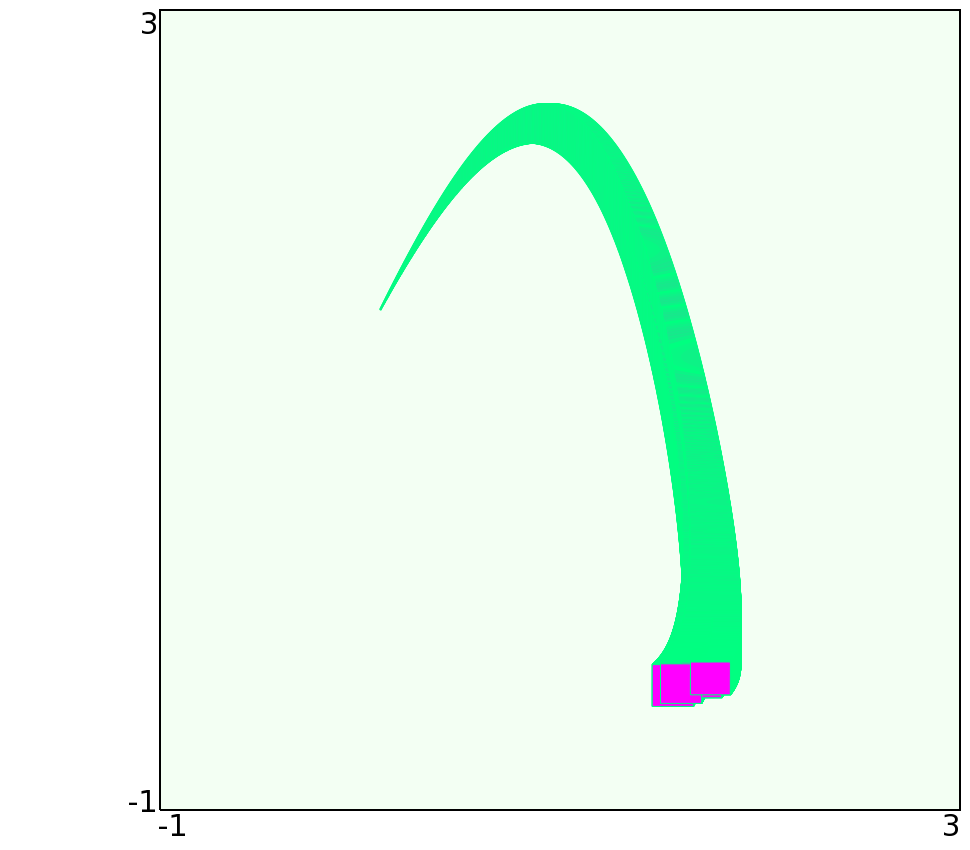
Figure 1: Evolution of the Perturbed Van der Pol Oscillator: splitting performed at $t_{1}=0.6$ and $t_{2}=1.2$.

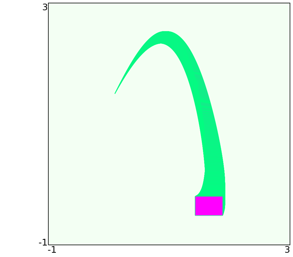
Figure 2: Evolution of the Perturbed Van der Pol Oscillator: no splitting performed.

Figures 2 and 2 show that our method is effective in practice for computing rigorous over-approximations of the solution sets of nonlinear differential inclusions. To prove this, we compare the results of computation of the algorithm presented here with the ones given in [17].

6.2 Perturbed Harmonic Oscillator

The equations for the perturbed harmonic oscillator are given by

$$\dot{x}=y+v_{1}$$

$$\dot{y}=-x+v_{2},$$

where $v_{i}$’s represent bounded noise. Suppose that the range of $v_{1}$ and $v_{2}$ is $[-A_{1},A_{1}]$ and $[-A_{2},A_{2}]$ respectively. Notice that noise is additive, and therefore we can use formula (32) to compute the (analytical) error. In terms of our general set up we have $f(x,y)=(y,-x)$, $g_{i}=1$, for $i=1,2$. Hence, we get $\Lambda=1$, $L=1$, $H=0$, and $K^{\prime}=A_{1}+A_{2}$. The one step time error is then given by the following formula

$$\epsilon=\frac{7\,h^{3}\,}{4(2-h)}\,\frac{e^{h}-1}{h}\,\max\{A_{1},A_{2}\}.$$

For comparison purposes, Table 2 is equivalent to a table given in [17]. The total time of computation is $T=2\pi$, $A_{1}=0$, and initial condition is the box $(1,0)+[-\delta,\delta]^{2}$. Note that diameter of the set $[a_{1},a_{2}]\times[b_{1},b_{2}]\in\mathbb{R}^{2}$ is $\max\{a_{2}-a_{1},b_{2}-b_{1}\}$, and radius of the set is half of diameter.

From Table 2, one can see that in most cases our results are better then one obtained in [17]. In case 2, the time step is $h=2\pi/9=0.698131$, for which the analytical error $\epsilon=0.066170$ is too large to hope for sharp results. In case 2, handling the large number of time steps requires more sophisticated techniques for simplifying the representation of the intermediate sets than are currently used in our code, and this is the major contribution to the error.

Table 2: Perturbed Harmonic Oscillator $T=2\pi$

case	$A_{2}$	$\delta$	num. of steps	Our Diameter	Diameter in [17]
1	0.1	0.01	9	3.91258	1.178825
2	0.1	0.01	100	0.8382630	0.8453958
3	0.1	0.01	1000	65.4376	0.8225159
4	0.1	0	100	0.8186080	0.8253958
5	0.1	0.01	100	0.8382630	0.8453958
6	0.1	0.1	100	1.018708	1.025396
7	0.01	0.01	100	0.1018380	0.1025396
8	0.1	0.01	100	0.8382630	0.8453958
9	1	0.01	100	8.205280	8.273958

When both $A_{1}$ and $A_{2}$ are nonzero, i.e. $A_{1}=A_{2}=0.1$, our results and results from [17] are given in Table 3. Here, we present results only for smaller time steps, even though in [17] the results were given for time steps up to $h=0.799$. We give both second-order and third-order local error estimates. We can see from Table 3 that for $h=0.25$ we are starting to get significantly worse results then in [17], but for smaller time steps the results are comparable. Here, the total time of computation is $T=h$ (one time step), and $\delta=0$.

Table 3: Perturbed Harmonic Oscillator $T=h$

case	h	Our Radius(2)	Our Radius(3)	Radius in [17]
1	0.25	0.0420586	0.0313667	0.0284025
2	0.1	0.0125864	0.0108419	0.0105171
3	0.01	0.00102509	0.00100759	0.00100502
4	0.001	0.00010026	0.00010009	0.00010005

We see that the radius of the enclosure is dominated by the growth due to the noise in the differential inclusion. The reason why our third-order error estimates give worse enclosures than those of [17] is unclear; however we note that the error estimates obtained there were computed exactly by hand, and our automated methods are better than those of [17] based on the logarithmic norm. Moreover, in [17] they use the 2-norm for the logarithmic norm which gives better results for this example.

6.3 Rossler Equations

The Rossler equations are given by

$$\dot{x} =-(y+z)+v_{1}$$

$$\dot{y} =x+0.2y+v_{2}$$

$$\dot{z} =0.2+z(x-a)+v_{3}$$

We aim to estimate the image of the initial set

$$X_{0}=\{0\}\times[-10.3\times 10^{-4},+10.3\times 10^{-4}]\times[-0.03\times 10^{-4},+0.03\times 10^{-4}]$$

under the return map $P$ to the Poincaré section $\Sigma=\{x=0,\,\dot{x}>0\}$ for the parameter value $a=5.7$ and noise $v_{i}\in[-10^{-4},10^{-4}]$ for $i=1,2,3$. Rather than compute the crossing time for each trajectory, we computed a time interval $T$ containing the first crossing time by comparing the sign of $x$ over the sets $R_{k}$, and used the estimate $\{0\}\times P(X_{0})\subset R(X_{0},T)$.

With time step $h=0.005$, total time $T=11.1$, and region of computation $D=([-25,25],[-25,25],[-25,35])$, we obtain an analytical error of $e=8.586\cdot 10^{-8}$ and

$$R(X_{0},T)=([-0.15572,0.15391],[-3.75926,-3.41772],[0.03139,0.03398]).$$

In [17], $R(X_{0},T)=([-0.211150,0.20888],[-3.69781,-3.47352],[0.03117,0.03327])$. (They did not specify the time step or the total time it took to compute the value of the poincare map $R(X_{0},T)$.) In this case neither of the sets is better then other, but they are comparable, and hence we show that our algorithm can also provide good estimates when computing over rather difficult regions, see [17].

7 Concluding Remarks

In this paper, we have given a numerical method for computing rigorous over-approximations of the reachable sets of differential inclusions. The method gives high-order error bounds for single-step approximations, which is an improvement of the first-order methods previously available. By providing improved control of local errors, the method allows for accurate computation of reachable sets over longer time intervals.

We give several theorems for obtaining local errors of different orders. It is easy to see that higher order errors (improved accuracy) require approximations that have larger number of parameters (reduced efficiency). The growth of the number of parameters is an issue, in general. Sophisticated methods for handling this are at least as important as the single-step method. The question remains as to approximate solution (Theorems 8-17) yields the best trade-off between local accuracy and efficiency for computing reachable sets. The answer is not straightforward and most likely depends on the system itself. In future work, we plan to investigate the efficiency of the algorithm on the number of parameters for various examples.

We have only considered differential inclusions in the form of input-affine systems, and give a brief sketch of how these methods can be applied to other classes of system. We also plan to provide a more detailed exposition of the method in these cases. Moreover, the local error that we obtain is a uniform bound for the error in all components. It should be possible to give slightly better componentwise bounds.

8 ACKNOWLEDGEMENTS

This research was partially supported by the European Commission through the project “Control for Coordination of Distributed Systems” (C4C) as part of the EU.ICT program (challenge ICT-2007.3.7).

References

• [1] Ariadne. http://trac.parades.rm.cnr.it/ariadne/
• [2] Aubin, J.P., and A., Cellina, Differential inclusions. Set-valued maps and viability theory. Grundlehren der Mathematischen Wissenschaften [Fundamental Principles of Mathematical Sciences], 264. Springer-Verlag, Berlin, 1984.
• [3] Baier, R., and Gerdts, M., A Computational Method for Non-Convex Reachable Sets Using Optimal Control. Proceedings of the European Control Conference 2009, Budapest, Hungary, 2009, 97-102
• [4] Beyn, W.-J., and Rieger, J., Numerical fixed grid methods for differential inclusions. (English summary) Computing. 81 (2007), no. 1, 91-106.
• [5] Collins, P., and Graca, D. S. Effective computability of solutions of differential inclusions: the ten thousand monkeys approach. J.UCS 15 (2009), no. 6, 1162-1185.
• [6] Collins, P., Niqui, M., and Revol, N., A Taylor Function Calculus for Hybrid System Analysis: Validation in Coq NSV-3: Third International Workshop on Numerical Software Verification. 2010.
• [7] Dahlquist, G. Stability and Error Bounds in the Numerical Integration of Ordinary Differential Equations, Almqvist and Wiksells, Uppsala, 1958; Transactions of the Royal Institute of Technology, Stockholm, 1959.
• [8] Deimling, K., Multivalued differential equations. De Gruyter Series in Nonlinear Analysis and Applications, 1. Walter de Gruyter and Co., Berlin, 1992.
• [9] Dontchev, A.; Lempio, F., Difference methods for differential inclusions: a survey. SIAM Rev. 34 (1992), no. 2, 263-294.
• [10] Dontchev, T. Euler approximation of nonconvex discontinuous differential inclusions. (English summary) An. Stiint. Univ. Ovidius Constanta Ser. Mat. 10 (2002), no. 1, 73–86.
• [11] Dontchev, A. L.; Farkhi, E. M. Error estimates for discretized differential inclusion. Computing. 41 (1989), no. 4, 349-358.
• [12] Filippov, A. F. Differential equations with discontinuous righthand sides. Translated from the Russian. Mathematics and its Applications (Soviet Series), 18. Kluwer Academic Publishers Group, Dordrecht, 1988.
• [13] Fliess, M., Fonctionnelles causales non linéaires et indéterminés non commutatives. Bull. Soc. Math. France 109 (1981), 3-40.
• [14] Grammel, G., Towards fully discretized differential inclusions. Set-Valued Anal. 11 (2003), no. 1, 1-8.
• [15] Grüne, L., Kloeden, P. E., Higher order numerical schemes for affinely controlled nonlinear systems. Numer. Math. 89 (2001), no. 4, 669–690.
• [16] Hairer, E.; Nørsett, S. P.; Wanner, G. Solving ordinary differential equations. I. Nonstiff problems. Springer Series in Computational Mathematics, 8. Springer-Verlag, Berlin, 1987
• [17] Kapela, T. A.; Zgliczynski, P., A Lohner-type algorithm for control systems and ordinary differential inclusions. Discrete Contin. Dyn. Syst. Ser. B 11 (2009), no. 2, 365–385.
• [18] Li, Desheng. Morse decompositions for general dynamical systems and differential inclusions with applications to control systems. SIAM J. Control Optim. 46 (2007), no. 1, pp. 35-60.
• [19] Lozinskii, S.M. Error estimates for the numerical integration of ordinary differential equations, part I, Izv. Vyss. Uceb. Zaved Matematika, 6 (1958), pp. 52–90 (Russian).
• [20] Kurzhanski, A.; Valyi, I., Ellipsoidal calculus for estimation and control. (English summary) Systems and Control: Foundations and Applications. Birkhäuser Boston, Inc., Boston, MA; International Institute for Applied Systems Analysis, Laxenburg, 1997.
• [21] Makino, K., and Berz, M., Taylor Models and Other Validated Functional Inclusion Methods. International Journal of Pure and Applied Mathematics 4 (2003), no. 4, 379-456
• [22] Nieuwenhuis, J. W. Some remarks on set-valued dynamical systems. J. Austral. Math. Soc. Ser. B 22 (1981), no. 3, pp. 308-313.
• [23] Puri, A.; Borkar, V. and Varaiya, P., $\epsilon$-approximation of differential inclusions, Proc. of the 34th IEEE Conference on Decision and Control (1995), pp. 2892–2897.
• [24] Revol, N.; Makino, K.; Berz, M. Taylor models and floating-point arithmetic: proof that arithmetic operations are validated in COSY. J. Log. Algebr. Program. 64 (2005), no. 1, 135–154.
• [25] Smirnov, G. V., Introduction to the theory of differential inclusions. Graduate Studies in Mathematics, 41. American Mathematical Society, Providence, RI, 2002.
• [26] Söderlind, G. The logarithmic norm. History and modern theory. (English summary) BIT 46 (2006), no. 3, 631–652.
• [27] Wade, R. W., An Introduction to Analysis. Pearson Prentice Hall, Upper Saddle River, NJ, 2009.
• [28] Weihrauch, K., Computable analysis. An introduction. Texts in Theoretical Computer Science. An EATCS Series. Springer-Verlag, Berlin, 2000.