Evaluation of the importance of spin-orbit couplings in the nonadiabatic quantum dynamics with quantum fidelity and with its efficient “on-the-fly” ab initio semiclassical approximation

Abstract

We propose to measure the importance of spin-orbit couplings (SOCs) in the nonadiabatic molecular quantum dynamics rigorously with quantum fidelity. To make the criterion practical, quantum fidelity is estimated efficiently with the multiple-surface dephasing representation (MSDR). The MSDR is a semiclassical method that includes nuclear quantum effects through interference of mixed quantum-classical trajectories without the need for the Hessian of potential energy surfaces. Two variants of the MSDR are studied, in which the nuclei are propagated either with the fewest-switches surface hopping or with the locally mean field dynamics. The fidelity criterion and MSDR are first tested on one-dimensional model systems amenable to numerically exact quantum dynamics. Then, the MSDR is combined with “on-the-fly” computed electronic structure to measure the importance of SOCs and nonadiabatic couplings (NACs) in the photoisomerization dynamics of CH₂NH₂⁺ considering 20 electronic states and in the collision of F + H₂ considering six electronic states.

I Introduction

Nonadiabatic couplings (NACs) originating in the Born-Oppenheimer separation of motion of electrons and nuclei often play an important role in the molecular dynamics.Child and Robb (2004) In photochemistry, NACs are responsible for radiationless decay of the electronically excited states by a process called internal conversion.Worth and Cederbaum (2004); Martinez (2010) In chemical reaction dynamics, they may affect branching ratios of product channels or allow for reactivity of otherwise nonreactive states, when the transition from a nonreactive potential energy surface (PES) to a reactive PES is induced by the motion of nuclei.Butler (1998); Wu (2010) In some cases, transitions between PESs may be induced by another type of couplings called spin-orbit couplings (SOCs), which couple the electronic spin with angular momentum.Marian (2012) Relativistic in origin, SOCs become increasingly important in molecules containing heavy elements. Nevertheless, SOCs often play a role also in molecules composed of light elements, e.g., various chromophores or DNA bases.González-Luque et al. (2010) In photochemistry, SOCs cause radiationless transitions between PESs of different multiplicity called intersystem crossings, which are responsible for the phosphorescence or emergence of triplet intermediates in photochemical reactions.Neiss and Saalfrank (2003); Griesbeck et al. (2004); Abe et al. (2004) Similarly to NACs, SOCs may affect chemical reactions even when no photoexcitation is involved.Maiti et al. (2004); Lique et al. (2011)

Even though intersystem crossing is typically slower than internal conversion in molecules composed of light elements, in some cases both effects may occur on a comparable time scale.Takezaki et al. (1998); Satzger et al. (2004); Reichardt et al. (2009); Minns et al. (2010) Therefore, there is a need for a rigorous criterion of the importance of SOCs in accurate quantum nonadiabatic simulations. Knowing in advance which PESs and which couplings are important for given initial conditions may speed up a simulation and avoid costly calculations of additional PESs. Below, we propose and test a criterion of importance of SOCs which is based on the quantum fidelity.Peres (1984) In a similar manner, fidelity was already used to measure nondiabaticityZimmermann and Vaníček (2010) or nonadiabaticityMacKenzie et al. (2012); Zimmermann and Vaníček (2012) of quantum dynamics. However, direct evaluation of fidelity requires knowledge of the quantum state evolved with the complete Hamiltonian including SOCs and consequently is impractical as a guide for quantum simulations. Fortunately, there exists a fast semiclassical method to compute quantum fidelity, called the multiple-surface dephasing representation (MSDR).Zimmermann and Vaníček (2010, 2012) Evaluation of the importance of SOCs with the MSDR is the main focus of this work.

Originally, the MSDR was introduced to measure either the nonadiabaticity or nondiabaticity of the quantum molecular dynamics.Zimmermann and Vaníček (2010, 2012) Roughly speaking, “nondiabaticity” is the difference between the diabatic quantum dynamics (i.e., quantum dynamics in which the diabatic coordinate couplings between diabatic electronic surfaces are neglected) and the fully coupled quantum dynamics. Similarly, “nonadiabaticity” is the difference between the adiabatic quantum dynamics (i.e., quantum dynamics in which the nonadiabatic momentum couplings between adiabatic electronic surfaces are neglected) and the fully coupled quantum dynamics. In both cases the “difference” between the two types of dynamics is measured by the decay of the overlap of the time-dependent molecular wave functions evolved using the two types of dynamics. In the same manner, the importance of SOCs may be evaluated either in: 1) the basis which is diabatic with respect to SOCs, meaning that the Hamiltonian matrix expressed in this basis does not contain any spin-orbit-related couplings that depend on the nuclear momentum, or 2) in the basis which is adiabatic with respect to SOCs, meaning that the only spin-orbit-related couplings present in the Hamiltonian depend on the nuclear momentum. The basis which is diabatic with respect to SOCs is usually more suitable when SOCs represent only a small perturbation, whereas the basis which is adiabatic with respect to SOCs is more appropriate in case of strong coupling. Independently of the adiabaticity or diabaticity with respect to SOCs, the basis may be adiabatic or diabatic with respect to couplings originating in the Born-Oppenheimer separation of motion of electrons and nuclei. Below, we use exclusively the basis which is diabatic with respect to SOCs. When analyzing the importance of SOCs, we always evaluate the importance of the full spin-orbit Hamiltonian which may include diagonal terms as well. Nevertheless, the fidelity criterion and MSDR may be used also in the fully adiabatic basis of spin-orbit states, which is employed, for example, in the mixed quantum-classical code SHARC.Richter et al. (2011) It is important to note that spin-orbit-related couplings have different meaning in the two basis sets. In the diabatic basis with respect to SOCs, when the full spin-orbit Hamiltonian is considered as a perturbation, SOCs reflect faithfully the importance of the spin-orbit interaction in the system. In the adiabatic basis with respect to SOCs, on the other hand, the spin-orbit interaction modifies the PESs themselves and the lack of importance of the offdiagonal spin-orbit-related couplings does not necessarily mean that the spin-orbit interaction is unimportant.

The MSDR is a generalization to nonadiabatic dynamics of the dephasing representation (DR),Vaníček and Heller (2003); Vaníček (2004, 2006) derived for dynamics on a single surface using the Van Vleck propagator or the linearization of the path integral.Shi and Geva (2004) In the single-surface setting, the DR is closely related to the semiclassical perturbation approximation of Smith, Hubbard, and MillerMiller and Smith (1978); Hubbard and Miller (1983) and to the phase averaging of Mukamel.Mukamel (1982) Its applications include evaluations of the stability of quantum dynamicsVaníček (2004, 2006); Gorin et al. (2006); Wisniacki et al. (2010); García-Mata et al. (2011) and calculations of electronic spectra.Mukamel (1982); Rost (1995); Li et al. (1996); Egorov et al. (1998); Shi and Geva (2005); Wehrle et al. (2011); Šulc and Vaníček (2012)

While the MSDR is not a method for general dynamics, it can be used to compute all quantities which can be expressed in terms of quantum fidelity amplitude. Weaker generality and semiclassical nature give the MSDR some advantages in comparison to general methods for nonadiabatic dynamics.

The main advantage of the MSDR compared to wave packet methods is that the number of trajectories needed for convergence of MSDR does not scale exponentially with the number of degrees of freedom.Mollica and Vaníček (2011) Therefore, the MSDR may be applied to problems with dimensionality beyond the scope of even the most advanced methods for nonadiabatic quantum dynamics such as the multi-configuration time-dependent Hartree methods.Meyer et al. (2009); Worth et al. (2008); Burghardt et al. (2008); Blancafort et al. (2011) Similarly to other semiclassical methods,Martínez et al. (1996); Yang et al. (2009); Burant and Batista (2002); Kondorskiy and Nakamura (2004); Wu and Herman (2005); Sun and Miller (1997); Miller (2009); Heller et al. (2002) the MSDR includes some quantum effects on the nuclear motion. The advantage of MSDR in comparison to most other semiclassical approaches is that the MSDR does not require the Hessian of the potential energy, which is often the most expensive part of semiclassical calculations (see, e.g., Ref. Ceotto et al., 2009). In terms of the computational cost per trajectory, the MSDR thus falls into the category of methods in which nuclei are treated classically such as surface hopping methods,Tully (1990); Nielsen et al. (2000); Shenvi (2009) and other methods based on the mixed quantum-classical Liouville equation,Donoso and Martens (1998); Kapral and Ciccotti (1999); Horenko et al. (2002); Ando and Santer (2003); Horenko et al. (2004); Micha and Thorndyke (2004); Mac Kernan et al. (2008); Bonella et al. (2010); Bousquet et al. (2011) or methods obtained by linearization of the path integral expression for the quantum propagator.Dunkel et al. (2008); Huo and Coker (2011) (Costs of current implementations of the MSDR are essentially the costs of a mean field or surface hopping dynamics. Nevertheless, in principle, the MSDR may be combined with a propagation scheme based directly on the mixed quantum-classical Liouville equation, which is typically more expensive but also more accurate.)

The outline of the paper is as follows: Section II starts by introducing the fidelity criterion of importance of SOCs and by defining the spin-orbit Hamiltonian. This is followed by a brief derivation of the MSDR, and the description of the propagation scheme and the algorithm. The section ends with the computational details. In Section III, the fidelity criterion and MSDR are tested using one-dimensional model systems which allow for numerically exact quantum solution. Subsequently, the MSDR is combined with “on-the-fly” computed ab initio electronic structure and applied to evaluate the importance of SOCs and NACs in the photoisomerization of CH₂NH₂⁺ and in the collision of F + H₂. Section IV concludes the paper.

II Theory

II.1 Fidelity as a measure of importance of spin-orbit coupling terms

Following our work on the nondiabaticityZimmermann and Vaníček (2010) and nonadiabaticityZimmermann and Vaníček (2012) of the molecular dynamics we base the quantitative criterion of importance of SOCs on quantum fidelity $F_{\mathrm{QM}}$ between molecular quantum states propagated with and without SOCs. More precisely,

$$F_{\mathrm{QM}}(t)=|f_{\mathrm{QM}}(t)|^{2}=|\langle\psi^{0}(t)|\psi^{\epsilon}(t)\rangle|^{2},$$ (1)

where $f_{\mathrm{QM}}$ is the quantum fidelity amplitude, $\left|\psi^{0}(t)\right\rangle=e^{-i\mathbf{\hat{H}}^{0}t/\hbar}\left|\psi(0)\right\rangle$ is the quantum state of the molecule evolved using the nonadiabatic Hamiltonian $\mathbf{\hat{H}}^{0}$ which does not include SOCs of interest and $|\psi^{\epsilon}(t)\rangle=e^{-i\mathbf{\hat{H}}^{\epsilon}t/\hbar}\left|\psi(0)\right\rangle$ is the quantum state evolved using the fully coupled nonadiabatic Hamiltonian $\mathbf{\hat{H}}^{\epsilon}=\mathbf{\hat{H}}^{0}+\epsilon\hat{\mathbf{V}}$. In the last expression, $\hat{\mathbf{V}}=\mathbf{\hat{H}}^{\text{SO}}$ contains SOCs of interest and $\epsilon$ controls the extent of perturbation. (Bold face denotes $n\times n$ matrices acting on the Hilbert space spanned by $n$ electronic states, hat $\hat{}$ denotes nuclear operators. In general, the superscript $0$ or $\epsilon$ designates the Hamiltonian with which the object was propagated.) When $F_{\mathrm{QM}}\approx 1$, $\left|\psi^{0}(t)\right\rangle$ is close to $\left|\psi^{\epsilon}(t)\right\rangle$ and SOCs do not influence the dynamics significantly. On the other hand, when $F_{\mathrm{QM}}\ll 1$, SOCs are important and should be taken into account in an accurate quantum calculation. The advantage of the fidelity criterion is that, in addition to population transfer between PESs (which is a standard dynamical measure of the importance of couplings), fidelity can detect subtle effects on the dynamics caused by the displacement and interference on a single PES (see Ref. Zimmermann and Vaníček, 2012 for details).

II.2 Spin-orbit Hamiltonian

In principle, any spin-orbit coupling Hamiltonian $\mathbf{\hat{H}}^{\text{SO}}$ may be used. In this work, model potentials are used in one-dimensional systems. In case of the photoisomerization of CH₂NH₂⁺ and collision of F + H₂, elements of $\mathbf{\hat{H}}^{\text{SO}}$ are computed with the Breit-Pauli HamiltonianBerning et al. (2000)

$$\hat{H}^{\mathrm{BP}} = \sum_{j,J}\frac{Z_{J}\left(\hat{q}_{jJ}\times\hat{p}_{j}\right)\cdot\hat{s}_{j}}{2c^{2}\left|q_{jJ}\right|^{3}}$$ (2)

$$-\sum_{j\neq k}\left[\frac{\left(\hat{q}_{kj}\times\hat{p}_{j}\right)\cdot\hat{s}_{j}}{2c^{2}\left|q_{jk}\right|^{3}}+\frac{\left(\hat{q}_{jk}\times\hat{p}_{k}\right)\cdot\hat{s}_{j}}{c^{2}\left|q_{jk}\right|^{3}}\right],$$

where $\hat{q}_{jJ}=(\hat{q}_{j}-\hat{Q}_{J})$ is the difference of position vectors of electron $j$ and nucleus $J$, $\hat{q}_{jk}=(\hat{q}_{j}-\hat{q}_{k})$ is the difference of position vectors of of electron $j$ and $k$, $\hat{p}_{j}$ is the momentum of electron $j$, and $\hat{s}_{j}$ is the spin of electron $j$. Exceptionally, since $\hat{H}^{\mathrm{BP}}$ is not expressed in any basis yet, in Eq. (2) (and only there) hats denote both electronic and nuclear operators.

II.3 MSDR

Here we will only summarize the theory of MSDR; the full derivation may be found in Ref. Zimmermann and Vaníček, 2012. The derivation starts with a quantum fidelity amplitude expression generalized to the Hilbert space given by the tensor product $\mathbb{C}^{n}\otimes\mathcal{L}^{2}\left(\mathbb{R}^{D}\right)$:Vaníček (2006)

$$f_{\mathrm{QM}}\left(t\right)=\mathrm{Tr}\left(e^{-i\mathbf{\hat{H}}^{\epsilon}t/\hbar}\cdot\mathbf{\mathbf{\boldsymbol{\hat{\rho}}}}^{\text{init}}\cdot e^{+i\mathbf{\hat{H}}^{0}t/\hbar}\right),$$ (3)

where $\boldsymbol{\hat{\rho}}^{\text{init}}$ is the density operator of the initial state. Expressing $f_{\mathrm{QM}}$ in the interaction picture and partially Wigner transformingWigner (1932) the resulting equation over nuclear degrees of freedom yields an alternative exact expression

$$f_{\mathrm{QM}}\left(t\right) =h^{-D}\mathrm{Tr}_{e}\int d^{2D}X\boldsymbol{\rho}_{\text{W}}^{\text{init}}\left(X\right)\cdot\left({\cal T}e^{-i\epsilon\int_{0}^{t}\mathbf{\hat{V}}^{\text{I}}\left(t^{\prime}\right)dt^{\prime}/\hbar}\right)_{\text{W}},$$ (4)

where $X$ denotes the point $(Q,P)$ in the $2D$-dimensional nuclear phase space, $\mathrm{Tr}_{e}$ is the trace over electronic degrees of freedom, and $\mathbf{\hat{V}}^{\text{I}}\left(t\right)$ is the perturbation in the interaction picture given by $\mathbf{\hat{H}}^{0}$. The first approximation consists in replacing the Wigner transform of a product of operators in the Taylor expansion of the time-ordered exponential in Eq. (4) by the product of Wigner transforms of these operators. Recognizing the resulting sum as an Taylor expansion of another exponential, this approximation can be expressed succinctly as

$$\left({\cal T}e^{-i\epsilon\int_{0}^{t}\mathbf{\hat{V}}^{\text{I}}\left(t^{\prime}\right)dt^{\prime}/\hbar}\right)_{\text{W}}\simeq{\cal T}e^{-i\epsilon\int_{0}^{t}\mathbf{V}_{\text{W}}^{\text{I}}\left(X,t^{\prime}\right)dt^{\prime}/\hbar}.$$ (5)

To evaluate this expression, the time evolution of $\mathbf{V}_{\text{W}}^{\text{I}}\left(X,t\right)$ has to be known. The second approximation involves replacing the exact evolution by a mixed quantum-classical (MQC) propagation scheme described below, leading to the final expression for the MSDR of fidelity amplitude,

$$f_{\text{MSDR}}(t)=\left\langle{\cal T}e^{-i\epsilon\int_{0}^{t}\mathbf{V}_{\text{W,MQC}}^{\text{I}}\left(X,t^{\prime}\right)dt^{\prime}/\hbar}\right\rangle_{\boldsymbol{\rho}_{\text{W}}^{\text{init}}\left(X\right)}\\ =h^{-D}\mathrm{Tr}_{e}\int d^{2D}X\boldsymbol{\rho}_{\text{W}}^{\text{init}}(X)\cdot{\cal T}e^{-i\epsilon\int_{0}^{t}\mathbf{V}_{\text{W,MQC}}^{\text{I}}\left(X,t^{\prime}\right)dt^{\prime}/\hbar}.$$ (6)

II.4 Propagation scheme

The MQC equationAleksandrov (1981); Boucher and Traschen (1988); Martens and Fang (1997); Prezhdo and Kisil (1997); Kapral and Ciccotti (1999); Caro and Salcedo (1999); Shi and Geva (2004) for the evolution of the density matrix is given by

$$\frac{\partial\boldsymbol{\rho}_{\text{W,MQC}}}{\partial t}=-\frac{i}{\hbar}\left[\mathbf{H}_{\text{W}},\boldsymbol{\rho}_{\text{W,MQC}}\right]\\ +\frac{1}{2}\left(\left\{\mathbf{H}_{\text{W}},\boldsymbol{\rho}_{\text{W,MQC}}\right\}-\left\{\boldsymbol{\rho}_{\text{W,MQC}},\mathbf{H}_{\mathrm{\text{W}}}\right\}\right),$$ (7)

where the explicit dependence of $\boldsymbol{\rho}_{\text{W,MQC}}$ on time and on the nuclear phase-space coordinate $X$ was omitted for clarity. The propagation equation for $\mathbf{V}_{\text{W,MQC}}^{\text{I}}\left(X,t\right)$, which is the last ingredient needed in our method, differs from Eq. (7) only by the sign of the time derivative. Therefore Eq. (6) together with Eq. (7) define the MSDR. Several numerical approaches exist that solve Eq. (7) in terms of “classical” trajectories $X(t)$. However, since trajectory-based methods for solving Eq. (7) are still relatively complicated, the MSDR is in practice implemented using one of two schemes which further approximate Eq. (7). The common feature of the two approximations is that all elements of $\boldsymbol{\rho}_{\text{W}}\left(X,t\right)$ are propagated using the same PES (which may, nevertheless, differ for different trajectories). The first approachZimmermann and Vaníček (2012) approximates Eq. (7) as

$$\frac{\partial\boldsymbol{\rho}_{\text{W,LMFD}}}{\partial t}=-\frac{i}{\hbar}\left[\mathbf{H}_{\text{W}},\boldsymbol{\rho}_{\text{W,LMFD}}\right]\\ +\frac{\partial\boldsymbol{\rho}_{\text{W,LMFD}}}{\partial P}\left\langle\frac{\partial\mathbf{H}_{\text{W}}}{\partial Q}\right\rangle_{e}-\frac{\partial\boldsymbol{\rho}_{\text{W,LMFD}}}{\partial Q}\frac{P}{M},$$ (8)

where $\left\langle\mathbf{A}\right\rangle_{e}=\mathrm{Tr}_{e}\left(\boldsymbol{\rho}_{e}\cdot\mathbf{A}\right)$ is a partial average of $\mathbf{A}$ over the electronic subspace. This approach was called the locally mean field dynamics (LMFD) in Ref. Zimmermann and Vaníček, 2012, where it was derived simply by invoking the locally mean field approximation. As pointed out in Ref. Zimmermann and Vaníček, 2012, the LMFD turns out to be nothing else than the dynamics of a swarm of trajectories, each of which is propagated with the Ehrenfest dynamics. The second approach employs the physically motivated fewest-switches surface hopping (FSSH) scheme,Tully (1990) where the matrix elements of the density operator $\boldsymbol{\rho}_{\text{W,FSSH}}$ are (in the adiabatic basis) computed using Eq. (11) of Ref. Tully, 1990.

II.5 Algorithm

The details of the general implementation of the MSDR algorithm are given in Ref. Zimmermann and Vaníček, 2012. In this work, we consider only initial states for which the “conditional” electronic density matrix is pure for all $X$ and hence the initial density matrix can be written as the tensor product

$$\boldsymbol{\rho}_{\text{W}}^{\text{init}}\left(X\right)=\rho^{\text{init}}\left(X\right)\mathbf{c^{\mathrm{init}}}\left(X\right)\otimes\mathbf{c}^{\mathrm{init}}\left(X\right)^{\dagger}$$ (9)

where $\rho^{\text{init}}\left(X\right):=\mathrm{Tr}_{e}\boldsymbol{\rho}_{\mathrm{W}}^{\text{init}}\left(X\right)$ and $\mathbf{c^{\mathrm{init}}}\left(X\right)$ is the initial electronic wave function for nuclei located at $X$. In practice, $N_{\text{traj}}$ phase space points are sampled from a scalar nuclear density $\rho^{\text{init}}(X)$ and a vector $\mathbf{c^{\mathrm{init}}}\left(X\right)$ is attributed to each of the generated phase space points. In the case of LMFD, this determines the initial condition completely. In the case of FSSH, one also needs to select the initial surface randomly and separately for each trajectory according to the following prescription: For a trajectory starting at $X$, the probability for its initial surface to be surface $j$ is given by $\left|c_{j}^{\text{init}}(X)\right|^{2}$. The trajectories are then propagated with $\mathbf{H}_{\text{W}}^{0}$ [because, ultimately, we propagate $\mathbf{V}_{\text{W,MQC}}^{\text{I}}\left(X,t\right)$ in the interaction picture given by $\mathbf{H}_{\text{W}}^{0}$] by using either the LMFD or FSSH dynamics. It is advantageous that for states (9), when the LMFD or FSSH dynamics is used, Eq. (6) simplifies to the weighted phase space average

$$f_{\text{MSDR}}\left(t\right)=\left\langle\mathbf{c}^{0}\left(X,t\right)^{\dagger}\cdot\mathbf{c}^{\epsilon}\left(X,t\right)\right\rangle_{\rho^{\text{init}}\left(X\right)}.$$ (10)

In Eq. (10), the wave function $\mathbf{c}^{0}\left(X,t\right)$ is obtained automatically from the LMFD or FSSH dynamics. Analogously, $\mathbf{c}^{\epsilon}\left(X,t\right)$ solves the Schrödinger equation

$$\frac{\partial\mathbf{c}^{\epsilon}\left(X,t\right)}{\partial t}=-\frac{i}{\hbar}\mathbf{H}_{\text{W}}^{\epsilon}(X^{0}(t))\cdot\mathbf{c}^{\epsilon}\left(X,t\right)$$ (11)

for a single discrete electronic degree of freedom with a time-dependent Hamiltonian $\mathbf{H}_{\text{W}}^{\epsilon}(t):=\mathbf{H}_{\text{W}}^{\epsilon}(X^{0}(t))$ (i.e., in the Lagrangian reference frame given by $\mathbf{H}_{\text{W}}^{0}$) and with the initial condition $\mathbf{c}^{\epsilon}\left(X,0\right)=\mathbf{c}^{\mathrm{init}}\left(X\right)$. In Eq. (11), $X^{0}(t)$ is the phase space point resulting from the evolution of the initial phase space point $X$ for time $t$ with $\mathbf{H}_{\text{W}}^{0}$, using either the LMFD or FSSH dynamics.

II.6 Computational details

All quantum calculations were performed using the second-order split-operator algorithm.Feit and Fleck (1983) The LMFD or FSSH dynamics were done using the second-order symplectic Verlet integrator.Verlet (1967) The Schrödinger equation for the discrete “electronic” degree of freedom was solved using the unitary propagator $\mathbf{U}(X,t,t+\Delta t)=e^{-i\mathbf{H}_{\text{W}}\left(X\right)\Delta t/\hbar}$. Ab initio calculations were performed using Molpro 2010.1Werner et al. (2010) and Columbus 5.9.2.Lischka et al. (2010)

III Results

III.1 Comparison of the MSDR with the numerically exact quantum dynamics

In order to test the utility of quantum fidelity as a measure of the importance of SOCs and the performance of the MSDR in comparison to the numerically exact quantum dynamics we use three one-dimensional model systems. Results are shown in Fig. 1.

The PESs and couplings of model A are shown in the right part of Fig. 1 (a). Both Hamiltonians $\mathbf{\hat{H}}^{0}$ and $\mathbf{\hat{H}}^{\epsilon}$ are expressed in the diabatic basis with respect to both SOCs and couplings originating in the Born-Oppenheimer separation of motion of electrons and nuclei. Both Hamiltonians contain three PESs, of which the lower two are identical to the PESs of Tully’s single avoided crossing model.Tully (1990) The third PES is flat with constant energy $E=0.15\,\mathrm{a.u.}$ In both Hamiltonians, the lower two PESs are coupled by the same coupling term $V_{12}$ as in the original single avoided crossing model. Additionally, in $\mathbf{\hat{H}}^{\epsilon}$ (but not in $\mathbf{\hat{H}}^{0}$), the highest PES is coupled to the lower two PESs with $V_{13}=V_{31}^{*}=V_{23}=V_{32}^{*}=\left(1+i\right)\left[C\exp\left(-DQ^{2}\right)\right],$ where $C=0.005$ and $D=1.0$. A more general, complex form was chosen to emulate spin-orbit coupling terms, which may also be complex-valued. The initial state is a Gaussian wave packet (GWP) located on the lowest energy PES with the mean kinetic energy $T_{0}=0.025$ $\mathrm{a.u.}$ As can be seen in Fig. 1 (a), quantum fidelity $F_{\mathrm{QM}}$ decays substantially (by more than 50%), signifying the importance of $V_{13}$ and $V_{23}$ in the dynamics. The decay of $F_{\mathrm{QM}}$ is accurately reproduced by the MSDR using both the LMFD and FSSH dynamics. On the other hand, the decay of the survival probability $P_{1+2,\text{QM}}=1-P_{3,\text{QM}}$ is very small and the final probability $P_{3,\text{QM}}$ of finding the system on the third PES is less than 1%. This demonstrates that the survival probability $P_{1+2,\text{QM}}$ may be a poor measure of the importance of couplings between PESs. More refined criteria, such as the fidelity criterion, are needed to measure the influence of SOCs. (Note that in this specific case, strong effects of couplings of the first two PESs to the third PES may be inferred from considering the probabilities P₁ and P₂ separately. However, for that it is necessary to run the dynamics twice - once with couplings to the third surface and once without the couplings. To use the fidelity criterion approximated by the MSDR only one simulation is sufficient.)

Model B shown in Fig. 1 (b) is based on the two-surface Tully’s double avoided crossing model.Tully (1990) It is also expressed in the diabatic basis with respect to both SOCs and couplings originating in the Born-Oppenheimer separation of motion of electrons and nuclei. The third additional surface is described by the equation $V_{33}=FQ^{2}+G,$ where $F=-2\cdot 10^{-5}$ and $G=0.06$. The coupling term $V_{23}=V_{32}^{*}=iI\exp\left(-JQ^{2}\right)$ (with $I=0.003$ and $J=0.001$) is present only in $\mathbf{\hat{H}}^{\epsilon}$. As can be seen in the right part of Fig. 1 (b), the coupling term $V_{23}$ is relatively weak but widely spread, resembling closely SOCs typically seen in molecular dynamics. The initial state is a GWP located on the second lowest-energy PES with mean kinetic energy $T_{0}=0.368$ $\mathrm{a.u.}$ Again, the decay of $F_{\mathrm{QM}}$ is closely followed by both implementations of the MSDR. This time, even $P_{1+2,\text{QM}}$ follows $F_{\mathrm{QM}}$ relatively well. Still, the approximate MSDR method gives a slightly more accurate picture of the influence of SOCs on the dynamics.

Model C [Fig. 1 (c)], inspired by Tully’s extended coupling model,Tully (1990) demonstrates that the fidelity criterion detects the importance of SOCs even in cases where no significant transition of the probability density between surfaces occurs. The PESs and couplings are given by

$$V_{11}\left(Q\right) = -A$$

$$V_{22}\left(Q\geq 0\right) = A+B\exp\left(-CQ\right)$$

$$V_{22}\left(Q<0\right) = A+B\left[2-\exp\left(CQ\right)\right]$$

$$V_{12}\left(Q\geq 0\right) = B\left[2-\exp\left(-CQ\right)\right]$$

$$V_{12}\left(Q<0\right) = B\exp\left(CQ\right),$$

where $A=10$, $B=0.1,$ and $C=0.9$. The real-valued coupling term $V_{12}$ is present in $\mathbf{\hat{H}}^{\epsilon}$ but not in $\mathbf{\hat{H}}^{0}$. (Note that when the coupling term is purely imaginary, the results are exactly identical.) As can be seen in Fig. 1 (c), for a low energy wavepacket the wavefunctions propagated with $\mathbf{\hat{H}}^{0}$ and $\mathbf{\hat{H}}^{\epsilon}$ are very different. Indeed, fidelity decays towards zero. On the other hand, the survival probability $P_{1}$ never decays by more than $6\cdot 10^{-5}$. Even though the model is slightly artificial (in that the PESs are considerably coupled, despite a large energy difference between them), it clearly demonstrates the plausibility of situations in which the dynamical importance of SOCs would be undetectable if measured with the survival probability as a criterion. Finally, Fig. 1 (c) shows that the MSDR still closely follows the quantum result. [Since $\mathbf{\hat{H}}^{0}$ is uncoupled, both the LMFD and FSSH dynamics are equivalent. Therefore, only the FSSH result is shown in Fig. 1 (c).]

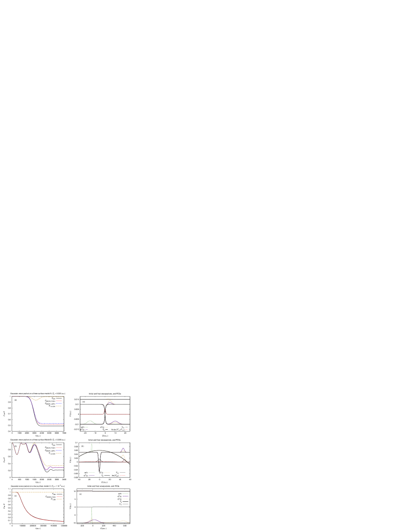
Figure 1: Importance of SOCs in the nonadiabatic dynamics: comparison with the numerically exact quantum dynamics on model systems. Left panels compare the quantum fidelity ($F_{\mathrm{QM}}$) with the MSDR ($F_{\mathrm{MSDR}}$) and with the quantum survival probability ($P_{\mathrm{QM}}$). Right panels show the corresponding diabatic PESs and couplings $V_{jj}(Q)$ as well as initial [$\psi(0)$] and final [$\psi^{0}(t_{f})$ and $\psi^{\epsilon}(t_{f})$] wave functions evolved with $\mathbf{\hat{H}}^{0}$ and $\mathbf{\hat{H}}^{\epsilon}$, respectively. In all three models, the initial state was the GWP $\psi(q)=\frac{1}{\sigma\sqrt{\pi}}\exp\left[-(Q-Q_{0})^{2}/2\sigma^{2}+P_{0}(Q-Q_{o})/\hbar\right]$ with the mass equal to 2000 $\mathrm{a.u.}$ (a) Coupling terms $V_{13}=V_{23}$, containing both real and imaginary parts, result in a very low decay of $P_{\mathrm{QM}}$ which does not correspond to the substantial decay of $F_{\mathrm{QM}}$. Only the lowest-energy PES was occupied initially by a GWP with $Q_{0}=-15$ $\mathrm{a.u.}$, $P_{0}=10$ $\mathrm{a.u.}$, and $\sigma=2.83$ $\mathrm{a.u.}$ (b) Extensive but relatively weak purely imaginary spin-orbit coupling term causes considerable decay of both $F_{\mathrm{QM}}$ and $P_{\mathrm{QM}}$. Only the second lowest-energy PES was occupied initially by a GWP with $Q_{0}=-15$ $\mathrm{a.u.}$, $P_{0}=38.36$ $\mathrm{a.u.}$, and $\sigma=0.74$ $\mathrm{a.u.}$ (c) The coupling term $V_{12}$ causes decay of $F_{\mathrm{QM}}$ towards zero without affecting $P_{\mathrm{QM}}$. Only the lowest-energy PES was occupied initially by a GWP with $Q_{0}=-20$ $\mathrm{a.u.}$, $P_{0}=0.2$ $\mathrm{a.u.}$, and $\sigma=3.41$ $\mathrm{a.u.}$

III.2 On-the-fly ab initio photoisomerization dynamics of CH₂NH₂⁺

As the first on-the-fly ab initio application of the MSDR, we examined the importance of SOCs and NACs in the quantum dynamics of the second excited singlet state of CH₂NH₂⁺ using the SA5,5-CASSCF(6,4)/6-31G* method. The time step of the FSSH dynamics was equal to $\sim 0.2$ $\mathrm{fs}$. In total, five lowest-energy singlet states and 15 lowest-energy triplet states (five states for each $M_{S}=1,0,-1$) were considered in the simulation. To evaluate the nonadiabaticity, the unperturbed Hamiltonian $\mathbf{\hat{H}}^{0}$ did not contain any couplings between surfaces and the perturbed Hamitonian $\mathbf{\hat{H}}^{\epsilon}$ contained NACs between singlet states. To evaluate the importance of SOCs, $\mathbf{\hat{H}}^{0}$ contained only NACs between singlet states while $\mathbf{\hat{H}}^{\epsilon}$ contained NACs between singlet states and SOCs between all 20 considered surfaces. The initial state was the vibrational ground state of the ground electronic PES computed in the harmonic approximation. (The harmonic approximation was used only to compute the initial state, and not for the propagation itself.) This wave packet was placed on the second excited PES (in the basis diabatic with respect to SOCs and adiabatic with respect to couplings originating in the Born-Oppenheimer separation of motion of electrons and nuclei). Immediately after excitation, the system quickly decayed to the first excited state and subsequently to the ground state. Three main pathways were observed during the first 100 $\mathrm{fs}$, in agreement with experimental observations and previous calculations:Donchi et al. (1988); Barbatti et al. (2006, 2007) 1) photoisomerization leading to the hot ground state CH₂NH₂⁺ 2) bi-pyramidalisation leading to dissociation into CH₂⁺ and NH₂ and 3) release of H₂.

Fast decay of fidelity $F_{\text{NAC}}$, which can be seen in Fig. 2, demonstrates the vast importance of NACs in the quantum dynamics of photoexcited CH₂NH₂⁺. On the other hand, SOCs are not important in this dynamics as signified by the very slow decay of fidelity $F_{\text{SOC}}$.

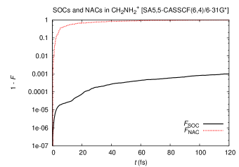
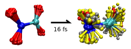
Figure 2: Importance of the SOCs and NACs in the dynamics starting on the second excited electronic state of CH₂NH₂⁺ evaluated with the MSDR combined with the FSSH dynamics. Top: Fast decay of $F_{\text{NAC}}$ signifies the importance of NACs, whereas a very slow decay of $F_{\text{SOC}}$ shows that SOCs may be safely neglected. Bottom: Swarm of 72 trajectories representing the wave packet during the photoisomerization dynamics of CH₂NH₂⁺ immediately after excitation and $\sim 16$ $\mathrm{fs}$ after excitation. Configurations on the first, second, and third lowest-energy excited states are depicted with yellow, red, and pink hydrogen atoms, respectively. Configurations on the ground state have grey hydrogens.

III.3 On-the-fly ab initio collision of F + H₂

The collision of F + H₂ represents a system where SOCs are known to be important at least at low energies.Lique et al. (2008, 2011) In order to check the ability of the MSDR to detect the importance of SOCs, we have applied it together with on-the-fly computed electronic structure using the SA3-CASSCF(9,10)/6-31+G* method. The (9,10) active space was chosen because it is known to produce qualitatively correct smooth PESs for any orientation of H₂ axis.Bauschlicher et al. (1989) The time step of the FSSH dynamics was equal to $\sim 0.2$ $\mathrm{fs}$. Six lowest-energy doublet states were considered in the simulation (three states with $M_{S}=1/2$ and three states with $M_{S}=-1/2$). The initial state was placed either on the electronic ground state or on the first excited state with $M_{S}=1/2$ in the basis diabatic with respect to SOCs and adiabatic with respect to couplings originating in the Born-Oppenheimer separation of motion of electrons and nuclei. (The degeneracy of p states of F was removed by H₂ at a distance of $\sim 6$ Å.) The molecule of H₂ was in the vibrational and rotational ground state with uniformly random orientation of the molecular axis. Translational degrees of freedom of F and H₂ were sampled from GWPs with the mean total kinetic energy of the collision $E_{k}=0.7$ $\mathrm{kcal/mol}$. At such a low energy, both considered collisions were nonreactive.

As can be seen in Fig. 3, fidelity due to SOCs decays significantly in both cases. Relatively fast decay of fidelity in the case of electronically excited initial state signifies importance of SOCs on the collision dynamics. In the case of the ground state collision, fidelity decays more slowly and SOCs may probably be neglected in less accurate simulations. Nevertheless, the decay is sufficient to justify inclusion of SOCs in accurate quantitative simulations. On the other hand, the decay of fidelity due to NACs is similar for both states. For the ground-state dynamics, NACs are comparable in importance to SOCs, whereas for the excited state dynamics, SOCs are clearly much more important.

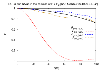
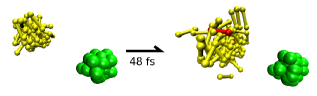
Figure 3: Importance of SOCs and NACs in the collision of F + H₂ evaluated with the MSDR combined with the FSSH dynamics. Top: The decays of $F_{\text{grnd\_SOC}}$ and $F_{\text{exc\_SOC}}$ signify the importance of SOCs, especially in the collision initiated on the first excited electronic state. NACs for both excited and ground state dynamics are as important as SOCs for the ground state dynamics. Bottom: Swarm of 64 trajectories representing the wave packet (initially located on the first excited PES) during the collision of F + H₂ at $t=0$ $\mathrm{fs}$ and $t\sim 48$ $\mathrm{fs}$. Configurations on the first and second lowest-energy excited doublet states are depicted with yellow and red hydrogen atoms, respectively. Configurations on the ground state have grey hydrogens.

IV Conclusions

We have demonstrated that the fidelity criterion may detect disturbances of the quantum dynamics due to SOCs, which may not be found if cruder criteria, such as the extent of the population transfer between PESs, are used. This observation is in accordance with our previous findings on the nondiabaticity and nonadiabaticity of quantum dynamics.Zimmermann and Vaníček (2010, 2012) It should be noted that fidelity is a nonspecific criterion and more specific measures may be constructed when needed in order to attribute the effect of couplings to either the electronic or nuclear dynamics. This can be done, for example, by combination of the fidelity criterion and surface population criterion. However, the separation of the nuclear and electronic effects is not always possible. Fidelity is a rigorous single measure that can take into account both effects simultaneously.

We found that the MSDR approximation of quantum fidelity remains accurate when the perturbation is caused by SOCs. Based on our previous experience, the MSDR may fail, especially in cases where the underlying mixed quantum-classical dynamics does not approximate the quantum dynamics reasonably well. This can happen, e.g., when tunneling is important in the dynamics of the unperturbed Hamiltonian $\mathbf{\hat{H}}^{0}$. In that case, any implementation of the MSDR, which is based on the mixed quantum-classical dynamics, may not work. Other failures are specific to current implementations of MSDR, where both the LMFD and FSSH dynamics may be inaccurate due to the fact that all matrix elements of the density matrix are attached to the same trajectory and evolve on the same PES. A typical situation where approximations of this kind fail occurs when regions of strong coupling are encountered repeatedly and dynamics on PESs between these encounters differ substantially. Surprisingly, in many cases the MSDR stays accurate despite the failure of the underlying dynamics. This is due to the cancellation of errors between the dynamics of $\mathbf{\hat{H}}^{0}$ and the (not explicitly performed) dynamics of $\mathbf{\hat{H}}^{\epsilon}$.

Applications of the MSDR to the photoisomerization dynamics of CH₂NH₂⁺ and to the collision of F + H₂ demonstrated that our method may be used as a tool to decide which PESs and couplings are important in the quantum dynamics, without the need to run quantum dynamics itself. In contrast to the quantum dynamics, the MSDR does not scale exponentially with the number of degrees of freedom, it may be used on the fly and it does not require costly scans of PESs or any other substantial prior knowledge of a system. (Note that there exist several methods of quantum dynamics which may also be used on the fly.Curchod et al. (2011); Wyatt et al. (2001); Lopreore and Wyatt (2002) Nevertheless, they are not currently widely used.) Finally, the MSDR is simple and its current formulations may be very easily implemented into any code for FSSH or Ehrenfest dynamics.

Acknowledgement

This research was supported by the Swiss NSF NCCR MUST (Molecular Ultrafast Science & Technology), Grant No. $200021\_124936/1$, and by the EPFL.

References

- Child and Robb (2004) M. S. Child and M. A. Robb, eds., Non-Adiabatic Effects in Chemical Dynamics, vol. 127 of Faraday Discussions (Royal Society fo Chemistry, Cambridge, UK, 2004).
- Worth and Cederbaum (2004) G. A. Worth and L. S. Cederbaum, Annu. Rev. Phys. Chem. 55, 127 (2004).
- Martinez (2010) T. J. Martinez, Nature 467, 412 (2010).
- Butler (1998) L. J. Butler, Annu. Rev. Phys. Chem. 49, 125 (1998).
- Wu (2010) E. L. Wu, J. Comput. Chem. 31, 2827 (2010).
- Marian (2012) C. M. Marian, Wiley Interdisciplinary Reviews: Computational Molecular Science 2, 187 (2012).
- González-Luque et al. (2010) R. González-Luque, T. Climent, I. González-Ramírez, M. Merchín, and L. Serrano-Andrés, J. Chem. Theory Comput. 6, 2103 (2010).
- Neiss and Saalfrank (2003) C. Neiss and P. Saalfrank, Photochem. Photobiol. 77, 101 (2003).
- Griesbeck et al. (2004) A. G. Griesbeck, M. Abe, and S. Bondock, Acc. Chem. Res. 37, 919 (2004).
- Abe et al. (2004) M. Abe, T. Kawakami, S. Ohata, K. Nozaki, and M. Nojima, J. Am. Chem. Soc. 126, 2838 (2004).
- Maiti et al. (2004) B. Maiti, G. C. Schatz, and G. Lendvay, J. Phys. Chem. A 108, 8772 (2004).
- Lique et al. (2011) F. Lique, G. Li, H.-J. Werner, and M. H. Alexander, J. Chem. Phys. 134, 231101 (2011).
- Takezaki et al. (1998) M. Takezaki, N. Hirota, and M. Terazima, J. Chem. Phys. 108, 4685 (1998).
- Satzger et al. (2004) H. Satzger, B. Schmidt, C. Root, W. Zinth, B. Fierz, F. Krieger, T. Kiefhaber, and P. Gilch, J. Phys. Chem. A 108, 10072 (2004).
- Reichardt et al. (2009) C. Reichardt, R. A. Vogt, and C. E. Crespo-Hernandez, J. Chem. Phys. 131, 224518 (2009).
- Minns et al. (2010) R. S. Minns, D. S. N. Parker, T. J. Penfold, G. A. Worth, and H. H. Fielding, Phys. Chem. Chem. Phys. 12, 15607 (2010).
- Peres (1984) A. Peres, Phys. Rev. A 30, 1610 (1984).
- Zimmermann and Vaníček (2010) T. Zimmermann and J. Vaníček, J. Chem. Phys. 132, 241101 (2010).
- MacKenzie et al. (2012) R. MacKenzie, M. Pineault, and L. Renaud-Desjardins, Can. J. Phys. 90, 187 (2012).
- Zimmermann and Vaníček (2012) T. Zimmermann and J. Vaníček, J. Chem. Phys. 136, 094106 (2012).
- Richter et al. (2011) M. Richter, P. Marquetand, J. González-Vázquez, I. Sola, and L. González, J. Chem. Theory Comput. 7, 1253 (2011).
- Vaníček and Heller (2003) J. Vaníček and E. J. Heller, Phys. Rev. E 68, 056208 (2003).
- Vaníček (2004) J. Vaníček, Phys. Rev. E 70, 055201 (2004).
- Vaníček (2006) J. Vaníček, Phys. Rev. E 73, 046204 (2006).
- Shi and Geva (2004) Q. Shi and E. Geva, J. Chem. Phys. 121, 3393 (2004).
- Miller and Smith (1978) W. H. Miller and F. T. Smith, Phys. Rev. A 17, 939 (1978).
- Hubbard and Miller (1983) L. M. Hubbard and W. H. Miller, J. Chem. Phys. 78, 1801 (1983).
- Mukamel (1982) S. Mukamel, J. Chem. Phys. 77, 173 (1982).
- Gorin et al. (2006) T. Gorin, T. Prosen, T. H. Seligman, and M. Znidaric, Physics Reports 435, 33 (2006).
- Wisniacki et al. (2010) D. A. Wisniacki, N. Ares, and E. G. Vergini, Phys. Rev. Lett. 104, 254101 (2010).
- García-Mata et al. (2011) I. García-Mata, R. O. Vallejos, and D. A. Wisniacki, New J. Phys. 13, 103040 (2011).
- Rost (1995) J. M. Rost, J. Phys. B 28, L601 (1995).
- Li et al. (1996) Z. Li, J.-Y. Fang, and C. C. Martens, J. Chem. Phys. 104, 6919 (1996).
- Egorov et al. (1998) S. A. Egorov, E. Rabani, and B. J. Berne, J. Chem. Phys. 108, 1407 (1998).
- Shi and Geva (2005) Q. Shi and E. Geva, J. Chem. Phys. 122, 064506 (2005).
- Wehrle et al. (2011) M. Wehrle, M. Šulc, and J. Vaníček, Chimia 65, 334 (2011).
- Šulc and Vaníček (2012) M. Šulc and J. Vaníček, Mol. Phys. (2012), URL http://www.tandfonline.com/doi/abs/10.1080/00268976.2012.6689%71.
- Mollica and Vaníček (2011) C. Mollica and J. Vaníček, Phys. Rev. Lett. 107, 214101 (2011).
- Meyer et al. (2009) H.-D. Meyer, F. Gatti, and G. A. Worth, eds., Multidimensional Quantum Dynamics: MCTDH Theory and Applications (Wiley-VCH, Weinheim, 2009).
- Worth et al. (2008) G. A. Worth, H.-D. Meyer, H. Köppel, L. S. Cederbaum, and I. Burghardt, Int. Rev. Phys. Chem. 27, 569 (2008).
- Burghardt et al. (2008) I. Burghardt, K. Giri, and G. A. Worth, J. Chem. Phys. 129, 174104 (2008).
- Blancafort et al. (2011) L. Blancafort, F. Gatti, and H.-D. Meyer, The Journal of Chemical Physics 135, 134303 (2011).
- Martínez et al. (1996) T. J. Martínez, M. Ben-Nun, and R. D. Levine, J. Phys. Chem. 100, 7884 (1996).
- Yang et al. (2009) S. Yang, J. D. Coe, B. Kaduk, and T. J. Martínez, J. Chem. Phys. 130, 134113 (2009).
- Burant and Batista (2002) J. C. Burant and V. S. Batista, J. Chem. Phys. 116, 2748 (2002).
- Kondorskiy and Nakamura (2004) A. Kondorskiy and H. Nakamura, J. Chem. Phys. 120, 8937 (2004).
- Wu and Herman (2005) Y. Wu and M. F. Herman, J. Chem. Phys. 123, 144106 (2005).
- Sun and Miller (1997) X. Sun and W. H. Miller, J. Chem. Phys. 106, 6346 (1997).
- Miller (2009) W. H. Miller, J. Phys. Chem. A 113, 1405 (2009).
- Heller et al. (2002) E. J. Heller, B. Segev, and A. V. Sergeev, J. Phys. Chem. B 106, 8471 (2002).
- Ceotto et al. (2009) M. Ceotto, S. Atahan, G. F. Tantardini, and A. Aspuru-Guzik, J. Chem. Phys. 130, 234113 (2009).
- Tully (1990) J. C. Tully, J. Chem. Phys. 93, 1061 (1990).
- Nielsen et al. (2000) S. Nielsen, R. Kapral, and G. Ciccotti, J. Stat. Phys. 101, 225 (2000).
- Shenvi (2009) N. Shenvi, J. Chem. Phys. 130, 124117 (2009).
- Donoso and Martens (1998) A. Donoso and C. C. Martens, J. Phys. Chem. A 102, 4291 (1998).
- Kapral and Ciccotti (1999) R. Kapral and G. Ciccotti, J. Chem. Phys. 110, 8919 (1999).
- Horenko et al. (2002) I. Horenko, C. Salzmann, B. Schmidt, and C. Schütte, J. Chem. Phys. 117, 11075 (2002).
- Ando and Santer (2003) K. Ando and M. Santer, J. Chem. Phys. 118, 10399 (2003).
- Horenko et al. (2004) I. Horenko, M. Weiser, B. Schmidt, and C. Schütte, J. Chem. Phys. 120, 8913 (2004).
- Micha and Thorndyke (2004) D. A. Micha and B. Thorndyke, in A Tribute Volume in Honor of Professor Osvaldo Goscinski, edited by J. R. Sabin and E. Brandas (Academic Press, 2004), vol. 47 of Advances in Quantum Chemistry, pp. 293 – 314.
- Mac Kernan et al. (2008) D. Mac Kernan, G. Ciccotti, and R. Kapral, J. Phys. Chem. B 112, 424 (2008).
- Bonella et al. (2010) S. Bonella, G. Ciccotti, and R. Kapral, Chem. Phys. Lett. 484, 399 (2010).
- Bousquet et al. (2011) D. Bousquet, K. H. Hughes, D. A. Micha, and I. Burghardt, J. Chem. Phys. 134, 064116 (2011).
- Dunkel et al. (2008) E. R. Dunkel, S. Bonella, and D. F. Coker, J. Chem. Phys. 129, 114106 (2008).
- Huo and Coker (2011) P. Huo and D. F. Coker, J. Chem. Phys. 135, 201101 (2011).
- Berning et al. (2000) A. Berning, M. Schweizer, H.-J. Werner, P. J. Knowles, and P. Palmieri, Mol. Phys. 98, 1823 (2000).
- Wigner (1932) E. Wigner, Phys. Rev. 40, 749 (1932).
- Aleksandrov (1981) I. V. Aleksandrov, Zeitschrift Fur Naturforschung Section A-a Journal of Physical Sciences 36, 902 (1981).
- Boucher and Traschen (1988) W. Boucher and J. Traschen, Phys. Rev. D 37, 3522 (1988).
- Martens and Fang (1997) C. C. Martens and J. Y. Fang, J. Chem. Phys. 106, 4918 (1997).
- Prezhdo and Kisil (1997) O. V. Prezhdo and V. V. Kisil, Phys. Rev. A 56, 162 (1997).
- Caro and Salcedo (1999) J. Caro and L. L. Salcedo, Phys. Rev. A 60, 842 (1999).
- Feit and Fleck (1983) M. D. Feit and J. A. Fleck, Jr., J. Chem. Phys. 78, 301 (1983).
- Verlet (1967) L. Verlet, Phys. Rev. 159, 98 (1967).
- Werner et al. (2010) H.-J. Werner, P. J. Knowles, G. Knizia, F. R. Manby, M. Schütz, P. Celani, T. Korona, R. Lindh, A. Mitrushenkov, G. Rauhut, et al., Molpro, version 2010.1, a package of ab initio programs (2010).
- Lischka et al. (2010) H. Lischka, R. Shepard, I. Shavitt, R. M. Pitzer, M. Dallos, T. Müller, P. G. Szalay, F. B. Brown, R. Ahlrichs, H. J. Böhm, et al., Columbus release 5.9.2, an ab initio electronic structure program (2010).
- Donchi et al. (1988) K. F. Donchi, B. A. Rumpf, G. D. Willett, J. R. Christie, and P. J. Derrick, J. Am. Chem. Soc. 110, 347 (1988).
- Barbatti et al. (2006) M. Barbatti, A. J. A. Aquino, and H. Lischka, Mol. Phys. 104, 1053 (2006).
- Barbatti et al. (2007) M. Barbatti, G. Granucci, M. Persico, M. Ruckenbauer, M. Vazdar, M. Eckert-Maksic̀, and H. Lischka, J. Photochem. Photobiol. A-Chem. 190, 228 (2007).
- Lique et al. (2008) F. Lique, M. H. Alexander, G. Li, H.-J. Werner, S. A. Nizkorodov, W. W. Harper, and D. J. Nesbitt, J. Chem. Phys. 128, 084313 (2008).
- Bauschlicher et al. (1989) J. Bauschlicher, Charles W., S. R. Langhoff, T. J. Lee, and P. R. Taylor, J. Chem. Phys. 90, 4296 (1989).
- Curchod et al. (2011) B. F. E. Curchod, I. Tavernelli, and U. Rothlisberger, Phys. Chem. Chem. Phys. 13, 3231 (2011).
- Wyatt et al. (2001) R. E. Wyatt, C. L. Lopreore, and G. Parlant, J. Chem. Phys. 114, 5113 (2001).
- Lopreore and Wyatt (2002) C. L. Lopreore and R. E. Wyatt, J. Chem. Phys. 116, 1228 (2002).