Optimized Multichannel Quantum Defect Theory for cold molecular collisions

Abstract

Multichannel quantum defect theory (MQDT) can provide an efficient alternative to full coupled-channel calculations for low-energy molecular collisions. However, the efficiency relies on interpolation of the $\bm{Y}$ matrix that encapsulates the short-range dynamics, and there are poles in $\bm{Y}$ that may prevent interpolation over the range of energies of interest for cold molecular collisions. We show how the phases of the MQDT reference functions may be chosen so as to remove such poles from the vicinity of a reference energy and dramatically increase the range of interpolation. For the test case of Mg+NH, the resulting optimized $\bm{Y}$ matrix may be interpolated smoothly over an energy range of several Kelvin and a magnetic field range of over 1000 G. Calculations at additional energies and fields can then be performed at a computational cost that is proportional to the number of channels $N$ and not to $N^{3}$.

I Introduction

Samples of cold and ultracold molecules have unique properties that are likely to have applications in many diverse areas. These include high-precision measurement Hudson et al. (2002); Bethlem and Ubachs (2009), quantum information processing DeMille (2002) and quantum simulation Carr et al. (2009). There is also great interest in the development of controlled ultracold chemistry Krems (2008).

Atomic and molecular interactions and collisions are crucial to the production and properties of cold and ultracold molecules. However, quantum-mechanical molecular collision calculations can be computationally extremely expensive. Such calculations are usually carried out using the coupled-channel method, in which the wavefunction is expanded

$$\Psi(r,\tau)=r^{-1}\sum_{i=1}^{N}\varphi_{i}(\tau)\psi_{i}(r).$$ (1)

Here the $N$ functions $\varphi_{i}(\tau)$ form a basis set for the motion in all coordinates, $\tau$, except the intermolecular distance, $r$, and $\psi_{i}(r)$ is the radial wavefunction in channel $i$. Substituting this expansion into the time-independent Schrödinger equation and projecting onto the basis function $\varphi_{j}(\tau)$ yields a set of $N$ coupled differential equations. The properties of completed collisions are describe by the scattering matrix $\bm{S}$, which is obtained by matching the functions $\psi_{i}(r)$ to free-particle wavefunctions (Ricatti-Bessel functions) at long range Johnson (1973). In the full coupled-channel method, explicit solution of the coupled equations takes a time proportional to $N^{3}$.

The problems encountered in cold molecular collisions often require very large number of channels. Atom-molecule and molecule-molecule interaction potentials can be strongly anisotropic, requiring large basis sets of rotational functions for convergence. In addition, calculations are often required in an applied field, where the total angular momentum $J$ is no longer a good quantum number. Because of this, the large sets of coupled equations cannot be factorized into smaller blocks for each $J$ as is possible in field-free scattering Arthurs and Dalgarno (1960). Furthermore, at the very low collision energies of interest, small splittings between molecular energy levels have important consequences. Effects such as tunneling Żuchowski and Hutson (2009) and nuclear hyperfine splitting Lara et al. (2007); González-Martínez and Hutson (2011) each multiply the number of channels.

In cold collision studies, the scattering $\bm{S}$ matrix is often a fast function of collision energy $E$ and magnetic field $B$, with extensive structure due to scattering resonances and discontinuous behavior at threshold. Calculations are often required over a fine grid of energies and/or applied electric and magnetic fields, and this further multiplies the computational expense.

We have recently shown Croft et al. (2011) that Multichannel Quantum Defect Theory (MQDT) Seaton (1966, 1983); Greene et al. (1982); Mies and Julienne (1984); Mies and Raoult (2000); Raoult and Mies (2004) provides an attractive alternative to full coupled-channel calculations in these circumstances. MQDT attempts to represent the scattering properties in terms of a matrix $\bm{Y}(E,B)$ Greene et al. (1982); Mies and Julienne (1984); Mies and Raoult (2000); Raoult and Mies (2004) that is a smooth function of $E$ and $B$. If this can be achieved, the matrix can be obtained once and then used for calculations over a wide range of energies and fields, or obtained by interpolation from a few points. Once the matrix $\bm{Y}(E,B)$ has been obtained, the time required for calculations at additional energies and fields is only proportional to $N$, not $N^{3}$.

One problem with MQDT is that the $\bm{Y}$ matrix may have poles as a function of $E$ and $B$, and these limit the range over which it can be interpolated. In cold molecular collision studies, calculations are typically needed over an energy range of order 1 K above threshold, and for magnetic fields up to a few thousand gauss . This contrasts with the situation for collisions of ultracold atoms, where the energy range of interest is commonly a few $\mu$K and the fields are typically a few hundred gauss.

In the present paper, we show how MQDT $\bm{Y}$ matrices can be defined to allow smooth interpolation over substantial ranges of collision energy and applied field. This will allow the use of MQDT to provide substantial savings in computer time.

II Theory

A full description of MQDT has been given previously Seaton (1966, 1983); Greene et al. (1982); Mies and Julienne (1984); Mies and Raoult (2000); Raoult and Mies (2004). We give here only a brief description, following ref. Croft et al. (2011), which is sufficient to describe the notation we use.

MQDT defines the matrix $\bm{Y}(E,B)$ at a matching distance $r_{\rm match}$ at relatively short range. The $N$-channel scattering problem at energy $E$ is partitioned into $N_{\rm o}$ open channels (with $E_{i}^{\infty}\leq E$, where $E_{i}^{\infty}$ is the threshold of channel $i$), $N_{\rm c}$ weakly closed channels, and $N_{\rm s}$ strongly closed channels. Strongly closed channels are those that make no significant contribution to the scattering dynamics at $r>r_{\rm match}$.

The scattering dynamics beyond $r_{\rm match}$ is accounted for using single-channel (uncoupled) calculations in a basis set that diagonalizes the Hamiltonian at $r=\infty$. The solution of the multichannel Schrödinger equation at $r>r_{\rm match}$ is written in the matrix form

$$\bm{\Psi}=\bm{f}(r)+\bm{g}(r)\bm{Y},$$ (2)

where $\bm{f}$ and $\bm{g}$ are diagonal matrices containing the functions $f_{i}$ and $g_{i}$, which are linearly independent solutions of a reference Schrödinger equation in each asymptotic channel $i$,

$$\left[-\frac{\hbar^{2}}{2\mu}\frac{d^{2}}{dr^{2}}+U_{i}^{\rm ref}(r)-E\right]f_{i}(r)=0,$$ (3)

and similarly for $g_{i}(r)$. The reference potentials $U_{i}^{\rm ref}(r)$ approach the true potential at long range, and $\mu$ is the reduced mass. They include the centrifugal terms $\hbar^{2}L_{i}(L_{i}+1)/2\mu r^{2}$, where $L_{i}$ is the partial-wave quantum number for channel $i$. $\bm{Y}$ is an $N_{\rm{ref}}\times N_{\rm{ref}}$ matrix, where $N_{\rm{ref}}=N_{\rm o}+N_{\rm c}$.

In our approach Croft et al. (2011), $\bm{Y}$ is obtained numerically by matching the solutions of the coupled-channel equations to $f_{i}(r)$ and $g_{i}(r)$ at $r_{\rm match}$. The $\bm{S}$ matrix is then obtained from $\bm{Y}$ using Eqs. (21) to (23) of ref. Croft et al. (2011), which require 3 QDT parameters $C_{i}$, $\tan\lambda_{i}$ and $\xi_{i}$ in each open channel and a single QDT parameter $\tan\nu_{i}$ in each weakly closed channel. In the open channels the reference functions are asymptotically related to Ricatti-Bessel functions $J_{L_{i}}(r)$ and $N_{L_{i}}(r)$ Johnson (1973),

$$\begin{pmatrix}f_{i}\\ g_{i}\end{pmatrix}=\left(\begin{array}[]{cc}C_{i}&0\\ -C_{i}\tan\lambda_{i}&C_{i}^{-1}\end{array}\right)\left(\begin{array}[]{rr}\cos\xi_{i}&\sin\xi_{i}\\ -\sin\xi_{i}&\cos\xi_{i}\end{array}\right)\begin{pmatrix}J_{L_{i}}\\ N_{L_{i}}\end{pmatrix}.$$ (4)

Here $\xi_{i}$ is the asymptotic phase shift of the function $f_{i}$ with respect to the Ricatti-Bessel function $J_{L_{i}}$. The QDT parameter $C_{i}$ relates the amplitudes of the energy-normalized functions at long range to functions with Wentzel-Kramers-Brillouin (WKB) normalization at short range, while $\tan\lambda_{i}$ describes the modification of the WKB phase due to threshold effects. Far from threshold, $C_{i}\approx 1$ and $\tan\lambda_{i}\approx 0$. In the weakly closed channels the reference functions are asymptotically

$$\begin{pmatrix}f_{i}\\ g_{i}\end{pmatrix}=\left(\begin{array}[]{rr}\cos\nu_{i}&\sin\nu_{i}\\ -\sin\nu_{i}&\cos\nu_{i}\end{array}\right)\begin{pmatrix}\phi_{i}\\ \gamma_{i}\end{pmatrix},$$ (5)

where $\phi_{i}$ is the solution of (3) that decays exponentially at large $r$ and $\gamma_{i}$ is its linearly independent partner, which is exponentially growing.

The absolute phases chosen for the reference functions $f_{i}$ and $g_{i}$ are arbitrary, and different choices produce different $\bm{Y}$ matrices and different MQDT parameters. In particular, Eq. (2) shows that a pole in $\bm{Y}$ occurs whenever the propagated multichannel wavefunction in any channel $i$ has no contribution from the reference function $f_{i}$. However, all phase choices produce the same physical $\bm{S}$ matrix. We are therefore free to choose the phase in order to produce a $\bm{Y}$ matrix with advantageous characteristics. Here we show how the phase may be chosen to produce a $\bm{Y}$ matrix that is pole-free over a wide range of energy or magnetic field and can be interpolated smoothly.

Rotating the reference functions $f_{i}$ and $g_{i}$ by an angle $\theta_{i}$ gives a new set of linearly independent reference functions $\bar{f}_{i}$ and $\bar{g}_{i}$,

$$\begin{pmatrix}\bar{f}_{i}\\ \bar{g}_{i}\end{pmatrix}=\left(\begin{array}[]{rr}\cos\theta_{i}&-\sin\theta_{i}\\ \sin\theta_{i}&\cos\theta_{i}\end{array}\right)\begin{pmatrix}f_{i}\\ g_{i}\end{pmatrix}.$$ (6)

These rotated reference functions define a new $\bm{Y}$ matrix and a new set of QDT parameters ($\bar{C}$, $\tan\bar{\lambda}$, $\bar{\xi}$ and $\tan\bar{\nu}$). Combining equations (4), (5) and (6) gives

$$\bar{\xi}_{i}=\arctan\left[\frac{C_{i}^{2}\sin\xi_{i}(\cos\theta_{i}+\tan\lambda_{i}\sin\theta_{i})-\cos\xi_{i}\sin\theta_{i}}{C_{i}^{2}\cos\xi_{i}(\cos\theta_{i}+\tan\lambda_{i}\sin\theta_{i})+\sin\xi_{i}\sin\theta_{i}}\right],$$ (7)

$$\tan\bar{\lambda}_{i}=-\frac{2C^{4}_{i}\tan\lambda_{i}\cos 2\theta_{i}+\left[1+C^{4}_{i}\left(\tan^{2}\lambda_{i}-1\right)\right]\sin 2\theta_{i}}{2\left(C^{4}_{i}\cos^{2}\theta_{i}+\sin\theta_{i}\left[\sin\theta_{i}+C^{4}_{i}\tan\lambda_{i}(2\cos\theta_{i}+\tan\lambda_{i}\sin\theta_{i})\right]\right)},$$ (8)

$$\bar{C}_{i}=\left(\frac{\sin\xi_{i}\sin\theta_{i}}{C_{i}}+C_{i}\cos\xi_{i}(\cos\theta_{i}+\tan\lambda_{i}\sin\theta_{i})\right)\sqrt{1+\frac{\left(\cos\xi_{i}\sin\theta_{i}-C_{i}^{2}\sin\xi_{i}(\cos\theta_{i}+\tan\lambda_{i}\sin\theta_{i})\right)^{2}}{\left(\sin\xi_{i}\sin\theta_{i}+C_{i}^{2}\cos\xi_{i}(\cos\theta_{i}+\tan\lambda_{i}\sin\theta_{i})\right)^{2}}},$$ (9)

$$\bar{\nu}_{i}=\nu_{i}-\theta_{i}.$$ (10)

Far from threshold ($E\gg 1$ K), Eqs. (7) to (10) simplify to $\bar{\xi}_{i}=\xi_{i}-\theta_{i}$, $\tan\lambda_{i}\approx 0$, $C_{i}\approx 1$ and $\bar{\nu}_{i}=\nu_{i}-\theta_{i}$. However, in the threshold region that is of interest in cold molecule studies, Eqs. (7) to (10) must be evaluated explicitly.

II.1 Basis sets and quantum numbers

As a test case, we consider cold collisions between NH (${}^{3}\Sigma^{-}$) and Mg atoms Wallis and Hutson (2009). This is the same system as considered in ref. Croft et al. (2011), but the present work uses a larger basis set which introduces more scattering resonances and denser poles in the $\bm{Y}$ matrix.

The energy levels of NH in a magnetic field are most conveniently described using Hund’s case (b), in which the molecular rotation $n$ couples to the spin $s$ to produce a total monomer angular momentum $j$. In zero field, each rotational level $n$ is split into sublevels labeled by $j$. In a magnetic field, each sublevel splits further into $2j+1$ levels labeled by $m_{j}$, the projection of $j$ onto the axis defined by the field. For the $n=0$ levels that are of most interest for cold molecule studies, there is only a single zero-field level with $j=1$ that splits into three components with $m_{j}=+1$, $0$ and $-1$.

The coupled equations are constructed in a partly coupled basis set $|nsjm_{j}\rangle|LM_{L}\rangle$, where $L$ is the end-over-end rotational angular momentum of the Mg atom and the NH molecule about one another and $M_{L}$ is its projection on the axis defined by the magnetic field. Hyperfine structure is neglected. The matrix elements of the total Hamiltonian in this basis set are given in ref. González-Martínez and Hutson (2007). The only good quantum numbers during the collision are the parity $p=(-1)^{n+L+1}$ and the total projection quantum number $M=m_{j}+M_{L}$. The calculations in the present work are performed for $p=-1$ and $M=1$. This choice includes s-wave scattering of NH molecules in initial state $m_{j}=+1$, which is magnetically trappable, to $m_{j}=0$ and $-1$, which are not. The present work uses a converged basis set including all functions up to $n_{\text{max}}=6$ and $L_{\text{max}}=8$, as in ref. Wallis and Hutson (2009).

We label elements of $\bm{Y}$ and $\bm{S}$ by subscripts $\alpha,L,M_{L}\rightarrow\alpha^{\prime},L^{\prime},M_{L}^{\prime}$, where $\alpha$ represents an eigenstate of free NH that may be approximately labeled by $(n,s,j,m_{j})$. However, the collisions considered in the present paper are all among the $n=0,j=1$ levels and so $\alpha$ is simply abbreviated to $m_{j}$. For diagonal elements we suppress the second set of labels.

II.2 Numerical methods

The coupled-channel calculations required for both MQDT and the full coupled-channel approach were carried out using the MOLSCAT package Hutson and Green (1994), as modified to handle collisions in magnetic fields González-Martínez and Hutson (2007). The coupled equations were solved numerically using the hybrid log-derivative propagator of Alexander and Manolopoulos Alexander and Manolopoulos (1987), which uses a fixed-step-size log-derivative propagator in the short-range region ($r_{\text{min}}\leq r<r_{\text{mid}}$) and a variable-step-size Airy propagator in the long-range region ($r_{\text{mid}}\leq r\leq r_{\text{max}}$). The full coupled-channel calculations used $r_{\text{min}}=2.5$ Å, $r_{\text{mid}}=50$ Å and $r_{\text{max}}=250$ Å (where 1 Å = $10^{-10}$ m). MQDT requires coupled-channel calculations only from $r_{\text{min}}$ to $r_{\rm match}$ (which is less than $r_{\text{mid}}$), so only the fixed-step-size propagator was used in this case.

The MQDT reference functions and quantum defect parameters were obtained as described in ref. Croft et al. (2011), using the renormalized Numerov method Johnson (1977) to solve the 1-dimension Schrödinger equations for the reference potentials. The MQDT $\bm{Y}$ matrix was then obtained by matching to the log-derivative matrix extracted from the coupled-channel propagation at a distance $r_{\text{match}}$. In this paper all MQDT calculations use the reference potential

$$U^{\text{ref}}_{i}(r)=V_{0}(r)+\frac{\hbar^{2}L_{i}(L_{i}+1)}{2\mu r^{2}}+E_{i}^{\infty},$$ (11)

where $V_{0}(r)$ is the isotropic part of the interaction potential. This reference potential has been shown to produce quantitatively accurate results when $\bm{Y}$ is reevaluated at each collision energy and magnetic field Croft et al. (2011). However, such reevaluation relinquishes most of the computational savings that MQDT is intended to achieve.

The reference potential contains a hard wall at $r=r^{\text{wall}}_{i}$, so that $U^{\text{ref}}_{i}(r)=\infty$ for $r<r^{\text{wall}}_{i}$. In the present paper we take $r^{\text{wall}}_{i}=4.0$ Å. Figure 1 shows the reference potentials for the lowest three rotational states.

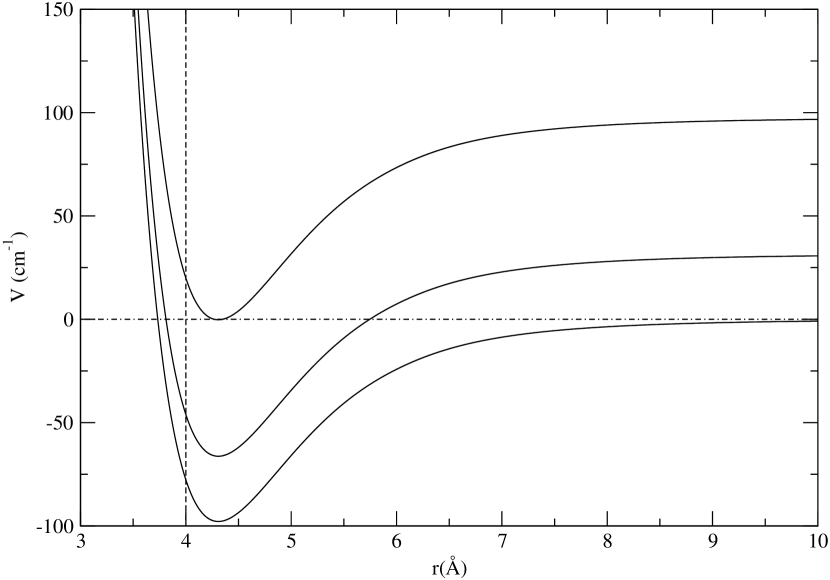
Figure 1: The $V_{0}$ reference potentials for Mg + NH. The first and second rotational excited state are also shown ($n=1,2$). The hard wall at $r=4.0$ Å is shown as a vertical dashed line. The dot-dashed horizontal line corresponds to zero energy.

All channels with $n\geq 2$ were treated as strongly closed and thus not included in the MQDT part of the calculation, but were included in the log-derivative propagation.

III Results and discussion

The top panel of Fig. 2 shows a single diagonal element of the $\bm{Y}$ matrix, $Y_{-1,8+3}$, as a function of the matching distance and energy, obtained with unrotated reference functions. $Y_{-1,8,+3}$ is a representative element of $\bm{Y}$ with poles at the same locations as the other elements, chosen to give a good visual representation of the pole structure. There are many poles visible, which prevent polynomial interpolation over energies of more that 0.5 K for any value of $r_{\rm match}$ (and much less than this for some choices of $r_{\rm match}$). The energies of the poles become independent of $r_{\rm match}$ at long range.

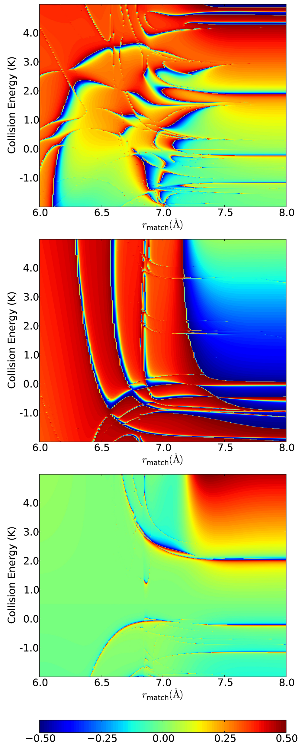
Figure 2: (Color online) Contour plot of $\arctan Y_{ii}/\pi$ for a representative diagonal $\bm{Y}$ matrix element, $Y_{-1,8,+2}$, as a function of energy and $r_{\text{match}}$ at $B=10$ G. Top panel: obtained with unrotated reference functions ($\theta_{i}=0$). Center panel: obtained with reference functions rotated by $\theta_{i}=\pi/2$. Bottom panel: obtained with optimized reference functions with $\theta_{i}=\theta_{i}^{\rm{opt}}$ in all channels. The arctangent is show for clarity of plotting: it maps the real numbers, $\mathbb{R}$, to the domain $-\pi/2$ to $\pi/2$, thus allowing all magnitudes of $\bm{Y}$ matrix elements to be seen on a single plot.

The presence of low-energy poles in $\bm{Y}$ for some values of $r_{\rm match}$ is a serious problem. For MQDT to be efficient, $r_{\rm match}$ must be chosen without solving the coupled equations at many different energies. The calculations needed to produce contour plots such as those in Fig. 2 are feasible for a test case such as Mg+NH, but would be prohibitively expensive for a very large system.

The center panel of Fig. 2 shows the same element of the $\bm{Y}$ matrix as a function of the matching distance and energy for reference functions rotated by $\theta_{i}=\pi/2$. The poles are in quite different places, but once again there are many of them. The combination of the top and center panels demonstrates that, for any arbitrary choice of rotation angle, poles will appear in the $\bm{Y}$ matrix, preventing simple interpolation for most choices of $r_{\rm match}$. This will be true in any MQDT problem with a large density of resonances. The contour plots do however show that the position of poles is strongly dependent on the rotation angle, even at large values of $r_{\rm match}$. This suggests that it will be possible to optimize the rotation angle in order to move the poles away from the energy range of interest. It is emphasized that the $\bm{S}$ matrices obtained from the $\bm{Y}$ matrices shown in the different panels of Fig. 2 are identical.

We now consider how to rotate the reference functions to maximize the pole-free range over which $\bm{Y}$ can be interpolated. $Y_{ii}$ as a function of $\theta_{i}$ is given by

$$Y_{ii}=\tan(\theta_{i}+\delta_{i}),$$ (12)

where $\delta_{i}$ is the phase shift between the unrotated reference function $f_{i}$ and the propagated multichannel wavefunction in channel $i$. There is a pole in $Y_{ii}$ when $\theta_{i}+\delta_{i}=\pi$ and a zero when $\theta_{i}+\delta_{i}=0$. We thus set $\theta_{i}^{\rm opt}=-\delta_{i}$ at one choice of $r_{\rm match}$, $E$ and $B$, so that the propagated multichannel wavefunction and the reference wavefunctions are almost in phase and the resulting $\bm{Y}$ matrix in that region is pole-free.

Because the channels are coupled, rotating the reference functions in one channel affects the other elements of the $\bm{Y}$ matrix. In this work we loop over the channels sequentially, setting each diagonal element to 0 in turn. By repeatedly looping over all channels, all the diagonal $\bm{Y}$ matrix elements are set to 0. For Mg+NH it was sufficient to loop over the channels twice. In a more strongly coupled system it is expected that this would need to be repeated more times. This approach allows a set of optimized $\theta_{i}$ to be obtained from a single multichannel propagation.

Rotated reference functions have previously been used to transform $\bm{Y}$ matrices in the study of atomic spectra Giusti-Suzor and Fano (1984a, b, c); Cooke and Cromer (1985); Eissner et al. (1969) and atomic collisions Osséni et al. (2009). Adjusting $\theta_{i}$ at each energy such that $Y_{ii}=0$ was shown to produce a weak energy dependence of off-diagonal $\bm{Y}$ matrix elements across thresholds Osséni et al. (2009). However, this approach required propagating the full multichannel wavefunction many times at different energies, which is precisely what the present work tries to avoid.

The bottom panel of Fig. 2 shows how the representative element $Y_{-1,8,+2}^{\rm opt}$ varies as a function of the matching distance and energy. All the $\theta_{i}$ values are optimized as described above at $E=0.5$ K and $B=10$ G for each value of $r_{\rm match}$, but are not reoptimised at each energy. Comparison of this with the upper two panels shows the effectiveness of optimizing the reference functions. Without optimization, there were no choices of $r_{\rm match}$ for which $\bm{Y}$ was pole-free and thus suitable for interpolation over the energy range of interest. After optimization, $\bm{Y}^{\rm opt}$ is pole-free over a substantial range, of about 1 K, for any choice of $r_{\rm match}<8$ Å. For values of $r_{\rm match}<6.5$ Å, $\bm{Y}^{\rm opt}$ is pole-free over many Kelvin. Beyond 6.5 Å, poles start to enter $\bm{Y}^{\rm opt}$ in the energy range of interest. Once the poles have settled at their asymptotic values at $r_{\rm match}>7.5$ Å, we find that positive energies up to about 2 K are pole-free. However, at larger values of $r_{\rm match}$ the linearity of $\bm{Y}^{\rm opt}$ over the pole-free region decreases. This is due to negative energy poles in the $\bm{Y}$ matrix which our procedure cannot move significantly. There is one particularly bad choice of $r_{\rm match}$ at $\approx 6.8$ Å, but provided this unlucky choice of $r_{\rm match}$ is avoided, $\bm{Y}^{\rm opt}$ can be interpolated smoothly over the positive energy range from 0 to $>2$ K for any choice of $r_{\rm match}$.

Figure 3 compares diagonal T-matrix elements $|T_{ii}|^{2}$ (where $T_{ij}=\delta_{ij}-S_{ij}$) obtained from full coupled-channel calculations with those from the MQDT method, with a matching distance of $r_{\text{match}}=6.5$ Å, using reference functions optimized at 0.5 K. MQDT results were obtained both by recalculating the $\bm{Y}$ matrix at every energy and by interpolating $\bm{Y}^{\rm opt}$ linearly between two points separated by 1 K. The MQDT results with $\bm{Y}$ recalculated at each energy can scarcely be distinguished from the full coupled-channel results. The MQDT results obtained by interpolation are also very similar to the full coupled-channel results except around the resonance feature at $E\approx 0.1$ K. The interpolated result could of course be improved simply by performing coupled-channel calculations to obtain $\bm{Y}^{\rm opt}$ at one or two extra energies across the range, to allow for a higher-order interpolation, or by using a linear interpolation over a smaller energy range.

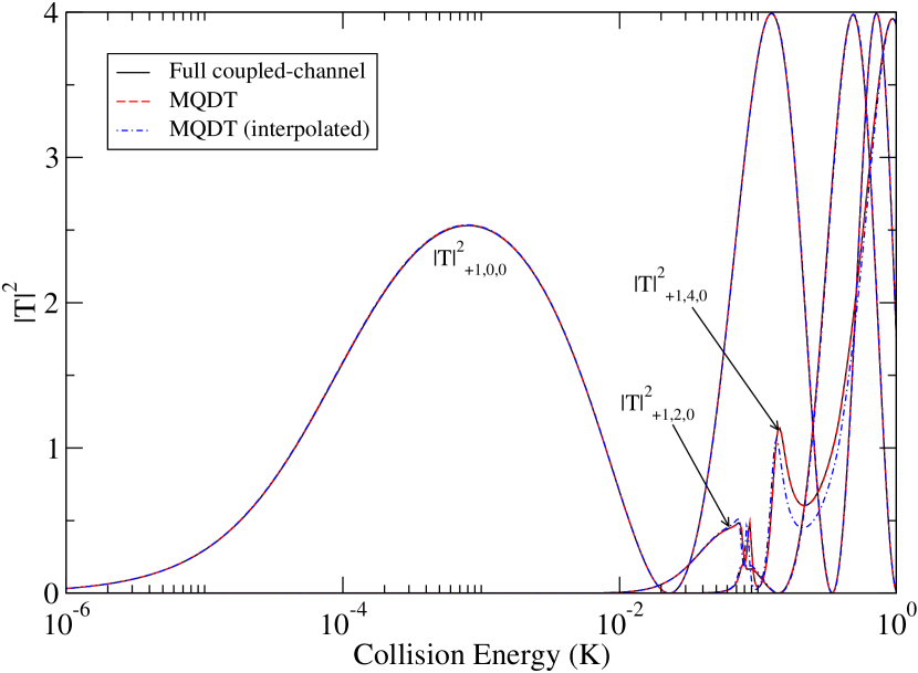
Figure 3: (Color online) The squares of diagonal T-matrix elements $T_{m_{j},L,M_{L}}$ in the incoming channels for $m_{j}=+1$ and $L=0$, 2 and 4 at $B=10$ G, obtained from full coupled-channel calculations (solid, black) and MQDT with optimized reference functions for $r_{\rm match}$ = 6.5 Å, both with (dot-dash, blue) and without (dashed, red) interpolation.

In this work we use $\theta_{i}$ to rotate our short-range reference functions $f_{i}$ and $g_{i}$. In principle, we could rotate the reference functions by varying the asymptotic phase shifts $\xi_{i}$ instead of the short-range phases $\theta_{i}$. However Figure 4 shows why this is not desirable.

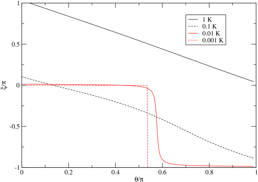
Figure 4: (Colour online) The asymptotic phase shift $\bar{\xi}_{i}$ as a function of the rotation angle $\theta$ for the incoming d-wave channel ($+1,2,0$).

Due to the highly nonlinear relationship between $\xi_{i}$ and $\theta_{i}$, obtaining the optimum rotation angle of the short-range reference functions $f_{i}$ and $g_{i}$ by varying the angle $\xi_{i}$ would be laborious at very low collision energies.

III.1 Magnetically tunable Feshbach resonances

The effects of magnetic fields on cold molecular collisions are very important, since collisions can be controlled by taking advantage of magnetically tunable low-energy Feshbach resonances. We are therefore interested in how $\bm{S}$ matrix elements behave as a function of magnetic field across Feshbach resonances. It is thus important that the $\bm{Y}$ matrix is weakly dependent on magnetic field in such regions.

Figure 5 shows the diagonal elements of the optimized $\bm{Y}$ matrix as a function of magnetic field for Mg + NH collisions over the range from 10 G to 5000 G for a collision energy of 1 mK. This range of fields tunes across 6 Feshbach resonances. The reference functions were optimized at 10 G and 1 mK. The elements of $\bm{Y}^{\rm opt}$ are smoothly curved over the entire 5000 G range and could be well represented by a low-order polynomial.

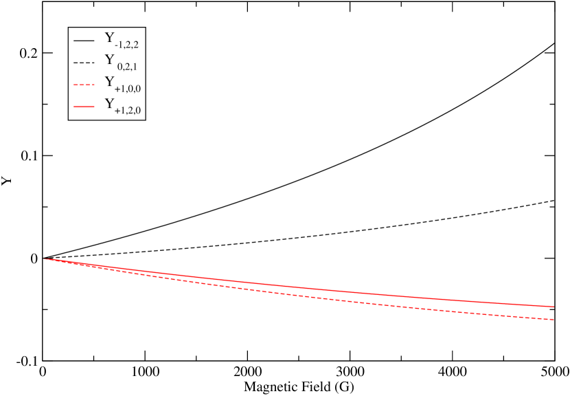
Figure 5: (Color online) Representative $\bm{Y}^{\rm{opt}}$ matrix elements as a function of field at $E=1$ mK.

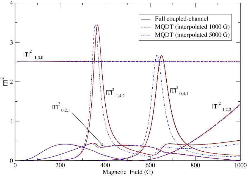
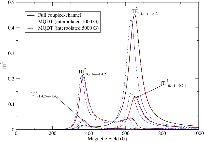
Figure 6: (Color online) Squares of T-matrix elements at 1 mK as a function of field in the vicinity of a Feshbach resonance. Upper panel: diagonal elements; lower panel: off-diagonal elements.

Figure 6 shows the comparison between optimized MQDT and full coupled-channel calculations for a selection of diagonal and off-diagonal T-matrix elements as the magnetic field is tuned at 1 mK. The reference functions were optimized at 10 G and 1 mK and MQDT results were obtained by linear interpolation of $\bm{Y}^{\rm opt}$ between two points separated by 1000 G and by 5000 G. Interpolation over 1000 G gives resonance features that are in very good agreement with the full coupled-channel calculation to better than 1 G. Interpolation over 5000 G gives resonance features of the correct shape, with positions that are still within about 10 G of the full coupled-channel results. The difference between the interpolated result and the full coupled-channel calculation is a result of both the choice of $r_{\rm match}$ and the interpolation. The quality of the interpolation could be improved by considering a few more fields across the range to allow for higher-order polynomial interpolation or by using linear interpolation over a smaller field range.

Full MQDT calculations recalculating the $\bm{Y}$ matrix at every magnetic field give resonance positions accurate to 0.4 G. The remaining errors between the full coupled-channel calculations and the MQDT results will reduce with a larger choice of $r_{\rm match}$. As seen in the bottom panel of Fig. 2, the optimized $\bm{Y}$ matrices obtained at larger values of $r_{\rm match}$ are still amenable to interpolation, though over a more restricted energy range.

IV Conclusions

We have shown that Multichannel Quantum Defect Theory can provide an efficient computational method for low-energy molecular collisions as a function of both energy and magnetic field. In particular, we have shown how a disposable parameter of MQDT, the phase of the short-range reference functions, may be chosen to make the MQDT $\bm{Y}$ matrix smooth and pole-free over a wide range of energy and field. This smooth variation allows the $\bm{Y}$ matrix to be evaluated from coupled-channel calculations at a few values of the energy and field and then to be obtained by interpolation at intermediate values. It is not necessary to repeat the expensive coupled-channel part of the calculation on a fine grid.

The procedure developed here is to choose the phase of the reference functions in each channel so that the diagonal $\bm{Y}$ matrix in each channel is zero at a reference energy and field. This ensures that there are no poles in the $\bm{Y}$ matrix, which would prevent smooth interpolation, close to the reference energy. Optimizing the phase in this way is very inexpensive, and once it is done the cost of calculations at additional energies and fields varies only linearly with the number of channels $N$, not as $N^{3}$ as for full coupled-channel calculations. MQDT with optimized $\bm{Y}$ matrices is thus a very promising alternative to full coupled-channel calculations for cold molecular collisions, particularly when fine scans over collision energy and magnetic field are required.

The $\bm{Y}$ matrix is defined to encapsulate all the collision dynamics that occurs inside a matching distance $r_{\rm match}$, and the choice of this distance is important. There is a trade-off between the accuracy of the method and the size of the pole-free region of the optimized $\bm{Y}$ matrix. For large values of $r_{\rm match}$, resonant features may appear in the $\bm{Y}$ matrix and prevent simple interpolation over large ranges of energy and field. For smaller values of $r_{\rm match}$, optimizing the reference functions allows interpolation over many Kelvin, but the accuracy of MQDT is reduced because interchannel coupling is neglected outside $r_{\rm match}$.

For the moderately anisotropic Mg + NH system studied here, optimized MQDT with an interpolated $\bm{Y}$ matrix can provide numerical results in quantitative agreement with fully converged coupled-channel calculations. In future work, we will investigate the extension of this approach to more strongly coupled systems, with larger anisotropy of the interaction potential and more closed channels that produce scattering resonances.

V Acknowledgments

JFEC is grateful to EPSRC for a High-End Computing Studentship. The authors are grateful for support from EPSRC, AFOSR MURI Grant FA9550-09-1-0617, and EOARD Grant FA8655-10-1-3033

References

- Hudson et al. (2002) J. J. Hudson, B. E. Sauer, M. R. Tarbutt, and E. A. Hinds, Phys. Rev. Lett. 89, 023003 (2002).
- Bethlem and Ubachs (2009) H. L. Bethlem and W. Ubachs, Faraday Discuss. 142, 25 (2009).
- DeMille (2002) D. DeMille, Phys. Rev. Lett. 88, 067901 (2002).
- Carr et al. (2009) L. D. Carr, D. DeMille, R. V. Krems, and J. Ye, New J. Phys. 11, 055049 (2009).
- Krems (2008) R. V. Krems, Phys. Chem. Chem. Phys. 10, 4079 (2008).
- Johnson (1973) B. R. Johnson, J. Comput. Phys. 13, 445 (1973).
- Arthurs and Dalgarno (1960) A. M. Arthurs and A. Dalgarno, Proc. Roy. Soc., Ser. A 256, 540 (1960).
- Żuchowski and Hutson (2009) P. S. Żuchowski and J. M. Hutson, Phys. Rev. A 79, 062708 (2009).
- Lara et al. (2007) M. Lara, J. L. Bohn, D. E. Potter, P. Soldán, and J. M. Hutson, Phys. Rev. A 75, 012704 (2007).
- González-Martínez and Hutson (2011) M. L. González-Martínez and J. M. Hutson, Phys. Rev. A 84, 052706 (2011).
- Croft et al. (2011) J. F. E. Croft, A. O. G. Wallis, J. M. Hutson, and P. S. Julienne, Phys. Rev. A 84, 042703 (2011).
- Seaton (1966) M. J. Seaton, Proc. Phys. Soc. 88, 801 (1966).
- Seaton (1983) M. J. Seaton, Rep. Prog. Phys. 46, 167 (1983).
- Greene et al. (1982) C. H. Greene, A. R. P. Rau, and U. Fano, Phys. Rev. A 26, 2441 (1982).
- Mies and Julienne (1984) F. H. Mies and P. S. Julienne, J. Chem. Phys. 80, 2526 (1984).
- Mies and Raoult (2000) F. H. Mies and M. Raoult, Phys. Rev. A 62, 012708 (2000).
- Raoult and Mies (2004) M. Raoult and F. H. Mies, Phys. Rev. A 70, 012710 (2004).
- Note (1) Units of gauss rather than tesla, the accepted SI unit of magnetic field, are used in this paper to conform to the conventional usage of this field.
- Wallis and Hutson (2009) A. O. G. Wallis and J. M. Hutson, Phys. Rev. Lett. 103, 183201 (2009).
- González-Martínez and Hutson (2007) M. L. González-Martínez and J. M. Hutson, Phys. Rev. A 75, 022702 (2007).
- Hutson and Green (1994) J. M. Hutson and S. Green, “MOLSCAT computer program, version 14,” distributed by Collaborative Computational Project No. 6 of the UK Engineering and Physical Sciences Research Council (1994).
- Alexander and Manolopoulos (1987) M. H. Alexander and D. E. Manolopoulos, J. Chem. Phys. 86, 2044 (1987).
- Johnson (1977) B. R. Johnson, J. Chem. Phys. 67, 4086 (1977).
- Giusti-Suzor and Fano (1984a) A. Giusti-Suzor and U. Fano, J. Phys. B 17, 215 (1984a).
- Giusti-Suzor and Fano (1984b) A. Giusti-Suzor and U. Fano, J. Phys. B 17, 4267 (1984b).
- Giusti-Suzor and Fano (1984c) A. Giusti-Suzor and U. Fano, J. Phys. B 17, 4277 (1984c).
- Cooke and Cromer (1985) W. E. Cooke and C. L. Cromer, Phys. Rev. A 32 (1985).
- Eissner et al. (1969) W. Eissner, H. Nussbaumer, H. E. Saraph, and M. J. Seaton, J. Phys. B 2, 341 (1969).
- Osséni et al. (2009) R. Osséni, O. Dulieu, and M. Raoult, J. Phys. B 42, 185202 (2009).