Endocortical bone loss in osteoporosis:
The role of bone surface availability

Abstract --

Age-related bone loss and postmenopausal osteoporosis are disorders of bone remodelling, in which less bone is reformed than resorbed. Yet, this dysregulation of bone remodelling does not occur equally in all bone regions. Loss of bone is more pronounced near and at the endocortex, leading to cortical wall thinning and medullary cavity expansion, a process sometimes referred to as “trabecularisation” or “cancellisation”. Cortical wall thinning is of primary concern in osteoporosis due to the strong deterioration of bone mechanical properties that it is associated with. In this paper, we examine the possibility that the non-uniformity of microscopic bone surface availability could explain the non-uniformity of bone loss in osteoporosis. We use a computational model of bone remodelling in which microscopic bone surface availability influences bone turnover rate and simulate the evolution of the bone volume fraction profile across the midshaft of a long bone. We find that bone loss is accelerated near the endocortical wall where the specific surface is highest. Over time, this leads to a substantial reduction of cortical wall thickness from the endosteum. The associated expansion of the medullary cavity can be made to match experimentally observed cross-sectional data from the Melbourne Femur Collection. Finally, we calculate the redistribution of the mechanical stresses in this evolving bone structure and show that mechanical load becomes critically transferred to the periosteal cortical bone.

Key words: osteoporosis, endocortical bone loss, cortical thinning, specific surface, mathematical modelling

1 Introduction

It is well known that cortical porosity of bone increases in osteoporosis leading to a reduction in bone stiffness and strength, ultimately increasing the risk of fracture [1, 2, 3, 4, 5, 6, 7]. The temporal evolution of this deterioration process in single individuals is still poorly understood. Most of our current knowledge is deduced from cross-sectional data collected by micro-computed tomography of bones. These data indicate that changes in cortical porosity are not uniformly distributed across the cortical thickness. In particular, in long bones, loss is more pronounced near the endocortical surface [2, 5, 6, 7, 3, 1, 4, 8]. Age-related bone loss is therefore characterized by an expansion of the marrow (or medullary) cavity. The result of this process is often referred to as “trabecularisation” of cortical bone, since the aged cortical bone exhibits morphological similarities with trabecular bone [8]. In the following, we refer to this non-uniform bone loss of cortical bone as endocortical bone loss. Endocortical bone loss results in a reduction in cortical wall thickness and in an increase in porosity which consequently reduces the load-bearing capacity of bone [4].

Several mechanisms have been hypothesised to drive bone loss in osteoporosis, including hormonal changes, reduced physical activity, and an evolving bone micro-structure leading to changes in bone surface availability. Hormonal changes are associated with increased remodelling activity, reduction in osteoblast activity, reduction in osteoblast number, and bone imbalance within single basic multicellular units (BMUs) [9, 4, 10]. To explain the non-uniformity of age-related bone loss, RB Martin suggested that bone loss may be influenced by the microscopic availability of bone surface [11, 12]. Based on experimental data, Martin demonstrated a remarkable relationship between bone porosity and bone specific surface (i.e., surface area per volume of bone tissue). Using this relationship, Martin found from a simple mathematical model that in cortical bone increased resorption activity of bone cells would lead to an increase in surface area which in turn would lead to an acceleration in resorption activity, hence, creating a morphological (or geometrical) feedback [11]. In trabecular bone this situation is reversed: increased resorption activity would lead to a decrease in surface area which in turn would lead to a reduction in resorption activity. Martin’s hypothesis that bone remodelling in osteoporosis contains such a morphological feedback by the evolving bone micro-structure is difficult to study experimentally and Martin did not provide any comparison to experimental data. Indeed, the time scales involved in osteoporosis are large, and there is no easy experimental control of the strength of the morphological feedback, nor of how bone morphology changes with age.

In this paper we propose a computational modelling approach suited to the investigation of the non-uniformity of bone loss in osteoporosis attributed to a morphological regulation. Changes in cortical bone volume fraction occurring in the midshaft of human femur bone are evolved numerically assuming an initial bone state and an osteoporotic condition. Our computational model follows Martin’s idea [11, 12]: we hypothesise that the experimentally observed non-uniform loss of bone in osteoporosis (e.g., more pronounced near and at the endocortex) is due to the superposition of:

• Hormonal changes and/or changes in the overall loading, leading to a uniform baseline of bone loss across the cortical bone;

• An evolving bone microstructure, that locally increases or decreases bone remodelling activity (by morphological feedback), and so locally increases or decreases bone loss compared to the hormonal/mechanical baseline.

Our main hypothesis is that the above mechanisms are able to explain (at least in part) the rate of endocortical bone loss represented by the expansion of the medullary cavity, for which there are experimental data available [2]. The predominant loss of bone in the endocortical region is expected to increasingly transfer mechanical loading towards the periosteum.

To test these hypotheses we extend the (purely temporal) mathematical model initially proposed by Martin [12] to include a spatial component. The resulting spatio-temporal description enables us to follow the evolution of the distribution of bone volume fraction across the midshaft of a long bone. The feedback of bone morphology on the bone cells is implemented using the phenomenological relationship between bone porosity and bone specific surface mentioned above. Furthermore, we investigate changes in the distribution of mechanical stresses across the midshaft attributable to the evolving bone microstructure. The distribution of the mechanical stresses is calculated using an extension of classical beam theory to materials of non-uniform composition. This theory and the mathematical model of bone remodelling are presented in Section 2. The numerical results are shown in Section 3 and discussed in Section 4.

2 Methods

In this section, we first present a mathematical model of bone remodelling well-suited to investigate the role of non-uniform bone surface availability for endocortical bone loss such as that which occurs leading to osteoporosis. We then present the method by which the redistribution of the internal mechanical stresses will be calculated when bone has evolving non-uniform properties.

Computational model of bone remodelling including morphological regulation

Bone remodelling is a complex metabolic process that involves regulations at several time scales and length scales. To follow the evolution of bone properties that are relevant to the macroscopic degradation of bone in osteoporosis, we consider a computational model focused on a millimetre-size tissue scale (see Figure 1a). This observation scale is large enough for local resorption and formation processes to be of macroscopic significance for the mechanical and microstructural properties of the tissue [13, 14], and yet small enough for the cellular origin of resorption and formation to be considered with biochemical and morphological regulations [15, 16]. At the tissue scale, the various cell populations involved in bone remodelling can be represented by continuous variables, i.e. local cell densities $n({\boldsymbol{r}},t)$, by means of local averages over a so-called ‘representative volume element’ (RVE) of the tissue $\text{$V_{\text{T}}$}\approx 3\text{--}8\ ^{3}$:

$$n({\boldsymbol{r}},t)\equiv\frac{N({\boldsymbol{r}},t)}{\text{$V_{\text{T}}$}},$$ (1)

where $N({\boldsymbol{r}},t)$ is the number of cells in the volume $V_{\text{T}}$ centred at position ${\boldsymbol{r}}$, at time $t$ (see Figure 1a).

(a)	(b)

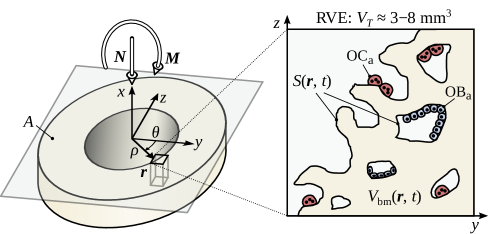
Figure 1: (a) Compressive force ${\boldsymbol{N}}$ and bending moment ${\boldsymbol{M}}$ acting in a cross-section (of area $A$) of a long bone. The representative volume element (RVE) of the tissue at position ${\boldsymbol{r}}$ serves to define local spatial averages of bone properties, such as cell densities, bone matrix volume fraction $f_{\text{bm}}$ and specific surface $s_{V}$. (b) Relationship between specific surface $s_{V}$ and bone matrix volume fraction $f_{\text{bm}}$ as in Eq. (7) (redrawn from Ref. [12]).

Stiffness properties of a millimetre-size portion of bone tissue are determined to a great extent by the bone volume fraction (or equivalently the bone porosity) and the elastic properties of the mineralised bone matrix [13, 14]. In osteoporosis, both bone volume fraction and the overall degree of mineralisation of bone matrix are decreased. Osteoporosis is associated with increased remodelling activity with net bone loss per remodelling event that becomes progressively stronger with time [4]. This rapid remodelling both exacerbates bone loss and replaces more densely mineralised matrix with younger, less mineralised matrix [17]. In this paper, we focus on age-related changes in the morphological rather than mineral properties of the bone tissue. Such morphological changes have been studied extensively in cadaver bone specimens from the Melbourne Femur Collection [2, 5, 6, 7]. Changes in the degree of mineralisation of bone matrix will be considered in future studies. The bone volume fraction $\text{$f_{\text{bm}}$}({\boldsymbol{r}},t)$ of a portion of bone tissue represents the relative amount of bone matrix (volume $V_{\text{bm}}$) in the RVE of volume $V_{T}$:

$$\text{$f_{\text{bm}}$}({\boldsymbol{r}},t)\equiv\frac{V_{\text{bm}}({\boldsymbol{r}},t)}{\text{$V_{\text{T}}$}}.$$ (2)

Local bone matrix is continually renewed by remodelling. In homeostasis, resorption and formation are balanced and remodelling leads to bone turnover without loss or gain. In osteoporosis, less bone is reformed than is resorbed, so bone turnover is associated with a net bone loss. The evolution of the local bone volume fraction $f_{\text{bm}}$ is governed by (i) the local densities of active osteoblasts (OB${}_{\text{a}}$) and active osteoclasts (OC${}_{\text{a}}$) and (ii) these cells’ activity rates:

$$\tfrac{\partial}{\partial t}\text{$f_{\text{bm}}$}({\boldsymbol{r}},t)=\text{$k_{\text{form}}$}\text{{OB}${}_{\text{a}}$}({\boldsymbol{r}},t)-\text{$k_{\text{res}}$}\text{{OC}${}_{\text{a}}$}({\boldsymbol{r}},t),$$ (3)

where $k_{\text{form}}$ is the volume of new bone synthesised per unit time by a single active osteoblast and $k_{\text{res}}$ the volume of bone resorbed per unit time by a single active osteoclast.

Equation (3) expresses generally the balance between bone formation and bone resorption: $k_{\text{form}}$OB${}_{\text{a}}$ corresponds to the formation rate (bone volume fraction synthesised per unit time) and $k_{\text{res}}$OC${}_{\text{a}}$ corresponds to the resorption rate (bone volume fraction resorbed per unit time). The difficulty in Eq. (3) lies in determining the evolution of the populations of active osteoclasts and active osteoblasts, and in particular, in determining how their densities depend themselves on the presence of bone matrix. Osteoclasts and osteoblasts usually require a pre-existing bone substrate to conduct their resorbing and synthesising activities. The densities of osteoclasts and osteoblasts thus depend on the local amount of bone surface (area $S$) available to them in the RVE, i.e., on the specific surface $\text{$s_{V}$}({\boldsymbol{r}},t)$:

$$\text{$s_{V}$}({\boldsymbol{r}},t)\equiv\frac{S({\boldsymbol{r}},t)}{\text{$V_{\text{T}}$}}.$$ (4)

Comprehensive cell population models of osteoblasts and osteoclasts including biochemical coupling have been proposed in the literature [21, 22, 15, 23, 24, 25]. In Ref. [25], the potential influence of the specific surface $s_{V}$ on various stages of osteoblast and osteoclast developments is investigated in the bone cell population model of Refs [15, 24]. Here, however, we will consider a simpler model of bone cells, originally formulated by Martin [12]. The advantage of this simpler model is that the dependence upon $s_{V}$ of the densities of active osteoclasts and active osteoblasts appears explicitly. Whilst full biochemical coupling between cells is not explicit in this model, the non-uniformity and evolution of the bone surface availability are accounted for, which are important to capture non-uniform effects of remodelling during age-related bone loss according to our hypotheses.

Bone tissues with a large specific surface exhibit more remodelling, and so contain more active osteoblasts and active osteoblasts, than tissues with a small specific surface (Figure 1a) [12]. Denoting by $\lambda_{\text{{OB}${}_{\text{a}}$}}$ and $\lambda_{\text{{OC}${}_{\text{a}}$}}$ the fractions of the bone surface at which there is osteoblastic and osteoclastic activity due to remodelling, and by $\sigma_{\text{{OB}${}_{\text{a}}$}}$ and $\sigma_{\text{{OC}${}_{\text{a}}$}}$ the surface densities of active osteoblasts and active osteoclasts at remodelling sites, the densities of active osteoblasts and active osteoclasts are given by $\text{{OB}${}_{\text{a}}$}=\lambda_{\text{{OB}${}_{\text{a}}$}}\sigma_{\text{{OB}${}_{\text{a}}$}}\text{$s_{V}$}$ and $\text{{OC}${}_{\text{a}}$}=\lambda_{\text{{OC}${}_{\text{a}}$}}\sigma_{\text{{OC}${}_{\text{a}}$}}\text{$s_{V}$}$. Substituting these expressions in Eq. (3), one thus has [12]:

$$\tfrac{\partial}{\partial t}\text{$f_{\text{bm}}$}({\boldsymbol{r}},t)=\big{(}\text{$k_{\text{form}}$}\lambda_{\text{{OB}${}_{\text{a}}$}}\sigma_{\text{{OB}${}_{\text{a}}$}}-\text{$k_{\text{res}}$}\lambda_{\text{{OC}${}_{\text{a}}$}}\sigma_{\text{{OC}${}_{\text{a}}$}}\big{)}\ \text{$s_{V}$}({\boldsymbol{r}},t).$$ (5)

Whilst Eq. (5) holds generally, in the following, it is assumed that $k_{\text{form}}$, $k_{\text{res}}$, $\lambda_{\text{{OB}${}_{\text{a}}$}}$, $\lambda_{\text{{OC}${}_{\text{a}}$}}$, $\sigma_{\text{{OB}${}_{\text{a}}$}}$, $\sigma_{\text{{OC}${}_{\text{a}}$}}$ can be taken uniform and constant in time. This is clearly a simplification, as the microscopic availability of bone surface may influence the recruitment and development of bone cells in a nontrivial way. These recruitment and development processes determine the fractions $\lambda_{\text{{OB}${}_{\text{a}}$}}$ and $\lambda_{\text{{OC}${}_{\text{a}}$}}$, which would thus normally be expected to depend additionally on $s_{V}$ [25]. Here, a simple extensivity of cell densities in $s_{V}$ is assumed when taking OB${}_{\text{a}}$ and OC${}_{\text{a}}$ just proportional to $s_{V}$.

In osteoporosis, a net bone loss is associated with each remodelling event. To retrieve physiological overall rates of bone loss, Martin assumed a small imbalance between formation and resorption, setting [12]:

$$\text{$k_{\text{form}}$}\lambda_{\text{{OB}${}_{\text{a}}$}}\sigma_{\text{{OB}${}_{\text{a}}$}}-\text{$k_{\text{res}}$}\lambda_{\text{{OC}${}_{\text{a}}$}}\sigma_{\text{{OC}${}_{\text{a}}$}}=-2\ \micro\text{/year}.$$ (6)

This constant baseline of bone loss means that a 2 $\micro$-thick layer of bone matrix is resorbed each year on all bone surfaces. This baseline of bone loss is weighted by the specific surface to correspond to volumetric losses in the local RVE of the tissue $V_{\text{T}}$.

Bone tissues exhibit a wide range of microstructures each characterising a particular volume fraction and specific surface. Cortical bone typically has volume fractions $\text{$f_{\text{bm}}$}\approx 0.85\text{--}0.95$ with pores mainly constituted of Haversian canals. Trabecular bone typically has volume fractions $\text{$f_{\text{bm}}$}\approx 0.15\text{--}0.55$ with ‘pores’ corresponding to the marrow space around the trabecular plates and struts. Based on measurements performed in a large variety of bone tissues, Martin [12] has proposed that bone volume fraction $f_{\text{bm}}$ and specific surface $s_{V}$ follow an ‘intrinsic’ or ‘universal’ relationship, approximated by the following polynomial:

$$\text{$s_{V}$}(\text{$f_{\text{bm}}$})=a_{1}\text{$f_{\text{bm}}$}+a_{2}\text{$f_{\text{bm}}$}^{2}+a_{3}\text{$f_{\text{bm}}$}^{3}+a_{4}\text{$f_{\text{bm}}$}^{4}+a_{5}\text{$f_{\text{bm}}$}^{5},$$ (7)

with

$$a_{1}=14.1/,\ \ a_{2}=-10.5/,\ \ a_{3}=-17.8/,$$

$$a_{4}=43.0/,\ \ a_{5}=-28.8/.$$ (8)

The relation (7) is plotted in Figure 1b together with experimental data assembled in Ref. [12] from various types of human bones (femur, iliac crest, vertebra, rib) both in health and disease. Importantly, the specific surface exhibits a maximum $\text{$s_{V}$}^{\star}\approx 4.2/$ at a bone volume fraction $\text{$f_{\text{bm}}$}^{\ast}\approx 0.63$, intermediate between cortical and trabecular bone.

Using the phenomenological relation (7) and Eq. (6) in Eq. (5), one is able to calculate the evolution of bone volume fraction $\text{$f_{\text{bm}}$}({\boldsymbol{r}},t)$ in every region ${\boldsymbol{r}}$ of the bone tissue, given an initial distribution of bone volume fraction $\text{$f_{\text{bm}}$}({\boldsymbol{r}},t_{0})$. This evolution enables us to determine how the medullary cavity expands in time for comparison with experimental data [2]. It is well-known that the distinction between cortical and trabecular bone is not straightforward in osteoporosis [8]. Similarly, measuring the extent of the medullary cavity relies on a visual or morphological threshold to define the endocortical surface. For the purpose of this paper, we assume that the medullary cavity is defined by the region of bone tissue in which bone volume fraction is lower than a threshold $\text{$f_{\text{bm}}$}^{\ast}$. We will take this threshold as the bone volume fraction at which the specific surface is maximum according to Eq. (7), i.e. $\text{$f_{\text{bm}}$}^{\ast}\approx 0.63$. The effect of choosing different threshold values for the determination of medullary cavity radius will also be investigated (see Figure 2d).

The simplicity of the model considered here (as opposed to more detailed models of bone cell developments such as that of Ref. [25]) has two practical consequences: (i) the specific surface $s_{V}$ enters as an explicit dependence in the right hand side of Eq. (5). This allows the formulation of a semi-analytical solution for the evolution of bone volume fraction $f_{\text{bm}}$ (see Appendix A); (ii) the governing equation for the bone volume fraction is self-contained: the state of the system depends only on the current distribution profile of the bone volume fraction. This enables us to easily regress the system backwards in time and to deduce the past distribution of bone volume fraction that has led to an experimentally observed medullary cavity expansion (see Appendix B).

Internal mechanical stress distribution

Mechanical loading is carried non-uniformly by bone tissues. In particular, the cortex carries the majority of the loads applied to a bone [8]. Here, we consider a long bone subject to a compressive resultant force ${\boldsymbol{N}}(t)=-N(t)\,\hat{{\boldsymbol{x}}}$ along $x$ and a resultant bending moment ${\boldsymbol{M}}(t)=M_{y}(t)\,\hat{{\boldsymbol{y}}}+M_{z}(t)\,\hat{{\boldsymbol{z}}}$ in the cross-sectional ${\boldsymbol{y}}=(y,z)$ plane (see Figure 1a; $\hat{{\boldsymbol{x}}}$, $\hat{{\boldsymbol{y}}}$, and $\hat{{\boldsymbol{z}}}$ denote units vectors along the $x$, $y$, and $z$ axes). To estimate how internal mechanical stresses are redistributing across the midshaft section of a long bone during age-related endocortical bone loss, we use a simple theory of elasticity extended to beams of non-uniform composition (see, e.g., Refs [26, 27, 28]). This theory is based on two main assumptions:

1. Hooke’s law is valid locally at the tissue scale, i.e., the stress tensor $\sigma({\boldsymbol{r}},t)$ and strain tensor $\varepsilon({\boldsymbol{r}},t)$ are related by a local stiffness tensor $E({\boldsymbol{r}},t)$ of the tissue:

   $$\sigma({\boldsymbol{r}},t)=E({\boldsymbol{r}},t)\varepsilon({\boldsymbol{r}},t)$$ (9)

2. Near the midshaft of a long bone, small deformations generated by compression and bending keep the initial cross-sections planar and normal to the neutral axis. This geometrical constraint on the deformations is called the Euler–Bernoulli kinematic hypothesis.

From a structural point of view, long bones near the midshaft can be regarded as weakly deformed long beams. In absence of torsional loads or twisting along the beam axis, as assumed here, the deformation state of such beams is well approximated by the Euler–Bernoulli hypothesis [26, 28, 27]. The Euler–Bernoulli hypothesis implies that the strain tensor $\varepsilon({\boldsymbol{r}},t)$ reduces to the single nonzero scalar component $\varepsilon_{xx}({\boldsymbol{r}},t)$ [28, 27]. For an orthotropic material such as bone [13], this implies by Eq. (9) that there are no shear stresses. The only nonzero components of the stress tensor for such materials are the normal stresses $\sigma_{xx}$, $\sigma_{yy}$ and $\sigma_{zz}$. The normal stresses $\sigma_{yy}$ and $\sigma_{zz}$ are induced by the ‘Poisson effect’ (i.e., thickening of a material under compression) and are usually small except in particular materials such as rubber [28, 27],[29, §17]. The normal stresses $\sigma_{yy}$ and $\sigma_{zz}$ do not participate directly to the transfer of the resultant compressive force ${\boldsymbol{N}}(t)$ and bending moment ${\boldsymbol{M}}(t)$ across the tissue. Indeed, the resultant force ${\boldsymbol{N}}(t)$ and moment ${\boldsymbol{M}}(t)$ are given as integrals of the stress distribution $\sigma_{xx}({\boldsymbol{r}},t)$ in the midshaft cross-section [27, Secs 5.3, 6.2] (see below). For this reason, in the following we will focus on the distribution of normal stresses $\sigma_{xx}({\boldsymbol{r}},t)$ only. From Hooke’s law (9), one has $\sigma_{xx}({\boldsymbol{r}},t)=E_{1111}({\boldsymbol{r}},t)\varepsilon_{xx}({\boldsymbol{r}},t)$, and so only the single component $E_{1111}$ of the stiffness tensor needs to be considered, which corresponds to the compressive stiffness. We will omit any indices for notational simplicity, and write $E_{1111}({\boldsymbol{r}},t)\equiv E({\boldsymbol{r}},t)$.

We consider a cross-section at a position $x$ along the bone axis, near the midshaft, and use the coordinates ${\boldsymbol{y}}\equiv(y,z)$ to denote a position in the cross-sectional plane (see Figure 1a). By definition, the resultant force ${\boldsymbol{N}}(t)$ and resultant moment ${\boldsymbol{M}}(t)$ are given as integrals of the stress distribution $\sigma({\boldsymbol{y}},t)\equiv\sigma_{xx}({\boldsymbol{r}},t)$ in the midshaft cross-section (we omit both the cross-section position ‘$x$’ and the component indices ‘$xx$’ from the notation). With Hooke’s law (9), one thus has [27, Secs 5.3, 6.2]:

$$N(t)=\int_{A}\!\!E({\boldsymbol{y}},t)\,\varepsilon({\boldsymbol{y}},t)\,\mathrm{d}y\mathrm{d}z,$$ (10)

$$M_{y}(t)=-\int_{A}\!\!z\,E({\boldsymbol{y}},t)\,\varepsilon({\boldsymbol{y}},t)\,\mathrm{d}y\mathrm{d}z,$$ (11)

$$M_{z}(t)=\int_{A}\!\!y\,E({\boldsymbol{y}},t)\,\varepsilon({\boldsymbol{y}},t)\,\mathrm{d}y\mathrm{d}z,$$ (12)

where the integrals are carried over the bone cross-sectional area $A$ (Figure 1a). The geometric constraint imposed by the Euler–Bernoulli condition implies that the strain distribution $\varepsilon({\boldsymbol{y}},t)$ is a linear function of the transverse spatial coordinates ${\boldsymbol{y}}=(y,z)$ (see e.g. Ref. [27, Sec. 5.2]):

$$\varepsilon({\boldsymbol{y}},t)\equiv\varepsilon_{1}(t)-\kappa_{3}(t)\,y+\kappa_{2}(t)\,z,$$ (13)

where $\varepsilon_{1}$ is the sectional axial strain, and $\kappa_{2}$ and $\kappa_{3}$ are the sectional beam curvature about the $y$ and $z$ axes, respectively. At each time $t$, the Euler–Bernoulli condition (13) together with the constraints (10)–(12) form a system of three linear equations determining the three unknowns $\varepsilon_{1}(t)$, $\kappa_{2}(t)$ and $\kappa_{3}(t)$. The coefficients of this system of equations involve so-called ‘sectional stiffness coefficients’, i.e., zero order, first order and second order moments of the non-uniform stiffness across the section [27, Sec. 6.2]:

$$S(t)\equiv\int_{A}\!\!\!E({\boldsymbol{y}},t)\,\mathrm{d}y\mathrm{d}z,\quad S_{j}(t)\equiv\int_{A}\!\!\!x_{j}\,E({\boldsymbol{y}},t)\,\mathrm{d}y\mathrm{d}z,$$

$$I_{jk}\equiv\int_{A}\!\!\!x_{j}x_{k}\,E({\boldsymbol{y}},t)\,\mathrm{d}y\mathrm{d}z,\quad i,j=2,3$$ (14)

(with $x_{2}=y$ and $x_{3}=z$). Once $\varepsilon_{1}(t)$, $\kappa_{2}(t)$ and $\kappa_{3}(t)$ are known, the mechanical stress distribution in the cross-section is given by use of Hooke’s law:

$$\sigma({\boldsymbol{y}},t)=E({\boldsymbol{y}},t)\ \big{[}\varepsilon_{1}(t)-\kappa_{3}(t)\,y+\kappa_{2}(t)\,z\big{]}$$ (15)

The sectional stiffness coefficients (14) entering the system of equations to solve are specified at each time $t$ provided the stiffness coefficient $E({\boldsymbol{y}},t)$ is known. Measurements of the compressive stiffness of bone in relation to the amount of bone matrix suggest that stiffness and bone volume fraction are related by a nonlinear phenomenological relationship [30, 31, 20, 32, and Refs cited therein], which we take here as:

$$E({\boldsymbol{y}},t)=E\big{(}\text{$f_{\text{bm}}$}({\boldsymbol{y}},t)\big{)}=C\ \text{$f_{\text{bm}}$}({\boldsymbol{y}},t)^{3},$$ (16)

where $C\approx 15\text{ GPa}$ and $\text{$f_{\text{bm}}$}({\boldsymbol{y}},t)$ is governed by the balance equation (5).

3 Results

Equation (5) determines the evolution of the bone volume fraction $\text{$f_{\text{bm}}$}({\boldsymbol{r}},t)$ at each position ${\boldsymbol{r}}$ within bone from a given initial condition $\text{$f_{\text{bm}}$}({\boldsymbol{r}},t_{0})$. Here for simplicity only rotation-symmetric initial distributions are considered in a cross-section at $x$, implying that $f_{\text{bm}}$ stays rotation-symmetric at all times: $\text{$f_{\text{bm}}$}({\boldsymbol{r}},t)=\text{$f_{\text{bm}}$}(y,z,t)=\text{$f_{\text{bm}}$}(\rho,t)$, where $\rho=\sqrt{y^{2}+z^{2}}$ is the radial coordinate. The initial condition at time $t_{0}$ is assumed to correspond to the bone state at the onset of osteoporosis. The time elapsed since onset of osteoporosis is denoted by $\Delta t_{\text{OP}}\equiv t\!-\!t_{0}$. A constant compressive force $N(t)\equiv 0.4$ kN and constant bending moment around the $z$ axis $M_{z}(t)\equiv 2~{}\text{kN}\cdot\text{m},\,M_{y}(t)\equiv 0$, are assumed when calculating the redistribution of the mechanical stresses. Below, we first show how the bone volume fraction $\text{$f_{\text{bm}}$}(\rho,t)$ evolves by means of Eq. (5) from a typically expected radial profile, and we determine the medullary cavity expansion that this evolution induces (Section 3.1). In a second numerical experiment, we calculate the “inverse problem”, i.e., we use morphological data by Feik et al. [2] compiled into an experimentally observed average medullary cavity expansion in men to determine what initial bone state would have generated this medullary expansion (Section 3.2).

3.1 Evolution of a typical bone volume fraction distribution

(a)	(d)
(b)	(e)
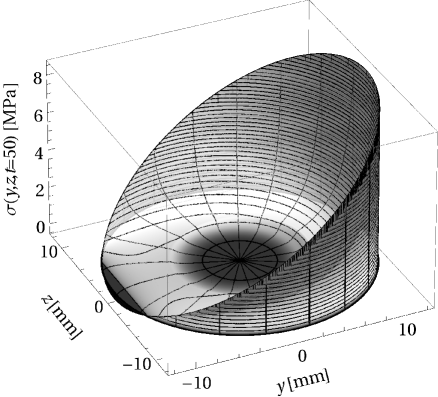
(c)	(f)

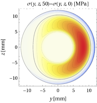
Figure 2: (a)–(c) Calculated radial profiles shown every 10 years since onset of osteoporosis for (a) bone volume fraction; (b) internal stresses at three different polar angles; (c) specific surface. The arrows indicate the evolution of the profiles with osteoporosis; (d) Calculated expansion of the medullary cavity radius. The effect of the threshold used to defined the radius is shown. Thresholds from $\text{$f_{\text{bm}}$}=0.1$ to $\text{$f_{\text{bm}}$}=0.9$ are used (thin solid lines) in addition to the threshold $\text{$f_{\text{bm}}$}=f_{\text{bm}}^{\ast}$ at which $s_{V}$ is maximum (thick solid line). The filled region is indicative of the reduction in cortical wall thickness; (e) Stress distribution across the midshaft cross-section for compression and bending, exhibiting a neutral axis at $y\approx-10\$; (f) Contour plot of the difference in internal stresses between intial bone state and bone state reached after 50 years of osteoporosis. Red tones: decrease in stresses; Blue tones: increase in stresses; Thick grey curve: no change in stresses (zero isoline).

In Figure 2a, the bone volume fraction radial profile $\text{$f_{\text{bm}}$}(\rho,t)$ is shown every 10 years from the onset of osteoporosis ($\Delta t_{\text{OP}}\!=\!0$) for 50 years. The assumed initial bone volume fraction profile at $\Delta t_{\text{OP}}\!=\!0$ (solid line) consists of (i) a sigmoid function of $\rho$ with value zero for $\rho\lesssim 3.3\$ (medullary cavity), sharply increasing (endocortical region) to the value $0.75$ at $\rho\approx 6.3\$ and (ii) a linear function more slowly increasing (intracortical region) to the value $0.99$ from $\rho\approx 6.3\$ to $\rho=12\$ (periosteum, bone radius). Figure 2b and 2c show the corresponding changes in the radial profile of internal stresses $\sigma(\rho,\theta,t)$ and specific surface $\text{$s_{V}$}(\rho,t)$ across the midshaft. In contrast to $f_{\text{bm}}$ and $s_{V}$, the internal stresses $\sigma$ are not rotation-symmetric due to the action of the bending loading condition. The evolution of $\sigma$ is shown at three angles $\theta$ of the polar coordinate system ($\theta=0$,$\tfrac{\pi}{2}$, and $\pi$), where $\theta$ is measured from the $y$ axis (see Figure 1a). The full polar distribution of stresses is shown in Figure 2e at $\Delta t_{\text{OP}}=50$ years.

The bone volume fraction in Figure 2a is seen to decrease in all regions of the bone cross-section due to the simulated osteoporotic condition. However, as expected from Eq. (5), bone loss is more pronounced in the endocortical-to-intracortical region, where the specific surface is high. High bone volume fractions near the periosteum are comparatively more preserved. In the endocortical region, the bone volume fraction profile is both lowered and shifted towards the periosteum by the progression of osteoporosis, resulting overall in a more gradual increase of bone volume fraction from the medullary region to the periosteum than the initial profile.

The radial profile of the specific surface (Figure 2c) gradually evolves such that its maximum originally at $\rho\approx 5.5\$ is shifted towards the periosteum. The position of this maximum corresponds to the intersection between the bone volume fraction and the constant value $\text{$f_{\text{bm}}$}^{\ast}\approx 0.63$ in Figure 2a because $\text{$f_{\text{bm}}$}^{\ast}$ maximises the function $\text{$s_{V}$}(\text{$f_{\text{bm}}$})$ in Eq. (7). Taking $\text{$f_{\text{bm}}$}^{\ast}$ as the threshold value to define the transition between medullary cavity and cortex, this shift of the maximum of the specific surface towards the periosteum corresponds to an expansion of the medullary cavity radius with age. This expansion is plotted separately in Figure 2d (thick solid line). Thin solid lines in Figure 2d correspond to the expansion of a medullary radius defined by other threshold values of $f_{\text{bm}}$ as indicated by the labels. In Figure 2d, the onset of osteoporosis was assumed at 40 years of age. For the threshold value $\text{$f_{\text{bm}}$}^{\ast}$, the increase in medullary radius is initially slow, then accelerates at age $\approx 55$. The cortical wall thickness corresponds to the distance between periosteal bone radius (here assumed fixed at 12 mm) and medullary cavity radius, and is shown by the grey-shaded area. The expansion of the medullary cavity is therefore associated to a thinnning of the cortical wall thickness.

These changes in morphological parameters are associated with a gradual transfer of the internal mechanical stresses towards the periosteum for $\theta=0$ and $\theta=\pi/2$ (Figure 2b), whilst the stress radial profile at $\theta=\pi$ changes little. Interestingly, Figure 2b suggests that for each polar angle $\theta$, there is a well-defined radius below which stresses are decreased and above which stresses are increased. The polar dependence of this radius can be appreciated in Figure 2f. In Figure 2f, isolines of the difference between initial stress distribution and stress distribution after 50 years of osteoporosis are shown. The radius below which stresses are decreased and above which stresses are increased corresponds to the intersection between $\sigma(\rho,\theta,\Delta t_{\text{OP}}\!=\!0)$ and $\sigma(\rho,\theta,\Delta t_{\text{OP}}\!=\!50)$ in Figure 2b, and to the zero isoline in Figure 2f, shown as a thick grey line. The region where stresses are increased is shaded with blue tones and the region where stresses are decreased is shaded with yellow–red tones.

3.2 Determination of past bone volume fraction profile from an observed medullary cavity expansion

As explained in Appendix B, it is possible to use our model to regress the system backwards in time. This can be used to take as input a given medullary cavity expansion and deduce from it the past distribution of bone volume fraction that leads to such an expansion when evolved by the model. Mathematically, this “inverse problem” can only be solved provided the medullary cavity radius is monotonously increasing. Also, the bone volume fraction profile can only be determined between the minimum and the maximum medullary cavity radii of the given expansion. In Figure 3b, we show an observation of medullary cavity expansion obtained by Feik et al. [2] from cross-sectional samples of the Melbourne Femur Collection. In the original data, samples were grouped in decade age categories (such as 31–40 years, 41–50 years etc.) and the medullary area was measured on each sample. Here we have transformed medullary area into medullary radius by assuming a rotation-symmetric medullary cavity and we have interpreted the value in a decade age category as the value at a single age in the timeline (namely, the middle age of the category: 31–40 years $\to$ 35 years). Because the “inverse problem” requires a monotonously increasing radius, we took the data presented in Figure 5 of Ref. [2] for males and discarded the first data point, as indicated by the hatched area in Figure 3b.

(a)	(b)

Figure 3: (a) Determination of bone volume fraction profiles in the endocortical region (non-hatched area) from a given expansion of medullary cavity radius (b). The data in (b) is taken from male bone samples in Ref. [2, Fig. 5]. (The parallel periosteal expansion found in these male bone samples is not considered; a constant periosteal bone radius of 12 mm is assumed here instead.) Only the monotonously increasing part of the curve (non-hatched area) can be used to determine the evolution of bone volume fraction profiles (see Appendix B).

In Figure 3a, we show the bone volume fraction radial profile at 35 years of age (solid line) that reproduces the medullary cavity radius of Figure 3b when evolved to 95 years (double dashed line). As in Figure 2a, the calculated bone volume fraction profile is shown every 10 years and the medullary cavity radius is determined by the intersection of the bone volume fraction profile with the constant value $\text{$f_{\text{bm}}$}^{\ast}$ (dotted horizontal line). In Figure 3b, the minimum radius is $\approx 6.4\$ and the maximum radius is $\approx 9.6\$, and so the bone volume fraction profile in Figure 3a is only determined between these radii as indicated by the excluded hatched areas.

4 Discussion

The study of age-related endocortical bone loss in humans is a challenging problem, with a multitude of possible causes, including biochemical, biomechanical and morphological regulations of bone remodelling. Whilst micro-CT imaging technology can give detailed insights into the bone microstructure at a given moment, to follow the evolution of bone microstructure across a whole cross-section with a degree of detail and a frequency that are sufficiently informative (i) is not currently possible without harmful radiation and (ii) would require several decades of study. Furthermore, soft tissues and bone cells are not seen in micro-CT bone scans. Two different approaches have been undertaken by biologists. Animals models of osteoporosis have been proposed, for which both micro-CT scans and histomorphometric analyses of bone samples can be performed, providing both bone morphological parameters and biochemical information. However, particularly in small animals that lack secondary osteons (such as mice and rats), the pathogenesis of osteoporosis may be quite different from that in humans. In humans, loss of endocortical bone in osteoporosis is believed to progress by expansion and coalescence of Haversian pores near the endosteum [5, 6, 7]. A second approach is to collect cross-sectional data from bone samples (either ex vivo or post mortem) and reconstruct pseudo time sequences by grouping the data by age categories [3, 2, 5, 6, 7]. The advantage of this approach is the direct measurement of human morphological properties of bone. The disadvantage is that measurements can often only be done at a single point in time in an individual.

To our knowledge, there is currently no experimental work specifically studying the influence of the microscopic bone morphology on the development and/or activity of bone cells. Such a morphological feedback on bone remodelling is challenging to investigate experimentally for the following reasons: (i) a morphological feedback cannot be inhibited to estimate its influence (in contrast to biochemical regulations that can be selectively inhibited by gene knock-outs in animal models); (ii) there is no easy control of the bone microstructure in vivo; (iii) in osteoporosis, changes in bone volume fraction occur over long time scales. Computational modelling is a powerful tool that enables the testing of hypotheses for the underlying mechanisms responsible for age-related endocortical bone loss. Most importantly, computational modelling enables the extrapolation of data measured at a single point in time into a predicted evolution over several decades. This is of particular importance for the development of patient-specific assessment and treatment tools for osteoporosis.

The main result of this paper is the observation that a morphological feedback of the bone microstructure (specifically, of the bone specific surface) on the bone cells is able to explain (at least partly) the predominant loss of bone in the endocortical region. The non-uniformity of this loss can develop from a uniform baseline of bone imbalance per remodelling event as caused by systemic hormonal changes or overall changes in mechanical loading due to reduced physical activity. The loss of endocortical bone leads to an expansion of the medullary cavity that is compatible with experimentally observed rates. Furthermore, the deterioration of bone in the endocortical region leads to a transfer of the mechanical stresses towards the periosteum.

The evolution of the radial profile of bone volume fraction in the bone midshaft in Figure 2a is governed by a partial differential equation in time only. However, spatial non-uniformities enter the equation by means of the local availability of bone surface embodied by the specific surface $s_{V}$. Age-related cortical bone loss results in both an overall decrease in cortical bone volume fraction, and a decrease in cortical wall thickness due to pronounced bone loss at the endocortical surface, where the specific surface is high. This is consistent with the experimental findings of Ref. [3].

The precise form of the expansion of the medullary cavity radius shown in Figure 2d depends strongly on the assumed initial bone volume fraction profile and on the threshold value of bone volume fraction used to define the boundary between medullary cavity and cortex. The initial slow increase in medullary radius in Figure 2d is due to the loss of bone in the region $3.3\ \lesssim\rho\lesssim 6\$ (initial endocortical region). In this region, the intial bone volume fraction increases sharply from 0 to 0.75 with the radial coordinate $\rho$, forming a “step” (Figure 2a). Once the sloped “plateau” of bone volume fraction for $\rho\gtrsim 6\$ (initial intracortical region) has reached the threshold bone volume fraction defining the medullary cavity boundary, the expansion of medullary radius increases rapidly in Figure 2d before gradually slowing down due to the relative preservation of bone volume fraction near the periosteum. In fact, choosing a different threshold volume fraction essentially delays or advances this general behaviour. From these results, one can deduce that for the influence of a morphological feedback, the sharper the transition between medullary cavity (zero bone volume fraction) and cortex (high bone volume fraction), the slower the medullary cavity expansion. This observation emphasises the importance of building up “good bones” during growth, with high intracortical volume fractions [37].

We note that an acceleration of the medullary cavity expansion is seen in males between the age groups 81–90 and 91–100 in the data reported in Ref. [2, Fig. 5b] (corresponding to the age interval 85–95 in Figure 3b). This acceleration could be explained by the specific shape of the bone volume fraction radial profile at the onset of osteoporosis. From our model, the bone volume fraction at age 35 shown in Figure 3a, calculated such that it leads to the experimental medullary expansion of Figure 3b, exhibits a similar sharp “step” (associated with a slow medullary expansion) followed by a “sloped plateau” (associated with a fast medullary expansion) as in Figure 2a. However, other physiological factors not accounted for in our model may play a role in this experimentally observed acceleration of the medullary expansion, such as a difference in hormonal imbalance with advancing age that could lead to an increased bone imbalance per remodelling event. We also note that in Figure 5 of Ref. [2], this acceleration of the medullary expansion occurs in parallel to an expansion of the subperiosteal cross-sectional area. Cortical wall thickness decreased in the male bone samples of Ref. [2] between the age groups 61–70 and 81–90 (corresponding to the age interval 65–85 in Figure 3b) due to both an increase in medullary cavity and decrease in subperiosteal cross-sectional area. However, cortical wall thickness was relatively preserved between the age group 81–90 and 91–100 (corresponding to the age interval 85–95 in Figure 3b) as a result of periosteal apposition. In our model, changes in periosteal bone radius are not considered. Whilst bone remodelling processes are observed at the periosteum [38, 4], periosteal apposition is thought to occur via bone modelling processes, which are not well described by our model in its current form.

Figures 2b and 2e clearly show that internal stresses become increasingly and disproportionately redistributed on the strongest part of the bone midshaft, i.e., towards the bone periphery. This disproportionate redistribution could put the bone integrity at increased risk. Indeed, the periosteum is a surface with low remodelling rate [38, 4]. An acceleration of microcrack generation at the periosteum can be expected, increasing the risk of a macroscopic fracture. However, this increased risk may be offset by periosteal bone apposition [2, 39, 4].

Increased stresses towards the periosteum may also account for a conservation of intracortical pore area. In the current model a mechanical feedback to form bone at the periosteum and to slow down bone imbalance at the endocortex is not explicitly taken into account. Figure 2f suggests that a potential mechanical feedback based on internal stresses would lead to further non-uniformities in the evolution of the distribution of bone volume fraction in the midshaft. Indeed, the region in which stresses are increased and the region in which stresses are decreased by the simulated osteoporotic condition have a rotation-asymmetric boundary as shown by the thick grey line in Figure 2f. The mechanical feedback would be particulary weak near the mechanical neutral axis induced by the bending loading condition and seen in Figure 2e near $y\approx-10\$. Figure 2f also suggests that bone loss would be accelerated by a mechanical feedback in the endocortical region where stresses are decreased, concurrently to an induction of bone formation at the periosteum in this area, suggesting an outward shift of the cortex and so an evolving bone shape.

In this work, bone tissue was regarded as being solely composed of pores (vascular porosity) and mineralised bone matrix. In particular, the volume fraction of osteoid was not considered. Osteoporosis is an evolving bone disorder, that transitions from high turnover rate with low imbalance to mid-to-high turnover rate (possibly induced by secondary hyperparathyroidism) with a gradually increasing lack of formation [4, 9]. These differences in turnover rates modify the local volume fraction of osteoid. Increased turnover rate temporarily lowers the degree of mineralisation of bone, which also contributes to a reduction in the stiffness properties of bone [17, 13]. Here, only the morphological dimension of the progression of osteoporosis was considered. We also note that osteoid makes asymmetric the availability of bone surface between osteoblasts and osteoclasts. Indeed, active osteoclasts rarely resorb bone covered by osteoid, but active osteoblasts deposit osteoid on a previously laid osteoid layer.

In conclusion, we found that the microscopic availability of bone surface within the tissue, needed for resorption and formation processes to occur, is potentially a significant factor in focal bone loss predominantly occuring near the endocortical wall in osteoporosis. Furthermore, the gradual redistribution of the internal stresses towards the periosteum is suggestive of the possibility to induce modelling responses at the periosteum by mechanical feedback. Age-related endocortical bone loss involves a variety of biochemical and biomechanical processes that were not explicitly included in the model. Our model enables the extraction of the influence of the microscopic availability of bone surface. This influence is not easily assessed experimentally. Potential differences between experimental data on the evolution of bone volume fraction and the results of the model can therefore be attributed to these other influences, in particular a biomechanical feedback inducing other non-uniformitites in the evolution of bone volume fraction.

Acknowledgements

We would like to thank S. Scheiner for fruitful discussions. The authors wish to acknowledge those who generously gave permission for tissue to be taken from the remains of a family member. Earlier studies of this material generated much of the fundamental data that has been drawn upon for this manuscript. We also wish to thank the staff of the mortuary and the donor tissue bank at the Victorian Institute of Forensic Medicine, Melbourne, Australia for their direct assistance with the collection of research material. PP gratefully acknowledges financial support from the Australian Research Council (Project number DP0988427).

Appendix A Semi-analytic implicit solution

The governing equation of the bone volume fraction has the form:

$$\tfrac{\partial}{\partial t}\text{$f_{\text{bm}}$}({\boldsymbol{r}},t)=-\eta\ s_{V}(\text{$f_{\text{bm}}$}({\boldsymbol{r}},t)).$$ (17)

with $\eta=2\micro$/year. This equation can be integrated in time at each location ${\boldsymbol{r}}$:

$$\int_{t_{0}}^{t}\!\!\!\mathrm{d}t\frac{(\partial/\partial t)\text{$f_{\text{bm}}$}}{s_{V}(\text{$f_{\text{bm}}$})}=\int_{\text{$f_{\text{bm}}$}({\boldsymbol{r}},t_{0})}^{\text{$f_{\text{bm}}$}({\boldsymbol{r}},t)}\frac{\mathrm{d}f}{s_{V}(f)}=-\eta\,(t-t_{0}).$$ (18)

Denoting by $g(f)$ an anti-derivative of $1/\text{$s_{V}$}(f)$, one can thus write the solution in the following implicit form:

$$g\big{(}\text{$f_{\text{bm}}$}({\boldsymbol{r}},t)\big{)}-g\big{(}\text{$f_{\text{bm}}$}({\boldsymbol{r}},t_{0}\big{)}=-\eta\ (t-t_{0}).$$ (19)

When $\text{s}_{V}(f)$ is a polynomial, one may use the representation:

$$\frac{1}{\text{$s_{V}$}(f)}=\sum_{i=1}^{n}\frac{A_{i}}{f-f_{i}},$$ (20)

where $A_{i}$ are (real) constants and $f_{i}$ the (possibly complex) roots of $\text{$s_{V}$}(f)$, with $f_{1}=0$ and $f_{2}=1$. Depending on the degree of the polynomial fit used for $\text{$s_{V}$}(f)$, these roots can be determined either numerically or analytically. For the particular fifth order polynomial proposed in Eq. (7) one has (with $A_{i}$ in millimetre):

$$f_{1}=0, f_{2}=1, f_{3}\approx-0.611,$$

$$f_{4}\approx-0.55-0.7\,\text{i}, f_{5}\approx 0.55+0.7\,\text{i},$$

$$A_{1}\approx-2.04, A_{2}\approx 0.89, A_{3}\approx 0.55,$$

$$A_{4}\approx 0.30-0.63\,\text{i}, A_{5}\approx 0.30+0.63\,\text{i}$$ (21)

For polynomial $\text{$s_{V}$}(f)$, the function $g(f)$ has thus the general form:

$$g(f)=\sum_{i=1}^{n}A_{i}\ln(f\!-\!f_{i})=\ln\Big{(}\prod_{i=1}^{n}(f-f_{i})^{A_{i}}\Big{)},$$ (22)

and the bone volume fraction $\text{$f_{\text{bm}}$}({\boldsymbol{r}},t)$ can be determined by solving the implicit algebraic equation (using Eq. (22) in Eq. (19)):

$$\prod_{i=1}^{n}\big{(}\text{$f_{\text{bm}}$}({\boldsymbol{r}},t)-f_{i}\big{)}^{A_{i}}=\prod_{i=1}^{n}\big{(}\text{$f_{\text{bm}}$}({\boldsymbol{r}},t_{0})-f_{i}\big{)}^{A_{i}}\ \mathrm{e}^{-\eta\ (t-t_{0})}$$ (23)

This equation can also provide an implicit equation for the evolution of the medullary cavity. Assuming a cylindrical geometry, the medullary cavity radius $\rho^{\ast}(t)$ at time $t$ is defined by $\text{$f_{\text{bm}}$}(\rho^{\ast}(t),t)=f^{\ast}$, where $f^{\ast}$ is the value of bone volume fraction chosen to define the endocortical wall, for example, $f^{\ast}=\text{$f_{\text{bm}}$}^{\ast}\approx 0.63$ at which the specific surface is maximum. Evaluating Eq. (23) at $\rho=\rho^{\ast}(t)$, one thus has:

$$\prod_{i=1}^{n}\big{(}\text{$f_{\text{bm}}$}(\rho^{\ast}(t),0)-f_{i}\big{)}^{A_{i}}=\prod_{i=1}^{n}\big{(}f^{\ast}-f_{i}\big{)}^{A_{i}}\ \mathrm{e}^{\eta(t-t_{0})}$$ (24)

Appendix B Determination of the endocortical volume fraction profile at an earlier age

Reversing time in the governing equation for bone volume fraction (17) provides the evolution equation

$$\tfrac{\partial}{\partial\bar{t}}\text{$f_{\text{bm}}$}({\boldsymbol{r}},\bar{t})=+\eta\ \text{$s_{V}$}\big{(}\text{$f_{\text{bm}}$}({\boldsymbol{r}},\bar{t})\big{)},$$ (25)

i.e., bone volume fraction increases with reversed time $\bar{t}=-t$. Because $f_{\text{bm}}$ is the only state variable in the model presented here, one may determine the history of bone volume fraction from its current profile only. When other variables participate in determining the state of the system (such as bone cell densitites in more comprehensive models of bone cell populations), this reversal is more complex and also likely to be numerically unstable.

Below, we show that it is in fact sufficient to know the expansion of the medullary cavity in time to deduce the bone volume fraction profile at an earlier age (in particular, at the onset of osteoporosis) in the endocortical region. (This property is used in Figure 3 with the evolution of the medullary cavity area estimated in Ref. [2, Fig. 5].) For simplicity, a rotation-symmetric cylindrical bone shaft is assumed. From Eq. (24), it is clear that if the medullary cavity radius $\rho^{\ast}(t)$ is a monotonic increasing function of $t\geq 0$ with values in the range $[\rho_{0},\rho_{1}]$, one can solve Eq. (24) for $\text{$f_{\text{bm}}$}(\rho,0)$ for all $\rho\in[\rho_{0},\rho_{1}]$. Indeed, it is sufficient to find the (unique) time $\tilde{t}$ at which $\rho^{\ast}(\tilde{t})=\rho$ and to invert the implicit algebraic equation for $\text{$f_{\text{bm}}$}(\rho,0)$ obtained by setting $t=\tilde{t}$ in Eq. (24).

Another approach is to evolve the system backwards in time during the time period $\tilde{t}$ defined above, from the initial volume fraction $\text{$f_{\text{bm}}$}^{\ast}$ defining the endocortical wall. Indeed, this backwards evolution directly provides the bone volume fraction $\text{$f_{\text{bm}}$}(\rho,0)$. This approach is easier to implement numerically as it does not require the knowledge of the roots $f_{i}$ of the phenomenological function $\text{$s_{V}$}(f)$.

References

- [1] Compston J (2011) Age-related changes in bone remodelling and structure in men: Histomorphometric studies, J Osteoporosis 2011:108324
- [2] Feik SA, Thomas CDL and Clement JG (1997). Age-related changes in cortical porosity of the midschaft of the human femur, J Anat 191:407–416
- [3] Iwamoto J, Takeda T, Otani T, and Yabe Yutaka (1998). Age-related changes in cortical bone in women: Metacarpal bone mass measurement study J Orthop Sci 3:90–94
- [4] Seeman E (2008) Modeling and remodeling: The cellular machinery responsible for the gain and loss of bone’s material and structural strength. In Bilezikian JP, Raisz LG and Martin TJ, editors. Principles of bone biology. 3rd ed: Elsevier.
- [5] Bell KL, Loveridge N, Reeve J, Thomas CDL, Feik SA and Clement JG (2001). Super-osteons (remodeling clusters) in the cortex of the femoral shaft: Influence of age and gender, Anat Rec 264:378–386
- [6] Thomas CDL, Feik SA and Clement JG (2005). Regional variation of intracortical porosity in the midshaft of the human femur: age and sex differences, J Anat 206:115–125
- [7] Thomas CDL, Feik SA and Clement JG (2006). Increase in pore area, and not pore density, is the main determinant in the development of porosity in human cortical bone, J Anat 209:219–230
- [8] Zebaze RMD Ghasem-Zadeh A, Bohte A, Iuliano-Burns S, Mirams M, Price RI, Mackie EJ, Seeman E (2010). Intracortical remodelling and porosity in the distal radius and post-mortem femurs of women: a cross-sectional study, The Lancet 375:1729–1736
- [9] Manolagas SC (2000), Birth and death of bone cells: Basic regulatory mechanisms and implications for the pathogenesis and treatment of osteoporosis, Endocr Rev 21:115–137
- [10] Feng X and McDonald JM (2011). Disorders of bone remodeling, Ann Rev Pathol Mech Dis 6:121–145
- [11] Martin RB (1972) The effects of geometrical feedback in the development of osteoporosis, J Biomech 5:447–455
- [12] Martin RB (1984) Porosity and specific surface of bone, CRC Crit Rev Biomed Eng 10:179–222
- [13] Hellmich Ch, Ulm F-J and Dormieux L (2004) Can the diverse elastic properties of trabecular and cortical bone be attributed to only a few tissue-independent phase properties and their interactions?, Biomech Model Mechanobiol. 2:219–238
- [14] Grimal Q, Raum K, Gerisch A and Laugier P (2011) A determination of the minimum sizes of representative volume elements for the prediction of cortical bone elastic properties. Biomech Model Mechanobiol 10:925–937
- [15] Pivonka P, Zimak J, Smith DW, Gardiner BS, Dunstan CR, Sims NA, Martin TJ and Mundy GR (2008). Model structure and control of bone remodelling: A theoretical study, Bone 43:249–263
- [16] Pivonka P, Buenzli PR, Dunstan CR (2012). A systems approach to understanding bone cell interactions in health and disease. In Cell interactions, Editor Gowder S. To appear. ISBN 980-953-307-341-0
- [17] Boivin G and Meunier PJ (2002). Changes in bone remodeling rate influence the degree of mineralization of bone, Connect Tissue Res 43:535–537
- [18] Robling AG and Stout SD (1998) Morphology of the drifting osteon, Cells Tissues Organs 164:192–204
- [19] Parfitt AM (1983). The physiological and clinical significance of bone histomorphometric data. In Recker RR (Ed.), Bone histomorphometry: Techniques and interpretation. CRC Press, Boca Raton, pp. 143–223.
- [20] Martin RB, Burr DB and Sharkey NA (1998). Skeletal tissue mechanics (New York: Springer)
- [21] Komarova SV, Smith RJ, Dixon SJ, Sims SM and Wahl LM (2003). Mathematical model predicts a critical role for osteoclast autocrine regulation in the control of bone remodeling J. Theor. Biol. 229:293–309
- [22] Lemaire V, Tobin FL, Greller LD, Cho CR, Suva LJ (2004). Modeling the interactions between osteoblast and osteoclast activities in bone remodeling, J Theor Biol 29:293–309
- [23] Buenzli PR, Pivonka P, Smith DW (2011). Spatio-temporal structure of cell distribution in Bone Multicellular Units: A mathematical model. Bone 48:918–926
- [24] Buenzli PR, Pivonka P, Gardiner BS and Smith DW (2012). Modelling the anabolic response of bone using a cell population model, J Theor Biol 307:42–52
- [25] Pivonka P, Buenzli PR, Scheiner S, Hellmich Ch and Dunstan CR (2012) The influence of bone surface availability in bone remodelling—A mathematical model including coupled geometrical and biomechanical regulations of bone cells. Preprint: arxiv:1201.3170
- [26] Timoshenko S and Goodier JN (1970). Theory of elasticity, 3rd ed. (New York: McGraw-Hill)
- [27] Bauchau OA and Craig JI (2009) Structural analyis. With applications to aerospace structures (Springer)
- [28] Hjelmstad KD (2005) Fundamentals of structural mechanics, 2nd ed. (Springer)
- [29] Landau LD, Lifshitz EM (1970) Theory of elasticity (Course of Theoretical Physics, Vol. 7), 2nd ed. (London: Pergamon Press)
- [30] Carter DR and Hayes WC (1977). The compressive behavior of bone as a two-phase porous structure, J Bone Joint Surg 59-A:954–962
- [31] Currey JD (1988). The effect of porosity and mineral content on the Young’s modulus of elasticity of compact bone, J Biomechanics 21:131–139
- [32] van Oers RFM, Ruimerman R, Tanck E, Hilbers PAJ, Huiskes R (2008). A unified theory for osteonal and hemi-osteonal remodeling, Bone 42:250–259.
- [33] Lee WR (1964) Appositional bone formation in canine bone: a quantitative microscopic study using tetracycline markers, J Anat Lond 98:665–677
- [34] Manson JD and Waters NE (1965). Observations on the rate of maturation of the cat osteon, J Anat Lond 99:539–549
- [35] Mertz LN, Martin RB and Turner AS (2003). Histomorphometric analysis of the effects of osteocyte density on osteonal morphology and remodeling, Bone 33:753–759
- [36] Rumper M, Woesz A, Dunlop JWC, van Dongen JT and Fratzl P (2008), J R Soc Interface 5:1173–1180.
- [37] Rizzoli R, Bianchi ML, Garabédian M, McKay HA, Moreno LA (2010) Maximizing bone mineral mass gain during growth for the prevention of fractures in the adolescents and the elderly, Bone 46:294–305
- [38] Orwoll ES (2003) Toward an expanded understanding of the role of the periosteum in skeletal health, J Bone Miner Res 18:949–954
- [39] Stein MS, Thomas CDL, Feik SA, Wark JD and Clement JG (1998). Bone size and mechanics at the femoral diaphysis across age and sex, J Biomechanics 31:1101–1110