Bootstrap Dynamical Symmetry Breaking with New Heavy Chiral Quarks

Abstract

A Higgs-like new boson with mass around 126 GeV is now established, but its true nature probably cannot be settled with 2011–2012 LHC data. We assume it is a dilaton with couplings weaker than the Higgs boson (except to $\gamma\gamma$ and $gg$), and explore dynamical symmetry breaking (DSB) by strong Yukawa coupling of a yet unseen heavy chiral quark doublet $Q$. Assuming the actual Higgs boson to be heavy, the Goldstone boson $G$ of electroweak symmetry breaking still couples to $Q$ with Yukawa coupling $\lambda_{Q}$. A “bootstrap” gap equation without a Higgs particle is constructed. Electroweak symmetry breaking via strong $\lambda_{Q}$ generates both heavy mass for $Q$, while self-consistently justifying $G$ as a massless Goldstone particle in the loop. The spontaneous breaking of scale invariance in principle allows for a dilaton. We numerically solve such a gap equation and find the mass of the heavy quark to be a couple of TeV. We offer a short critique on the results of the scale-invariant model of Hung and Xiong, where a similar gap equation is built with a massless scalar doublet. Through this we show that a light SM Higgs at 126 GeV cannot be viable within our approach to DSB, while a dilaton with weaker couplings is consistent with our main result.

PACS numbers

14.65.Jk 11.30.Qc

I INTRODUCTION and Motivation

The field of particle physics is in a state of excitement, accompanied by anxiety. On one hand, the long-awaited Higgs particle has finally appeared 126 ; 125 . On the other hand, there appears to be no new physics below the TeV scale, and one is worried what really stabilizes the Higgs mass at 126 GeV.

While the existence of a new particle is beyond doubt, and it is most likely the Higgs boson of the Standard Model (SM), its true nature needs further scrutiny with more data. In the July 2012 announcement 120704 , both the ATLAS and CMS experiments found enhanced production of the $\gamma\gamma$ mode. However, despite sensitivity, the CMS experiment did not seem to detect any signal in the fermionic modes. These two aspects sparked discussion dilaton that the object could be the dilaton of scale invariance violation. The dilaton coupling to vector bosons and fermions are suppressed by $v/f$, where $v$ is the vacuum expectation value and $f$ the dilaton decay constant. In contrast, the effective $\gamma\gamma$ and $gg$ couplings are determined by the trace anomaly, and depend on the number and nature of extra particles (fermions especially). Thus, if the observed signal arises mostly from gluon fusion, a dilaton could mimic the SM Higgs boson. Discrimination is provided by the detection of Higgs production through vector boson fusion (VBF), or bremsstrahlung off a vector boson (VH). So, in particular, it is the VBF produced $\gamma\gamma$ mode, and the fermionic $b\bar{b}$ and $\tau\tau$ modes, that hold the cards.

Both the ATLAS and CMS experiments have updated HCP2012 their results at the High Energy Collider conference held November 2012 in Kyoto. However, the updates were uneven in the amount of data used. Most critically, neither experiments updated the $\gamma\gamma$ result, while the ATLAS experiment also did not update the $ZZ^{(*)}$ mode. The CMS update for both the $WW^{(*)}$ and $ZZ^{(*)}$ modes are consistent with SM expectation, but the slightly more sensitive (to $\mu\equiv$ ratio of measured $\sigma\times{\cal B}$ vs SM) $WW^{(*)}$ gives $\mu<1$ by more than one sigma. For ATLAS, the $WW^{(*)}$ mode was only updated with 2012 data, giving a result similar to the July result. The $\mu$ value seems slightly above 1. For the fermionic final states, unlike the absence of any hint for $b\bar{b}$ or $\tau\tau$ in July, the CMS experiment now sees consistency with $\mu=1$, i.e. SM expectation. It is now the ATLAS experiment, with equivalent amount of data as CMS, that seems to drag a little: there is no hint of any signal in $b\bar{b}$, while $\tau\tau$ is consistent with both SM expection as well as no signal. To summarize, as far as one awaits the $\gamma\gamma$ update, the $b\bar{b}$ and $\tau\tau$ modes are not settled Tev , even though things do move towards the SM Higgs. Since up to 17 to 18 fb^-1 data has been used, while a total of $\sim 25$ fb^-1 is expected for each experiment, it seems that the fermionic modes cannot be established with 2011-2012 data.

Thus, even though it may appear more and more like the SM Higgs boson, the dilaton case probably cannot be thrown away offhandedly. In a general theoretical context RattZaff , it may not be easy to keep a dilaton much lighter than the scale invariance violation scale. However, a 126 GeV “dilaton” would likely remain experimentally allowed. In this sense, the Achilles’ heel to the SM Higgs interpretation would be the width of the observed particle, which probably cannot be measured at the LHC; we probably would not know for decades. The dilaton width is expected to be $v^{2}/f^{2}$ suppressed with respect to the Higgs width.

Having elucidated the fact that the SM-Higgs nature of the observed boson cannot be fully established, and conversely the dilaton possibility cannot be firmly ruled out, in this paper we wish to explore a scenario of strong-coupling driven dynamical symmetry breaking (DSB) that allows for the dilaton. Assuming the actual Higgs boson is very heavy or doesn’t even exist, let us check what is the firm experimental knowledge. The Higgs mechanism is an experimental fact. That is, the electroweak (EW) gauge symmetry is experimentally established, while the gauge bosons, as well as the chirally charged fermions, are all found to be massive. Thus, the Goldstone particle of electroweak symmetry breaking (EWSB) is “eaten” by the EW gauge bosons, which become massive (the Meissner effect), as has been experimentally established since 30 years.

With both quarks and gauge bosons massive, without invoking the Higgs boson explicitly, one can see heuristically Hou12 that, starting from the left-handed gauge coupling, the longitudinal component of the EW gauge bosons, i.e. equivalently the Goldstone bosons, couple to quarks by the standard Yukawa coupling. Thus, Yukawa couplings are experimentally established. Furthermore Hou12 , much of flavor physics and $CP$ violation studies probe the effects of Yukawa couplings, providing ample support for their existence.

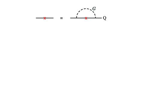
Figure 1: “Bootstrap” gap equation for generating heavy quark mass from Goldstone boson loop.

With the existence of three quark generations already, interest 4S4G has been growing in the fourth generation in the past few years, as the LHC opens up new horizons. Of course, an SM Higgs interpretation of the 126 GeV boson deflates one’s faith in the 4th generation. However, with our assumption of a heavy Higgs boson while taking the 126 GeV boson as the dilaton, the 4th generation remains a viable possibility. The pursuit has indeed been vigorous at the LHC in the past few years, where the current bound bpCMS12 ; leptCMS12 on $m_{Q}$ has reached beyond 600 GeV (we shall assume “heavy isospin” symmetry, $I_{Q}$, and treat the doublet $Q$ as degenerate). This is already above the nominal perturbative partial wave unitarity bound (UB) of 550 GeV Chanowitz78 . The Yukawa coupling $\lambda_{Q}\equiv\sqrt{2}m_{Q}/v$ is more than 3.5 times larger than $\lambda_{t}\simeq 1$, and has entered the strong coupling regime ($\alpha_{Q}\equiv\lambda_{Q}^{2}/4\pi\sim 1$).

With the ever increasing bound on $m_{Q}$, it may well not exist. But being beyond UB, it begs the question: Could the strong Yukawa coupling of $Q$ generate Holdom06 EWSB itself? Along this line, a gap equation, given symbolically in Fig. 1, was constructed Hou12 without ever invoking the Higgs doublet, or the Higgs boson field. The logic, or philosophy goes as follows. The Goldstone boson $G$ is viewed as a tightly bound (by Yukawa coupling itself!) $Q\bar{Q}$ state. It was in fact postulated Hou12 as the collapsed state by Yukawa binding, as seen through a Bethe–Salpeter equation study Jain (for further elucidation, see Ref. EHY11 ), which is taken as suggestive of triggering EWSB itself. With no New Physics in sight at the LHC, not even the heavy chiral quark $Q$ itself, the loop momentum integration runs up to roughly $2m_{Q}$, without the need to add any further effects (with the simplification of ignoring, or truncating, corrections to $G$ propagation and $GQQ$ vertex). This is therefore a “bootstrap” gap equation, in that the strong Yukawa coupling itself is the source of EWSB, or mass generation for quark $Q$, which simultaneously justifies keeping the Goldstone $G$ in the loop. The existence of a large Yukawa coupling $\lambda_{Q}$ is used as input, without a theory for $\lambda_{Q}$ itself.

The question now is whether one could find a solution to such a gap equation. If so, we would have demonstrated the case for DSB, and the potential riches that could follow. The purpose of this paper is to formulate more clearly the gap equation, and demonstrate that numerical solution does exist at strong coupling. A similar gap equation was formulated by Hung and Xiong HX11 , where $G$ in Fig. 1 is replaced by a massless Higgs doublet field. We will compare and offer a critique.

The paper is organized as follows. In the next section, after briefly mentioning the Nambu–Jona-Lasinio model, which is a simplified template for DSB where the self-energy is momentum-independent, we focus on the more relevant strongly-coupled scale-invariant QED, which we utilize as a means of setting up our approach. In Sec. III, we formulate our bootstrap gap equation following the setup in Sec. II, and solve numerically for the critical $\lambda_{Q}$ (hence $m_{Q}$). We compare with a similar study by Hung and Xiong, and pursue the consequence of taking the physical loop cutoff to be less than $2m_{Q}$, and outline the framework for further study. In Sec. IV we discuss the many questions and issues of DSB related to our bootstrap equation, including the issue of the dilaton. Our conclusion is given in Sec. V.

II Historical Backdrop for DSB

In this section we briefly review the Nambu–Jona-Lasinio model, where one sets up a gap equation with its well-known solution. We then turn to the so-called strongly-coupled scale-invariant QED, which is closer to our gap equation. By recounting some major steps, we also set up our notation for later usage.

II.1 NJL Model

The Nambu–Jona-Lasinio model NJL , proposed in 1960, is the earliest, explicit model of DSB, where the breaking of global chiral symmetry leads to generation of nucleon mass, and the pion as a (pseudo-)Goldstone boson NG .

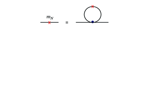
Figure 2: Gap equation for the Nambu–Jona-Lasinio model for generating nucleon mass.

The model can be depicted as in Fig. 2, where a four-fermion interaction is introduced, represented by the blob on the right-hand side. The nucleon mass, represented by a cross, is self-consistently generated. One easily finds the gap equation

$$m_{N} = \frac{N_{C}}{8\pi^{2}}G\int_{0}^{\Lambda^{2}}dq^{2}\,q^{2}\frac{m_{N}}{q^{2}+m_{N}^{2}}$$ (1)

$$= \frac{N_{C}}{8\pi^{2}}G\Lambda^{2}\left(1-\frac{m_{N}^{2}}{\Lambda^{2}}\log\left(1+\frac{\Lambda^{2}}{m_{N}^{2}}\right)\right)m_{N},$$

where $G$ here is the four-fermi coupling and $\Lambda$ is the cutoff. Since $m_{N}$ on both sides factor out, one has

$$1-\frac{G_{\rm crit}}{G} = \frac{m_{N}^{2}}{\Lambda^{2}}\log\left(1+\frac{\Lambda^{2}}{m_{N}^{2}}\right),$$ (2)

which admits a solution for $G>G_{\rm crit}$, where

$${G_{\rm crit}} = \frac{8\pi^{2}}{N_{C}\Lambda^{2}}.$$ (3)

To understand what is happening, one can iterate the cross of the left-hand side of Fig. 2 on the right-hand side, and sees that it contain an infinite number of diagrams. This effectively puts the original self-energy diagram into the denominator, and in the end, one trades the parameters $G$ and $\Lambda$ for the physical $m_{N}$ and the pion-nucleon coupling. At the more refined level and using the quark language, one can show further that the emergent Goldstone boson, the pion, is in fact a ladder sum of the quark-level four-fermi interaction.

We will return at the end to discuss the similarity and differences of the NJL model with our gap equation.

II.2 Strongly-coupled Scale-invariant QED

We note that the self-energy bubble of Fig. 2 does not depend on external momentum $p$, so at the superficial level, Fig. 2 is quite different from Fig. 1. We now turn to QED, where there is closer similarity.

The general gap equation for QED FK76 can be written in the form of the Schwinger–Dyson (SD) equation,

$$\Sigma(p)=ie^{2}\int\frac{d^{4}q}{(2\pi)^{4}}\gamma^{\mu}D_{\mu\nu}(q)S(p-q)\Gamma^{\nu}(p,q),$$ (4)

where $\Sigma=/\!\!\!p-m-S(p)^{-1}$ is the electron self-energy with $S$ the electron (full) propagator, $D_{\mu\nu}$ is the photon (full) propagator, and $\Gamma$ is the full vertex.

II.2.1 Ladder Approximation and Integral Form

Truncating the exact, full vertex and photon propagator by the approximation,

$$\Gamma^{\nu}(p,q) = \gamma^{\nu},$$ (5)

$$D_{\mu\nu}(q) = \frac{-g_{\mu\nu}+q^{\mu}q^{\nu}/q^{2}}{q^{2}}-\xi\frac{q_{\mu}q_{\nu}}{q^{4}},$$ (6)

which is called the ladder (or rainbow) approximation, the gap equation becomes

$$S(p)^{-1}=/\!\!\!p-ie^{2}\int\frac{d^{4}q}{(2\pi)^{4}}\gamma^{\mu}D_{\mu\nu}(p-q)S(q)\gamma^{\nu},$$ (7)

with $D_{\mu\nu}$ given in Eq. (6), and we have set $m=0$, i.e. massless QED (at Lagrangian level). Pictorially, this is represented as in Fig. 3. The question now is whether the scale invariance could be dynamically broken at some strong coupling $\alpha=e^{2}/4\pi$?

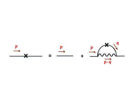
Figure 3: Gap equation for QED in the ladder approximation.

We define the electron propagator as FK76

$$S(p)=\frac{1}{A(p^{2})\,/\!\!\!p-B(p^{2})},$$ (8)

where the $A$ term corresponds to wave function renormalization, i.e. related to the usual $Z^{-1}$ factor. A finite pole of the propagator, $p^{2}=B^{2}(p^{2})/A^{2}(p^{2})$, would give the dynamical effective mass. Our aim is therefore solving $A$ and $B$ from the gap equation of Eq. (7). Inserting Eq. (6) and after some algebra, one finds

$$B(p^{2})=e^{2}\int\frac{id^{4}q}{(2\pi)^{4}}\left(\frac{-4+1-\xi}{k^{2}}\right)\frac{B(q^{2})}{A^{2}(q^{2})q^{2}-B^{2}(q^{2})},$$ (9)

and

$$A(p^{2})=1-\frac{e^{2}}{4p^{2}}{\rm tr}\int\frac{id^{4}q}{(2\pi)^{4}}\gamma^{\mu}D_{\mu\nu}^{(\xi)}\frac{A(q^{2})/\!\!\!q}{A^{2}(q^{2})q^{2}-B^{2}(q^{2})}\gamma^{\nu}/\!\!\!p.$$ (10)

II.2.2 Landau Gauge and Differential Form

Simplification can be achieved in Landau gauge, $\xi=0$, where one finds $A(p^{2})=1$. Since $A$ is the inverse of wave function renormalization, this means that it satisfies Ward-Takahashi identity even under the ladder approximation. The gap equation we need to solve is simplified to just an equation for $B$,

$$B(p^{2})=-3e^{2}\int\frac{id^{4}q}{(2\pi)^{4}}\frac{B(q^{2})}{(p-q)^{2}(q^{2}-B^{2}(q^{2}))}.$$ (11)

After Wick rotation, and using

$$\int d^{4}q\frac{f(q^{2})}{(p-q)^{2}}=\pi^{2}\int dq^{2}q^{2}\left[\frac{\theta(p-q)}{p^{2}}+\frac{\theta(q-p)}{q^{2}}\right]f(q^{2}),$$ (12)

one obtains

$$B(x)=\frac{3\alpha}{4\pi}\left(\frac{1}{x}\int_{\Lambda_{\rm IR}^{2}}^{x}dy\frac{yB(y)}{y+B^{2}(y)}+\int_{x}^{\Lambda^{2}}dy\frac{B(y)}{y+B^{2}(y)}\right),$$ (13)

where $x=p_{E}^{2}$ is the Euclidean momentum squared, and $\Lambda^{2}$, $\Lambda_{\rm IR}^{2}$ are its ultraviolet (UV) and infrared (IR) cutoffs, respectively.

The integral equation can be changed to a differential equation by noting

$$\frac{dB(x)}{dx} = \frac{3\alpha}{4\pi}\left(-\frac{1}{x^{2}}\right)\int_{\Lambda_{\rm IR}^{2}}^{x}dy\frac{yB(y)}{y+B^{2}(y)},$$ (14)

$$\frac{d(xB(x))}{dx} = \frac{3\alpha}{4\pi}\int_{x}^{\Lambda^{2}}dy\frac{B(y)}{y+B^{2}(y)}.$$ (15)

One obtains the differential equation,

$$x\frac{d^{2}B(x)}{dx^{2}}+2\frac{dB(x)}{dx}+\frac{3\alpha}{4\pi}\frac{B(x)}{x+B^{2}(x)}=0.$$ (16)

together with the boundary conditions (B.C.) for IR and UV, which are given as

$$\left.\frac{dB(x)}{dx}\right|_{x=\Lambda_{\rm IR}^{2}} = 0,\ \ \ \ \left.\frac{d(xB(x))}{dx}\right|_{x=\Lambda^{2}}=0.$$ (17)

If IR cutoff is 0, the B.C. for IR should be replaced by $2BdB/dx=-3\alpha/4\pi$ at $x=0$.

II.2.3 Analytic Solution in Landau Gauge

In order to study qualitative features, let us find first an approximate solution. In particular, for the special range for the IR cutoff, let us take $B(x)\ll\Lambda_{\rm IR}<x^{\frac{1}{2}}<\Lambda$, then Eq. (16) is simplified to

$$x^{2}\frac{d^{2}B(x)}{dx^{2}}+2x\frac{dB(x)}{dx}+\frac{3\alpha}{4\pi}{B(x)}=0.$$ (18)

The characteristic equation for solution $B(x)=Cx^{\lambda}$ is

$$\lambda(\lambda-1)+2\lambda+\frac{3\alpha}{4\pi}=0,$$ (19)

with discriminant $1-3\alpha/\pi$, hence the behavior is different for $\alpha>\alpha_{c}$ and $\alpha<\alpha_{c}$, where $\alpha_{c}=\pi/3$. The analytical solution under the approximation is given as

$$B = b_{1}\,x^{(-1+\sqrt{1-\alpha/\alpha_{c}})/2}+b_{2}\,x^{(-1-\sqrt{1-\alpha/\alpha_{c}})/2}$$ (20)

$$\equiv b_{1}\,x^{c_{1}}+b_{2}\,x^{c_{2}},$$

and the boundary conditions can be written as

$$\left(\begin{array}[]{cc}c_{2}&c_{1}\Lambda_{\rm IR}^{2(c_{1}-c_{2})}\\ -1&\Lambda^{2(c_{1}-c_{2})}\end{array}\right)\left(\begin{array}[]{c}b_{1}\\ b_{2}\end{array}\right)=\left(\begin{array}[]{c}0\\ 0\end{array}\right).$$ (27)

The determinant must vanish for nontrivial $b_{1},b_{2}$, hence

$$\frac{\sqrt{1-\alpha/\alpha_{c}}-1}{\sqrt{1-\alpha/\alpha_{c}}+1}=\left(\frac{\Lambda^{2}}{\Lambda_{\rm IR}^{2}}\right)^{\sqrt{1-\alpha/\alpha_{c}}}.$$ (28)

To satisfy this condition, $\alpha>\alpha_{c}=\pi/3$ is needed, and for given $\Lambda/\Lambda_{\rm IR}$, $\alpha$ takes on discontinuous values,

$$n\pi+\tan^{-1}\frac{1}{\sqrt{\alpha/\alpha_{c}-1}}=\sqrt{\alpha/\alpha_{c}-1}\log\frac{\Lambda}{\Lambda_{\rm IR}}.$$ (29)

One sees that $\alpha\to\alpha_{c}$ for $\Lambda/\Lambda_{\rm IR}\to\infty$, the nominal “continuum limit”. For $\alpha<\alpha_{c}$, the only solution that satisfies the B.C. is the trivial $B(x)=0$.

The approximate solution for small IR cutoff can now be obtained by replacing $B(x)=m$ (constant) for small $x$. The differential equation becomes

$$x\frac{d^{2}B(x)}{dx^{2}}+2\frac{dB(x)}{dx}+\frac{3\alpha}{4\pi}\frac{B(x)}{x+m^{2}}=0,$$ (30)

where $B(x)$ is a hypergeometric function. Namely,

$$B(x)=m\,F\left(\frac{1}{2}-i\gamma,\;\frac{1}{2}+i\gamma,\;2;\ -\frac{x}{m^{2}}\right),$$ (31)

where

$$i\gamma=\frac{1}{2}\sqrt{1-\frac{\alpha}{\alpha_{c}}},\qquad\alpha_{c}=\frac{\pi}{3},$$ (32)

and $F$ is a hypergeometric function. Checking the asymptotic behavior for $x\gg m^{2}$, the power behavior for $\alpha<\alpha_{c}$ cannot satisfy the UV boundary condition.

The gap equation has a nontrivial or oscillatory solution for $\alpha>\alpha_{c}$, where the critical coupling is $\alpha_{c}=\pi/3$ for QED. The dynamical effective mass is obtained by solving $x=B^{2}(-x)$. Note that the pole of the propagator should be given in the time-like region, so one has to make analytical continuation in order to obtain a physical mass, which can be done smoothly for $\Lambda_{\rm IR}\to 0$.

An issue arises in that the dynamical mass

$$m=4\Lambda\,e^{-\frac{\pi}{\sqrt{\alpha/\alpha_{c}-1}}}.$$ (33)

is proportional to the UV cutoff $\Lambda$. For $m$ to be physical, however, it should not depend on $\Lambda$. Miransky suggested Miransky that $\alpha\to\alpha_{c}$ as $\Lambda\to\infty$, i.e. $\alpha_{c}$ is a nontrivial UV fixed point. A related issue, which we would not go into, is whether there would be a dilaton associated with breaking of scale invariance dilaton1 .

III Bootstrap Dynamical EWSB

For the gap equation Hou12 with large empirical Yukawa coupling, one could continue to follow the Fukuda–Kugo approach of the previous section. In Landau gauge ($\xi=0$), the propagation of (would-be) Goldstone modes and gauge bosons are properly separated, and the gap equation becomes equivalent to our discussion below if one takes the $g\to 0$ limit for the gauge coupling. The Goldstone $G^{\pm}$ and $G^{0}$ couple to fermions with the familiar Yukawa couplings, which we have argued Hou12 as experimentally established. They are also unaltered by the $g\to 0$ limit. The main assumption is the addition of a new (heavy) chiral quark doublet, where the $I_{Q}$ heavy isospin implies that $\lambda_{U}=\lambda_{D}\equiv\lambda_{Q}$, i.e. equality of the $I_{Q3}=\pm\frac{1}{2}$ Yukawa couplings. We ask whether large $\lambda_{Q}$ could be the source of EWSB, through the conceptual gap equation of Fig. 1.

III.1 Ladder Approximation

In any case, we do not know the full propagator and vertex functions. We approximate the Goldstone-fermion vertex as undressed, and the Goldstone propagator remains as $i/k^{2}$, analogous to the QED treatment in previous section. Similar to Fig. 3, the gap equation for large Yukawa (vanishing $g$) coupling is depicted in Fig. 4. It is interesting to note that, while $m_{0}=0$ for strong QED was set by hand, in the present case, $m_{0}=0$ is by gauge (or chiral, in $g\to 0$ limit) invariance.

We aim at solving for quark propagator $S(p)$, given as

$$S(p)^{-1}=A(p^{2})\,/\!\!\!p-B(p^{2}),$$ (34)

which is in same form as Eq. (8) for QED. Following similar steps as in Sec. II, and assuming $\lambda_{U}=\lambda_{D}=\lambda_{Q}$ degeneracy, we obtain

$$B_{p^{2}} =\frac{3\lambda_{Q}^{2}}{2} \int\frac{d^{4}q}{i(2\pi)^{4}}\frac{1}{(p-q)^{2}}\frac{B_{q^{2}}}{q^{2}A^{2}_{q^{2}}-B^{2}_{q^{2}}}$$ (35)

$$-\frac{\lambda_{Q}^{2}}{2} \int\frac{d^{4}q}{i(2\pi)^{4}}\frac{1}{(p-q)^{2}-m_{h}^{2}}\frac{B_{q^{2}}}{q^{2}A^{2}_{q^{2}}-B^{2}_{q^{2}}},$$

and

$$A_{p^{2}}=1+ \frac{3\lambda_{Q}^{2}}{2p^{2}} \int\frac{d^{4}q}{i(2\pi)^{4}}\frac{p\cdot q}{(p-q)^{2}}\frac{A_{q^{2}}}{q^{2}A^{2}_{q^{2}}-B^{2}_{q^{2}}}$$

$$+ \frac{\lambda_{Q}^{2}}{2p^{2}} \int\frac{d^{4}q}{i(2\pi)^{4}}\frac{p\cdot q}{(p-q)^{2}-m_{h}^{2}}\frac{A_{q^{2}}}{q^{2}A^{2}_{q^{2}}-B^{2}_{q^{2}}},$$ (36)

where placement of $i$ anticipates the Wick rotation, and $B_{q^{2}}$ stands as shorthand for $B(q^{2})$, and likewise for $A$. We have already used $\xi=0$, so, compared to massless QED, we now have to consider $A$, or wave function renormalization effects, hence a coupled set of equations for $A(p^{2})$ and $B(p^{2})$. Note that we have kept a “Higgs” term, applying Standard Model Higgs boson, $h^{0}$, couplings. This is for purpose of later comparison with the work of Hung and Xiong HX11 .

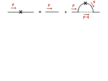
Figure 4: Gap equation for large Yukawa coupling in the ladder approximation, where $m_{0}$ vanishes by gauge (or chiral) invariance.

If one simply drops the second term (no physical Higgs, or taking $m_{h}\sim\infty$), so only Goldstone modes propagate, the gap equation becomes, after angular integration and Wick rotation,

$$B(x) = \kappa_{b}\left(\frac{1}{x}\int_{\Lambda_{\rm IR}^{2}}^{x}dy\frac{yB(y)}{yA^{2}(y)+B^{2}(y)}\right.$$ (37)

$$\left.\quad\;\ \ +\int_{x}^{\Lambda^{2}}dy\frac{B(y)}{yA^{2}(y)+B^{2}(y)}\right),$$

$$A(x)=1 + \kappa_{a}\left(\frac{1}{x^{2}}\int_{\Lambda_{\rm IR}^{2}}^{x}dy\frac{y^{2}A(y)}{yA^{2}(y)+B^{2}(y)}\right.$$ (38)

$$\left.\quad\quad\;+\int_{x}^{\Lambda^{2}}dy\frac{A(y)}{yA^{2}(y)+B^{2}(y)}\right),$$

where

$$\kappa_{b}=2\kappa_{a}=\frac{\frac{3}{2}\lambda_{Q}^{2}}{16\pi^{2}}=\frac{\frac{3}{2}\alpha_{Q}}{4\pi}.\quad\quad{\rm(no\ Higgs)}$$ (39)

Had we taken the limit $m_{h}\to 0$ in Eqs. (35) and (36) to mimic the Hung-Xiong approach of a massless scalar doublet, then

$$\kappa_{b}=\kappa_{a}=\frac{\lambda_{Q}^{2}}{16\pi^{2}}=\frac{\alpha_{Q}}{4\pi}.\quad\ {\rm(massless\ Higgs)}$$ (40)

We keep the notation of $\kappa_{b}$ and $\kappa_{a}$ in Eqs. (39) and (40) to cover these two cases.

Analogous to Sec. II, Eqs. (37) and (38) can be put into differential form,

$$xB^{\prime\prime}+2B^{\prime}+\frac{\kappa_{b}B}{xA^{2}+B^{2}}=0,$$ (41)

$$xA^{\prime\prime}+3A^{\prime}+\frac{2\kappa_{a}A}{xA^{2}+B^{2}}=0,$$ (42)

with the boundary conditions

$$\left.B^{\prime}(x)\right|_{x=\Lambda^{2}_{\rm IR}} = 0,\ \left(xB^{\prime}(x)+B(x)\right)|_{x=\Lambda^{2}}=0,$$ (43)

$$\left.A^{\prime}(x)\right|_{x=\Lambda^{2}_{\rm IR}} = 0,\ \left(\frac{1}{2}xA^{\prime}(x)+A(x)\right)|_{x=\Lambda^{2}}=1,$$ (44)

where prime stands for $x$-derivative.

We note at this point that, if one ignores wave function renormalization, i.e. Eq. (42), while forcefully setting $A(x)=1$ in Eq. (41), then one has the same solution as in QED, with the change in critical coupling

$$\alpha_{Q}^{c}=\frac{2\pi}{3},$$ (45)

which is twice as high as for QED, and

$$\lambda^{c}_{Q}=2\pi\sqrt{\frac{2}{3}}\simeq 5.13,$$ (46)

hence superficially a “critical mass” $m_{Q}^{c}\simeq 890$ GeV, which is above current LHC limits bpCMS12 ; leptCMS12 . But it should be clear that the wave function renormalization $A(p^{2})$ term cannot be neglected foot .

III.2 Numerical Solution

Redefining $p^{2}=x=e^{2t}$, our target simultaneous differential equations with B.C. become

$$\ddot{B}+2\dot{B}+\frac{4\kappa_{b}B}{A^{2}+B^{2}e^{-2t}}=0,$$ (47)

$$\ddot{A}+4\dot{A}+\frac{8\kappa_{a}A}{A^{2}+B^{2}e^{-2t}}=0,$$ (48)

$$\dot{B}(t_{\rm IR})=0,\;\ \quad\dot{B}(t_{\rm UV})+B(t_{\rm UV})=0,$$ (49)

$$\dot{A}(t_{\rm IR})=0,\quad\frac{1}{4}\dot{A}(t_{\rm UV})+A(t_{\rm UV})=1,$$ (50)

where dot represents $t$-derivative, and $e^{t_{\rm UV}}=\Lambda_{\rm UV}=\Lambda$, and $e^{t_{\rm IR}}=\Lambda_{\rm IR}$.

III.2.1 Asymptotic Properties

Due to scale invariance, the differential equations are invariant under

$$x\to a^{2}x\qquad(t\to t+\log a),$$ (51)

$$\Lambda_{\rm UV,IR}\to a\Lambda_{\rm UV,IR},$$ (52)

$$B\to aB,\quad A\to A.$$ (53)

As a result, the solutions of the differential equations depend only on $\Lambda_{\rm UV}/\Lambda_{\rm IR}$ ($=e^{t_{\rm UV}-t_{\rm IR}}$) and $m_{\rm dyn}\equiv B(t_{\rm IR})/A(t_{\rm IR})$ for given $\kappa_{a}$ and $\kappa_{b}$. Thus, $m_{\rm dyn}$ is a kind of integration constant. We will see that the most important feature of the solutions is that only special values (discontinuous values) of $\kappa_{a}$ and $\kappa_{b}$ are allowed for given boundary conditions.

If we take $\kappa_{a}=0$, the equations can be solved analytically, and the solution can be described as in the case of strong coupling QED with Landau gauge, Eqs. (20)–(28). The property illustrated for $\kappa_{a}=0$ should hold also for $\kappa_{a}\neq 0$, where, depending on $\Lambda_{\rm UV}/\Lambda_{\rm IR}$, $\kappa_{a}$ should take on special discontinuous values to satisfy the gap equation for the cases of $\kappa_{a}/\kappa_{b}=1$ or $1/2$.

To see this, we note that the $B^{2}e^{-2t}$ term in the denominators are irrelevant. This is because for $t\ll\log m$, the $t$ dependence of $A$ and $B$ are negligible due to the boundary conditions $\dot{A}(t_{\rm IR})=\dot{B}(t_{\rm IR})=0$. Therefore, to understand the behavior of the solution, one can take $t_{\rm IR}\sim\log m$ and consider the differential equation with $B^{2}e^{-2t}$ dropped:

$$\ddot{B}+2\dot{B}+\frac{4\kappa_{b}B}{A^{2}}=0,$$ (54)

$$\ddot{A}+4\dot{A}+\frac{8\kappa_{a}}{A}=0,$$ (55)

where the equation for $A$ becomes independent from $B$, but its solution affects $B$.

The solution of $A$ is obtained analytically:

$$A(x) = A_{0}\frac{\Lambda_{\rm UV}^{4}}{x^{2}}e^{-\zeta^{2}}\sqrt{\frac{\kappa_{a}}{\pi}},$$ (56)

$$\zeta = {\rm Erf}^{-1}\left[\frac{1}{A_{0}}\left(1-\frac{x^{2}}{\Lambda_{\rm UV}^{4}}\right)+{\rm Erf}\left(\frac{1}{\sqrt{\kappa_{a}}}\right)\right],$$ (57)

where $A_{0}$ is an integration constant which can be fixed by the B.C. for IR. Using the analytical solution, one can show that only discontinuous values of $\kappa_{a,b}$ can satisfy the B.Cs. The “critical” value of $\kappa_{b}$ can be easily obtained numerically, even without neglecting $B^{2}e^{-2t}$ term in the denominators. Of course, since the solutions are found numerically, it is not a proof that one really has a “critical” value. The upshot is that only special values of the coupling can satisfy the SD equation for given values of $\Lambda_{\rm UV}/\Lambda_{\rm IR}$ for $m_{\rm dyn}<\Lambda_{\rm IR}$ (or $\Lambda_{\rm UV}/m_{\rm dyn}$ for $m_{\rm dyn}>\Lambda_{\rm IR}$), where $m_{\rm dyn}=B(\Lambda_{\rm IR})/A(\Lambda_{\rm IR})$.

Our numerical solution gives

$$\kappa_{b}^{c}\simeq 1.4\;\,\qquad(\kappa_{b}=2\kappa_{a}=3\alpha_{Q}/8\pi),$$ (58)

$$\kappa_{b}^{c}\simeq 13.7\qquad(\kappa_{b}=\kappa_{a}=\alpha_{Q}/4\pi).$$ (59)

corresponding to

$$\lambda_{Q}^{c}\simeq 12\qquad(\kappa_{b}=2\kappa_{a}=3\alpha_{Q}/8\pi),$$ (60)

$$\lambda_{Q}^{c}\simeq 46\qquad(\kappa_{b}=\kappa_{a}=\alpha_{Q}/4\pi),$$ (61)

where the latter case is much higher. Here $c$ stands for “critical”, and our numerical values are extracted in the large $\Lambda_{\rm UV}/\Lambda_{\rm IR}$ and $\Lambda_{\rm UV}/m_{\rm dyn}$ limit. Note that for the case of $\kappa_{a}=0$ (i.e. $A=1$), the critical value was $\lambda_{Q}^{c}\simeq 5.1$, Eq. (46).

The values in Eqs. (60) and (61) corresponds to effectively taking $\Lambda_{\rm UV}\to\infty$, which is certainly not the range of validity for Eq. (60) as a descendent of Fig. 1. That is, the conceptual foundation for Fig. 1 is that, for momentum roughly up to somewhere below $2m_{Q}$, corrections to the Goldstone boson propagator and vertex has been ignored. Nevertheless, at face value, if we naively apply the physical $v\simeq 246$ GeV, then Eqs. (60) and (61) imply the mass values

$$m_{Q}^{c}>2.1\ {\rm TeV},\quad\quad{\rm(No\ Higgs)}$$ (62)

and 8.1 TeV, respectively, which are rather high. We no longer display the latter, “massless Higgs” (or light Higgs) case, not only because it is clearly out of reach for the LHC, but for theoretical reasons as we explain below. The lower bound nature of Eq. (62) would be explained subsequently.

III.2.2 Comparison with work of Hung and Xiong

We now make some comparison with, and offer a critique of, the approach of Hung and Xiong HX11 (HX). We have mimicked the concept of HX by keeping a “Higgs” scalar contribution in Eqs. (35) and (36), which resulted in the second case of Eq. (40) in the limit of $m_{h}\to 0$, as compared with our case of interest, Eq. (39), where we drop the $m_{h}$-dependent term.

HX assumed the existence of a massless Higgs doublet, where our Eqs. (41) and (42) with Eq. (40) should be a faithful representation. However, not only is the massless doublet assumed, HX ignored wave function renormalization, i.e. the $A$ term, in the treatment of their gap equation. Furthermore, the sign of our second integral in Eq. (35) disagrees with HX, suppressing the coefficient of $\lambda_{Q}^{2}$ in comparison. In the earlier work Hou12 that set up the gap equation of Fig. 1, taking the numerics of HX, the estimate of $\lambda_{Q}^{c}=\sqrt{2}\pi$ (compare Eq. (46)) gave $m_{Q}^{c}\simeq 770$ GeV, which is not too far above the current LHC bound. But with our sign for the second integral in Eq. (35), we would arrive at $\lambda_{Q}^{c}=2\pi$, or $m_{Q}^{c}\sim 1.1$ TeV, i.e. a factor of $\sqrt{2}$ higher. With our results, the Higgs boson effect would cancel out part of the Goldstone effect, hence requiring stronger Yukawa coupling.

But we have argued that it is not justified to ignore the wave function renormalization effect of $A(p^{2})$. After all, the boson loop has momentum dependence, so it would necessarily affect the $Z$ factor. Thus, the above simple numerics is incorrect. Keeping $A$ in our numerical study, hence the coupled $A$–$B$ equations, a considerably higher critical $m_{Q}^{c}$ is found. For the case of taking $\kappa_{b}=\kappa_{a}=\lambda_{Q}^{2}/16\pi^{2}$, Eq. (40), where we mimic HX’s massless Higgs doublet effect, the critical $\lambda_{Q}^{c}$ of Eq. (61) is almost 4 times as high as that for Eq. (60). In fact, we obtain the $A(\Lambda_{\rm UV}^{2})=2.7$, which is quite different from 1.

Our criticism goes far deeper. Taking a scalar doublet as massless, such that superficially one has “scale-invariance”, is totally ad hoc. Effectively one has to hold the parameters of the Higgs potential such that the Higgs field always remains massless. However, there is no principle by which this scale-invariance or masslessness of the Higgs field can be maintained. After all, one is invoking large Yukawa couplings, which feed the notorious divergent quadratic corrections to the Higgs boson mass. The one-loop two-point and four-point functions with quark $Q$ in the loop would generate effective $\mu^{2}$ and $\lambda$ self-coupling terms for the Higgs field. With no explicit dynamical principle (such as gauge invariance for the case of QED), the assumption of a massless Higgs doublet as the agent of DSB is not only ad hoc, but clearly unsustainable.

In contrast, we see the merit, as well as the meaning, of our “bootstrap” gap equation. So long we are in the broken phase, there is a massless Goldstone boson, which couples with the known Yukawa coupling. Treating the Yukawa coupling as large, if a nontrivial solution to the gap equation is found (as we have illustrated above), it in turn justifies the use of a massless Goldstone boson in the gap equation. In fact, the physical argument Hou12 was to view the Goldstone boson $G$ as an extremely tight ultrarelativistic bound state of heavy $Q$ and $\bar{Q}$ from the broken phase, while $G$ enters the “bootstrap” gap equation to dynamically generate $m_{Q}$ hence break the symmetry, and in same stroke justify its own existence.

From the argument above, we see that our bootstrap gap equation puts the existence of the physical Higgs boson in doubt. After all, it is rather difficult to keep a light physical Higgs boson, in the presence of much stronger Yukawa couplings than the top quark. For our gap equation, one also cannot ignore corrections to the Higgs propagator. At the foundation level Hou12 , unlike the Goldstone boson, even though a 126 GeV Higgs-like boson has appeared, its true nature has to be settled by experiment. Our numerical study also shows that keeping the Higgs term tends to raise the critical Yukawa coupling considerably, implying $2m_{Q}$ higher than the LHC collision energy. Thus, in the name of simplicity and pertinence, we drop the $\kappa_{b}=\kappa_{a}$ case from now on. However, we shall return at the end to discuss the dilaton issue.

III.2.3 Physical Cutoff of $2m_{Q}<\Lambda_{\rm NP}$

The previous comparison with Hung-Xiong approach, and in particular the bootstrap nature of the Goldstone boson $G$ in the gap equation, illustrates that the limit $\Lambda_{\rm UV}\to\infty$ would take us outside the range of validity of the gap equation itself. It is clear that, for timelike $p^{2}>(2m_{Q})^{2}$, there is no Goldstone boson. Thus, for the cutoff $\Lambda$, one should not use the traditional language of $\Lambda_{\rm UV}$, and one probably should not contemplate “UV-completion” at the current stage. The bootstrap gap equation does not provide a theory of the heavy quark Yukawa coupling $\lambda_{Q}$, but employs it for DSB. Thus, we suggest a cutoff $\Lambda<2m_{Q}<\Lambda_{\rm NP}$, where $\Lambda_{\rm NP}$ is some true New Physics scale where the origin of Yukawa couplings may be contemplated, but it is out of reach for now.

Another possible interpretation of this cutoff is related to the restoration of symmetry. The Goldstone boson couples to broken currents, but the $Z$ factor of the Goldstone boson may vanish at some scale related to the scale where the Goldstone boson becomes unbounded, and symmetry is restored. Rather than a true $\Lambda_{\rm UV}$ that in principle extends to infinity, there exists a cutoff $\Lambda$ of the gap equation. We are in effect summing over the Goldstone boson correction to the self-energy of the quark $Q$, when the Goldstone boson is still defined. As noted in Ref. Hou12 , this picture does receive experimental support, in that no New Physics seem to be there below $\sim$ TeV scale. So, one sums up only the effect of the Goldstone boson, and nothing else.

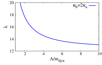
Figure 5: Cutoff dependence of Yukawa coupling, where the cutoff $\Lambda$ is in units of the dynamical quark mass $m_{\rm dyn}$.

The gap equation sums up the effect, from low to high momentum, of the correction by the Goldstone boson $G$ to the quark self-energy. Eq. (60) reflects taking this sum to $\Lambda_{\rm UV}\to\infty$. Since the summation is accumulative, if now one sums only to some $\Lambda\lesssim 2m_{Q}$, as we have argued, then the cumulative effect is less than summing to very large momentum above $2m_{Q}$. We note that $2m_{Q}$ is a physical scale parameter that is external to the scale-invariant gap equation. Nevertheless, we can plot the dependence of $\lambda_{Q}^{c}$ on the cutoff $\Lambda$. From Fig. 5, one can see that, for a lower cutoff, $\lambda_{Q}^{c}$ has to be higher than in Eq. (60). This is because, as the integration range is smaller, a larger $\lambda_{Q}$ value is needed to compensate. Thus, Eq. (60) gives a lower bound on $m_{Q}$. If we take $\Lambda=2m_{Q}$, then $\lambda_{Q}^{c}\sim 17.7$, and

$$m_{Q}\sim 3\ {\rm TeV},\quad\quad{\rm(No\ Higgs;\ }\Lambda=2m_{Q})$$ (63)

which is very high. We will return to discuss whether this could be an overestimate later.

III.2.4 Decay Constant and Yukawa Coupling

Up to now, we have been cavalier in the relation between $\lambda_{Q}^{c}$ and $m_{Q}^{(c)}$, treating it as $\sqrt{2}m_{Q}^{(c)}=\lambda_{Q}^{c}v$. But $v$ is a physically measured value, and $m_{Q}$ is yet to be experimentally measured. If electroweak symmetry is indeed dynamically broken by the large Yukawa coupling of a new heavy chiral quark $Q$, when $Q$ is discovered in the future, likely $m_{Q}>m_{Q}^{c}$. We then see that the actual v.e.v. value, $v$, may not correspond to the critical value $\lambda_{Q}^{c}$. This brings about the question of how scale invariance is actually broken in our gap equations, and whether there might be a dilaton dilaton2 . This is an extremely interesting question, given the possibility, needed for the viability of our gap equation, that the observed 126 GeV Higgs-like boson might actually be a dilaton. Our framework, however, does not provide the means to approach this problem, as it is empirical and shuns the UV.

Rather than approach this deeper problem, we try to obtain the decay constant $f_{G}$ of the Goldstone boson, which should be the same as the vacuum expectation value, $v$. Following the Pagels–Stokar formula Pagels79 naively, we obtain,

$$f_{G}^{2}=\frac{N_{C}}{4\pi^{2}}\int_{0}^{\Lambda^{2}}dx\frac{xB(x)^{2}-\frac{1}{4}x(B(x)^{2})^{\prime}}{(xA(x)^{2}+B(x)^{2})^{2}}.$$ (64)

More generally, we write

$$f_{G}^{2} = \int_{0}^{\Lambda^{2}}dx{\cal F}[A(x),B(x)]$$ (65)

$$= m_{Q}^{2}\int_{0}^{\Lambda^{2}/m_{Q}^{2}}d\hat{x}\hat{\cal F}[A(\hat{x}),B(\hat{x})/A(\hat{x})/m_{Q}],$$

where $m_{Q}\equiv B(0)/A(0)$, and we have scaled by $m_{Q}$ (and redefined the function ${\cal F}$), treating it as physical.

We can get back the “Yukawa” coupling $\lambda$ (it should really be denoted as $Y$, and the question is whether $Y=\lambda$) for the input to the gap equation, or

$$\frac{1}{2\lambda^{2}}=\int_{0}^{\Lambda^{2}/m_{Q}^{2}}d\hat{x}\hat{\cal F}[A(\hat{x}),B(\hat{x})/A(\hat{x})/m_{Q}].$$ (66)

If the system is really scale-invariant, the r.h.s. of Eq. (66) is a function of $\Lambda/m_{Q}$ and $\lambda$. In order to satisfy the gap equation, $\lambda$ is obtained as a function of $\Lambda/m_{Q}$. Namely, it should not depend on $m_{Q}$ explicitly. Taking the cutoff $\Lambda=2m_{Q}$, the equation becomes iterative for $\lambda$. Therefore, solving the gap equation, we obtain a prediction for the heavy quark mass. But technical issues remain: Is $m_{Q}$ a physical mass? What about the infrared cutoff? Can our assumption of $\lambda(\Lambda_{\rm UV}/m_{Q})=Y(\Lambda_{\rm UV}/m_{Q})$ be maintained self-consistently? We leave these theoretical questions to a future work.

IV Discussion

$\bullet$ Can $m_{Q}$ be brought lower than 2–3 TeV?

From a phenomenlogical standpoint, our numerical value of $m_{Q}\sim 3$ TeV of Eq. (63), even the 2 TeV value of Eq. (62), seem depressingly high. We offer a few remarks how this might be lowered. In the spirit of Refs. Hou12 and EHY11 , the Goldstone boson $G$ is the lowest or most tightly bound state through the Yukawa coupling itself. Yukawa-bound resonances exist above this isotriplet, color-singlet, pseudoscalar state, the leading ones being the isotriplet, pseudoscalar $\pi_{8}$, the isosinglet, vector $\omega_{8}$, which are both color-octet, and the isosinglet, vector, color-singlet $\omega_{1}$ “mesons”. Without solving the strongly coupled bound state problem, one does not know the spectrum (i.e. how tightly they are bound below $2m_{Q}$), nor their “decay constants”, i.e. how they couple to the heavy quark $Q$. But the couplings should be rather strong. The point is, as one integrates the Goldstone loop up to $2m_{Q}$, at some point these heavy mesons should also enter, and contribute in the same spirit to the self-energy of $Q$.

There is thus some hope that extra, attractive contributions could lower $\lambda_{Q}^{c}$. But it also illustrates the limits of our bootstrap approach. The momentum integration for these extra contributions start from the meson mass, up to $2m_{Q}$, but clearly the meson propagators and the meson-$QQ$ vertices would be much more sensitive to $q$ as it varies, compared to the Goldstone boson $G$. Even for $G$ (which is the $\pi_{1}$), as one approaches $2m_{Q}$, its bound state nature would lead to modifications of its propagator (even if symmetry remains broken hence it remains massless) and vertex.

$\bullet$ Self-consistency with Dilaton

We have already offered our critique of the work of Hung and Xiong HX11 , and showed also numerically that the needed $\lambda_{Q}^{c}$ is exorbitantly high if one includes a light SM Higgs. Thus, if the new 126 GeV boson is found to be truly the SM Higgs, our bootstrap DSB gap equation cannot work. However, we have argued that the nature of the new boson probably cannot be demonstrated beyond doubt with 2011-2012 LHC data, and a loophole is the dilaton dilaton ; dilaton2 . The dilaton is allowed by our gap equation, since the DSB also breaks scale invariance.

At the operational level, one can easily see that, if the observed 126 GeV object is a dilaton, it does not change the main result of our study. That is, given that the dilaton coupling is suppressed by $v/f$ compared to the SM Higgs boson, where $f$ is the dilaton decay constant, the $m_{h}$-dependent terms of Eqs. (35) and (36) are suppressed by $v^{2}/f^{2}$, and can be treated as subdominant hence dropped, in the same spirit that the strong and weak gauge couplings are treated as subdominant.

$\bullet$ Comparison with NJL-type Models

A different question is whether our gap equation is actually equivalent to the NJL model. We have already commented that for the NJL model, the self-energy does not depend on momentum, and one simply cuts the loop momentum off at some $\Lambda$. For our gap equation, the wave function part, $A$, has momentum dependence, i.e. the Yukawa loop always modifies the $Z$ factor. We already saw this in scale-invariant QED. For NJL, the cutoff $\Lambda$ is traded, together with the associated dimension $-2$ coupling constant $G$, for the physical $f_{\pi}$ and $m_{N}$, although, depending on the cutoff, there is a critical coupling $G_{\rm crit}$ (see Eq. (3)). For our case, one cannot take arbitrary values for the cutoff. Instead, we argued that, because the Goldstone boson would become unbounded at some scale, say $2m_{Q}$, the cutoff of the loop momentum has to be “heuristically” finite. Further similarities and differences are noted in Ref. Hou12 . A fundamental difference may be that one has effectively postulated that the dimension zero Yukawa coupling of the Goldstone boson to be the experimentally verified one related to the left-handed vector gauge coupling of massive quarks. If the Goldstone boson $G$ is an ultratight $Q\bar{Q}$ bound state, it has turned the effective $Q\bar{Q}$ dimensionality to 1. In this sense, our gap equation may resemble the gauged NJL model dilaton1 , in which the dimensionality of the bound state tends to 1 near the critical gauge coupling.

Our approach is also conceptually different from those descended from the top condensation model top_condense , in which the gauged NJL is applied to EWSB. The self-energy in the top condensation model incorporates both our Fig. 2 (loop with four-quark operator) and Fig. 3 (but with gauge boson in the loop). The gap equation with the four-quark operator is equivalent to the minimization of the linear sigma model with a compositeness condition, such that the Yukawa and Higgs quartic couplings blow up at the composite scale. Naively speaking, our gap equation of Fig. 4 corresponds to the linear sigma model with large Yukawa coupling. One can therefore read off the schematic correspondence between top condensation and our approach by replacing gauge coupling with Yukawa coupling, and four-quark operator loop by possible heavy bound state loop that we have discussed earlier. In the top condensation model, the four-quark interaction generates the large Yukawa coupling, and thus, it is clear that it differs from our approach. We did not touch the origins of Yukawa couplings at all.

$\bullet$ Phenomenology at LHC?

Can our high quark mass of a couple of TeV, with the associated ultra strong Yukawa coupling, be testable at the LHC? First, as we mentioned already, with this setup, it is very hard to believe that there would be a light Higgs at 126 GeV, hence the observed new boson ought to be a dilaton dilaton ; dilaton2 , which can be checked experimentally. Furthermore, one expects a heavy Higss $m_{H}>600$ GeV, and the search for heavy Higgs boson should continue to be pursued.

But even though there may be scalar resonances, experience from hadronic physics (the $\sigma$ resonance) suggest that this path may be rather murky. So, besides the current search approach that assumes QCD pair production of $Q\bar{Q}$, followed by free quark $Q$ decay, what else might one do at the LHC? After all, 2 or 3 TeV heavy quarks are approaching the searchable limits even for the high luminosity LHC running at 14 TeV. It was pointed out recently by one of us Hou12-2 , making analogy with $\bar{p}p\to n\pi$ annihilation, that the search strategy should contain $\bar{Q}Q\to nV_{L}$, where $V_{L}$ is nothing but the Goldstone bosons $G$ of the electroweak sector. It was argued that the multiplicity would be high, and behave as thermal emission from a “fireball” with temperature $T$ that is related to the v.e.v. scale $v$. If the bound states, especially $\omega_{8}$, decay in a similar way via multi-$V_{L}$, then there is good hope for such spectacular phenomena at the LHC. A corollary Hou12-2 is that the $V_{L}V_{L}\to V_{L}V_{L}$ channel may be the wrong path for going beyond heavy Higgs search, but it rather should be $V_{L}V_{L}\to nV_{L}$. What is intriguing is that the physically measured $g_{\pi NN}$ coupling is consistent with $\lambda_{\pi NN}\equiv\sqrt{2}m_{N}/f_{\pi}$, and is rather similar in value to Eq. (60). This offers a totally separate argument, hence giving confidence, that $m_{Q}$ is in fact of order 2 TeV or above.

$\bullet$ Revisiting Fermi–Yang Model

Having made the analogy of $G$-$Q$ with $\pi$-$N$, it brings back the question of whether the pion could really have been an $N\bar{N}$ bound state, i.e. whether the original conjecture of Fermi and Yang FY49 , could have been realized. The strength of $\pi NN$ coupling is simply staggering. But subsequent developments in hadron physics experiment relatively quickly gave rise to meson states in 500 to 800 MeV range (and corresponding baryon resonances), eventually exploding, in 1 to 2 GeV range, i.e. below $2m_{N}$. Thus, our gap equation does not apply. Even if one employed our gap equation, one cannot integrate the pion loop up to $2m_{N}$: the integral is cutoff at a scale $\sim\Lambda_{\rm QCD}$ that is quite below $2m_{N}$. And it turned out that $\pi$ and $N$ were QCD bound states of fermi size, so the pion was not an ultratight bound state of $N$ and $\bar{N}$.

But the possible existence of a very heavy chiral doublet offers us another chance. If the $Q\bar{Q}$ ultratight bound state picture for the Goldstone $G$ could be realized according to our bootstrap gap equation, it would strengthen our reasoning Hou12 that the underlying theory for Yukawa couplings cannot be a simple mock-up of QCD, such as (the various forms of) technicolor (TC).

We do not have new insight on bound state phenomena, other than what is already discussed in Ref. EHY11 . Unfortunately, this reference was very conservative and did not discuss above $m_{Q}>700$ GeV, as the Bethe–Salpeter (BS) equation approach tend to have collapsed states. But this was, in turn, the foundation for the postulate made in Ref. Hou12 that the leading collapsed state, $\pi_{1}$, is precisely the Goldstone boson $G$, which lead to the present gap equation study.

We do not yet know whether our gap equation could shed any light on the $Q\bar{Q}$ bound state spectra. The SD equation itself is of course a “higher level” one than the BS equation for bound state. If the BS equation Yukawa-boundstate approach can be a guide for $m_{Q}$ as high as 2 TeV, i.e. with $\alpha_{Q}>1$, the noteworthy point is that the leading bound states EHY11 $\omega_{1}$, $\omega_{8}$ and $\pi_{8}$ are rather distinct from the $\rho$s and $\eta$s of TC. Since $\rho$-like states are the typical working assumption for DSB that tends to adopt the QCD or TC mindset, we wish to stress this distinguishing aspect of Yukawa-induced DSB.

$\bullet$ Question of Flavor vs EWSB

Bound states in our approach emerge from strong Yukawa coupling (rather than QCD-like gauge dynamics as in TC), but we did not offer any theory of Yukawa couplings. This may be an advantage: By simply employing Yukawa couplings, we inherit this well tested part of the SM, including the flavor sector.

The three generation SM can account for all observed flavor and CP violation phenomena, with only minor tensions after a decade of detailed scrutiny by the B factories. Note that the Higgs boson does not enter flavor processes of interest, such as box and electroweak penguin diagrams; all interesting effects arise from Goldstone couplings. Extending to a 4th generation to address EWSB by strong Yukawa coupling, we will not encounter the usual issues of “flavor scale” as in most other approaches. Mixing of the 4th generation with lower ones must be suppressed, as the LHCb experiment finds all key measurements, such as CP phase in $B_{s}\to J/\psi\phi$, $A_{\rm FB}$ in $B\to K^{*}\mu\mu$, as well as $B_{s}\to\mu\mu$ are all consistent with SM. But this follows the well known pattern that CKM matrix elements trickle down in strength as one goes far off-diagonal. We do note that, having a 4th generation could seemingly provide enough CP violation strength HouCPV4 for matter dominance of the Universe, which can be viewed as an independent motivation for continuing to entertain the 4th generation.

Thus, unlike most approaches that suffer the dilemma of need for TeV scale physics to “stabilize the Higgs” (or EWSB) on one hand, while having a much higher flavor scale, in our case, the flavor physics scale need not be that far off. If realized, the actual origins of Yukawa couplings would become the focus question.

We mention in passing that our gap equation can be easily extended to finite temperature, allowing one to potentially explore issues related to electroweak phase transition, which is a direction that we would take up in a subsequent work.

V Conclusion

Despite the emergence of a Higgs-like new boson with mass of order 126 GeV at the LHC, we have inspected current data up to 17–18 fb^-1 level, and concluded that a dilaton interpretation cannot be fully ruled out, even if it appears fortuitous. Assuming this state as a dilaton that feigns (for now) the SM Higgs boson, while the actual Higgs boson is above 600 GeV and heavy, we consider seriously the possibility of electroweak symmetry breaking driven by strong Yukawa coupling.

Starting from a purely empirical basis, a dynamical gap equation is argued, treating the Goldstone as massless inside the loop, coupling with chiral quark doublet $Q$ with the usual Yukawa couplings. By empirical we mean the traditional sense of based on experimentally established facts, where we have utilized electroweak gauge symmetry and its spontaneously broken nature, only extending by a new chiral doublet $Q$ — the 4th generation — with Yukawa coupling $\lambda_{Q}$ already above the nominal unitarity bound, which is again empirical. The gap equation effectively sums over exchange momentum of $Q\bar{Q}$ scattering. We further utilize the experimental fact that there are no obvious new states below 1 or 2 TeV, hence this integration range can extend up to “$2m_{Q}$” without any further significant contributions, while $m_{Q}$ is to be determined by solving this dynamical equation. This is done by drawing experience from strongly coupled, massless (hence scale invariant) QED. Unlike QED, where choosing the Landau gauge leads to simplification, in the present case one needs to face a coupled integral equation. Numerical solutions are found, hence dynamical EWSB demonstrated, at the cost of staggeringly high quark mass $m_{Q}$ in the 2–3 TeV range. Though rather high in value, LHC might still shed light on it, as the critical $\lambda_{Q}\gtrsim 4\pi$ turns out analogous to the $\pi$–$N$ system, which provides some justification. It also suggests, by analogy, the possible novel phenomenon of multi-$G$, or multi-$V_{L}$ production at 14 TeV LHC.

We have already stated our preference for the heavy or “no Higgs” (not the same as Higgsless) scenario. However, in its stead the existence of $Q\bar{Q}$ mesons in the form of color octet $\pi_{8}$ and $\omega_{8}$, and color singlet $\omega_{1}$ are implied, where the notation is under a heavy isospin $I_{Q}$. It is interesting that a dilaton is allowed by our gap equation, which is nominally scale invariant, while our dynamical electroweak symmetry breaking solution also breaks this scale invariance. But the actual source of this scale invariance violation is likely rooted in the dynamical origins, at a considerably higher UV scale, of $\lambda_{Q}$, which was only treated as a parameter in our present work. The LHC could establish the dilaton nature of the 126 GeV boson, if it is confirmed that vector boson fusion (VBF) and Higgsstralung (VH) production processes are indeed suppressed. Measuring this suppression factor would tell us the dilaton scale, or decay constant $f$, while the 126 GeV mass would be a “messenger” from higher UV theory of the actual scale invariance violation. Thus, if a dilaton emerges, and our dynamical equation is confirmed in some form, it is certainly no less exciting than the discovery of the SM Higgs itself.

Acknowledgement. We thank H.-C. Cheng, P.Q. Hung, T Kugo, C.N. Leung and M. Piai for discussions. The research of YM is supported by NTU grant NTU-98R0526, and HK by National Science Council grant NSC-99-2811-M-033-017 of Taiwan, and the National Research Foundation of Korea funded by the Korean Government (Grant No. NRF-2011-220-C00011). WSH is supported by NSC 100-2745-M-002-002-ASP and various NTU grants under the MOE Excellence program.

References

- (1) G. Aad et al. [ATLAS Collaboration], Phys. Lett. B 716, 1 (2012); S. Chatrchyan et al. [CMS Collaboration], ibid. B 716, 30 (2012).
- (2) Hints were already reported with 2011 data, S. Chatrchyan et al. [CMS Collaboration], Phys. Lett. B 710, 26 (2012); G. Aad et al. [ATLAS Collaboration], ibid. B 710, 49 (2012).
- (3) The landmark results were first presented by Fabiola Gianotti and Joe Incandela at CERN to a world-wide audience on July 4, 2012.
- (4) S. Matsuzaki and K. Yamawaki, arXiv:1207.5911 [hep-ph] and arXiv:1209.2017 [hep-ph] (to appear in Phys. Rev. D); D. Elander and M. Piai, arXiv:1208.0546 [hep-ph]; Z. Chacko, R. Franceschini and R.K. Mishra, arXiv:1209.3259 [hep-ph].
- (5) Plenary talks by Kevin Einsweiler and Christoph Paus at the Hadron Collider Physics Symposium, Kyoto, November 2012. A concise summary is given by Michelangelo Mangano.
- (6) There is indication from the Tevatron for production in the channel. See the plenary talk by Aurelio Juste at HCP 2012 for the latest update.
- (7) R. Rattazzi and A. Zaffaroni, JHEP 0104, 021 (2001).
- (8) W.-S. Hou, Chin. J. Phys. 50, 375 (2012) [arXiv:1201.6029 [hep-ph]].
- (9) For a recent brief review, see B. Holdom, W.-S. Hou, T. Hurth, M.L. Mangano, S. Sultansoy and G. Ünel, PMC Phys. A 3, 4 (2009).
- (10) S. Chatrchyan et al. [CMS Collaboration], JHEP 1205, 123 (2012).
- (11) S. Chatrchyan et al. [CMS Collaboration], arXiv:1209.1062 [hep-ex].
- (12) M.S. Chanowitz, M.A. Furman and I. Hinchliffe, Phys. Lett. B 78, 285 (1978).
- (13) See e.g. B. Holdom, JHEP 0608, 076 (2006), and references therein.
- (14) P. Jain, D.W. McKay, A.J. Sommerer, J.R. Spence, J.P. Vary and B.-L. Young, Phys. Rev. D 46, 4029 (1992); ibid. D 49, 2514 (1994).
- (15) T. Enkhbat, W.-S. Hou and H. Yokoya, Phys. Rev. D 84, 094013 (2011).
- (16) P.Q. Hung and C. Xiong, Nucl. Phys. B 848, 288 (2011).
- (17) Y. Nambu and G. Jona-Lasinio, Phys. Rev. 122, 345 (1961).
- (18) Strictly speaking, the Goldstone boson should really be called the Nambu–Goldstone (NG) boson, since the pioneering work of Y. Nambu, Phys. Rev. 117, 648 (1960) predated the work of J. Goldstone, Nuovo Cim. 19, 154 (1961); and J. Goldstone, A. Salam and S. Weinberg, Phys. Rev. 127, 965 (1962). But for sake of notation, and because of more common usage, we shall use “” and Goldstone boson throughout our paper.
- (19) R. Fukuda and T. Kugo, Nucl. Phys. B 117, 250 (1976); and references therein.
- (20) V.A. Miransky, Nuovo Cim. A 90, 149 (1985).
- (21) See, e.g. W.A. Bardeen, C.N. Leung and S.T. Love, Phys. Rev. Lett. 56, 1230 (1986); K.-i. Kondo, H. Mino and K. Yamawaki, Phys. Rev. D 39, 2430 (1989). These are also the two best references for gauged NJL model.
- (22) We remark that, physically speaking, our gap equation cannot be analogous to strong QED, which is a vector theory, while we have pseudoscalar particle in the loop.
- (23) Even before the emergence of the 126 GeV Higgs-like object (and the discussions in Ref. dilaton ), it had already been suggested that such hints might be a dilaton rather than the SM Higgs boson. See e.g. V. Barger, M. Ishida and W.-Y. Keung, Phys. Rev. Lett. 108, 101802 (2012); Phys. Rev. D 85, 015024 (2012); B. Coleppa, T. Gregoire and H.E. Logan, ibid. D 85, 055001 (2012). For (walking) technicolor perspective, see S. Matsuzaki and K. Yamawaki, Prog. Theor. Phys. 127, 209 (2012); Phys. Rev. D 85, 095020 (2012). Similar work was done for the radion of Randall-Sundrum type of models (related to dilaton by AdS/CFT correspondence), see e.g. K. Cheung and T.-C. Yuan, Phys. Rev. Lett. 108, 141602 (2012); B. Grzadkowski, J.F. Gunion and M. Toharia, Phys. Lett. B 712, 70 (2012).
- (24) H. Pagels and S. Stokar, Phys. Rev. D 20, 2947 (1979).
- (25) See, for example, V.A. Miransky, M. Tanabashi and K. Yamawaki, Phys. Lett. B 221, 177 (1989); W.A. Bardeen, C.T. Hill and M. Lindner, Phys. Rev. D 41, 1647 (1990); and further works along these directions.
- (26) W.-S. Hou, Phys. Rev. D 86, 037701 (2012).
- (27) E. Fermi and C.-N. Yang, Phys. Rev. 76, 1739 (1949).
- (28) W.-S. Hou, Chin. J. Phys. 47, 134 (2009) [arXiv:0803.1234 [hep-ph]].