Non-equilibrium transition from dissipative quantum walk to classical random walk

Abstract

We have investigated the time-evolution of a free particle in interaction with a phonon thermal bath, using the tight-binding approach. A dissipative quantum walk can be defined and many important non-equilibrium decoherence properties can be investigated analytically. The non-equilibrium statistics of a pure initial state have been studied. Our theoretical results indicate that the evolving wave-packet shows the suppression of Anderson’s boundaries (ballistic peaks) by the presence of dissipation. Many important relaxation properties can be studied quantitatively, such as von Neumann’s entropy and quantum purity. In addition, we have studied Wigner’s function. The time-dependent behavior of the quantum entanglement between a free particle -in the lattice- and the phonon bath has been characterized analytically. This result strongly suggests the non-trivial time-dependence of the off-diagonal elements of the reduced density matrix of the system. We have established a connection between the quantum decoherence and the dissipative parameter arising from interaction with the phonon bath. The time-dependent behavior of quantum correlations has also been pointed out, showing continuous transition from quantum random walk to classical random walk, when dissipation increases.

Keywords: Tight-binding, Quantum Walk, Quantum Dissipation, Quantum master equation, Quantum decoherence, Quantum entanglement, Wigner function, Quantum Purity, von Neumann’s entropy.

PACS: 02.50.Ga, 03.67.Mn, 05.60.Gb

I Introduction

The nee to understand the evolution of a wave-packet (for instance, one particle in a one dimensional lattice) has been motivated by many problems in solid state physics kittel , quantum information nielsen , quantum open systems Alicki ; Weiss ; QN ; Kampen and quantum optics QN ; zahringer , among others. In solid state physics in particular, the spread of a wave-packet from a highly localized initial state in the tight-binding lattice approximation kittel ; ashcroft has drawn the attention of many authors schreiber ; yue . Interestingly, the concept of Quantum Walk (QW), borrowed from classical statistics aharanov ; vK95 ; kempe ; katsanos , has the same properties as a tight-binding free particle katsanos ; esposito . Two kinds of QW are considered in the literature: discrete-time quantum coined walk zahringer ; schreiber ; aharanov ; kempe ; konno ; chandrashekar ; Romanelli ; broome ; shapira ; dur ; joye ; schmitz and continuous-time QW yue ; katsanos ; esposito ; manuel-karina ; blumen2 ; perets ; peruzzo . In the former (proposed by Aharonov et al.aharanov ), a two-level state, the so-called ”coin”, rules the unitary discrete-time evolution of a particle moving in a lattice. On the other hand, the evolution of the particle in  the continuous-time QW is determined by a tight-binding like Hamiltonian esposito ; blumen2 . It is not difficult to see, by simple comparison, that a mapping between the tight-binding Hamiltonian and the QW model can be established (see Appendix A).

There are some important differences between a Classical Random Walk (CRW) and a QW and these differences are well known in the literature yue ; schreiber ; Kampen ; Caceres (2003). The most important of these differences is the fact that for a tight-binding free particle the deviation $\sigma(t)$ of the wave-packet becomes linear in time $\sigma(t)\sim t$ (QW), in contrast to the CRW result that becomes similar to $\sigma(t)\sim\sqrt{t}$. This issue can be resolved straightforwardly, by analyzing, in the Heisenberg picture, the time evolution of the second moment of the position of the free particle manuel-karina . QWs have been studied for possible applications in quantum information and quantum computation algorithms kempe ; nielsen . Discrete-time evolution in random media has recently been used to study entanglement and quantum correlations in order to understand the role of noise and the mechanism of decoherence between the internal and spatial degrees of freedom in a QW chandrashekar .

The study of a QW subjected to different sources of decoherence is an active topic that has been considered by several authors, in particular, due to their interest in understanding Laser cooling experiments Bouchaud03 , modeling Blinking Statistics Margolin , and carrying out quantum simulations Romanelli . Experimental study of quantum decoherence in discrete-time QW using single photons in the space was performed in broome . These authors considered pure dephasing as a decoherence mechanism and they could explore the quantum to classical transition by means of tunable decoherence. In other theoretical studies yue ; shapira ; dur ; konno ; joye , the authors analyzed discrete-time and continuous-time QW in a random environment, and they could also study the quantum-classical transition. In kendon the authors study QW with decoherence by analyzing a non-unitary evolution in QW. Experimental analysis of QW in a random environment led to the study of quantum optical devices schreiber ; perets ; schmitz ; zahringer ; peruzzo ; interestingly, these experiments also show the non-classical behavior in DQW.

In classical statistics and via the Central Limit Theorem, the Gaussian distribution plays a fundamental role in all random walks with finite mean square displacement per step Kampen ; Caceres (2003). In quantum statistics, however, this analysis is much more complex because quantum thermal average must be taken using the reduced density matrix. On the other hand, in the Markov approximation, the time-evolution for the reduced density matrix requires a much more complex infinitesimal generator, and in fact this generator has been studied extensively, for many years, and is nowadays called the Kossakoski-Lindblad generator kossa ; lindblad . One of the most interesting facts that distinguishes quantum mechanics from classical mechanics is the coherent superposition of distinct physical states. Many of the non-intuitive aspects of the quantum theory of matter can be traced to the coherent superposition feature. Related to this issue, an interesting question arises: How does coherent superposition operate in the presence of dissipation? These subjects have been important issues of research since the pioneer works of Feynman and Vernon Feynmann1 ; Feynmann2 and, Caldeira and Leggett caldeira , among others, see for example the references cited in: plenio ; blum ; spohn ; QN ; Kampen .

An important fact in modeling a realistic QW is the inclusion of the quantum thermal bath $\mathcal{B}$ from the very beginning in order to get a dissipative open system Kampen ; Weiss ; QN . To emphasize this fact we call this continuous-time model a Dissipative Quantum Walk (DQW), and this may be a mechanism of decoherence in a QW. Nevertheless there are many other mechanism of decoherence, see for example kendon . To our knowledge this pioneer problem was well posed in van Kampen’s paper vK95 , but many other related approaches have also been presented in the literature esposito ; whitfield . The propagation of photons in waveguide lattices have been studied in recent years perets ; peruzzo , and they are possible scenarios where our present results can be applied.

In the present paper we study an open system in the Markov approximation to continuous-time manuel ; manuel-karina , i.e., a quantum mechanical particle that moves along a lattice by hopping while interacting with a thermal phonon bath $\mathcal{B}$. We have chosen an interaction Hamiltonian with the bath in such a way that this interaction produces the hopping in the tight-binding particle. Therefore, we highlight some of the issues of interpretation of the coherent superposition by tackling a soluble hopping model. The asymptotic long-time regime of the quantum probability, Wigner´s function, quantum entropy, quantum purity, etc., are characterized as a function of the dissipation. The long-time decoherent behavior is also explained in terms of the present dissipative hopping model. This model analytically reproduces the (non-equilibrium) continuous transition from DQW to CRW when the diffusion coefficient goes to infinity (i.e.: when the temperature of the bath $T\rightarrow\infty$).

I.1 A tight-binding open model

We have considered a free particle model (tight-binding approximation, for example see ashcroft ) constrained to a one-dimensional regular and infinity lattice (in one band side) in interaction with a thermal bath of phonon $\mathcal{B}$. The total Hamiltonian for this problem can be written in the form vK95 :

$$H_{\mathcal{T}}=\left(E_{0}\mathbf{1}-\Omega\frac{a+a^{{\dagger}}}{2}\right)+\sum\limits_{\nu=1}^{2}V_{\nu}\otimes B_{\nu}+H_{\mathcal{B}}.$$ (1)

The first term corresponds to the tight-binding Hamiltonian $H_{S}$ where $a$ and $a^{{\dagger}}$ are translational operators in the Wannier bases $\left|s\right\rangle$ (it is easy to write these operators in second quantization, for more details see appendix A) and $\mathbf{1}$ is the identity operator. The second term is the interaction Hamiltonian and corresponds to a linear coupling between phonon operators $B_{1}=B_{2}^{{\dagger}}=\sum_{k}v_{k}\mathcal{B}_{k}$ and system operators $V_{1}=V_{2}^{{\dagger}}=\hbar\Gamma a$, here $\Gamma>0$ is the coupling parameter. The third term is the phonon Hamiltonian written in terms of boson operators $\sum\limits_{k}\hbar\omega_{k}\mathcal{B}_{k}^{{}^{{\dagger}}}\mathcal{B}_{k}$ manuel-karina ; manuel ; jpa . Here $E_{0}$ is the tight-binding energy of site and $\Omega$ the associated next neighbor hopping energy.

The Quantum Master Equation (QME) for our DQW model can be obtained by eliminating the variables of the quantum thermal bath and assuming for the initial condition of the total density matrix $\rho_{T}(0)=\rho(0)\otimes\rho_{\mathcal{B}}^{eq}$, where $\rho_{\mathcal{B}}^{eq}$ is the equilibrium density matrix of the quantum bath $\mathcal{B}$. Then, in the Markov approximation, using $\left[a,a^{{\dagger}}\right]=0$ and $a^{{\dagger}}a=\mathbf{1}$, the evolution equation for the reduced density matrix is manuel ; manuel-karina :

$$\dot{\rho}\equiv\frac{d\rho}{dt}=\frac{-i}{\hbar}\left[H_{eff},\rho\right]+D\left(a\rho a^{{\dagger}}+a^{{\dagger}}\rho a-2\rho\right),$$ (2)

with a trivial effective Hamiltonian: $H_{eff}=H_{S}-\hbar\omega_{c}\mathbf{1}.$ The diffusion constant is given in terms of the quantum thermal bath temperature and the coupling constant in the form:

$$D\propto\Gamma^{2}k_{B}T/\hbar,$$

the additive energy $\hbar\omega_{c}$ is related to the Caldeira and Legett frequency cut-off in the Ohmic approximation caldeira . For simplicity we can add an additive constant to the tight-binding Hamiltonian $-E_{0}+\omega_{c}\hbar+\Omega$. This assumption does not change the general results and finally we can write:

$$H_{eff}=\Omega\left(\mathbf{1}-\frac{a+a^{{\dagger}}}{2}\right),$$ (3)

as was presented in previous references vK95 ; manuel ; manuel-karina . It can be noted from Eq.(2) that as $D\rightarrow 0$ ($T\rightarrow 0$), the von Neumann equation is recovered (unitary evolution).

I.1.1
On the second moment of the DQW

From the QME Eq.(2), we can obtain the dynamics of any operator, in particular here we are interested in the evolution of the dispersion of the position operator $\mathbf{q}$, which in the Wannier basis has the matrix elements ($s$ is an eigenvalue of $\mathbf{q}$):

$$\left\langle s\right|\mathbf{q}\left|s^{\prime}\right\rangle=s\ \delta_{s,s^{\prime}},$$ (4)

note that $\mathbf{q}$ is defined as a dimensionless position operator with lattice parameter $\epsilon=1$. Then the quantum thermal time-evolution of the first and second moments can be calculated straightforwardly. In the Heisenberg representation we get

$$\frac{d}{dt}\mathbf{q}(t) = \frac{-i}{\hbar}\left[\mathbf{q},H_{eff}\right]$$ (5)

$$\frac{d}{dt}\mathbf{q}^{2}(t) = \frac{-i}{\hbar}\left[\mathbf{q}^{2},H_{eff}\right]+2D\mathbf{1}.$$ (6)

Where we have used that $\left[\mathbf{q},H_{eff}\right]=\frac{\Omega}{2}\left(a-a^{{\dagger}}\right)$ and that $a(t)=a(0),a^{{\dagger}}(t)=a^{{\dagger}}(0)$, then we get for the time evolution of the position operator:

$$\mathbf{q}(t)=\frac{-i\Omega}{2\hbar}\left(a-a^{{\dagger}}\right)t+\mathbf{q}(0).$$

It is simple to realize, just from a physical point of view, why there is no dissipative term in the equation of motion for $\mathbf{q}(t)$. Taking the thermal average in Eq. (5) we get $\frac{d}{dt}\left\langle\mathbf{q}(t)\right\rangle=\frac{\Omega}{\hbar}\sum_{s=-\infty}^{s=\infty}\mbox{Im}[\rho_{s,s-1}(t)],$ then introducing the explicit solution for the density matrix, Eq. (13), and using the properties of the Bessel function (with integer indices) $\sum_{s=-\infty}^{s=\infty}J_{s+n}\left(x\right)J_{s+m}\left(x\right)=\delta_{n,m}$. We get that $\frac{d}{dt}\left\langle\mathbf{q}(t)\right\rangle=0$ indicating the conservation of reflection symmetry at the localized initial condition, otherwise if $\frac{d}{dt}\left\langle\mathbf{q}(t)\right\rangle\neq 0,$ this would destroy the reflection symmetry principle.

The quantum thermal statistical average -of any operator- in the Heisenberg picture can be written as $\left\langle\mathbf{A}(t)\right\rangle=\mbox{Tr}\left[\mathbf{A}(t)\rho(0)\right]$. Then for the variance of the DQW we get:

$$\sigma(t)^{2}=\left\langle\mathbf{q}(t)^{2}\right\rangle-\left\langle\mathbf{q}(t)\right\rangle^{2}=\frac{1}{2}\left(\frac{\Omega t}{\hbar}\right)^{2}+2Dt,$$ (7)

which is the expected dissipative result vK95 ; manuel-karina ; manuel ; Kampen . From the Eqs. (5) and (6), it is possible to see that von Neumann’s term gives a contribution of the form $\propto t^{2}$ for the time-evolution of the second moment, this is a well known quantum result. In fact for the null dissipation case, $D=0,$ we get that Anderson’s boundaries (ballistic peak) movement is controlled by the linear law of the deviation of the wave-packet:

$$\sigma(t)=\sqrt{\left\langle\mathbf{q}(t)^{2}\right\rangle-\left\langle\mathbf{q}(t)\right\rangle^{2}}=\frac{1}{\sqrt{2}}\frac{\Omega t}{\hbar},\ \text{if }D=0.$$

Therefore, we can associate the quantity $V_{A}=\frac{1}{\sqrt{2}}\frac{\Omega}{\hbar}$ with the velocity of Anderson’s boundaries in a one-dimensional regular lattice.

In the appendix C we have calculated the second moment of the position operator by using the characteristic function, which is useful for calculating all quantum thermal moments.

In the next section we will present, in detail, results concerning the probability profile of our quantum open model ($D\neq 0$), i.e., a dissipative tight-binding free particle. We will study the time-evolution of the reduced density matrix jpa ; ukranian , characterize its decoherence, and solve, analytically, some correlation functions associated with the coherent superposition feature.

II Time evolution of the DQW

II.1 General properties

In order to consider the evolution of our free particle in interaction with the quantum thermal bath $\mathcal{B}$, we have to solve the QME, Eq.(2), for any time. This can be done in the Fourier representation. Let the Fourier ”bra-ket” be defined in terms of the Wannier ”bra-ket” in the form:

$$\left|k\right\rangle = \frac{1}{\sqrt{2\pi}}\sum\limits_{s=-\infty}^{\infty}e^{iks}\left|s\right\rangle,$$

$$\left\langle k\right| = \frac{1}{\sqrt{2\pi}}\sum\limits_{s=-\infty}^{\infty}e^{-iks}\left\langle s\right|.$$

Then the QME adopts an explicit form:

$$\left\langle k_{1}\right|\!\dot{\rho}\!\left|k_{2}\right\rangle\!\!=\!\!\left[\!\frac{-i}{\hbar}\!\left(\mathcal{E}_{k_{1}}\!-\!\mathcal{E}_{k_{2}}\right)\!+\!2D\!\left(\cos\left(k_{1}\!-\!k_{2}\right)\!-\!1\right)\!\right]\!\!\left\langle k_{1}\right|\!\rho\!\left|k_{2}\right\rangle,$$ (8)

where $\mathcal{E}_{k}=\Omega\left\{1-\cos k\right\}.$ Note that the diagonal elements $\rho_{k,k}(t)\equiv\langle k\arrowvert\rho(t)\arrowvert k\rangle$ are constant in time, $\dot{\rho}_{k,k}(t)=0$, for example, for a localized initial condition $\rho(0)=\arrowvert s_{0}\rangle\langle s_{0}\arrowvert$ (with $s_{0}=0$) we get:

$$\rho_{k,k}(t)=\rho_{k,k}(0)=\frac{1}{2\pi},\quad\forall t,$$ (9)

even so, we can define a pseudo-momentum operator $\mbox{ \bf p}\equiv\frac{m}{i\hbar}[q,H_{s}]$, where $m$ represents the mass of the free particle in the model. We can calculate any moment of the pseudo-momentum operator, $\langle\mbox{\bf p}^{j}\rangle=\mbox{Tr[\bf p}^{j}\rho(t)]$ for $j=1,2,\cdots$. For the case $j=1$, we obtain $\langle\mbox{\bf p}\rangle=0$ and for $j=2$, we get $\langle\mbox{\bf p}^{2}\rangle=\frac{1}{2}(\frac{\Omega}{\hbar})^{2}m^{2}$. Then we can define the quantum thermal second moment of the velocity $\mathbf{v}$ in the following way: $\langle\mbox{\bf v}^{2}\rangle=\frac{1}{2}(\frac{\Omega}{\hbar})^{2}$ and so we re-obtain the velocity of Anderson’s boundaries $V_{A}=\frac{1}{\sqrt{2}}\frac{\Omega}{\hbar}$ (see subsection ”On the second moment of the DQW”).

To solve Eq.(8) we define the function:

$$\mathcal{F}\!\left(k_{1},k_{2}\right)=i\frac{\Omega}{\hbar}\left(\cos(k_{1})\!-\!\cos(k_{2})\right)+2D\!\left(\cos(k_{1}\!-\!k_{2})\!-\!1\right),$$ (10)

the general solution of the QME can be written as:

$$\left\langle k_{1}\right|\rho(t)\left|k_{2}\right\rangle=\rho(0)_{k_{1}k_{2}}\ \exp\left(\mathcal{F}\left(k_{1},k_{2}\right)t\right).$$ (11)

In order to study the suppression of Anderson’s boundaries by the presence of dissipation, it is convenient to go back to the Wannier representation ($\arrowvert s\rangle=\frac{1}{\sqrt{2\pi}}\int_{-\pi}^{\pi}dk\ e^{-iks}\arrowvert k\rangle$). Adopting Eq.(9), as initial condition for the density matrix, we get

$$\left\langle s_{1}\right|\!\rho(t)\!\left|s_{2}\right\rangle = \frac{1}{2\pi}\int_{-\pi}^{\pi}dk_{1}\int_{-\pi}^{\pi}dk_{2}e^{i(k_{1}s_{1}-k_{2}s_{2})}\left\langle k_{1}\right|\!\rho(t)\!\left|k_{2}\right\rangle$$

$$= \!\!\left(\!\frac{1}{2\pi}\!\right)^{\!\!2}\!\!\!\!\int_{-\pi}^{\pi}\!\!\!\!dk_{1}\!\!\int_{-\pi}^{\pi}\!\!\!\!dk_{2}e^{\left[i\left(k_{1}-k_{2}\right)(s_{1}-s_{2})\right]}e^{\mathcal{F}\left(k_{1},k_{2}\right)t}.$$

We can solve Eq.(II.1) analytically if we consider Bessel’s function properties: $e^{iz\cos\theta}=\sum_{n=-\infty}^{\infty}i^{n}J_{n}(z)e^{in\theta}$; $e^{z\cos\theta}=\sum_{n=-\infty}^{\infty}I_{n}(z)e^{in\theta}$, where $J_{n}$ and $I_{n}$ are Bessel functions of integer order. Using the following relations $J_{-n}(x)=(-1)^{n}J_{n}(x)$, $J_{n}(-x)=(-1)^{n}J_{n}(x)$ and $I_{-n}(x)=I_{n}(x)$, $I_{n}(-x)=(-1)^{n}I_{n}(x)$, where $n$ is an integer abramowitz ; evangelidis , we have obtained an analytical expression for $\langle s_{1}|\rho(t)|s_{2}\rangle$ (for more details, see appendix B):

$$\langle s_{1}|\rho(t)|s_{2}\rangle\!\! = \!i^{(s_{1}-s_{2})}e^{-2Dt}\!\!\!\!\sum_{n=-\infty}^{\infty}\!\!\!\!J_{s_{1}+n}\!\!\left(\!\frac{\Omega t}{\hbar}\!\right)\!\!J_{s_{2}+n}\!\!\left(\!\frac{\Omega t}{\hbar}\!\right)\!\!I_{n}\!\left(2Dt\right).$$ (13)

Using $\sum_{n=-\infty}^{\infty}J_{n}^{2}(x)=1$ and $\sum_{-\infty}^{\infty}I_{n}(x)=e^{x}$ abramowitz , we can check that Eq.(13) fulfills the normalization condition $\mbox{Tr}[\rho(t)]=\sum_{s=-\infty}^{\infty}\langle s|\rho(t)|s\rangle=1$, $\forall D$, and the probability of finding the particle in the site $s$ in the lattice is:

$$P_{s}(t) \equiv \langle s|\rho(t)|s\rangle=e^{-2Dt}\!\!\sum_{n=-\infty}^{\infty}\left[J_{s+n}\!\!\left(\!\frac{\Omega t}{\hbar}\!\right)\right]^{2}I_{n}\!\left(2Dt\right),\;DQW.$$ (14)

It is straightforward to note that Eq.(13) contains all the information concerning the transition from DQW to CRW. In fact this transition is a genuine non-equilibrium one because any behavior characterizing the quantum to classical transition will be given in terms of the time-evolution of the density matrix, which of course is not a Gibbsian density matrix Weiss ; Alicki ; QN .

If $D=0$ (without dissipation, i.e., a closed system), we recover the QW and in this case the matrix elements $\langle s_{1}|\rho(t)|s_{2}\rangle$ reduce to the form (using $I_{n}(0)=\delta_{n,0}$, where $n$ is an integer):

$$\left\langle s_{1}\right|\rho(t)\left|s_{2}\right\rangle_{D=0}\! = i^{(s_{1}-s_{2})}J_{s_{1}}\!\left(\!\frac{\Omega t}{\hbar}\!\right)\!J_{s_{2}}\!\left(\!\frac{\Omega t}{\hbar}\!\right),\;QW.$$ (15)

In the case $D\rightarrow\infty$, we can re-obtain exactly the classical probability Caceres (2003); Kampen , where the off-diagonal elements of $\rho(t)$ in Wannier basis are equal to zero. Alternatively, consider the limits $\Omega\rightarrow 0$ and $\hbar\rightarrow 0$ in such a way that:

$$\lim_{\Omega\rightarrow 0,\hbar\rightarrow 0}\frac{\Omega}{\hbar}\rightarrow 0,$$

then from Eq.(14) and using $J_{s+n}(0)=\delta_{s+n,0}$, where $s+n$ is an integer it follows (for any finite time $t$) that

$$\lim_{\Omega\rightarrow 0,\hbar\rightarrow 0}\langle s|\rho(t)|s\rangle\rightarrow e^{-2Dt}\!\!\sum_{n=-\infty}^{\infty}\left[\delta_{s,-n}\right]^{2}I_{n}\!\left(2Dt\right)=e^{-2Dt}\!\!\ I_{s}\!\left(2Dt\right),$$

which is just the probability of the CRW, i.e.,:

$$P_{s}(t)=e^{-2Dt}\ I_{s}\left(2Dt\right),\;CRW.$$ (16)

We note from Eq.(16), when $t\rightarrow\infty$ that we re-obtain the well known Gaussian asymptotic scaling for the CRW probability $P_{s}(t\rightarrow\infty)\rightarrow\frac{t^{-1/2}}{\sqrt{4\pi D}}$ (we have used the asymptotic limit of $I_{n}(x)\approx\frac{e^{x}}{\sqrt{2\pi x}}$, for $x\rightarrow\infty$ abramowitz ).

Here we have considered it appropriate to define a new parameter such that $r_{D}=\frac{2D}{\Omega/\hbar}$ (rate of characteristic energy scales in the system) and $t^{\prime}=\frac{\Omega}{\hbar}t$ a dimensionless time, in order to plot the analytical expression (14). In Fig.1 we show the probability at the site $s$ $P_{s}(t)=\langle s\arrowvert\rho(t)\arrowvert s\rangle$, for different values of the dissipative parameter $r_{D}$ (see, Eq.(14)). Similar plots for the probability profile in the presence of dissipation have been analyzed by Esposito et al. esposito .

Note from Fig.1 that for $D=0$ ($r_{D}=0$), the system is not interacting with the phonon bath; in this case, we get a closed system, and therefore the evolution of the wave-packet is not diffusive but is ballistic, Eq.(15). So for $t^{\prime}=31.8$ we observe two maximum peaks in $s_{p}\approx\pm 29$, which correspond to ballistic peaks (Anderson’s boundaries), and far away from these peaks for $\arrowvert s\arrowvert>s_{p}$ the probability quickly goes to zero. In the case that $\arrowvert s\arrowvert<s_{p}$, we easily see oscillatory behavior because of the quantum behavior of the system. If the dissipative term is small $r_{D}<<1$ ($r_{D}=0.05$) the oscillatory behavior starts to decrease and when the dissipation is of the order of the hopping energy ($r_{D}=1$) or larger ($r_{D}=5,10$, see Fig.1), the dissipation dominates in the system and the quantum character vanishes. In this case the wave-packet tends to a Gaussian form. This is the regimen for the CRW, Eq.(16).

In the remainder of the paper we are going to study the probability profile of the DQW, the quantum purity, the Wigner function, and von Newmann’s entropy as a function of the dissipative parameter $r_{D}$. In the Wigner section we are also going to introduce a criterion to describe the quantum-classical transition (see inset of figure 5). In a future work we will present analytical and numerical results such as the concurrence, negativity, etc., as a function of $r_{D}$ in order to study the decoherence and the entanglement in a bipartite system related to our DQW.

In Fig.2 we show the same facts as in Fig.1 (for some values of $r_{D}$) but in three dimensions (3D); i.e., we have included an extra axis for the time $t^{\prime}$ (this kind of graphic representation is usually called quantum carpet). We cut the axis of the probability for convenience (for example we don’t show the probability for $t^{\prime}=0,$ $P_{s}(0)=1$). In this quantum carpet we observe the transition from quantum regimen (Fig.1 (a)) to classical regimen (Fig.1 (d)). Oscillatory behavior for small values of $D$ ($r_{D}<<1$) is observed, and the oscillations in the probability start to disappear when $r_{D}$ is larger than one.

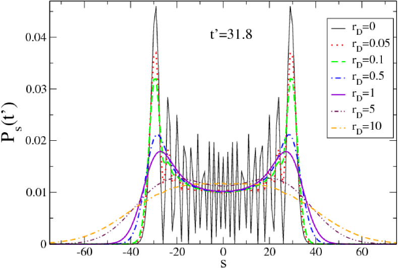
Figure 1: Probability $P_{s}(t^{\prime})$ for an initial condition $\rho(0)=\arrowvert s_{0}\rangle\langle s_{0}\arrowvert$ (where $s_{0}=0$) as a function of position $s$, for $r_{D}=0$, $0.1$, $0.5$, $1$, $5$, $10$ and $t^{\prime}=31.8$, where we have defined the new variables $r_{D}=\frac{2D}{\Omega/\hbar}$ and $t^{\prime}=\frac{\Omega}{\hbar}t$ (dimensionless time).

On the other hand, the quantum purity nielsen ($\mathcal{P}_{Q}(t)\equiv\mbox{Tr}[\rho(t)^{2}]$), a quantity that provides information about whether the state is pure ($\mathcal{P}_{Q}=1$) or mixed ($\mathcal{P}_{Q}<1$), can be calculated analytically. In the present model quantum purity can be calculated using Bessel properties abramowitz ; evangelidis ; martin :

$$\mathcal{P}_{Q}(t) = \mbox{Tr}[\rho(t)^{2}]=\sum_{s_{1}=-\infty}^{\infty}\sum_{s_{3}=-\infty}^{\infty}\langle s_{1}|\rho(t)|s_{3}\rangle\langle s_{3}|\rho(t)|s_{1}\rangle$$

$$= i^{(s_{1}-s_{3})}e^{-2Dt}\!\!\!\!\sum_{n=-\infty}^{\infty}\!\!\!\!J_{s_{1}+n}\!\!\left(\!\frac{\Omega t}{\hbar}\!\right)\!\!J_{s_{3}+n}\!\!\left(\!\frac{\Omega t}{\hbar}\!\right)\!\!I_{n}\!\left(2Dt\right)$$

$$\times i^{(s_{3}-s_{1})}e^{-2Dt}\!\!\!\!\sum_{n^{\prime}=-\infty}^{\infty}\!\!\!\!J_{s_{3}+n^{\prime}}\!\!\left(\!\frac{\Omega t}{\hbar}\!\right)\!\!J_{s_{1}+n^{\prime}}\!\!\left(\!\frac{\Omega t}{\hbar}\!\right)\!\!I_{n^{\prime}}\!\left(2Dt\right).$$

Using the relations $\sum_{n=-\infty}^{\infty}J_{n+m}(x)J_{n+m^{\prime}}(x)=\delta_{m,m^{\prime}}$ and $\sum_{n=-\infty}^{\infty}I_{n}^{2}(x)=I_{0}(2x)$, we get

$$\mathcal{P}_{Q}(t)=e^{-4Dt}I_{0}\left(4Dt\right).$$

The quantum purity takes the value one for $D=0$ (without dissipation) for all time, and for the case $D\neq 0$ the quantum purity takes values smaller than one for $t>0$ (mixed state). For $D\neq 0$, the quantum purity takes on the asymptotic power law behavior $\mathcal{P}_{Q}(t)\sim t^{-1/2}$, for $t\rightarrow\infty$ (using $I_{n}(x)\approx\frac{e^{x}}{\sqrt{2\pi x}}$, for $x\rightarrow\infty$ abramowitz ), in agreement with previous results presented in the references manuel .

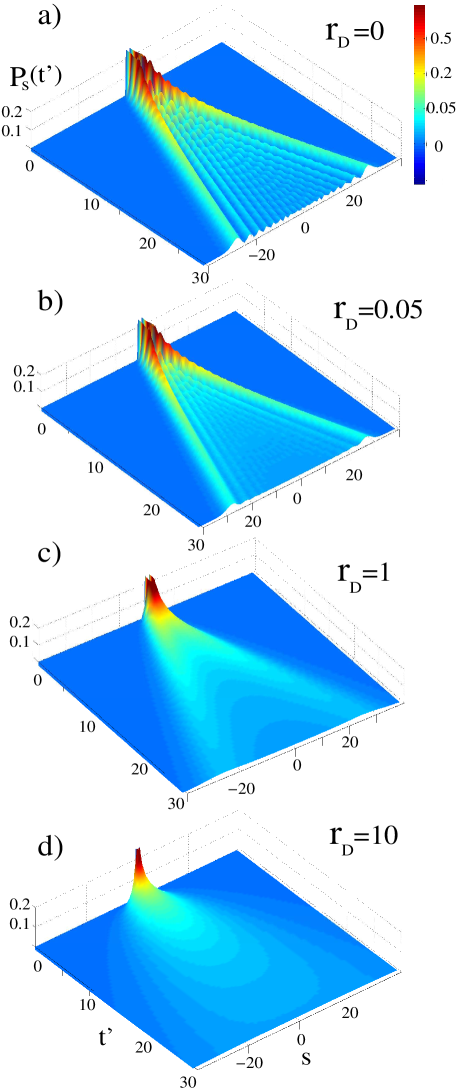
Figure 2: (Color online) Representation in 3D of probability $P_{s}(t^{\prime})$ for an initial condition $\rho(0)=\arrowvert s_{0}\rangle\langle s_{0}\arrowvert$ (where $s_{0}=0$) as a function of position $s$ and $t^{\prime}$, for $r_{D}=0$, $0.05$, $1$, $10$ [(a)-(d)], where the blue regions indicate, approximately, value zero and red regions have high value for probability. The variables $r_{D}$ and $t^{\prime}$ are the same as in Fig.1.

Another important measure that will indicate the presence of quantum behavior is the Wigner function. In the next subsection, we will study this function.

II.2 The Wigner function

The Wigner function was originally formulated as a quasiprobability for the position and momentum of the particle in quantum mechanics. For continuous variables $X$ and $K$, representing position and momentum in the phase space, the Wigner function is given by wigner ; hillery-wigner :

$$W(X,K,t)=\frac{1}{\pi}\int dY\langle X+Y\arrowvert\rho(t)\arrowvert X-Y\rangle e^{2iKY},$$ (17)

where $\rho(t)$ is the time-dependent density operator. The Wigner function could have negative values whereby it is considered a quasi joint probability of $X$ and $K$, and the marginal distribution for $X$ and $K$ can be obtained in the usual form:

$$\int dKW(X,K,t) = \langle X\arrowvert\rho(t)\arrowvert X\rangle,\;\;\;\;\;\;\mbox{(a)}$$

$$\int dXW(X,K,t) = \langle K\arrowvert\rho(t)\arrowvert K\rangle,\;\;\;\;\;\;\mbox{(b)}$$ (18)

where $\langle X\arrowvert\rho(t)\arrowvert X\rangle$ and $\langle K\arrowvert\rho(t)\arrowvert K\rangle$ are the time-dependent probability densities for $X$ and $K$. The normalization condition for $\rho(t)$ can be checked from Eq.(17):

$$\int dX\int dKW(X,K,t)=\mbox{Tr}[\rho(t)]=1.$$ (19)

In our DQW model the space is an infinite one-dimensional regular lattice. Thus, in this case, we propose the Wigner function as:

$$W(s,k,t)=\frac{1}{2\pi}\sum_{s^{\prime}=-\infty}^{\infty}\langle s+s^{\prime}\arrowvert\rho(t)\arrowvert s-s^{\prime}\rangle e^{iks^{\prime}},$$ (20)

where $\arrowvert s\rangle$ is a Wannier basis. This definition fulfills the required conditions for the Wigner function, see Eqs. (18) and (19), using $\sum_{s}$ instead of $\int dX$, where $k\in[-\pi,\pi]$ (first Brillouin zone).

Using Eq.(13) in Eq.(20), we can write the Wigner function as follows:

$$W(s,k,t)\!=\!\frac{e^{-2Dt}}{2\pi}\!\!\!\!\sum_{n,s^{\prime}=-\infty}^{\infty}\!\!\!\!i^{2s^{\prime}}e^{iks^{\prime}}J_{s+s^{\prime}+n}\!\!\left(\!\frac{\Omega t}{\hbar}\!\right)\!\!J_{s-s^{\prime}+n}\!\!\left(\!\frac{\Omega t}{\hbar}\!\right)\!\!I_{n}\!\left(2Dt\right),$$ (21)

then, after some algebra and using Bessel’s properties abramowitz ; evangelidis ; martin ($\sum_{n=-\infty}^{\infty}e^{in\gamma}J_{n+m}(x)J_{n}(x)=J_{m}(2x\sin(\gamma/2))e^{i\beta m}$, where $\beta=\pi/2-\gamma/2$), we find:

$$W(s,k,t)=\frac{e^{-2Dt}}{2\pi}\!\!\!\!\sum_{n=-\infty}^{\infty}\!\!\!\!J_{2s+2n}\!\!\left(2\!\frac{\Omega t}{\hbar}\sin\frac{k}{2}\!\right)\!\!I_{n}\!\left(2Dt\right).$$ (22)

Using Eqs.(18-a) and (18-b) in Eq.(22), we recover the probability densities for position $s$ and momentum $k$ respectively (see, eqs. (14) and (9)).

Interestingly, the Wigner function has information about the transition from DQW to CRW. Analyzing the case $D=0$ (without dissipation in the system) the Wigner function adopts the following form:

$$W(s,k,t)_{QW}=\frac{1}{2\pi}J_{2s}\!\!\left(2\!\frac{\Omega t}{\hbar}\sin\frac{k}{2}\!\right),\;\;\;\;D=0.$$ (23)

In the pure diffusive regimen ($\Omega=0$, i.e., the CRW), the Wigner function can be written as:

$$W(s,k,t)_{CRW}=\frac{e^{-2Dt}}{2\pi}I_{s}\!\left(2Dt\right),\;\;\;\;\Omega=0.$$ (24)

Then from Eqs.(23) and (24), the Wigner function can be re-written as:

$$W(s,k,t)=2\pi\sum_{n=-\infty}^{\infty}W(s+n,k,t)_{QW}\ W(n,k,t)_{CRW},$$

then, changing $n\rightarrow-n$ and considering that $I_{-n}(x)=I_{n}(x)$, we get

$$W(s,k,t)=2\pi\sum_{n=-\infty}^{\infty}W(s-n,k,t)_{QW}\ W(n,k,t)_{CRW},$$ (25)

this expression shows that the Wigner function of the DQW is given in terms of a non-trivial space convolution operation between the QW ($D=0$) and the CRW ($\Omega=0$). For the case $D\neq 0$ this expression shows the nonlocality of the quantum mechanics of a free particle interacting with the quantum thermal $\mathcal{B}$.

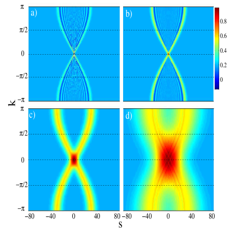
Figure 3: (Color online) Normalized Wigner function $W(s,k,t^{\prime})/W_{max}$ as a function of position $s$ and momentum $k$, for $r_{D}=0$, $0.05$, $1$, $10$ ([(a) $-$ (d)]) and $t^{\prime}=30$, where $W_{max}$ is the maximum value of Wigner function for each value of $r_{D}$. We have considered $r_{D}=\frac{2D}{\Omega/\hbar}$ and $t^{\prime}=\frac{\Omega}{\hbar}t$ (dimensionless). The regions in blue indicate negative values, the ones in sky blue indicate, approximately, zero value and the red regions have the highest values of the Wigner function.

In Fig.3, we show the Wigner function from Eq.(22) or Eq.(25). We have normalized the Wigner function with respect to its maximum value $W_{max}$ for each value of $r_{D}$ (i.e.: we use $W(s,k,t^{\prime})/W_{max}$, where $t^{\prime}=\frac{\Omega}{\hbar}t$ and $r_{D}=\frac{2D}{\Omega/\hbar}$). Similar Wigner’s quantum carpets have been analyzed for a QW on a ring without dissipation in blumen3 . In Fig.3(a), we observe the quantum behavior for $r_{D}=0$. In this case the Wigner function has negative and positive values, and it shows remarkable oscillatory behavior (see Eq.(23)). In the case of small values of the dissipation, $r_{D}<<1$, we observe (Fig.3(b), with $r_{D}=0.05<<1$) that the oscillatory behavior starts to diminish and for values of $r_{D}\gtrsim 1$ (fig 3(c)-(d)) the dissipative term is dominant. In this case, the Wigner function takes only positive values, therefore it is a well-defined joint probability, and the system resembles a CRW when $r_{D}$ tends to infinity. In this case, the system is diffusive (see Eq.(24)).

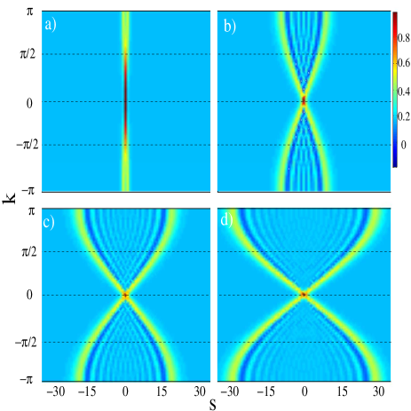
Figure 4: (Color online) Normalized Wigner function $W(s,k,t^{\prime})/W_{max}$ as a function of position $s$ and momentum $k$, for $t^{\prime}=1$, $10$, $20$, $30$ ([(a) $-$ (d)]) and $r_{D}=0.05$, in this case $W_{max}$ is the maximum value of Wigner function for each value of $t^{\prime}$.

In a complementary way, we now show the Wigner function (similar to Fig 3), but we have fixed the parameter $r_{D}=0.05$ and changed the dimensionless time $t^{\prime}$. In Fig.4[(a)-(d)], we observe the Wigner function for $t^{\prime}=1$, $10$, $20$, $30$. The time-evolution of the Wigner function also shows the transition from the DQW to the CRW.

In order to define a criterion to indicate when quantum correlations dominate over the classical correlations, or vice versa, we show in Fig.5 the Wigner function $W_{0}=W(0,\pi,t^{\prime})$, as function of time $t^{\prime}$. We note an oscillatory behavior of $W_{0}$ for $r_{D}<1$. In the inset of Fig.5, we show the Wigner function $W_{1}=W(0,\pi,1.9)$ as a function of $r_{D}$ (we consider the value of $t^{\prime}$ where $W_{0}$ takes their first minimum). We use this as a criterion to indicate when quantum correlations are more important than classical correlations, and from Fig.5, we note that for $r_{D}\lesssim r_{D}^{c}$, with $r_{D}^{c}=0.52$, the Wigner function is $W_{0}<0$, therefore, the quantum correlations dominate in the system. For the case when $r_{D}>r_{D}^{c}$, the Wigner function is non-negative for all parameters in the system. In this case the classical correlations dominate over the quantum correlations. Therefore, in this situation, we could say that the Wigner function is a joint probability density in the phase space (because $W(s,k,t)\geq 0$). This criterion is not unique, other criteria could be used.

These results are consistent with the previous results obtained with the probability of finding the particle in the lattice site (see Figures 1-2).

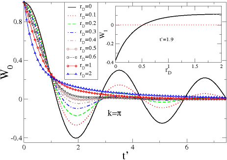
Figure 5: The Wigner function $W_{0}=W(0,\pi,t^{\prime})$, as a function of time $t^{\prime}$, for $r_{D}=0$, $0.1$, $0.2$, $0.3$, $0.4$, $0.5$, $0.6$, $1$, $2$. The Wigner function $W_{1}=W(0,\pi,1.9)$, as a function of $r_{D}$, see inset. For $r_{D}\gtrsim 0.52$ the Wigner function is non-negative, and well defined as a joint probability density in the phase space.

II.3 The long-time limit of the reduced density matrix

In this subsection, we have analyzed the long-time limit behavior of the reduced density matrix. The Eq.(II.1) can be written in the form:

$$\left\langle s_{1}\right|\rho(t)\left|s_{2}\right\rangle=\int_{-\pi}^{\pi}\frac{dk_{1}}{2\pi}e^{i\frac{\Omega t}{\hbar}\cos k_{1}}\mathcal{I}(k_{1}),$$ (26)

where

$$\mathcal{I}(k_{1})\!\!=\!\!\!\int_{-\pi}^{\pi}\!\!\frac{dk_{2}}{2\pi}e^{-i\frac{\Omega t}{\hbar}\!\cos k_{2}}\!\cos\left[\left(k_{1}\!\!-\!\!k_{2}\right)\!(s_{1}\!\!-\!\!s_{2})\right]e^{2Dt\left(\cos(k_{1}\!-\!k_{2})\!-\!1\right)},$$ (27)

By symmetry the term proportional to $\sin\left[\left(k_{1}-k_{2}\right)(s_{1}-s_{2})\right]$ cancels out. Noting that in the long-time limit $\mathcal{I}(k_{1})$ can be calculated by using the stationary phase approximation MSP , we get (in the limit: $\Omega/\hbar>>2D$ and $t\rightarrow\infty$)

$$\mathcal{I}(k_{1}) \simeq \sqrt{\frac{2\pi}{\Omega t}}\left\{e^{-2Dt(1-\cos k_{1})-i(\Omega t-\pi/4)}\cos k_{1}s_{1}\right.$$

$$\left.+e^{-2Dt(1+\cos k_{1})+i(\Omega t-\pi/4)}\cos(k_{1}s_{1}-\pi s_{2})\right\}.$$

Introducing this expression in Eq.(26) we can apply once again the stationary phase approximation (taking care that the saddle point $(0,0)$ in the bi-dimensional integration does not contribute), then for the reduced density matrix in the asymptotic limit ($(\Omega/\hbar)t\rightarrow\infty$) we get:

$$\langle s_{1}|\rho(t)|s_{2}\rangle\! \rightarrow \!\frac{2\hbar}{\pi\Omega t}\{\cos\pi(s_{1}+s_{2})+\cos\pi(s_{1}-s_{2})$$

$$+e^{-4Dt}[\sin(2\frac{\Omega}{\hbar}t)\cos(s_{1}+s_{2})\frac{\pi}{2}\cos(s_{1}-s_{2})\frac{\pi}{2}]$$

$$-ie^{-4Dt}[\cos(2\frac{\Omega}{\hbar}t)\sin(s_{1}+s_{2})\frac{\pi}{2}\sin(s_{1}-s_{2})\frac{\pi}{2}]\}.$$

This result is in agreement with the asymptotic approximation of the Bessel function when it is replaced in the Eq.(13) (for $x\rightarrow\infty$, $J_{n}(x)\approx\sqrt{\frac{2}{\pi x}}\cos(x-\frac{\pi}{4}-n\frac{\pi}{2})$). Thus we see that for long-time, terms proportional to $e^{-4Dt}$ will contribute to the quantum entropy production associated with the reduced density matrix. In fact, this contribution is proportional to the following matrix (in Wannier representation):

$$\begin{array}[]{cc}&\!\!\!\!\!\!\!\!\cdots\cdots\cdots-1,\;\;\;0,\;\;+1\cdots\cdots\cdots\cdots\\ \begin{array}[]{c}\vdots\\ \vdots\\ \vdots\\ -1\\ \,\,\,\,0\\ +1\\ \vdots\\ \vdots\\ \vdots\end{array}&\left(\begin{array}[]{cccccccccc}\ddots&\cdot&\cdot&\cdot&\cdot&\cdot&\cdot&\cdot&\cdot&\cdot\\ \cdot&A&-iB&A&-iB&A&-iB&A&\cdot&\\ \cdot&iB&A&iB&A&iB&A&iB&\cdot&\\ \cdot&A&-iB&A&-iB&A&-iB&A&\cdot&\\ \cdot&iB&A&iB&A&iB&A&iB&\cdot&\\ \cdot&A&-iB&A&-iB&A&-iB&A&\cdot&\\ \cdot&iB&A&iB&A&iB&A&iB&\cdot&\\ \cdot&A&-iB&A&-iB&A&-iB&A&\cdot&\\ \cdot&\cdot&\cdot&\cdot&\cdot&\cdot&\cdot&\cdot&\cdot&\ddots\end{array}\right),\end{array}$$ (29)

where $A=\frac{2\hbar}{\pi\Omega t}(1-\sin(2\Omega t/\hbar)e^{-4Dt})$, $B=\frac{2\hbar}{\pi\Omega t}\cos(2\Omega t/\hbar)e^{-4Dt}$. This means that asymptotically the probability profile $\rho_{ss}(t)$ goes to zero uniformly in the lattice, similar to $\sim\frac{2\hbar}{\pi\Omega t}(1-\sin(2\Omega t/\hbar)e^{-4Dt}$, and the off-diagonal elements form a time-dependent coherent binary structure of $\left\{A,\pm iB\right\}$ (in the Wannier representation) that also goes to zero asymptotically as $\sim 1/t$. Due to the fact that Anderson’s boundaries move at finite velocity $V_{A}=\frac{1}{\sqrt{2}}\frac{\Omega}{\hbar}$ away from the initial condition (state $\left|s_{0}\right\rangle\left\langle s_{0}\right|$), we expect that the DQW will be always inside a (time-dependent) finite domain of maximum size $L\sim\sqrt{\left\langle\mathbf{q}(t)^{2}\right\rangle-\left\langle\mathbf{q}(t)\right\rangle^{2}}>>\epsilon$ ($\epsilon$ is the lattice parameter, we take $\epsilon=1$), which increases linearly in time. Then, we can calculate the asymptotic eigenvalues of $\left\langle s_{1}\right|\rho(t)\left|s_{2}\right\rangle$ by approximating $\rho(t)$ to be a $L\times L$ finite-domain matrix.

It is simple to calculate the non-null eigenvalues of a matrix of dimension $L\times L$ of the form (29). For $D=0$ (without dissipation) there is only one non-null eigenvalue:

$$\lambda=\frac{2\hbar}{\pi\Omega t}[L-\sin(2\frac{\Omega}{\hbar}t)].$$ (30)

On the other hand, for the case $D\neq 0$, but $\Omega/\hbar>>2D$, we obtain only two non-null eigenvalues for the reduced density matrix. These eigenvalues are as follows:

$$\lambda_{\pm} = \frac{2\hbar}{\pi\Omega t}\{L-\sin(2\frac{\Omega}{\hbar}t)$$

$$\pm\sqrt{1\!+\!(L^{2}\!-\!1)e^{-8Dt}\!-\!2Le^{-4Dt}\sin(2\frac{\Omega}{\hbar}t)\!+\!e^{-8Dt}\sin^{2}(2\frac{\Omega}{\hbar}t)}\}.$$

As expected, we observe from this expression that if we take $D=0$, we recover the Eq.(30). These results allow us to calculate the long-time behavior of the von Neumann entropy.

III Quantum entanglement in the DQW

III.1 Time evolution of von Neumann’s Entropy

In order to study the irreversibility behavior of a free particle in interaction with a quantum thermal bath $\mathcal{B}$, i.e., our DQW model, we have calculated von Neumann’s entropy corresponding to non-equilibrium situations, assuming that the system is prepared in a highly localized state (i.e., we adopt the initial condition $\rho(0)=\left|s_{0}\right\rangle\left\langle s_{0}\right|$, with $s_{0}=0$).

$$\mathcal{S}(t)=-\mbox{Tr}\left[\rho(t)\ln\rho(t)\right].$$ (32)

In an open quantum system the reduced density matrix evolves in a Markovian approximation, following the QME (Eq.(2)). Due to the dissipation, the reduced density matrix $\rho(t)$ will not be diagonal at any time $t>0$. The information of the quantum entanglement between the quantum thermal bath and our free particle -in the lattice- can be obtained from the reduced density matrix given in the Eq.(13). Due to the fact that the total system is a pure state, the von Neumann entropy for the reduced density matrix can be used to measure the entanglement. Then we should calculate von Neumann’s entropy numerically using $\rho(t)$ in the Wannier base. We have fixed the size of the chain to be $L$, with $L\approx V_{A}t$ where $V_{A}=\frac{1}{\sqrt{2}}\frac{\Omega}{\hbar}$, thus we have diagonalized the reduced density matrix. Then we can use the following expression for the quantum entropy:

$$\mathcal{S}(t)=-\sum_{i}\Lambda_{i}\ln\Lambda_{i},$$ (33)

where $\Lambda_{i}$ is an eigenvalue of the reduced density matrix $\langle s_{1}\arrowvert\rho(t)\arrowvert s_{2}\rangle$ in the domain $\left[-L,L\right].$ We expect that for finite times (even in an infinite lattice) $\mathcal{S}(t)\neq\infty.$ We have carried out this calculation numerically and we have shown in Fig.6 $\mathcal{S}(t)$ as a function of time $t^{\prime}=\frac{\Omega}{\hbar}t$ for different values of the dissipative parameter $r_{D}=\frac{2D}{\Omega/\hbar}$.

In Fig.6(a), we observe the quantum entropy as function of $r_{D}$ and $t^{\prime}$ (3D visualization). As expected for $r_{D}=0$ ($D=0$), the quantum entropy is $\mathcal{S}(t^{\prime})=0$ for all $t^{\prime}\geq 0$. In this case the quantum entanglement between the free particle in the lattice and the phonon bath is zero, which means we can write the wave function of the total system as a product of one state of the free particle in the lattice and one of the phonon bath (separable state). Another trivial result is the case that $t^{\prime}=0$, where the quantum entropy is zero for $r_{D}\geq 0$ (in this case $\rho(t^{\prime}=0)=\arrowvert s_{0}\rangle\langle s_{0}\arrowvert$). In the presence of dissipation the total system is no longer a separable state between the particle in the lattice and environment. The reduced density matrix $\rho(t)$ is a mixed state (for $D>0$), and the quantum entropy starts increasing in time for a fixed value of $r_{D}$. We also note that for a fixed value of $t^{\prime}$, the magnitude of the quantum entropy increases as $r_{D}$ increases. The quantum entropy gives information about the transition from the DQW to the CRW, which is consistent with the results obtained above concerning the probability profile and the Wigner function. Finally, in Fig.6(b), we show results of the quantum entropy as a function of $t^{\prime}$ and different values of $r_{D}$.

Similar analyses to measure quantum correlations have been carried out by considering a free particle (in a lattice) with an additional internal degree of freedom: the quantum ”coin”. Thus, the correlation between the coin and the spatial degree of freedom have been studied in detail, and these models share some similarities with our results despite the fact that by considering the quantum coin as the thermal bath, the latter has a finite Hilbert space chandrashekar ; Romanelli2 .

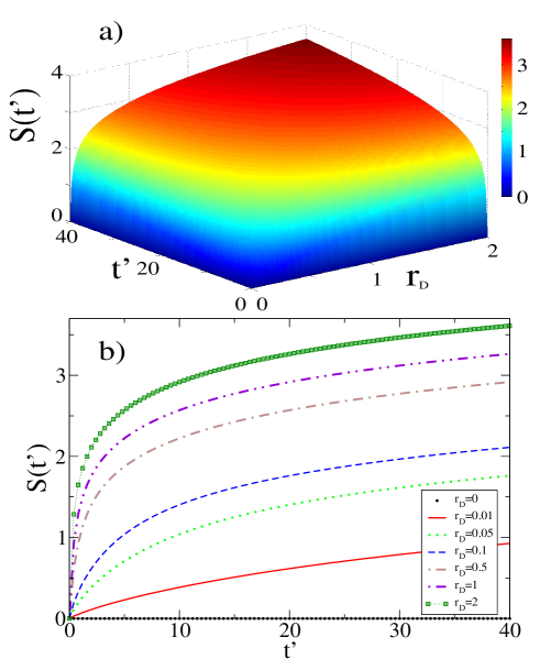
Figure 6: (Color online) von Neumann’s entropy as a function of $t^{\prime}$ and $r_{D}$ (Fig (a)). This function measures the quantum entanglement between the particle in the lattice and the phonons bath. We show a plot in 2D (Fig. (b)) of quantum entropy as a function of $t^{\prime}$ for different values of $r_{D}=0$, $0.01$, $0.05$, $0.1$, $0.5$, $1$, $2$.

Interestingly, by introducing the stationary phase approximation in Eq.(II.1), it is possible to obtain asymptotic behavior for $\left\langle s_{2}\right|\rho(t)\left|s_{1}\right\rangle$, then we can study the time-dependence of $\mathcal{S}(t)$ in the long-time regime analytically.

III.1.1 The long-time limit of von Neumann’s entropy

Having the result of Eq.(II.3) we can re-write von Neumann’s entropy in the long-time regime in the form:

$$\mathcal{S}(t) = -\sum_{s_{1}=-\infty}^{\infty}\sum_{s_{2}=-\infty}^{\infty}\!\!\!\!\left\langle s_{1}\right|\rho(t)\left|s_{2}\right\rangle\left\langle s_{2}\right|\ln\rho(t)\left|s_{1}\right\rangle$$ (34)

$$\simeq -\sum_{j=1}^{L}\lambda_{j}\ln\lambda_{j},$$

here $\lambda_{j}$ are the eigenvalues associated with the asymptotic long-time regime of the reduced density matrix $\left\langle s_{1}\right|\rho(t)\left|s_{2}\right\rangle$. Using Eq.(II.3) in Eq.(34) and considering $L>>1$ (for simplicity, we re-normalized the eigenvalues of $\rho(t)$); we get (when $\frac{\Omega}{\hbar}>>2D$ and $\frac{\Omega}{\hbar}t>>1$):

$$\mathcal{S}(t)\!\! \simeq -(\frac{1-e^{-4Dt}}{2})\ln(\frac{1-e^{-4Dt}}{2})$$ (35)

$$- (\frac{1+e^{-4Dt}}{2})\ln(\frac{1+e^{-4Dt}}{2}).$$

In addition, another asymptotic approximation to $\mathcal{S}(t)$ can be made if we consider $D\sim 0$ (with $Dt<<1$ ), so we can approximate $e^{-4Dt}\rightarrow 1-4Dt$ and replacing this expression in Eq.(35) we get a simpler expression for the quantum entropy in the form:

$$\mathcal{S}(t)\simeq-2Dt\ln(2Dt),\quad Dt<<1.$$

Note that in the limit $D\rightarrow 0$ (even when $t\gg 1$) the quantum entropy $\mathcal{S}(t)\rightarrow 0$. We have checked this analytical result with our numerical calculation using Eq.(33) and the agreement is excellent, see Fig.6.

IV Conclusions

A free particle -in an infinite regular lattice- in interaction with a thermal phonon bath has been studied by tracing out the degree of freedom of the bath. We then worked out the quantum master equation for a dissipative tight-binding model.

We have solved the master equation analytically by using Bessel functions, and obtained the reduced density matrix $\rho(t)$ as a function of the scale energies of the system ($\Omega/\hbar$, $D$). We have also studied the transition from Dissipative Quantum Walk to Classical Random Walk in terms of parameters $D$ and $\Omega/\hbar$ (or $r_{D}=\frac{2D}{\Omega/\hbar}$). In the case when $2D<<\Omega/\hbar$ ($r_{D}<<1$) the quantum behavior is more important than the dissipation in the system. In the opposite case we re-obtain the Classical Random Walk $2D>>\Omega/\hbar$ ($r_{D}>>1$) because in this case the dissipation creates decoherence in the system. We have studied the Wigner function to analyze the pseudo-probability densities in the phase space. This function is very useful as an indicator of this quantum-classical transition.

As an alternative approach to the study of the transition from Dissipative Quantum Walk to Classical Random Walk we have used tools from quantum information theory (as a function of dissipative parameter) to analyze the reduced density matrix. To describe this transition we have used von Neumann’s entropy $\mathcal{S}(t)$ to measure the quantum entanglement between the free particle -in a lattice- and the phonon bath. We observed that for $D=0$ the quantum entropy is $\mathcal{S}(t^{\prime})=0$ for $t^{\prime}\geq 0$ (closed system), and when $D$ increases we show that quantum decoherence starts to appear and therefore the quantum entropy increases in time with a law which is slower than that from classical statistics ($\mathcal{S}(t)_{CRW}\sim\ln t$) Caceres (2003); Kampen . Asymptotically for $D\rightarrow 0$ the quantum entropy turns out to be only a function of the dissipative parameter $D$. This fact also indicates the beginning of the transition from the Dissipative Quantum Walk to the Classical Random Walk.

This analytical model allows us to study the effect of decoherence in the Dissipative Quantum Walk as a function of the two typical energies of the system. We can conclude that in the present model there are two characteristic time scales: the dissipative time $\tau_{D}\sim 1/D$ and the hopping time $\tau_{H}\sim\hbar/\Omega$; the competition between these time scales controls the decoherence and correlation mechanism in the system. For example, the quantum purity $\mathcal{P}_{Q}(t)$ is controlled by $\tau_{D}$, but in general the entropy and the interference phenomena appearing in the probability profile or in the Wigner phase-space pseudo-distribution are controlled by the competition between these time scales.

The interesting problem of the propagation of photons in waveguide lattices are possible scenarios where our present results can be applied, also the analysis of the entanglement of a bipartite system can be studied in the present framework, works along these lines are in progress. In this way the present model gives insight into the effect of dissipation in more complex quantum systems, for instance, the analysis of quantum correlations between two particles -in a regular lattice- in interaction with a phonon bath.

Acknowledgments. We thank Maria del Carmen Ferreiro for the English revision of the manuscript. M.O.C gratefully acknowledges support received for this study from Universidad Nacional de Cuyo, Argentina, project SECTyP, and CONICET, Argentina, grant PIP 90100290. M.N. gratefully acknowledges CONICET, Argentina for his Post-Doctoral fellowship.

Appendix A On the second quantization and the one-particle tight-binding Hamiltonian

A free Hamiltonian in the tight-binding approximation for spinless particles (fermion) can be written in second quantization in the form haken :

$$H_{S}=E_{0}\sum_{s_{=}{-\infty}}^{\infty}c_{s}^{{\dagger}}c_{s}-\frac{\Omega}{2}\left(\sum_{s_{=}{-\infty}}^{\infty}c_{s-1}^{{\dagger}}c_{s}+c_{s+1}^{{\dagger}}c_{s}\right),$$ (36)

where $c_{s}^{{\dagger}}$ and $c_{s}$ are creation and destruction operators in the site $s$ of the lattice respectively ($\arrowvert\cdots,0,1_{s},0,\cdots\rangle=c_{s}^{{\dagger}}\arrowvert 0\rangle$, where $\arrowvert 0\rangle$ is the empty state). Then considering only one particle it is straightforward to compare Eq.(36) with $H_{S}$ in Eq.(1), if we replace $a$ and $a^{{\dagger}}$ with a combination of $c_{s^{\prime}}^{{\dagger}}$ and $c_{s^{\prime}}$, in the following way:

$$a\Rightarrow R=\sum_{s_{=}{-\infty}}^{\infty}c_{s-1}^{{\dagger}}c_{s},\;\;\;a^{{\dagger}}\Rightarrow R^{{\dagger}}=\sum_{s_{=}{-\infty}}^{\infty}c_{s+1}^{{\dagger}}c_{s},$$ (37)

where $c_{s}$ are acting in the Fock-space. Therefore, we can also check that $R$ and $R^{{\dagger}}$ commute in the general case for many particles (where $R^{{\dagger}}R=RR^{{\dagger}}=\sum_{s_{=}{-\infty}}^{\infty}c_{s}^{{\dagger}}c_{s}-\sum_{s,s_{=}^{\prime}{-\infty}}^{\infty}c_{s+1}^{{\dagger}}c_{s^{\prime}-1}^{{\dagger}}c_{s}c_{s^{\prime}}$), and for one particle in the lattice we get $RR^{{\dagger}}=\mathbf{1}$.

Equation (37) shows the expected mapping from Fock’s space into the Winner basis. Then the connection between the tight-binding Hamiltonian and the QW model can be established.

Appendix B Reduced matrix density

Here we show how to obtain Eq.(13). Replacing the following relations for the Bessel function: $e^{iz\cos\theta}=\sum_{n=-\infty}^{\infty}i^{n}J_{n}(z)e^{in\theta}$; $e^{z\cos\theta}=\sum_{n=-\infty}^{\infty}I_{n}(z)e^{in\theta}$ in Eq.(II.1), where $J_{n}$ and $I_{n}$ are a Bessel functions of integer order abramowitz ; evangelidis , we find:

$$\langle s_{1}|\rho(t)|s_{2}\rangle \!\!\!\!=\!\!\!\! \left(\!\frac{1}{2\pi}\!\right)^{\!\!2}e^{-2Dt}\!\!\!\!\!\!\!\!\!\sum_{m_{1},m_{2},n=-\infty}^{\infty}\!\!\!\!\!\!\!\!J_{m_{1}}\!\!\left(\!\frac{\Omega t}{\hbar}\!\right)\!\!J_{m_{2}}\!\!\left(\!\frac{\Omega t}{\hbar}\!\right)\!\!I_{n}\!\left(2Dt\right)$$

$$\times i^{m_{1}+m_{2}}\!\!\int_{-\pi}^{\pi}\!\!\!\!dk_{1}e^{i(s_{1}+m_{2}+n)k_{1}}\!\!\int_{-\pi}^{\pi}\!\!\!\!dk_{2}e^{-i(s_{2}-m_{1}+n)k_{2}}.$$

Using the definition of Kronecker delta: $\delta_{s,s^{\prime}}=\frac{1}{2\pi}\int_{-\pi}^{\pi}e^{ik(s-s^{\prime})}$ in the previous expression, we finally obtain:

$$\langle s_{1}|\rho(t)|s_{2}\rangle\!\!=\!i^{(s_{1}-s_{2})}e^{-2Dt}\!\!\!\!\!\sum_{n=-\infty}^{\infty}\!\!\!\!J_{s_{1}+n}\!\!\left(\!\frac{\Omega t}{\hbar}\!\right)\!\!J_{s_{2}+n}\!\!\left(\!\frac{\Omega t}{\hbar}\!\right)\!\!I_{n}\!\left(2Dt\right).$$

Appendix C Moments of the position operator - The characteristic function

We have defined a characteristic function Kampen for calculating moments of position operator $\mathbf{q}$ in the following way:

$$\mathcal{G}(\xi)=\mbox{Tr}[\rho(t)e^{i\xi\mbox{{\bf q}}}]=\sum_{l=-\infty}^{\infty}\langle l\arrowvert\rho(t)\arrowvert l\rangle e^{i\xi l},$$ (38)

thus the quantum moments of $\mathbf{q}$ can be obtained using the following expression:

$$\langle\mbox{{\bf q}}(t)^{m}\rangle=\frac{1}{i^{m}}\frac{d^{m}}{d\xi^{m}}\mathcal{G}(\xi)\biggl{|}_{\xi=0},$$ (39)

Using Eq.(13) in Eq.(38), we can write the characteristic function in the form:

$$\mathcal{G}(\xi)=e^{-2Dt\left(1-\cos\xi\right)}\ J_{0}\left(2t\frac{\Omega}{\hbar}\sin\frac{\xi}{2}\right),$$ (40)

here we have said that $\sum_{n=-\infty}^{\infty}e^{in\gamma}J_{n+m}(x)J_{n}(x)=J_{m}(2x\sin(\gamma/2))e^{i\beta m}$, where $\beta=\pi/2-\gamma/2$. From this characteristic function all the moments of the position operator can be calculated straightforwardly. In particular, we can re-obtain the variance of the DQW (see Eq.(7)). Note that in the classical limit $\Omega=0$ we recover the expected characteristic function associated with the CRW Kampen ; Caceres (2003). In general, Eq. (40) shows that the non-equilibrium behavior of the characteristic function of the DQW is the product of the classical one and the quantum characteristic function $J_{0}\left(2t\frac{\Omega}{\hbar}\sin\frac{\xi}{2}\right)$.

References

- (1) C. Kittel, Introduction to Solid State Physics (Wiley, New York, 1986).
- (2) M. Nielsen and I. Chuang, Quantum Computation and Quantum Information (Cambridge University Press, Cambridge, 2000).
- (3) R. Alicki and Lendi K. Quantum Dynamical Semigroups and Applications (Lectures Notes in Physics, Vol. 286, Berlin, Springer, 1987).
- (4) U. Weiss, Quantum dissipation systems, (World Scientific, Singapore, 2008).
- (5) C.W. Gardiner, Quantum Noise (Springer, Berlin, 1991).
- (6) N.G. van Kampen, Stochastic Processes in Physics and Chemistry, 2a ed. (North Holland, Amsterdam, 1992).
- (7) F. Zähringer, G. Kirchmair, R. Gerritsma, E. Solano, R. Blatt, and C. F. Roos, Phys. Rev. Lett. 104, 100503 (2010).
- (8) N. W. Ashcroft, N. D. Mermin, Solid State Physics, Saunders College (1976).
- (9) A. Schreiber, K. N. Cassemiro, V. Potoček, A. Gábris, I. Jex, and Ch. Silberhorn, Phys. Rev. Lett. 106, 180403 (2011).
- (10) Yue Yin, D. E. Katsanos, and S. N. Evangelou, Phys. Rev. A 77, 022302 (2008).
- (11) Y. Aharonov, L. Davidovich, and N. Zagury, Phys. Rev. A 48, 1687 (1993).
- (12) N.G. van Kampen; J. Stat. Phys. 78, 299 (1995).
- (13) J. Kempe, Contemp. Phys. 44, 307 (2003).
- (14) D. E. Katsanos, S. N. Evangelou, and S. J. Xiong, Phys. Rev. B 51, 895 (1995).
- (15) M. Esposito and P. Gaspard, Phys. Rev. B 71, 214302 (2005).
- (16) N. Konno, Quant. Inf. Proc. 8, 387 (2009).
- (17) Balaji R. Rao and R. Srikanth, C. M. Chandrashekar and Subhashish Banerjee, Phys. Rev. A 83, 064302 (2011); C. M. Chandrashekar, R. Srikanth, and S. Banerjee, Phys. Rev. A 76, 022316 (2007); R. Srikanth, S. Banerjee, and C. M. Chandrashekar, Phys. Rev. A 81, 062123 (2010).
- (18) A. Romanelli, Phys. Rev. A, 76, 054306 (2007).
- (19) M. A. Broome, A. Fedrizzi, B. P. Lanyon, I. Kassal, A. Aspuru-Guzik and A. G. White, Phys. Rev. Lett. 104, 153602 (2010).
- (20) D. Shapira, O. Biham, A. J. Bracken and M. Hackett, Phys. Rev A 68, 062315 (2003).
- (21) W. Dür, R. Raussendorf, V. M. Kendon and H-J Briegel, Phys. Rev. A 66, 052319 (2002).
- (22) A. Joye and M. Merkli, J. Stat. Phys. 140, 1 (2010).
- (23) H. Schmitz, R. Matjeschk, Ch. Schneider, J. Glueckert, M. Enderlein, T. Huber, and T. Schaetz, Phys. Rev. Lett. 103, 090504 (2009).
- (24) H. B. Perets, Y. Lahini, F. Pozzi, M.Sorel, R. Morandotti, and Y. Silberberg, Phys. Rev. Lett. 100, 170506 (2008).
- (25) Peruzzo et al., Science 329, 1500 (2010).
- (26) Cáceres M O and Chattah A K J. Mol. Liq. 71, 187 (1997).
- (27) Oliver Mülken and Alexander Blumen, Phys. Rev. E, 71, 036128 (2005).
- Caceres (2003) M.O. Cáceres, (in Spanish) Elementos de estadística de no equilibrio y sus aplicaciones al transporte en medios desordenados, Reverté S.A., Barcelona, (2003).
- (29) F. Bardou, J. Ph. Bouchaud, A. Aspect, and C. Cohen-Tannoudji, Lévy Statistics and Laser Cooling, Cambridge University Press, (Cambridge, 2003).
- (30) G. Margolin, V. Protasenko, M. Kuno, and E. Barkai, J. Phys. Chem. B, 110, 19053, (2006).
- (31) V. Kendon, Math. Struct. in Comp. Sci 17, 1169 (2006).
- (32) V. Gorini and A. Kossakowski; J. Math. Phys. 17, 821 (1976).
- (33) G. Lindblad, Commun. Math. Phys. 48, 119 (1976).
- (34) R.P. Feynmann, F.L. Vernon, and R.W. Hellwarth, J. Appl. Phys. 28, 49, (1957).
- (35) R.P. Feynmann, F.L. Vernon, An. of Phys. 24, 118, (1963).
- (36) A.O. Caldeira and A.J. Legget; Ann. Phys. (USA), 149, 374, (1983).
- (37) M.B. Plenio, P.L. Knight; Rev. Mod. Phys, 70, 101 (1998).
- (38) K. Blum, Density Matrix Theory and Applications (Plenum Press, New York, 1981).
- (39) H. Spohn; Rev. Mod. Phys. 52, 569 (1980); R. Dumcke, H. Spohn, Z. Phys. B, 34, 419, (1979).
- (40) J. D. Whitfield, César A. Rodríguez-Rosario, and Alán Aspuru-Guzik, Phys. Rev. A 81, 022323 (2010).
- (41) M. O. Cáceres and M. Nizama, J. Phys. A: Math. Theor. 43 455306 (2010).
- (42) A.A. Budini, A.K. Chattah and M.O. Cáceres; J. Phys. A Math. and Gen. 32, 631 (1999).
- (43) A.K. Chattah and M.O. Cáceres, Cond. Matt. Phys. 3, 51 (2000).
- (44) M. Abramowitz and I. A. Stegun, Handbook of Mathematical Functions, Dover Publications, Nueva York (1995).
- (45) E. A. Evangelidis, J. Math. Phys. 25, 2151 (1984).
- (46) P. A. Martin, J. Phys. A: Math. Theor. 41 015207 (2008).
- (47) E. P. Wigner, Phys. Rev. 40, 749 (1932).
- (48) M. Hillery, R. F. O’Connell, M. O. Scully, and E. P. Wigner, Phys. Rep. 106, 121 (1984).
- (49) Oliver Mülken and Alexander Blumen, Phys. Rev. A, 73, 036105 (2006).
- (50) N.G. van Kampen, Physica 24, 437 (1958).
- (51) A. Romanelli, Phys. Rev. A 85, 012319 (2012).
- (52) H. Haken, Quantum Field Theory of Solids, (North-Holly, Amsterdam, 1976).