Properties of neutral mesons in a hot and magnetized quark matter

Abstract

The properties of noninteracting $\sigma$ and $\pi^{0}$ mesons are studied at finite temperature, chemical potential and in the presence of a constant magnetic field. To do this, the energy dispersion relations of these particles, including nontrivial form factors, are derived using a derivative expansion of the effective action of a two-flavor, hot and magnetized Nambu–Jona-Lasinio (NJL) model up to second order. The temperature dependence of the pole and screening masses as well as the directional refraction indices of magnetized neutral mesons are explored for fixed magnetic fields and chemical potentials. It is shown that, because of the explicit breaking of the Lorentz invariance by the magnetic field, the refraction index and the screening mass of neutral mesons exhibit a certain anisotropy in the transverse and longitudinal directions with respect to the direction of the external magnetic field. In contrast to their longitudinal refraction indices, the transverse indices of the neutral mesons are larger than unity.

I Introduction

The study of the states of quark matter under extreme conditions has attracted much attention over the past few years. Extreme conditions include high temperatures and finite baryonic chemical potentials as well as strong magnetic fields. The latter is responsible for many interesting effects on the properties of quark matter. Some of the most important ones are magnetic catalysis of dynamical chiral symmetry breaking klimenko1992 ; miransky1995 ; catalysis , that leads to a modification of the nature of electroweak ayala2008 , chiral and color-superconducting phase transitions superconducting ; fayazbakhsh2010-1 ; fayazbakhsh2010 ; skokov2011 ; pawlowski2012 , production of chiral density waves klimenko2010 , chiral magnetic effect kharzeev2008 , and last but not least inducing electromagnetic superconductivity and superfluidity chernodub2011 . In this paper, we will focus on the effect of constant magnetic fields on the properties of neutral and noninteracting mesons in a hot and dense quark matter. In particular, the temperature dependence of meson masses as well as their direction-dependent refraction indices and screening masses will be explored in the presence of various fixed magnetic fields. The largest observed magnetic field in nature is about $10^{12}-10^{13}$ Gauß in pulsars and up to $10^{14}-10^{15}$ Gauß on the surface of some magnetars, where the inner field is estimated to be of order $10^{18}-10^{20}$ Gauß incera2010 . There are also evidences for the creation of very strong and short-living magnetic fields in the early stages of non-central heavy ion collisions at RHIC kharzeev51-STAR ; mclerran2007 . Depending on the collision energies and impact parameters, the magnetic fields produced at RHIC and LHC are estimated to be in the order $eB\sim 1.5~{}m_{\pi}^{2}$, corresponding to $0.03$ GeV² for $m_{\pi}=138$ MeV, and $eB\sim 15~{}m_{\pi}^{2}$, corresponding to $0.3$ GeV², respectively skokov2010 . On the other hand, it is known that the quark-gluon plasma, produced in high-energy heavy-ion collisions, passes over many stages during its evolution. The last of which consists of a large amount of hadrons, including pions, until a final freeze-out ayala2002 . Thus, the presence of a background magnetic field created in heavy ion experiments may affect the properties of “charged quarks” in the earliest stage of the collision and although the created strong magnetic field is extremely short living and decays very fast mclerran2007 ; skokov2010 , it may affect the properties of the hadrons made of these “magnetized” quarks. Even the properties neutral mesons may be affected by the external magnetic field produced in the earliest phase of heavy-ion collisions. In the present paper, we do not intend to go through the phenomenology of heavy-ion collisions. Our computation is only a theoretical attempt to study the effect of external magnetic fields on “magnetized” neutral mesons, that, because of the lack of electric charge, do not interact directly with the external magnetic field. Our study is indeed in contrast with the recent studies in andersen2011-pions ; anderson2012-2 , where chiral perturbation theory is used to study the effect of external magnetic fields on the pole and screening masses as well as the decay rates of charged pions interacting directly with the external magnetic field.

There are several attempts to study the effect of temperature and chemical potential on the properties pions in a hot and dense medium, in the absence of external magnetic fields shuryak1990 ; pisarski1996 ; ayala2002 ; chiral-perturbation ; son2000 . In shuryak1990 , the energy dispersion relation of the so-called “quasipions” (or pions modified by the matter) is introduced by

$$\omega^{2}(p)=u^{2}\mathbf{p}^{2}+m_{\pi}^{2}.$$ (I.1)

Here, $u(T)$ is the temperature-dependent refraction index (also called “mean quasipion velocity” shuryak1990 ), and $m_{\pi}$ is the pole mass of the pions. To determine $m_{\pi}$, one can either start from the Lagrangian density of a linear $\sigma$-model including four-pion interaction or use the chiral perturbation theory Lagrangian within certain approximation. Considering the pion (one-loop) self-energy of the model, and computing, in particular, its pole, it is possible to determine the pion pole mass (at one-loop level). As concerns the screening mass of pions, $m^{s}_{\pi}$, it is related to $m_{\pi}$ through the relation $m^{s}_{\pi}=m_{\pi}/v_{\pi}$, where $v_{\pi}$ is the pion velocity pisarski1996 . As it is shown in pisarski1996 , the velocity $v_{\pi}$ of massless pions is in general given by

$$\omega^{2}=v_{\pi}^{2}p^{2}\equiv\frac{\mbox{Re}f_{\pi}^{s}}{\mbox{Re}f_{\pi}^{t}}p^{2},$$ (I.2)

where $\omega\equiv p_{0}$ is the energy, $p\equiv|\mathbf{p}|$ is the absolute value of pion three momentum, and $f_{\pi}^{t}$ and $f_{\pi}^{s}$ are temporal and spatial pion decay constants, respectively. As it turns out, at zero temperature, because of relativistic invariance, $f_{\pi}^{t}=f_{\pi}^{s}$, and therefore $v_{\pi}=1$. At finite temperature, however, since a privileged rest frame is provided by the medium, relativistic invariance does not apply anymore, and, as it is shown in pisarski1996 , “cool” pions propagate at a velocity $v_{\pi}<1$. Moreover, it is shown in pisarski1996 , that for approximate chiral symmetry, the Gell-Mann, Ookes and Renner (GOR) relation between the pion mass $m_{\pi}$ and the pion decay constant $f_{\pi}$ still holds at finite temperature, except that instead of $f_{\pi}$, the real part of $f_{\pi}^{t}$ enters the GOR relation, i.e. $m_{\pi}^{2}=\frac{2m_{0}\langle\bar{\psi}\psi\rangle}{(\mbox{Re}f_{\pi}^{t})^{2}}$. Let us also notice that at finite temperature and in the absence of external magnetic fields, no distinction is to be made between neutral and charged pion masses.

Nontrivial energy dispersion relation of mesons is also introduced in ayala2002 and son2000 . In ayala2002 , using the definition of the group velocity, a momentum dependent “refraction index” $\tilde{n}(p)$ is defined for pions by the ratio of the group velocity in matter and in vacuum, $\tilde{n}(p)\equiv v_{gr}^{\mbox{\tiny{vac}}}/v_{gr}$. Here, the matter pion group velocity is defined by $v_{gr}\equiv\frac{dp_{0}}{dp}$ with $p_{0}=[n^{-1}(T,\mu)p^{2}+M^{2}(T,\mu)]^{1/2}$, and the vacuum pion group velocity is defined by $v_{gr}^{\mbox{\tiny{vac}}}\equiv\frac{p}{p_{0}^{\mbox{\tiny{vac}}}}$. The momentum dependent refraction index is therefore given by $n(p)=\left(\frac{p_{0}}{p_{0}^{\mbox{\tiny{vac}}}}\right)n$. It is argued that since for finite temperature $T$ and chemical potential $\mu$, we always have both $n>1$ and $\frac{p_{0}}{p_{0}^{\mbox{\tiny{vac}}}}>1$ for all values of $p$, the index of refraction developed by the pion medium at finite $T$ and $\mu$ is always larger than unity ayala2002 . Let us notice that the definition of the refraction index $n$ in ayala2002 is slightly different from what is used in shuryak1990 : In ayala2002 , $n^{-1}$ appearing in the dispersion relation $p_{0}=[n^{-1}(T,\mu)p^{2}+M^{2}(T,\mu)]^{1/2}$ is the same as $u^{2}$ appearing in the dispersion relation (I.1) from shuryak1990 . In the latter, $u=n^{-1/2}$ is called refraction index. Having this in mind, it turns out that the results presented in ayala2002 , coincides with those obtained in son2000 . Here, the quantity $u$ appears as in shuryak1990 , in the pion energy dispersion relation, $\omega^{2}=u^{2}(\mathbf{p}^{2}+m^{2})$, and is termed “velocity”, although the authors mention that $u$ is the pion velocity only when $m=0$. Here, $m$ is the screening mass. The pion pole mass is then defined by $m_{p}=um$. Using scaling and universality arguments, the authors predict that “when critical temperature is approached from below, the pole mass of the pion drops despite the growth of the pion screening mass. This fact is attributed to the decrease of the pion velocity near the phase transition” son2000 .

As concerns the effect of external magnetic fields on the low energy properties of QCD, in agasian2001 , the GOR relation between the neutral pion mass $m_{\pi^{0}}$ and its decay constant $f_{\pi^{0}}$, is shown to be valid in the first order a chiral perturbation theory in the presence of constant and weak magnetic fields, whose Lagrangian includes, in particular, $(\vec{\pi}^{2})^{2}$ self-interaction terms. This method is also used recently in andersen2011-pions ; anderson2012-2 to determine the pion thermal mass and the pion decay constants in the presence of a constant magnetic field and at finite temperature. It is shown, that the magnetic field gives rise to a splitting between $m_{\pi^{0}}$ and $m_{\pi^{\pm}}$ as well as $f_{\pi^{0}}$ and $f_{\pi^{\pm}}$. The pion decay constants $f_{\pi^{0}}$ and $f_{\pi^{\pm}}$ are computed by evaluating the matrix elements $\langle 0|A_{\mu}^{0}|\pi^{0}\rangle$ and $\langle 0|A_{\mu}^{\pm}|\pi^{\mp}\rangle$, respectively. However, no distinction between the temporal ($\mu=0$) and spatial ($\mu=1,2,3$) directions is made.

In the present paper, we will mainly focus on nontrivial energy dispersion relations of noninteracting $\sigma$ and $\vec{\pi}$ mesons, arising from an appropriate evaluation of the one-loop effective action of a two-flavor NJL model in a derivative expansion up to second order. Our method is therefore different from the method used in andersen2011-pions ; anderson2012-2 , and involves, in contrast to andersen2011-pions ; anderson2012-2 , the effect of external magnetic fields on charged quarks from which the mesons are built. This will give us the possibility to explore the effect of external magnetic fields on neutral mesons at finite temperature and chemical potential. Using the method originally introduced in miranskybook ; miransky1995 for a single flavor NJL model, we will arrive at the effective action of $\sigma$ and $\vec{\pi}=(\pi_{1},\pi_{2},\pi_{3})$ mesons,

$$\Gamma_{\mbox{\tiny{eff}}}[\sigma,\vec{\pi}]=\Gamma_{\mbox{\tiny{eff}}}[\sigma_{0}]$$ (I.3)

$$-\frac{1}{2}\int d^{d}x~{}{\sigma}(x)\left(M_{\sigma}^{2}+{\cal{G}}^{\mu\mu}\partial_{\mu}^{2}\right){\sigma}(x)$$

$$-\frac{1}{2}\sum\limits_{\ell=1}^{3}\int d^{d}x~{}{\pi}_{\ell}(x)\left(M_{\vec{\pi}}^{2}+{\cal{F}}^{\mu\mu}\partial_{\mu}^{2}\right)_{\ell\ell}{\pi}_{\ell}(x),$$

including nontrivial meson squared mass matrices $(M_{\sigma}^{2},M_{\vec{\pi}}^{2})$ and form factors $({\cal{G}}^{\mu\nu},{\cal{F}}^{\mu\nu})$, and leading to the energy dispersion relations of $\sigma$ and $\vec{\pi}$ mesons

$$E_{\sigma}^{2} = \sum_{i}(u_{\sigma}^{(i)}p_{i})^{2}+m_{\sigma}^{2},$$

$$E_{\vec{\pi}}^{2} = \sum_{i}(u_{\vec{\pi}}^{(i)}p_{i})^{2}+m_{\vec{\pi}}^{2}.$$ (I.4)

Here, the pole masses $(m_{\sigma}^{2},m_{\vec{\pi}}^{2})$ and refraction indices $(\mathbf{u}_{\sigma},\mathbf{u}_{\vec{\pi}})$ of the mesons are defined by

$$m_{\sigma}^{2}=\frac{\mbox{Re}[M_{\sigma}^{2}]}{\mbox{Re}[{\cal{G}}^{00}]},\qquad m_{\pi_{\ell}}^{2}=\frac{\mbox{Re}[M_{\pi_{\ell}}^{2}]}{\mbox{Re}[({\cal{F}}^{00})_{\ell\ell}]},$$

and

$$u_{\sigma}^{(i)}=\left(\frac{\mbox{Re}[{\cal{G}}^{ii}]}{\mbox{Re}[{\cal{G}}^{00}]}\right)^{1/2},\qquad u_{\pi_{\ell}}^{(i)}=\left(\frac{\mbox{Re}[({\cal{F}}^{ii})_{\ell\ell}]}{\mbox{Re}[({\cal{F}}^{00})_{\ell\ell}]}\right)^{1/2},$$

for all space directions $i=1,2,3$ and isospin indices $\ell=1,2,3$. These quantities can be computed using the one-loop effective action of a two-flavor NJL model at finite temperature $T$, chemical potential $\mu$ and for a constant magnetic field $B$, according to the formalism presented in miranskybook ; miransky1995 . Using the definition of the screening mass from son2000 , the screening masses of $\sigma$ and $\vec{\pi}$ mesons, $m_{\sigma}^{(i)}$ and $m_{\vec{\pi}}^{(i)}$ are given by

$$m_{\sigma}^{(i)}=\frac{m_{\sigma}}{u_{\sigma}^{(i)}},\qquad\mbox{and}\qquad m_{\vec{\pi}}^{(i)}=\frac{m_{\vec{\pi}}}{u_{\vec{\pi}}^{(i)}},~{}~{}~{}\forall i=1,2,3,$$

respectively. Later, we will, in particular, show that in the presence of a uniform magnetic field, directed in a specific direction, the refraction indices and screening masses in the transverse and longitudinal directions with respect to the direction of the background magnetic field will be different.

The organization of this paper is as follows. In Sec. II, we will generalize the method introduced in miransky1995 to a multi-flavor system, and will derive the effective action (I.3), using an appropriate derivative expansion up to second order. In Sec. III, we will determine the one-loop effective potential of a two-flavor NJL model including $(\sigma,\vec{\pi})$ mesons. In Sec. IV, the squared mass matrices $(M_{\sigma}^{2},M_{\pi^{0}}^{2})$ and kinetic coefficients $({\cal{G}}^{\mu\nu},{\cal{F}}^{\mu\nu})$ corresponding to neutral mesons $\sigma$ and $\pi^{0}$ will be analytically computed at finite $(T,\mu,eB)$ and up to an integration over $p_{3}$-momentum as well as a summation over Landau levels. In Sec. V.1, we will first use the one-loop effective potential, evaluated in Sec. III, to explore the phase portrait of the model. Here, the effect of magnetic catalysis klimenko1992 ; miransky1995 and inverse magnetic catalysis fayazbakhsh2010 ; rebhan2011 on the critical $(T,\mu,eB)$ will be scrutinized. Performing numerically the remaining $p_{3}$-integration and the summation over Landau levels from Sec. IV, we will present, in Sec. V.2, the $T$-dependence of $(M_{\sigma}^{2},M_{\pi^{0}}^{2})$ and $({\cal{G}}^{\mu\nu},{\cal{F}}^{\mu\nu})$ for various fixed magnetic fields and at $\mu=0$. Using these results, the $T$-dependence of pole masses of neutral mesons as well as their directional refraction indices and screening masses will be determined in Sec. V.3 for various fixed $eB=0.03,0.2,0.3$ GeV². We will in particular show that, for non-vanishing magnetic fields, the refraction index of noninteracting mesons in the longitudinal direction is equal to unity, while their transverse refraction index is larger than unity. Let us notice that since the mesons are massive, this does not mean that magnetized mesons propagate with speed larger than the speed of light. The observed anisotropy in the meson refraction indices is because of the explicit breaking of Lorentz invariance by uniform magnetic fields. The same anisotropy is also reflected in the screening masses of neutral mesons in the longitudinal and transverse directions with respect to the direction of the background magnetic field. We will plot the $T$-dependence of mesons screening masses for various fixed $eB$ and $\mu$, and will show that, in the transverse directions, they are always smaller than the screening masses in the longitudinal direction. Motivated by recent experimental activities at RHIC and LHC, we will only consider the effects of relatively weak and intermediate magnetic field strength ($eB=0.03,0.2,0.3$ GeV²). As concerns the effect of stronger magnetic fields, we will show that they lead to certain instabilities at low temperature. Our results for $eB=0.5,0.7$ GeV² are consistent with the main conclusions presented recently in gorbar2012 , where a single flavor NJL model is studied in $2+1$ dimensions in the presence of a strong magnetic field and at finite temperature. A summary of our results will be presented in Section VI.

II Mathematical Tool: Derivative Expansion of the Quantum Effective Action

Let us consider a theory containing $N$ real scalar fields $(\varphi_{0},\varphi_{1}\cdots,\varphi_{N-1})\equiv\Phi$, whose dynamics are described by the effective action $\Gamma_{\mbox{\tiny{eff}}}[\Phi]$. Using an appropriate derivative expansion, and, in particular, generalizing the method introduced in miranskybook ; miransky1995 to a multi-flavor system, we will derive, in this section, the energy dispersion relations of $\varphi_{\ell},~{}\ell=0,\cdots,N-1$. Using the energy dispersion relation, the pole and screening mass as well as the directional refraction index corresponding to $\varphi_{\ell},\ell=0,\cdots,N-1$ will be defined.

Let us start by expanding $\Phi(x)$ around an $x$-independent configuration $\Phi_{0}$,

$$\Phi(x)=\Phi_{0}+\bar{\Phi}(x).$$ (II.1)

Plugging (II.1) in the effective action, we arrive first at

$$\Gamma_{\mbox{\tiny{eff}}}[\Phi]=\Gamma_{\mbox{\tiny{eff}}}[\Phi_{0}]+\int d^{d}x\frac{\delta\Gamma_{\mbox{\tiny{eff}}}}{\delta\varphi_{i}(x)}\bigg{|}_{\Phi_{0}}\bar{\varphi}_{i}(x)$$

$$+\frac{1}{2}\int d^{d}xd^{d}y\frac{\delta^{2}\Gamma_{\mbox{\tiny{eff}}}}{\delta\varphi_{i}(x)\delta\varphi_{j}(y)}\bigg{|}_{\Phi_{0}}\bar{\varphi}_{i}(x)\bar{\varphi}_{j}(y)+\cdots.$$

Assuming that $\Phi_{0}$ describes a configuration that minimizes the effective action, the second term in (II) vanishes. Using then the Taylor expansion

$$\bar{\Phi}(y)=\bar{\Phi}(x)+z^{\mu}\partial_{\mu}\bar{\Phi}(x)+\frac{1}{2}z^{\mu}z^{\nu}\partial_{\mu}\partial_{\nu}\bar{\Phi}(x)+\cdots,$$

with $z\equiv y-x$, and neglecting the terms linear in $z$, we get

$$\Gamma_{\mbox{\tiny{eff}}}[\Phi]=\Gamma_{\mbox{\tiny{eff}}}[\Phi_{0}]-\frac{1}{2}\int d^{d}x\ {\cal{M}}^{2}_{ij}[\Phi_{0}]\bar{\varphi}_{i}(x)\bar{\varphi}_{j}(x)$$ (II.4)

$$+\frac{1}{2}\int d^{d}x\ \chi_{ij}^{\mu\nu}[\Phi_{0}]\partial_{\mu}\bar{\varphi}_{i}(x)\partial_{\nu}\bar{\varphi}_{j}(x)+\cdots,$$

where the summation over $i,j=0,\cdots N-1$ is skipped. In (II.4), the “squared mass matrix” ${\cal{M}}_{ij}^{2}$ and the “kinetic matrix” $\chi_{ij}^{\mu\nu}$ are given by

$${\cal{M}}_{ij}^{2}[\Phi_{0}] \equiv -\int d^{d}z\frac{\delta^{2}\Gamma_{\mbox{\tiny{eff}}}}{\delta\varphi_{i}(0)\delta\varphi_{j}(z)}\bigg{|}_{\Phi_{0}},$$ (II.5)

$$\chi_{ij}^{\mu\nu}[\Phi_{0}] \equiv -\frac{1}{2}\int d^{d}zz^{\mu}z^{\nu}\frac{\delta^{2}\Gamma_{\mbox{\tiny{eff}}}}{\delta\varphi_{i}(0)\delta\varphi_{j}(z)}\bigg{|}_{\Phi_{0}}.$$ (II.6)

The above derivative expansion of $\Gamma_{\mbox{\tiny{eff}}}[\Phi]$ from (II.4) can alternatively be given as

$$\Gamma_{\mbox{\tiny{eff}}}[\Phi]=\int d^{d}x\left(-V[\Phi]\right.$$ (II.7)

$$\left.+\frac{1}{2}\chi_{ij}^{\mu\nu}[\Phi]\partial_{\mu}\varphi_{i}(x)\partial_{\nu}\varphi_{j}(x)+\cdots\right),$$

where, all non-derivative terms in (II.4) are summed up into the potential part of the effective action $V[\Phi]$, and the terms with two derivatives yield the kinetic part of the effective action, proportional to $\chi_{ij}^{\mu\nu}$. To have a connection to the example that will be worked out in the subsequent sections, let us assume a fixed configuration for $\Phi_{0}=\left(\varphi_{0(0)},0,0,\cdots,0\right)$, with $\varphi_{0(0)}$= const., that spontaneously breaks the $O(N)$ symmetry of the original action. Using (II.5), or equivalently

$${\cal{M}}_{00}^{2}[\Phi_{0}] = -\int d^{d}z\frac{\delta^{2}\Gamma_{\mbox{\tiny{eff}}}}{\delta\varphi_{0}(z)\delta\varphi_{0}(0)}\bigg{|}_{\Phi_{0}},$$

$${\cal{M}}_{\ell m}^{2}[\Phi_{0}] = -\int d^{d}z\frac{\delta^{2}\Gamma_{\mbox{\tiny{eff}}}}{\delta\varphi_{\ell}(z)\delta\varphi_{m}(0)}\bigg{|}_{\Phi_{0}},$$ (II.8)

$\forall~{}\ell,m\geq 1$, it is possible to determine the squared mass matrices corresponding to the collective modes $\varphi_{0},\varphi_{1},\cdots,\varphi_{N-1}$. To determine the kinetic part of the effective action, we use, as in miransky1995 , the Ansatz

$$\tilde{\chi}_{ij}^{\mu\nu}[\Phi]=(F_{1}^{\mu\nu})_{ij}+2F_{2}^{\mu\nu}\frac{\varphi_{i}\varphi_{j}}{\Phi^{2}},$$ (II.9)

$\forall~{}i,j=0,1,\cdots N-1$. Here, $\Phi^{2}=\sum_{i=0}^{N-1}\varphi_{i}^{2}$ and $\tilde{\chi}^{\mu\nu}_{ij}[\Phi_{0}]=\chi_{ij}^{\mu\nu}[\Phi_{0}]$, appearing in (II.4). Plugging (II.9) in (II.7), the kinetic part of the effective Lagrangian density including two derivatives is given by

$${\cal{L}}_{k}=\frac{1}{2}(F_{1}^{\mu\nu})_{ij}\partial_{\mu}\varphi_{i}\partial_{\nu}\varphi_{j}+\frac{F_{2}^{\mu\nu}}{\Phi^{2}}\left(\varphi_{i}\partial_{\mu}\varphi_{i}\right)\left(\varphi_{j}\partial_{\nu}\varphi_{j}\right).$$

To determine the form factors $F_{1}^{\mu\nu}$ and $F_{2}^{\mu\nu}$, or at least a combination of these two form factors, we will use the definition of $\Gamma_{\mbox{\tiny{eff}}}^{k}\equiv\int d^{d}x{\cal{L}}_{k}$, as a part of the effective action including only two derivatives miransky1995 . We get

$$\frac{\delta^{2}\Gamma_{\mbox{\tiny{eff}}}^{k}}{\delta\varphi_{0}(x)\delta\varphi_{0}(0)}\bigg{|}_{\Phi_{0}}=-{\cal{G}}^{\mu\nu}\bigg{|}_{\Phi_{0}}\partial_{\mu}\partial_{\nu}\delta^{d}(x),$$ (II.11)

with ${\cal{G}}^{\mu\nu}\equiv\big{[}(F_{1}^{\mu\nu})_{00}+2F_{2}^{\mu\nu}\big{]}$, and

$$\frac{\delta^{2}\Gamma_{\mbox{\tiny{eff}}}^{k}}{\delta\varphi_{\ell}(x)\delta\varphi_{m}(0)}\bigg{|}_{\Phi_{0}}=-({\cal{F}}^{\mu\nu})_{\ell m}\bigg{|}_{\Phi_{0}}\partial_{\mu}\partial_{\nu}\delta^{d}(x),$$ (II.12)

$\forall~{}\ell,m\geq 1$, where $({\cal{F}}^{\mu\nu})_{\ell m}\equiv\frac{1}{2}\big{[}(F_{1}^{\mu\nu})_{\ell m}+(F_{1}^{\mu\nu})_{m\ell}\big{]}$. From (II.11) and (II.12) we have

$${\cal{G}}^{\mu\nu}[\Phi_{0}] = -\frac{1}{2}\int d^{d}zz^{\mu}z^{\nu}\frac{\delta^{2}\Gamma_{\mbox{\tiny{eff}}}^{k}}{\delta\varphi_{0}(z)\delta\varphi_{0}(0)}\bigg{|}_{\Phi_{0}},$$

$$({\cal{F}}^{\mu\nu})_{\ell m}[\Phi_{0}] = -\frac{1}{2}\int d^{d}zz^{\mu}z^{\nu}\frac{\delta^{2}\Gamma_{\mbox{\tiny{eff}}}^{k}}{\delta\varphi_{\ell}(z)\delta\varphi_{m}(0)}\bigg{|}_{\Phi_{0}},$$

$\forall~{}\ell,m\geq 1$. Comparing the above relations with $\chi_{ij}^{\mu\nu}$ from (II.6), it turns out that $\chi_{00}^{\mu\nu}={\cal{G}}^{\mu\nu}$ and $\chi_{\ell m}^{\mu\nu}=({\cal{F}}^{\mu\nu})_{\ell m},\forall~{}\ell,m\geq 1$. Assuming then $({\cal{M}}^{2})_{\ell m}=-({\cal{M}}^{2})_{m\ell}$, and $({\cal{F}}^{\mu\nu})_{\ell m}=-({\cal{F}}^{\mu\nu})_{m\ell}$, $\forall~{}\ell\neq m$ and $\ell,m\geq 1$, and denoting ${\cal{M}}^{2}_{00}$ by $M_{0}^{2}$, as well as ${\cal{M}}^{2}_{\ell\ell}$ by $M_{\ell}^{2}$ for $\ell=1,\cdots,N-1$, the effective action (II.4) simplifies as

$$\Gamma_{\mbox{\tiny{eff}}}[\Phi]=\Gamma_{\mbox{\tiny{eff}}}[\Phi_{0}]-\frac{1}{2}\int d^{d}x\bar{\varphi_{0}}\left(M_{0}^{2}+{\cal{G}}^{\mu\mu}\partial_{\mu}^{2}\right)\bar{\varphi}_{0}$$ (II.14)

$$-\frac{1}{2}\sum\limits_{\ell=1}^{N-1}\int d^{d}x\bar{\varphi_{\ell}}\big{[}M_{\ell}^{2}+({\cal{F}}^{\mu\mu})_{\ell\ell}\partial_{\mu}^{2}\big{]}\bar{\varphi}_{\ell}.$$

Here, we have used the fact that ${\cal{G}}^{\mu\nu}$ and ${\cal{F}}^{\mu\nu}$ are diagonal, i.e. ${\cal{G}}^{\mu\nu}={\cal{G}}^{\mu\mu}g^{\mu\nu}$ as well as ${\cal{F}}^{\mu\nu}={\cal{F}}^{\mu\mu}g^{\mu\nu}$. The same relations are shown to be valid in a single-flavor case miransky1995 . From (II.14), the general expressions for the energy dispersion relation of noninteracting $\varphi_{\ell},\ell=0,\cdots,N-1$ fields can be determined. For $\ell=0$, we have

$$E_{\varphi_{0}}^{2}\equiv\frac{1}{{\cal{G}}^{00}}\left({\cal{G}}^{11}p_{1}^{2}+{\cal{G}}^{22}p_{2}^{2}+{\cal{G}}^{33}p_{3}^{2}+M_{0}^{2}\right),$$ (II.15)

and for $\forall\ell\geq 1$, we have

$$E_{\varphi_{\ell}}^{2}\equiv$$

$$\frac{1}{({\cal{F}}^{00})_{\ell\ell}}\big{[}({\cal{F}}^{11})_{\ell\ell}~{}p_{1}^{2}+({\cal{F}}^{22})_{\ell\ell}~{}p_{2}^{2}+({\cal{F}}^{33})_{\ell\ell}~{}p_{3}^{2}+M_{\ell}^{2}\big{]}.$$

Using the above energy dispersion relations, the pole masses of free $\varphi_{0}$ and $\varphi_{\ell},\ell\geq 1$ are given by

$$m_{0}^{2}=\frac{M_{0}^{2}}{{\cal{G}}^{00}},\qquad\mbox{and}\qquad m_{\ell}^{2}=\frac{M_{\ell}^{2}}{({\cal{F}}^{00})_{\ell\ell}},$$ (II.17)

respectively. The screening masses $m_{\ell}^{(i)}$, and “directional” refraction indices $u_{\ell}^{(i)}$ of noninteracting $\varphi_{\ell},\ell=0,1,\cdots,N-1$ fields in the $i$-th directions ($i=1,2,3$) are defined by

$$m_{0}^{(i)}=\frac{m_{0}}{u_{0}^{(i)}},\qquad\mbox{where}\qquad(u_{0}^{(i)})^{2}=\frac{{\cal{G}}^{ii}}{{\cal{G}}^{00}},$$ (II.18)

for $\ell=0$, as well as

$$m_{\ell}^{(i)}=\frac{m_{\ell}}{u_{\ell}^{(i)}},\qquad\mbox{where}\qquad(u_{\ell}^{(i)})^{2}=\frac{({\cal{F}}^{ii})_{\ell\ell}}{({\cal{F}}^{00})_{\ell\ell}},$$ (II.19)

for $\ell\geq 1$ [see Sec. V for more details on the definition of screening masses and refraction indices].

In the present paper, we will use the above dispersion relations, to describe the properties of noninteracting $\sigma$ and $\vec{\pi}$ mesons in a hot and magnetized medium. We will focus, in particular, on $\sigma$ and $\pi_{3}$ mesons. The latter will be identified with the neutral pion, $\pi_{3}\equiv\pi^{0}$. To do this, we will first consider, in the next section, a two-flavor NJL model including appropriate four-fermion interactions. Defining the meson fields $\sigma$ and $\vec{\pi}$ in terms of fermionic fields, and eventually integrating the fermions in the presence of a constant magnetic field, we arrive at the one-loop effective action $\Gamma_{\mbox{\tiny{eff}}}[\sigma,\vec{\pi}]$, describing the dynamics of magnetized meson fields. We will spontaneously break the chiral symmetry of the original theory, by choosing a fixed configuration $(\sigma_{0},\vec{\pi}_{0})=(\mbox{const.},{\mathbf{0}})$, that minimizes $\Gamma_{\mbox{\tiny{eff}}}[\sigma,\vec{\pi}]$. Using then the formalism described in the present section for the specific case of $N=4$, and identifying $\varphi_{0}$ with the $\sigma$-meson and $\varphi_{\ell},\ell=1,2,3$ with the pions $\pi_{\ell},\ell=1,2,3$, we will determine the temperature dependence of the pole and screening mass, as well as the directional refraction indices of noninteracting neutral $\sigma$ and $\pi^{0}$ mesons at finite temperature and in the presence of a constant magnetic field. We will postpone the discussion on the properties of charged and magnetized pions to a future publication sadooghi2012-3 .

III One-loop effective potential of a two-flavor NJL model at finite $(T,\mu,eB)$

In this section, we will determine the one-loop effective potential corresponding to a two-flavor magnetized NJL model at finite temperature and density. The minima of this effective potential will then be used in the subsequent sections to determine the kinetic coefficients and mass matrices corresponding to neutral $\sigma$ and $\pi^{0}$ mesons.

Let us start by introducing the Lagrangian density of a two-flavor gauged NJL model in the presence of a constant magnetic field

$${\cal{L}} = \bar{\psi}(x)\left(i\gamma^{\mu}D_{\mu}-m_{0}\right)\psi(x)+G~{}\{[\bar{\psi}(x)\psi(x)]^{2}$$ (III.1)

$$+[\bar{\psi}(x)i\gamma_{5}\vec{\tau}\psi(x)]^{2}\}-\frac{1}{4}F^{\mu\nu}F_{\mu\nu}.$$

Here, the fermionic fields $\psi^{c}_{f}$ carry apart from the Dirac index, a flavor index $f\in(1,2)=(u,d)$ and a color index $c\in(1,2,3)=(r,g,b)$. In the chiral limit $m_{0}\to 0$, this implies the $SU_{L}(2)\times SU_{R}(2)$ chiral and $SU(3)$ color symmetry of the theory. The isospin symmetry of the theory is guaranteed by setting $m_{u}=m_{d}\equiv m_{0}$. The covariant derivative $D_{\mu}$ in (III.1) is defined by $D_{\mu}\equiv\partial_{\mu}+ieQA_{\mu}^{ext.}$, where $Q=\mbox{diag}\left(2/3,-1/3\right)$ is the fermionic charge matrix coupled to the $U(1)$ gauge field $A_{\mu}^{ext.}$, and $\vec{\tau}=(\tau_{1},\tau_{2},\tau_{3})$ are the Pauli matrices. Choosing, the vector potential $A_{\mu}^{ext.}$ in the Landau gauge $A_{\mu}^{ext.}=(0,0,Bx_{1},0)$, (III.1) describes a two-flavor NJL model in the presence of a uniform magnetic field $\mathbf{B}=B\mathbf{e}_{3}$, aligned in the third direction. The field strength tensor $F_{\mu\nu}$ is defined as usual by $F_{\mu\nu}=\partial_{[\mu}A_{\nu]}^{ext.}$, with $A_{\mu}^{ext.}$ fixed as above. As it turns out, the above Lagrangian is equivalent with the semi-bosonized Lagrangian

$${\cal{L}}_{sb} = \bar{\psi}(x)\left(i\gamma^{\mu}D_{\mu}-m_{0}\right)\psi(x)-\bar{\psi}\left(\sigma+i\gamma_{5}\vec{\tau}\cdot\vec{\pi}\right)\psi$$ (III.2)

$$-\frac{(\sigma^{2}+\vec{\pi}^{2})}{4G}-\frac{B^{2}}{2},$$

where the Euler-Lagrange equations of motion for the auxiliary fields lead to the constraints

$$\sigma(x) = -2G\bar{\psi}(x)\psi(x),$$

$$\vec{\pi}(x) = -2G\bar{\psi}(x)i\gamma_{5}\vec{\tau}\psi(x).$$ (III.3)

To determine the one-loop effective action corresponding to (III.1) as a functional of $\sigma$ and $\vec{\pi}$, the fermionic fields $\psi$ and $\bar{\psi}$ in (III.2) are to be integrated out. Using

$$e^{i\Gamma_{\mbox{\tiny{eff}}}[\sigma,\vec{\pi}]}=\int{\cal{D}}\psi{\cal{D}}\bar{\psi}\exp\left(i\int d^{4}x~{}{\cal{L}}_{sb}\right),$$ (III.4)

the one-loop effective action $\Gamma_{\mbox{\tiny{eff}}}$ is then given by

$$\Gamma_{\mbox{\tiny{eff}}}[\sigma,\vec{\pi}]=\Gamma_{\mbox{\tiny{eff}}}^{(0)}[\sigma,\vec{\pi}]+\Gamma_{\mbox{\tiny{eff}}}^{(1)}[\sigma,\vec{\pi}],$$ (III.5)

where the tree level part, $\Gamma_{\mbox{\tiny{eff}}}^{(0)}$, and the one-loop part, $\Gamma_{\mbox{\tiny{eff}}}^{(1)}$, are given by

$$\Gamma_{\mbox{\tiny{eff}}}^{(0)}[\sigma,\vec{\pi}]=-\int d^{4}x\left(\frac{\sigma^{2}+\vec{\pi}^{2}}{4G}+\frac{B^{2}}{2}\right),$$ (III.6)

and

$$\Gamma_{\mbox{\tiny{eff}}}^{(1)}[\sigma,\vec{\pi}]=-i{\mbox{Tr}}_{\{cfsx\}}\ln[i{S_{Q}^{-1}(\sigma,\vec{\pi})}].$$ (III.7)

Here, $m\equiv m_{0}+\sigma(x)$ and

$$iS^{-1}_{Q}(\sigma,\vec{\pi})\equiv i\gamma^{\mu}D_{\mu}-\left(m+i\gamma^{5}\vec{\tau}\cdot\vec{\pi}\right),$$ (III.8)

is the inverse fermion propagator. To determine $\Gamma_{\mbox{\tiny{eff}}}^{(1)}[\sigma,\vec{\pi}]$, let us assume a constant and fixed configuration $(\sigma_{0},\vec{\pi}_{0})=(\mbox{const.},{\mathbf{0}})$ for the collective modes $(\sigma,\vec{\pi})$, that breaks the $SU_{L}(2)\times SU_{R}(2)$ chiral symmetry of the original action in the chiral limit. Only in this case, $m$ can be replaced by the constant constituent quark mass $m=m_{0}+\sigma_{0}$, where $\sigma_{0}=$const. The one-loop effective potential is given by evaluating the trace operation in (III.7), that includes a trace over color $c$, flavor $f$, and spinor $s$ degrees of freedom, as well as a trace over a four-dimensional space-time coordinate $x$. Following the standard method introduced e.g. in fayazbakhsh2010 , and after a straightforward computation, the one-loop part of the effective action $\Gamma_{\mbox{\tiny{eff}}}^{(1)}[\sigma_{0}]$ reads

$$\Gamma^{(1)}_{\mbox{\tiny{eff}}}[\sigma_{0}]=-6i\sum\limits_{q\in\{\frac{2}{3},-\frac{1}{3}\}}\ln{\det}_{x}[E_{q}^{2}-p_{0}^{2}],$$ (III.9)

where the energy of a charged fermion in a constant magnetic field is given by

$$E_{q}\equiv\sqrt{\bar{\mathbf{p}}_{q}^{2}+m^{2}}=\sqrt{2|qeB|p+p_{3}^{2}+m^{2}}.$$ (III.10)

Here, the Ritus four-momentum

$$\bar{p}_{q}=(p_{0},0,-\mbox{sgn}(qeB)\sqrt{2|qeB|p},p_{3}),$$ (III.11)

arises from the solutions of Dirac equation in the presence of a constant magnetic field (see ritus ; sadooghi2012 for more details on the Ritus Eingenfunction method). In (III.10), $p$ labels the corresponding Landau levels appearing in the presence of a uniform magnetic field. Performing the remaining determinant over the coordinate space in (III.9) leads to the effective (thermodynamic) potential $\Omega_{\mbox{\tiny{eff}}}^{(1)}$ defined by $\Omega_{\mbox{\tiny{eff}}}^{(1)}\equiv-{\cal{V}}^{-1}\Gamma_{\mbox{\tiny{eff}}}^{(1)}$, where the factor ${\cal{V}}$ denotes the four-dimensional space-time volume. The final form of $\Omega_{\mbox{\tiny{eff}}}^{(1)}$ is then determined in the momentum space, where the effect of finite temperature and chemical potential is introduced by replacing $p_{0}$ in (III.9) with $p_{0}=i\omega_{n}-\mu$. Here, the Matsubara frequencies $\omega_{n}$ are defined by $\omega_{n}=(2n+1)\pi T$. Using the standard replacement

$$\int\frac{d^{4}p}{(2\pi)^{4}}f\left(p_{0},\bar{\mathbf{p}}\right)$$

$$= \frac{|qeB|}{\beta}\sum_{n=-\infty}^{+\infty}\sum\limits_{p=0}^{+\infty}\alpha_{p}\int_{-\infty}^{+\infty}\frac{dp_{3}}{8\pi^{2}}~{}f(i\omega_{n}-\mu,p,p_{3}),$$

with $p$ labeling the Landau levels and $\beta\equiv T^{-1}$, and after summing over the Matsubara frequencies $n$, the (one-loop) effective potential of the model reads

$$\Omega_{\mbox{\tiny{eff}}}^{(1)}=-3\sum\limits_{q\in\{\frac{2}{3},-\frac{1}{3}\}}\frac{|qeB|}{\beta}$$ (III.13)

$$\times\sum^{+\infty}_{p=0}\alpha_{p}\int_{-\infty}^{+\infty}\frac{dp_{3}}{4\pi^{2}}\left\{\beta E_{q}+\ln\left(1+e^{-\beta(E_{q}+\mu)}\right)\right.$$

$$\left.+\ln\left(1+e^{-\beta(E_{q}-\mu)}\right)\right\}.$$

Here, $\alpha_{p}=2-\delta_{p0}$ is the spin degeneracy factor. As it turns out, the above expression for $\Omega_{\mbox{\tiny{eff}}}^{(1)}$ consists of a $(T,\mu)$-independent and a $(T,\mu)$-dependent term. The $(T,\mu)$-independent part of $\Omega_{\mbox{\tiny{eff}}}^{(1)}$ is divergent and is to be appropriately regulated. In the Appendix, we have followed the method presented in providencia2008 , and shown that the $(T,\mu)$-independent part of $\Omega_{\mbox{\tiny{eff}}}^{(1)}$ is given by (A.12). Adding this part to the tree level part of the effective potential, (III.6), as well as to the $(T,\mu)$-dependent part of $\Omega_{\mbox{\tiny{eff}}}^{(1)}$, we arrive at the final expression for the one-loop effective potential of a two-flavor NJL model at finite $(T,\mu)$ and in the presence of a uniform magnetic field aligned in the third direction

$$\Omega_{\mbox{\tiny{eff}}}(m;T,\mu,eB)=\frac{\sigma^{2}}{4G}+\frac{B^{2}}{2}-\frac{3}{2\pi^{2}}\sum\limits_{q\in\{\frac{2}{3},-\frac{1}{3}\}}|qeB|^{2}\left\{\zeta^{\prime}\left(-1,x_{q}\right)+\frac{x_{q}^{2}}{4}+\frac{x_{q}}{2}(1-x_{q})\ln x_{q}\right\}$$ (III.14)

$$+\frac{3}{4\pi^{2}}\left\{m^{4}\ln\left(\frac{\Lambda+\sqrt{\Lambda^{2}+m^{2}}}{m}\right)-\Lambda(2\Lambda^{2}+m^{2})\sqrt{\Lambda^{2}+m^{2}}\right\}$$

$$-3\sum\limits_{q\in\{\frac{2}{3},-\frac{1}{3}\}}\frac{|qeB|}{\beta}\sum^{+\infty}_{p=0}\alpha_{p}\int_{-\infty}^{+\infty}\frac{dp_{3}}{4\pi^{2}}\left\{\ln\left(1+e^{-\beta(E_{q}+\mu)}\right)+\ln\left(1+e^{-\beta(E_{q}-\mu)}\right)\right\}.$$

Here, $x_{q}\equiv\frac{m^{2}}{2|qeB|}$, $\Lambda$ is an appropriate ultraviolet (UV) momentum cutoff, $\zeta^{\prime}(-1,x_{q})\equiv\frac{d\zeta(s,x_{q})}{ds}\big{|}_{s=1}$ and $E_{q}$ is given in (III.10). In Sec. V, after fixing a number of free parameters, such as the coupling $G$ and the UV cutoff $\Lambda$, the global minima of $\Omega_{\mbox{\tiny{eff}}}(m;T,\mu,eB)$ will be determined numerically. They will be then used to determine the squared mass matrices $M_{\sigma}^{2}$ and $M_{{\pi}^{0}}^{2}$ and the form factors (kinetic coefficients) ${\cal{G}}^{\mu\nu}$ and $({\cal{F}}^{\mu\nu})_{33}$, corresponding to the neutral mesons $\sigma$ and $\pi^{0}$, at finite $(T,\mu)$ and $eB$.

IV Effective kinetic part of the one-loop effective action of a two-flavor NJL model at finite $(T,\mu,eB)$

In the previous section, the one-loop effective potential of a magnetized two-flavor NJL model at finite $(T,\mu)$ is computed by evaluating the trace operation in (III.7) for a fixed field configuration $\Phi_{0}=(\sigma_{0},\vec{\pi}_{0})=(\mbox{const.},{\mathbf{0}})$, which is supposed to minimize the one-loop effective potential (III.14) of the model. In the next two sections, we will compute the squared meson mass matrices and form factors of the effective kinetic part of the one-loop effective action corresponding to neutral mesons $\sigma$ and $\pi^{0}$. This computation includes an analytical and a numerical part. In this section, after reformulating the general derivation presented in Sec. II, and making it compatible with our case of magnetized two-flavor NJL model, we will present the analytical results of the squared mass matrices $(M_{\sigma}^{2},M_{\pi^{0}}^{2})$ and form factors $({\cal{G}}^{\mu\nu},{\cal{F}}^{\mu\nu})$ for neutral mesons up to a one-dimensional integration over $p_{3}$-momentum and a summation over Landau levels $p$. They shall be performed numerically. The results of the numerical computation will be presented in Sec. V, where we explore the $(T,\mu,eB)$ dependence of $(M_{\sigma}^{2},M_{\pi^{0}}^{2})$ and $({\cal{G}}^{\mu\nu},{\cal{F}}^{\mu\nu})$. Using these quantities the pole and screening masses of free neutral mesons and their directional refraction indices will be determined for various $(T,\mu,eB)$.

As we have described in Sec. II, our goal is to bring the effective action of a two-flavor NJL model including $(\sigma,\vec{\pi})$ mesons, in the form

$$\Gamma_{\mbox{\tiny{eff}}}[\sigma,\vec{\pi}]=\Gamma_{\mbox{\tiny{eff}}}[\sigma_{0}]$$ (IV.1)

$$-\frac{1}{2}\int d^{d}x~{}\bar{\sigma}(x)\left(M_{\sigma}^{2}+{\cal{G}}^{\mu\mu}\partial_{\mu}^{2}\right)\bar{\sigma}(x)$$

$$-\frac{1}{2}\sum\limits_{\ell=1}^{3}\int d^{d}x~{}\bar{\pi}_{\ell}(x)\left(M_{\vec{\pi}}^{2}+{\cal{F}}^{\mu\mu}\partial_{\mu}^{2}\right)_{\ell\ell}\bar{\pi}_{\ell}(x),$$

which is valid in a truncation of the derivative expansion of the full effective action $\Gamma_{\mbox{\tiny{eff}}}[\sigma,\vec{\pi}]$ up to two derivatives. According to (II), the squared mass matrices of neutral mesons, $\sigma$ and $\pi^{0}$, are given by

$$M_{\sigma}^{2} \equiv -\int d^{4}z\frac{\delta^{2}\Gamma_{\mbox{\tiny{eff}}}}{\delta\sigma(0)\delta\sigma(z)}\bigg{|}_{(\sigma_{0},{\mathbf{0}})},$$

$$(M_{\vec{\pi}}^{2})_{33} \equiv -\int d^{4}z\frac{\delta^{2}\Gamma_{\mbox{\tiny{eff}}}}{\delta\pi_{3}(0)\delta\pi_{3}(z)}\bigg{|}_{(\sigma_{0},{\mathbf{0}})},$$ (IV.2)

and, according to (II), the form factors of the effective kinetic part of the effective action, corresponding to $\sigma$ and $\pi^{0}$, read

$${\cal{G}}^{\mu\nu} \equiv -\frac{1}{2}\int d^{4}zz^{\mu}z^{\nu}\frac{\delta^{2}\Gamma_{\mbox{\tiny{eff}}}^{k}}{\delta\sigma(0)\delta\sigma(z)}\bigg{|}_{(\sigma_{0},{\mathbf{0}})},$$

$$({\cal{F}}^{\mu\nu})_{33} \equiv -\frac{1}{2}\int d^{4}zz^{\mu}z^{\nu}\frac{\delta^{2}\Gamma_{\mbox{\tiny{eff}}}^{k}}{\delta\pi_{3}(0)\delta\pi_{3}(z)}\bigg{|}_{(\sigma_{0},{\mathbf{0}})}.$$ (IV.3)

To simplify our notations, we will denote in the rest of this paper, the mass squared matrix $(M_{\vec{\pi}}^{2})_{33}$ from (IV) corresponding to $\pi^{0}$ by $M_{\pi^{0}}^{2}$. Similarly, $({\cal{F}}^{\mu\nu})_{33}$ will be denoted by ${\cal{F}}^{\mu\nu}$. Whereas the mesons squared mass matrices at zero temperature and chemical potential are given by plugging the effective action (III.5)-(III.8) in (IV) and read

$$M_{\sigma}^{2} = \frac{1}{2G}-i\int d^{4}z\mbox{tr}_{sfc}\big{[}S_{Q}(z,0)S_{Q}(0,z)\big{]},$$ (IV.4)

$$M_{\pi^{0}}^{2} = \frac{1}{2G}+i\int d^{4}z\mbox{tr}_{sfc}\big{[}S_{Q}(z,0)\tau_{3}\gamma^{5}S_{Q}(0,z)\gamma^{5}\tau_{3}\big{]},$$

the form factors (IV) arise by replacing $\Gamma_{\mbox{\tiny{eff}}}^{k}$ with the one-loop effective potential $\Gamma_{\mbox{\tiny{eff}}}^{(1)}$ from (III.6)-(III.8),

$${\cal{G}}^{\mu\nu} = -\frac{i}{2}\int d^{4}zz^{\mu}z^{\nu}\mbox{tr}_{sfc}\big{[}S_{Q}(z,0)S_{Q}(0,z)\big{]},$$ (IV.6)

$${\cal{F}}^{\mu\nu} = \frac{i}{2}\int d^{4}zz^{\mu}z^{\nu}\mbox{tr}_{sfc}\big{[}S_{Q}(z,0)\tau_{3}\gamma^{5}S_{Q}(0,z)\gamma^{5}\tau_{3}\big{]}.$$

Similar expressions for ${\cal{G}}^{\mu\nu}$ and ${\cal{F}}^{\mu\nu}$ are also presented in miransky1995 ; sadooghi2009 for a single-flavor NJL model. To study the effect of very strong magnetic fields, the authors of miransky1995 ; sadooghi2009 use the fermion propagator, arising from Schwinger proper-time method schwinger1960 , in the LLL approximation. In the present paper, however, we are interested on the full $eB$ dependence of these coefficients for the whole range of $eB\in[0,1]$ GeV², and have to consider, in contrast to miransky1995 ; sadooghi2009 , the contributions of higher Landau levels too. To do this, we use the Ritus fermion propagator

$$S_{Q}(x,y) = i\sum_{p=0}^{\infty}\int{\cal{D}}\tilde{p}~{}e^{-i\tilde{p}\cdot(x-y)}$$ (IV.8)

$$\times P_{p}(x_{1})D_{Q}^{-1}(\bar{p})~{}P_{p}(y_{1}),$$

arising from the solution of Dirac equation in the presence of uniform magnetic field using Ritus eigenfunction method. The same expression for $S_{Q}(x,y)$ appears also in fukushima2009 . In (IV.8), $\tilde{p}\equiv(p_{0},0,p_{2},p_{3})$, ${\cal{D}}\tilde{p}\equiv\frac{dp_{0}dp_{2}dp_{3}}{(2\pi)^{3}}$, and $P_{p}(x_{1})$ is given by

$$P_{p}(x_{1}) = \frac{1}{2}[f_{p}^{+s}(x_{1})+\Pi_{p}f_{p}^{-s}(x_{1})]$$ (IV.9)

$$+\frac{is}{2}[f_{p}^{+s}(x_{1})-\Pi_{p}f_{p}^{-s}(x_{1})]\gamma^{1}\gamma^{2},$$

where, $s\equiv\mbox{sgn}(QeB)$, and $\Pi_{p}\equiv 1-\delta_{p0}$ considers the spin degeneracy in the LLL. The functions $f_{p}^{\pm s}(x_{1})$ are defined by

$$\begin{array}[]{rclcrcl}f_{p}^{+s}(x_{1})&=&\phi_{p}\left(x_{1}-sp_{2}\ell_{B}^{2}\right),&&p&=&0,1,2,\cdots,\\ f_{p}^{-s}(x_{1})&=&\phi_{p-1}\left(x_{1}-sp_{2}\ell_{B}^{2}\right),&&p&=&1,2,3,\cdots,\end{array}$$ (IV.11)

where $\phi_{p}(x)$ is a function of Hermite polynomials $H_{p}(x)$ in the form

$$\phi_{p}(x)=a_{p}\exp\left(-\frac{x^{2}}{2\ell_{B}^{2}}\right)H_{p}\left(\frac{x}{\ell_{B}}\right).$$ (IV.13)

Here, $a_{p}\equiv(2^{p}p!\sqrt{\pi}\ell_{B})^{-1/2}$ is the normalization factor and $\ell_{B}\equiv|QeB|^{-1/2}$ is the magnetic length. In (IV.8), $D_{Q}(\bar{p})\equiv\gamma\cdot\bar{p}_{Q}-m$, with the Ritus four-momentum from (III.11). Note that since $Q$ is a $2\times 2$ matrix in the flavor space, $f_{p}^{\pm s}$ and therefore $P_{p}(x_{1})$ are matrices in the flavor space. In what follows, we will first determine $(M_{\sigma}^{2},M^{2}_{\pi^{0}})$ and $({\cal{G}}^{\mu\nu},{\cal{F}}^{\mu\nu})$ at zero $(T,\mu)$ and in the presence of a constant magnetic field. We then introduce $T$ and $\mu$ using standard replacements

$$p_{0}=i(2n+1)\pi T-\mu,~{}~{}\mbox{and}~{}~{}\int\frac{dp_{0}}{2\pi}\to iT\sum_{n},$$

and present the result for $(M_{\sigma}^{2},M^{2}_{\pi^{0}})$ and $({\cal{G}}^{\mu\nu},{\cal{F}}^{\mu\nu})$ at finite $(T,\mu,eB)$ up to an integration over $p_{3}$-momentum and a summation over Landau levels $p$.

IV.1 $(M_{\sigma}^{2},M_{\pi^{0}}^{2})$ at finite $(T,\mu,eB)$

IV.1.1 $M_{\sigma}^{2}$ at finite $(T,\mu,eB)$

To compute $M_{\sigma}^{2}$ from (IV.4), we use the definition of the Ritus fermion propagator (IV.8), and arrive first at

$$M_{\sigma}^{2}=\frac{1}{2G}+i\sum_{q}\int d^{4}z\sum\limits_{p,k=0}^{\infty}{\cal{D}}\tilde{p}~{}{\cal{D}}\tilde{k}~{}e^{-iz\cdot(\tilde{p}-\tilde{k})}$$

$$\times\mbox{tr}_{sc}\left(D_{q}^{-1}(\bar{p})P_{p}(0)K_{k}(0)D^{-1}_{q}(\bar{k})K_{k}(z_{1})P_{p}(z_{1})\right).$$

Here, the summation over $q\in\{\frac{2}{3},-\frac{1}{3}\}$ replaces the trace in the flavor space, and in $D_{q}$, $q$ are the eigenvalues of the charge matrix $Q=\mbox{diag}(2/3,-1/3)$. After performing the integration over $z_{i},i=0,2,3$, and using the definition of $D_{q}^{-1}$ as well as the Ritus-momentum (III.11), with $Q$ replaced by $q$, we get

$$M_{\sigma}^{2}=\frac{1}{2G}+3i\sum_{q}\sum\limits_{p,k=0}^{\infty}\int\frac{dp_{0}dp_{3}}{(2\pi)^{3}}$$ (IV.16)

$$\times\int dp_{2}\mbox{tr}_{s}\bigg{[}\frac{1}{\gamma\cdot\bar{p}_{q}-m}I_{pk}(p_{2},k_{2})\frac{1}{\gamma\cdot\bar{k}_{q}-m}$$

$$\qquad\qquad\times J^{(0)}_{kp}(k_{2},p_{2})\bigg{]}\bigg{|}_{\tilde{k}=\tilde{p}},$$

where the factor $3$ behind the integral arises from the trace in the color space using $\mbox{tr}_{c}(\mathbb{I}_{N_{c}\times N_{c}})=3$, and two functions $I_{pk}$ and $J_{kp}^{(0)}$ in (IV.16) are given by

$$I_{pk}(p_{2},k_{2}) \equiv P_{p}(0)K_{k}(0),$$

$$J_{kp}^{(0)}(k_{2},p_{2}) \equiv \int dz_{1}K_{k}(z_{1})P_{p}(z_{1}).$$ (IV.17)

Here, $K_{k}(x_{1})$ is defined similar to $P_{p}(x_{1})$ from (IV.9)

$$K_{k}(x_{1}) = \frac{1}{2}[g_{k}^{+s}(x_{1})+\Pi_{k}g_{k}^{-s}(x_{1})]$$ (IV.18)

$$+\frac{is}{2}[g_{k}^{+s}(x_{1})-\Pi_{k}g_{k}^{-s}(x_{1})]\gamma^{1}\gamma^{2},$$

with $g^{\pm s}_{k}(x_{1})$ defined as in (IV.11), with $p_{2}$ replaced by $k_{2}$. Note that for $k_{2}=p_{2}$, which is included in the condition $\tilde{k}=\tilde{p}$ in (IV.16), we have $g^{\pm s}_{k}|_{k_{2}=p_{2}}=f^{\pm s}_{k}$. In what follows, we will first evaluate the integration over $z_{1}$ in (IV.1.1). Using then the orthonormality of the Hermite polynomials appearing in $P_{p}$ from (IV.9), the $p_{2}$-integration can also be performed. We will eventually end with an expression for $M_{\sigma}^{2}$, that includes only two integrations over $p_{0}$ and $p_{3}$ momenta. To start, let us first rewrite $I_{pk}$ and $J_{kp}^{(0)}$ from (IV.1.1) using the definition of $P_{p}(x_{1})$ from (IV.9) and (IV.18). We get

$$I_{pk}(p_{2},k_{2}) \equiv \alpha^{+}_{pk}(p_{2},k_{2})+is\gamma^{1}\gamma^{2}\alpha^{-}_{pk}(p_{2},k_{2}),$$

$$J_{kp}^{(0)}(k_{2},p_{2}) \equiv A^{+(0)}_{kp}(k_{2},p_{2})+is\gamma^{1}\gamma^{2}A^{-(0)}_{kp}(k_{2},p_{2}),$$

where

$$\alpha_{pk}^{\pm}(p_{2},k_{2}) \equiv \frac{1}{2}[f_{p}^{+s}(0)g_{k}^{+s}(0)\pm\Pi_{p}\Pi_{k}f^{-s}_{p}(0)g^{-s}_{k}(0)],$$

$$A^{\pm(0)}_{kp}(k_{2},p_{2})$$

$$\equiv\frac{1}{2}\int dz_{1}[f_{p}^{+s}(z_{1})g_{k}^{+s}(z_{1})\pm\Pi_{p}\Pi_{k}f^{-s}_{p}(z_{1})g^{-s}_{k}(z_{1})].$$

In this way, the integration over $z_{1}$ in (IV.1.1) reduces to an integration over $z_{1}$ in $A^{\pm(0)}_{kp}(k_{2},p_{2})$. The latter can be performed using

$$\int dz_{1}f_{p}^{+s}(z_{1})g^{+s}_{k}(z_{1})$$ (IV.21)

$$=\frac{(-1)^{p}2^{k}a^{k-p}e^{-a^{2}}}{\sqrt{2^{k+p}k!p!}}U\left(-p,1+k-p,2a^{2}\right),$$

where $a\equiv\frac{\ell_{B}(p_{2}-k_{2})}{2}$ and $\ell_{B}=|qeB|^{-1/2}$, and $U(m,n,z)$ is the confluent hypergeometric function of the second kind gradshteyn . This can, however, be simplified by implementing the condition $k_{2}=p_{2}$, which is required in (IV.16). In this case $a$ vanishes, and (IV.21) therefore reduces to

$$\int dz_{1}f_{p}^{+s}(z_{1})g^{+s}_{k}(z_{1})\bigg{|}_{k_{2}=p_{2}}=\delta_{pk}.$$ (IV.22)

Plugging this result in (IV.1.1) and using $\Pi_{p}^{2}=\Pi_{p}$, we arrive at

$$A_{kp}^{\pm(0)}(p_{2},k_{2}=p_{2})=\frac{1}{2}\left(1\pm\Pi_{p}\right)\delta_{pk}.$$ (IV.23)

Plugging further (IV.1.1) in (IV.16), and performing the traces over the $\gamma$-matrices, using $\mbox{tr}_{s}(\gamma_{\mu}\gamma_{\nu})=4g_{\mu\nu}$ and $\mbox{tr}_{s}\left(\gamma_{\mu}\gamma_{\nu}\gamma_{\rho}\gamma_{\sigma}\right)=4\left(g_{\mu\nu}g_{\rho\sigma}-g_{\mu\rho}g_{\nu\sigma}+g_{\mu\sigma}g_{\nu\rho}\right)$, the $\sigma$-meson squared mass matrix is given by

$$M_{\sigma}^{2}=\frac{1}{2G}+12i\sum_{q}\sum\limits_{p,k=0}^{\infty}\int\frac{dp_{0}dp_{3}}{(2\pi)^{3}}$$ (IV.24)

$$\times\int dp_{2}\left\{\frac{\left(\alpha_{pk}^{+}A_{kp}^{+(0)}+\alpha_{pk}^{-}A_{kp}^{-(0)}\right)\left(m^{2}+\bar{p}_{q}\cdot\bar{k}_{q}\right)}{(\bar{p}^{2}_{q}-m^{2})(\bar{k}^{2}_{q}-m^{2})}\right.$$

$$~{}~{}~{}~{}\left.+\frac{2\bar{p}_{2}\bar{k}_{2}\alpha_{pk}^{-}A_{kp}^{-(0)}}{(\bar{p}^{2}_{q}-m^{2})(\bar{k}^{2}_{q}-m^{2})}\right\}\bigg{|}_{\tilde{p}=\tilde{k}}.$$

Here, $\bar{p}_{q}^{2}=p_{0}^{2}-2|qeB|p-p_{3}^{2}$ and for $\tilde{p}=\tilde{k}$, $\bar{k}_{q}^{2}=p_{0}^{2}-2|qeB|k-p_{3}^{2}$. To perform the integration over $p_{2}$, we first compute

$$W_{pk}^{(0)}\equiv\int dp_{2}f_{p}^{+s}(0)f_{k}^{+s}(0).$$ (IV.25)

This can be done using the definition of $f^{+s}_{p}(0)$ in terms of Hermite polynomials [see (IV.11) and (IV.13)], and their orthonormality relation

$$\int_{-\infty}^{+\infty}d\ell~{}e^{-\ell^{2}}H_{p}(\ell)H_{k}(\ell)=\frac{\delta_{pk}}{\ell_{B}a_{k}^{2}},$$ (IV.26)

leading to

$$W_{pk}^{(0)} = \frac{a_{p}a_{k}}{\ell_{B}}(-1)^{p+k}\int dp^{\prime}_{2}e^{-p^{\prime 2}_{2}}H_{p}(p^{\prime}_{2})H_{k}(p^{\prime}_{2})$$ (IV.27)

$$= \frac{\delta_{pk}}{\ell_{B}^{2}},$$

with $p^{\prime}_{2}\equiv\ell_{B}p_{2}$. Moreover, we arrive at the useful relation

$$\int dp_{2}\alpha^{\pm}_{pk}(p_{2},k_{2})A_{kp}^{\pm(0)}(k_{2},p_{2})\big{|}_{k_{2}=p_{2}}$$

$$\hskip 71.13188pt=\frac{\delta_{pk}}{4\ell_{B}^{2}}\left(1\pm\Pi_{p}\right)^{2},$$ (IV.28)

arising from (IV.25). Plugging these results in (IV.24) and summing over $k$, the $\sigma$-meson squared mass matrix at zero temperature, chemical potential and non-vanishing magnetic field is given by

$$M_{\sigma}^{2}=\frac{1}{2G}$$

$$+6i\sum\limits_{q\in\{\frac{2}{3},-\frac{1}{3}\}}|qeB|\sum\limits_{p=0}^{\infty}\alpha_{p}\int\frac{dp_{0}dp_{3}}{(2\pi)^{3}}~{}\frac{(\bar{p}_{q}^{2}+m^{2})}{(\bar{p}_{q}^{2}-m^{2})^{2}},$$

where $\alpha_{p}\equiv 1+\Pi_{p}$ is the same spin degeneracy factor that appears in (III.14). To introduce the temperature $T$ and the chemical potential $\mu$, we use the method described at the beginning of this section [see (IV)]. The mass squared matrix corresponding to $\sigma$-meson at finite $(T,\mu,eB)$ is therefore given by

$$M_{\sigma}^{2}=\frac{1}{2G}-6\sum\limits_{q\in\{\frac{2}{3},-\frac{1}{3}\}}|qeB|$$ (IV.30)

$$\times\sum_{p=0}^{\infty}\alpha_{p}\int\frac{dp_{3}}{(2\pi)^{2}}\big{[}{\cal{S}}_{1}^{(0)}(\omega_{p})+2m^{2}{\cal{S}}_{2}^{(0)}(\omega_{p})\big{]},$$

where $\omega_{p}^{2}\equiv p_{3}^{2}+2|qeB|p+m^{2}$, and ${\cal{S}}_{\ell}^{(0)}(\omega_{p}),\ell=1,2$ are defined by

$${\cal{S}}_{\ell}^{(m)}(\omega_{p})\equiv T\sum\limits_{n=-\infty}^{+\infty}\frac{(p_{0}^{2})^{m}}{(p_{0}^{2}-\omega_{p}^{2})^{\ell}},$$ (IV.31)

with $\ell\geq 1,m\geq 0$. Using

$${\cal{S}}_{1}^{(0)}(\omega_{p})=\frac{1}{2\omega_{p}}[1-N_{f}(\omega_{p})],$$ (IV.32)

and assuming that ${\cal{S}}_{0}^{(m)}=0,\forall m\geq 0$, following recursion relations can be used to evaluate ${\cal{S}}_{\ell}^{(m)}(\omega_{p})$ from (IV.31) for all $\ell\geq 1$ and $m\geq 0$,

$${\cal{S}}_{\ell}^{(0)}(\omega_{p}) = \frac{1}{2(\ell-1)\omega_{p}}\frac{d{\cal{S}}_{\ell-1}^{(0)}(\omega_{p})}{d\omega_{p}},~{}~{}~{}\forall\ell\geq 2,$$

$${\cal{S}}_{\ell}^{(m)}(\omega_{p}) = {\cal{S}}_{\ell-1}^{(m-1)}(\omega_{p})+\omega_{p}^{2}{\cal{S}}_{\ell}^{(m-1)}(\omega_{p}).$$ (IV.33)

In (IV.32), $N_{f}(\omega_{p})\equiv n_{f}^{+}(\omega_{p})+n_{f}^{-}(\omega_{p})$ and $n_{f}^{\pm}(\omega_{p})$ are fermionic distribution functions

$$n_{f}^{\pm}(\omega_{p})\equiv\frac{1}{e^{\beta(\omega_{p}\mp\mu)}+1}.$$ (IV.34)

In the following paragraph, the same method will be used to determine $M_{\pi^{0}}^{2}$ at zero and nonzero $(T,\mu)$ and for non-vanishing $eB$.

IV.1.2 $M_{\pi^{0}}^{2}$ at finite $(T,\mu,eB)$

To determine the squared mass matrix $M_{\pi^{0}}^{2}$ from (LABEL:ND5b), corresponding to $\pi^{0}$, we use the definition of the fermion propagator (IV.8)-(IV.9), and arrive first at

$$M_{\pi^{0}}^{2}=\frac{1}{2G}-i\int d^{4}z\sum\limits_{p,k=0}^{\infty}\int{\cal{D}}\tilde{p}~{}{\cal{D}}\tilde{k}~{}e^{-iz\cdot(\tilde{p}-\tilde{k})}$$ (IV.35)

$$\times~{}\mbox{tr}_{sfc}\bigg{[}D_{Q}^{-1}(\bar{p})P_{p}(0)\tau_{3}\gamma_{5}K_{k}(0)D^{-1}_{Q}(\bar{k})$$

$$\hskip 42.67912pt\times K_{k}(z_{1})\gamma_{5}\tau_{3}P_{p}(z_{1})\bigg{]}.$$

Using the anticommutation relation $\{\gamma_{5},\gamma_{\mu}\}=0$ leading to $[\gamma_{5},K_{k}]=0$, we simplify first the combination $\gamma_{5}K_{k}(0)D^{-1}_{Q}(\bar{k})K_{k}(z_{1})\gamma_{5}$ in (IV.35), and arrive at

$$\gamma_{5}K_{k}(0)D^{-1}_{Q}(\bar{k})K_{k}(z_{1})\gamma_{5}=-K_{k}(0)\frac{1}{\gamma\cdot\bar{k}+m}K_{k}(z_{1}).$$

Plugging this relation in (IV.35) and performing the integration over $z_{i},i=0,2,3$, we arrive at

$$M_{\pi^{0}}^{2}=\frac{1}{2G}+3i$$ (IV.37)

$$\times\sum\limits_{p,k=0}^{\infty}\int\frac{dp_{0}dp_{3}}{(2\pi)^{3}}\int dp_{2}~{}\mbox{tr}_{fs}\left\{\frac{1}{\gamma\cdot\bar{p}-m}I_{pk}(p_{2},k_{2})\right.$$

$$\left.\times\tau_{3}\frac{1}{\gamma\cdot\bar{k}+m}\tau_{3}J^{(0)}_{kp}(k_{2},p_{2})\right\}\bigg{|}_{\tilde{k}=\tilde{p}},$$

where $I_{pk}(p_{2},k_{2})$ and $J_{kp}^{(0)}(k_{2},p_{2})$ are given in (IV.1.1). We follow the same method leading from (IV.16) to (IV.1.1) to evaluate the traces over the $\gamma$-matrices and to perform the integrations over $z_{1}$ and $p_{2}$ in (IV.37). We arrive after a lengthy but straightforward computation at

$$M_{\pi^{0}}^{2} = \frac{1}{2G}+6i\sum\limits_{q\in\{\frac{2}{3},-\frac{1}{3}\}}|qeB|$$ (IV.38)

$$\times\sum\limits_{p=0}^{\infty}\alpha_{p}\int\frac{dp_{0}dp_{3}}{(2\pi)^{3}}\frac{1}{(\bar{p}_{q}^{2}-m^{2})}.$$

Thus, the mass squared matrix corresponding to $\pi^{0}$ at finite $(T,\mu,eB)$ is given by

$$M_{\pi^{0}}^{2} = \frac{1}{2G}-6\sum_{q\in\{\frac{2}{3},-\frac{1}{3}\}}|qeB|$$ (IV.39)

$$\times\sum\limits_{p=0}^{\infty}\alpha_{p}\int\frac{dp_{3}}{(2\pi)^{2}}{\cal{S}}_{1}^{(0)}(\omega_{p}),$$

where ${\cal{S}}_{1}^{(0)}(\omega_{p})$ is given in (IV.32). In Sec. V, the integration over $p_{3}$ and the summation over Landau level $p$, appearing in (IV.39), will be performed numerically.

IV.2 $({\cal{G}}^{\mu\nu},{\cal{F}}^{\mu\nu})$ at finite $(T,\mu,eB)$

IV.2.1 ${\cal{G}}^{\mu\nu}$ at finite $(T,\mu,eB)$

We start by computing ${\cal{G}}^{\mu\nu}$ from (IV.6) at zero $(T,\mu)$ but non-vanishing $eB$. To do this, we use the definition of the Ritus propagator (IV.8), and arrive first at

$${\cal{G}}^{\mu\nu}=\frac{i}{2}\sum_{q}\int d^{4}z~{}z^{\mu}z^{\nu}\sum\limits_{p,k=0}^{\infty}\int{\cal{D}}\tilde{p}~{}{\cal{D}}\tilde{k}~{}e^{-iz\cdot(\tilde{p}-\tilde{k})}$$

$$\times\mbox{tr}_{sc}\bigg{[}D_{q}^{-1}(\bar{p})P_{p}(0)K_{k}(0)D^{-1}_{q}(\bar{k})K_{k}(z_{1})P_{p}(z_{1})\bigg{]}.$$

After performing the integration over $z_{i},i=0,2,3$, and using the definition of $D^{-1}_{q}$, the diagonal elements of ${\cal{G}}^{\mu\nu}$ are given by

$${\cal{G}}^{jj}=-\frac{i}{2}\sum_{q}\sum_{k,r=0}^{\infty}\int{\cal{D}}\tilde{k}~{}\frac{\partial^{2}}{\partial\ell_{j}^{2}}\mbox{tr}_{sc}\bigg{[}\frac{1}{(\gamma\cdot\bar{r}_{q}-m)}$$

$$\times I_{rk}(r_{2},k_{2})\frac{1}{(\gamma\cdot\bar{k}_{q}-m)}J_{kr}^{(0)}(k_{2},r_{2})\bigg{]}\Bigg{|}_{\tilde{\ell}=0},$$

$${\cal{G}}^{11}=+\frac{i}{2}\sum_{q}\sum_{k,p=0}^{\infty}\int{\cal{D}}\tilde{p}~{}\mbox{tr}_{sc}\bigg{[}\frac{1}{(\gamma\cdot\bar{p}_{q}-m)}$$

$$\times I_{pk}(p_{2},k_{2})\frac{1}{(\gamma\cdot\bar{k}_{q}-m)}J_{kp}^{(2)}(k_{2},p_{2})\bigg{]}\Bigg{|}_{\tilde{k}=\tilde{p}},$$

$${\cal{G}}^{22}=-\frac{i}{2}\sum_{q}\sum_{k,p=0}^{\infty}\int{\cal{D}}\tilde{p}~{}\mbox{tr}_{sc}\bigg{[}\frac{1}{(\gamma\cdot\bar{p}_{q}-m)}$$

$$\times\frac{\partial^{2}}{\partial p_{2}^{2}}\bigg{[}I_{pk}(p_{2},k_{2})\frac{1}{(\gamma\cdot\bar{k}_{q}-m)}J_{kp}^{(0)}(k_{2},p_{2})\bigg{]}\bigg{]}\Bigg{|}_{\tilde{k}=\tilde{p}}.$$

In ${\cal{G}}^{jj}$, $j=0,3$, $\bar{r}_{q}\equiv\bar{k}_{q}+\bar{\ell}_{q}$ and $r\equiv k+\ell$. Moreover, two functions $I_{pk}(p_{2},k_{2})$ and $J^{(0)}_{kp}(k_{2},p_{2})$ are defined in (IV.1.1), and $J^{(2)}_{kp}(k_{2},p_{2})$ is defined by

$$J_{kp}^{(2)}(k_{2},p_{2})\equiv\int dz_{1}z_{1}^{2}K_{k}(z_{1})P_{p}(z_{1}),$$ (IV.42)

with $P_{p}$ and $K_{k}$ given in (IV.9) and (IV.18), respectively. Following the method presented in the first part of this section, leading from (IV.16) to (IV.1.1), all non-diagonal elements of ${\cal{G}}^{\mu\nu}$ turn out to vanish, and therefore, as it is claimed in Sec. II, ${\cal{G}}^{\mu\nu}={\cal{G}}^{\mu\mu}g^{\mu\nu}$ (no summation over $\mu$). This is similar to what also happens in the single-flavor NJL model miransky1995 . We therefore focus on ${\cal{G}}^{\mu\mu},\mu=0,\cdots,3$ from (IV.2.1), which shall be evaluated using the same method as before. Evaluating the $\bar{k}$-integration in ${\cal{G}}^{jj},j=0,3$ from (IV.2.1), using an additional Feynman parametrization, we arrive first at

$${\cal{G}}^{00}=-{\cal{G}}^{33}=3i\sum\limits_{q\in\{\frac{2}{3},-\frac{1}{3}\}}|qeB|$$

$$\times\sum\limits_{p=0}\alpha_{p}\int\frac{dp_{0}dp_{3}}{(2\pi)^{3}}\left\{\frac{1}{(\bar{p}_{q}^{2}-m^{2})^{2}}+\frac{4}{3}\frac{m^{2}}{(\bar{p}_{q}^{2}-m^{2})^{3}}\right\}.$$

At finite $(T,\mu,eB)$, we therefore have

$${\cal{G}}^{00}=-{\cal{G}}^{33}=-3\sum\limits_{q\in\{\frac{2}{3},-\frac{1}{3}\}}|qeB|$$

$$\times\sum_{p=0}^{\infty}\alpha_{p}\int\frac{dp_{3}}{(2\pi)^{2}}\left\{{\cal{S}}_{2}^{(0)}(\omega_{p})+\frac{4}{3}m^{2}{\cal{S}}_{3}^{(0)}(\omega_{p})\right\}.$$

To determine ${\cal{G}}^{11}$ from (IV.2.1), we shall first evaluate the $z_{1}$ integration in $J_{kp}^{(2)}(k_{2},p_{2})$ from (IV.42) at $k_{2}=p_{2}$, as it is required from (IV.2.1). To do this, we first define

$$J_{kp}^{(2)}(k_{2},p_{2})\equiv A_{kp}^{+(2)}(k_{2},p_{2})+i\gamma^{1}\gamma^{2}sA_{kp}^{-(2)}(k_{2},p_{2}),$$

with

$$A_{kp}^{\pm(2)}(k_{2},p_{2})$$ (IV.46)

$$\equiv\frac{1}{2}\bigg{[}{\cal{L}}_{kp}(k_{2},p_{2})\pm\Pi_{p}\Pi_{k}{\cal{L}}_{k-1,p-1}(k_{2},p_{2})\bigg{]}.$$

Here, ${\cal{L}}_{kp}(k_{2},p_{2})$ is defined by

$${\cal{L}}_{kp}(k_{2},p_{2})\equiv\int dz_{1}~{}[z_{1}g_{k}^{+s}(z_{1})][z_{1}f_{p}^{+s}(z_{1})].$$ (IV.47)

To determine ${\cal{L}}_{kp}$ for $k_{2}=p_{2}$, we use the definition of $f^{+s}_{p}$ from (IV.11) in terms of the Hermite polynomials $H_{p}$ and their standard recursion relations $\frac{dH_{k}(x)}{dx}=2kH_{k-1}(x)$ and $H_{k+1}(x)=2xH_{k}(x)-2kH_{k-1}(x)$, to arrive first at

$$z_{1}f_{p}^{+s}(z_{1})$$

$$=\ell_{B}\left(C_{p+1}f_{p+1}^{+s}(z_{1})+C_{p}f_{p-1}^{+s}(z_{1})+p^{\prime}_{2}f_{p}^{+s}(z_{1})\right),$$

where $C_{p}\equiv\sqrt{\frac{p}{2}}$ and $p^{\prime}_{2}\equiv\ell_{B}p_{2}$. Replacing (IV.2.1) in (IV.47), setting $k_{2}=p_{2}$, and integrating over $z_{1}$, we get

$${\cal{L}}_{kp}(k_{2}=p_{2},p_{2})=\ell_{B}^{2}\bigg{[}\left(C_{2p+1}^{2}+p_{2}^{{}^{\prime}2}\right)\delta_{kp}$$ (IV.49)

$$+C_{p}C_{p-1}\delta_{k,p-2}+C_{p+1}C_{p+2}\delta_{k,p+2}+2p^{\prime}_{2}\left(C_{p}\delta_{k,p-1}\right.$$

$$\left.+C_{p+1}\delta_{k,p+1}\right)\bigg{]}.$$

Thus, $A_{kp}^{\pm(2)}(p_{2},p_{2})$ in (IV.2.1) are given by

$$A_{kp}^{\pm(2)}(k_{2}=p_{2},p_{2})=\frac{\ell_{B}^{2}}{2}\bigg{[}C^{\pm}\delta_{kp}$$ (IV.50)

$$\qquad+C_{p-1}\left(C_{p}\pm\Pi_{p}\Pi_{k}C_{p-2}\right)\delta_{k,p-2}$$

$$\qquad+C_{p+1}\left(C_{p+2}\pm\Pi_{p}\Pi_{k}C_{p}\right)\delta_{k,p+2}$$

$$\qquad+2p^{\prime}_{2}\left(C_{p}\pm\Pi_{p}\Pi_{k}C_{p-1}\right)\delta_{k,p-1}$$

$$\qquad+2p^{\prime}_{2}\left(C_{p+1}\pm\Pi_{p}\Pi_{k}C_{p}\right)\delta_{k,p+1}\bigg{]},$$

where the coefficients $C^{\pm}\equiv D^{\pm}+p_{2}^{{}^{\prime}2}(1\pm\Pi_{p})$ with $D^{\pm}\equiv C_{2p+1}^{2}\pm C_{2p-1}^{2}\Pi_{p}$. Plugging (IV.50) in (IV.2.1) and the resulting expression in ${\cal{G}}^{11}$ from (IV.2.1), and performing the trace over $\gamma$-matrices, we arrive at

$${\cal{G}}^{11}=6i\sum_{q}\sum\limits_{p,k=0}^{\infty}\int\frac{dp_{0}dp_{3}}{(2\pi)^{3}}$$ (IV.51)

$$\times\int dp_{2}\left\{\frac{\left(\alpha_{pk}^{+}A_{kp}^{+(2)}+\alpha_{pk}^{-}A_{kp}^{-(2)}\right)\left(\bar{p}_{q}\cdot\bar{k}_{q}+m^{2}\right)}{(\bar{p}_{q}^{2}-m^{2})(\bar{k}_{q}^{2}-m^{2})}\right.$$

$$~{}~{}~{}~{}+\left.\frac{2\bar{p}_{2}\bar{k}_{2}\alpha_{pk}^{-}A_{kp}^{-(2)}}{(\bar{p}_{q}^{2}-m^{2})(\bar{k}_{q}^{2}-m^{2})}\right\}\bigg{|}_{\tilde{k}=\tilde{p}},$$

where $\alpha^{\pm}_{pk}$ are defined in (IV.1.1). The integration over $p_{2}$ is then performed using

$$W^{(1)}_{pk} \equiv \int dp_{2}p^{\prime}_{2}f_{p}^{+s}(0)f_{k}^{+s}(0)$$

$$= -\frac{1}{\ell_{B}^{2}}\left(C_{p+1}\delta_{k,p+1}+C_{p}\delta_{k,p-1}\right),$$

$$W^{(2)}_{pk} \equiv \int dp_{2}p^{{}^{\prime}2}_{2}f_{p}^{+s}(0)f_{k}^{+s}(0)$$ (IV.52)

$$= +\frac{1}{\ell_{B}^{2}}\left(C_{2p+1}^{2}\delta_{kp}+C_{p+2}C_{p+1}\delta_{k,p+2}\right.$$

$$\left.+C_{p}C_{p-1}\delta_{k,p-2}\right).$$

These results arise from the orthonormality relations of the Hermite polynomials (IV.26), in the same way that $W^{(0)}_{pk}$ from (IV.25) is derived. Using $W_{pk}^{(1)}$ and $W_{pk}^{(2)}$ from (IV.2.1), we get

$$\int dp_{2}\ \alpha^{\pm}_{pk}A^{\pm(2)}_{kp}|_{\tilde{k}=\tilde{p}}=\frac{1}{4}\bigg{[}\left(D^{\pm}+C_{2p+1}^{2}\pm\Pi_{p}C_{2p-1}^{2}\right)$$ (IV.53)

$$\times(1\pm\Pi_{p})\delta_{kp}-2\left(C_{p}\pm\Pi_{p}\Pi_{k}C_{p-1}\right)^{2}\delta_{k,p-1}$$

$$-2\left(C_{p+1}\pm\Pi_{p}\Pi_{k}C_{p}\right)^{2}\delta_{k,p+1}\bigg{]}.$$

Plugging these relations in (IV.51), we finally arrive at

$${\cal{G}}^{11}=3i$$ (IV.54)

$$\times\sum\limits_{q}\sum_{p,k=0}^{\infty}\int\frac{dp_{0}dp_{3}}{(2\pi)^{3}}\bigg{\{}\frac{\big{(}\bar{p}_{q}\cdot\bar{k}_{q}+m^{2}\big{)}}{(\bar{p}_{q}^{2}-m^{2})(\bar{k}_{q}^{2}-m^{2})}C^{(1)}_{pk}$$

$$-\frac{\bar{p}_{2}\bar{k}_{2}}{(\bar{p}_{q}^{2}-m^{2})(\bar{k}_{q}^{2}-m^{2})}C^{(2)}_{pk}\bigg{\}}\bigg{|}_{\tilde{k}=\tilde{p}},$$

where

$$C^{(1)}_{pk}\equiv[(2p+1)+\Pi_{p}(2p-1)]\delta_{kp}$$

$$-[p+\Pi_{p}\Pi_{k}(p-1)]\delta_{k,p-1}-[(p+1)+\Pi_{p}\Pi_{k}p]\delta_{k,p+1},$$

$$C^{(2)}_{pk}\equiv-[(2p+1)-(2p-1)\Pi_{p}](1-\Pi_{p})\delta_{pk}$$ (IV.55)

$$+[p+\Pi_{p}\Pi_{k}(p-1-2\sqrt{p(p-1)})]\delta_{k,p-1}$$

$$+[(p+1)+\Pi_{p}\Pi_{k}(p-2\sqrt{p(p+1)})]\delta_{k,p+1}.$$

To determine ${\cal{G}}^{22}$ from (IV.2.1), we perform the traces over the $\gamma$-matrices and arrive first at

$${\cal{G}}^{22}=-6i\sum\limits_{q\in\{\frac{2}{3},-\frac{1}{3}\}}\sum_{p,k=0}^{\infty}\int\frac{dp_{0}dp_{3}}{(2\pi)^{3}}$$

$$\times\int dp_{2}\left\{\frac{\big{(}\bar{p}_{q}\cdot\bar{k}_{q}+m^{2}\big{)}N^{(1)}_{pk}+2\bar{p}_{2}\bar{k}_{2}N^{(2)}_{pk}}{(\bar{p}_{q}^{2}-m^{2})(\bar{k}_{q}^{2}-m^{2})}\right\}\bigg{|}_{\tilde{k}=\tilde{p}},$$

where

$$N^{(1)}_{pk}(p_{2},k_{2}) \equiv \frac{d^{2}}{dp_{2}^{2}}\left(\alpha_{pk}^{+}A_{kp}^{+(0)}+\alpha_{pk}^{-}A_{kp}^{-(0)}\right),$$

$$N^{(2)}_{pk}(p_{2},k_{2}) \equiv \frac{d^{2}}{dp_{2}^{2}}\left(\alpha_{pk}^{-}A_{kp}^{-(0)}\right).$$

Plugging the definitions of $\alpha_{pk}^{\pm}(p_{2},k_{2})$ and $A_{kp}^{\pm(0)}(p_{2},k_{2})$ from (IV.1.1) in (IV.2.1), and performing the integration over $p_{2}$ in (IV.2.1) by making use of $W^{(0)}_{pk}$ from (IV.27), we arrive after a lengthy but straightforward computation at

$$\int dp_{2}N^{(1)}_{pk}(p_{2},k_{2}=p_{2}) = -\frac{1}{2}C_{pk}^{(1)},$$

$$\int dp_{2}N^{(2)}_{pk}(p_{2},k_{2}=p_{2}) = \frac{1}{4}C_{pk}^{(2)},$$ (IV.57)

where $C^{(1)}_{pk}$ and $C^{(2)}_{pk}$ are given in (IV.2.1). This leads eventually to

$${\cal{G}}^{22}={\cal{G}}^{11},$$ (IV.58)

with ${\cal{G}}^{11}$ given in (IV.54). Note that the equality ${\cal{G}}^{11}={\cal{G}}^{22}$ arises also in a single-flavor NJL model in miransky1995 , where the form factors of the effective kinetic term are computed at zero temperature and chemical potential and in the regime of LLL dominance. In (IV.58), this regime is characterized by $k=p=0$, where $k$ and $p$ label the Landau levels. At finite $(T,\mu)$, ${\cal{G}}^{11}={\cal{G}}^{22}$ is therefore given by

$${\cal{G}}^{11}={\cal{G}}^{22}=-3\sum\limits_{q\in\{\frac{2}{3},-\frac{1}{3}\}}\sum_{p=0}^{\infty}\int\frac{dp_{3}}{(2\pi)^{2}}\left\{8m^{2}p{\cal{S}}_{2}^{(0)}(\omega_{p})\right.$$ (IV.59)

$$\left.+2[(2p+1)\ell_{B}^{2}m^{2}+p]~{}{\cal{S}}_{1}^{(0)}(\omega_{p})\right.$$

$$\left.-2[(2p+1)\ell_{B}^{2}m^{2}+(p+1)]~{}{\cal{S}}_{1}^{(0)}(\omega_{p+1})\right.$$

$$\left.+\delta_{p0}[{\cal{S}}_{1}^{(0)}(\omega_{p})+2m^{2}{\cal{S}}_{2}^{(0)}(\omega_{p})]\right\},$$

where ${\cal{S}}_{1}^{(0)}(\omega_{p})$ is given in (IV.32) and ${\cal{S}}_{2}^{(0)}(\omega_{p})$ can be evaluated using the recursion relations (IV.1.1).

IV.2.2 ${\cal{F}}^{\mu\nu}$ at finite $(T,\mu,eB)$

We start the computation of the elements of the matrix ${\cal{F}}^{\mu\nu}$ by considering its definition from (LABEL:ND7b), and arrive after plugging the Ritus propagator (IV.8) in (LABEL:ND7b) at

$${\cal{F}}^{\mu\nu}=-\frac{i}{2}\int d^{4}z~{}z^{\mu}z^{\nu}\sum\limits_{p,k=0}^{\infty}\int{\cal{D}}\tilde{p}~{}{\cal{D}}\tilde{k}~{}e^{-iz\cdot(\tilde{p}-\tilde{k})}$$ (IV.60)

$$\times\mbox{tr}_{sfc}\bigg{[}D_{Q}^{-1}(\bar{p})P_{p}(0)\tau_{3}\gamma_{5}K_{k}(0)D^{-1}_{Q}(\bar{k})$$

$$\qquad~{}~{}~{}~{}\times K_{k}(z_{1})\gamma_{5}\tau_{3}P_{p}(z_{1})\bigg{]}.$$

Using (IV.1.2) and following the same method as is used to determine ${\cal{G}}^{\mu\nu}$ in the previous section, we arrive after some work at

$${\cal{F}}^{00}=-{\cal{F}}^{33}=3i\sum\limits_{q\in\{\frac{2}{3},-\frac{1}{3}\}}|qeB|$$ (IV.61)

$$\times\sum\limits_{p=0}^{\infty}\alpha_{p}\int\frac{dp_{0}dp_{3}}{(2\pi)^{3}}\frac{1}{(\bar{p}_{q}^{2}-m^{2})^{2}},$$

and

$${\cal{F}}^{11}={\cal{F}}^{22}$$ (IV.62)

$$=3i\sum\limits_{q}\sum\limits_{p,k=0}^{\infty}\int\frac{dp_{0}dp_{3}}{(2\pi)^{3}}\bigg{[}\frac{(\bar{p}_{q}\cdot\bar{k}_{q}-m^{2})}{(\bar{p}_{q}^{2}-m^{2})(\bar{k}_{q}^{2}-m^{2})}C_{pk}^{(1)}$$

$$~{}~{}~{}-\frac{2|qeB|\sqrt{pk}}{(\bar{p}_{q}^{2}-m^{2})(\bar{k}_{q}^{2}-m^{2})}C_{pk}^{(2)}\bigg{]}\bigg{|}_{\tilde{k}=\tilde{p}}.$$

At finite $(T,\mu)$, ${\cal{F}}^{\mu\mu},\mu=0,\cdots,3$ are therefore given by

$${\cal{F}}^{00}=-{\cal{F}}^{33}$$

$$=-3\sum\limits_{q\in\{\frac{2}{3},-\frac{1}{3}\}}|qeB|\sum_{p=0}^{\infty}\alpha_{p}\int\frac{dp_{3}}{(2\pi)^{2}}~{}{\cal{S}}_{2}^{(0)}(\omega_{p}),$$

as well as

$${\cal{F}}^{11}={\cal{F}}^{22}$$ (IV.64)

$$=-3\sum\limits_{q\in\{\frac{2}{3},-\frac{1}{3}\}}\sum_{p=0}^{\infty}\int\frac{dp_{3}}{(2\pi)^{2}}\bigg{\{}2\big{[}p~{}{\cal{S}}_{1}^{(0)}(\omega_{p})$$

$$-(p+1)~{}{\cal{S}}_{1}^{(0)}(\omega_{p+1})\big{]}+\delta_{p0}{\cal{S}}_{1}^{(0)}(\omega_{p})\bigg{\}}.$$

All non-diagonal elements of ${\cal{F}}^{\mu\nu}$ turn out to vanish. As we have described before, the remaining $p_{3}$-integration and the summation over Landau levels appearing in the final results of Secs. IV.1 and IV.2 for the squared mass matrices $(M_{\sigma}^{2},M_{\pi^{0}}^{2})$ as well as form factors (kinetic coefficients) $({\cal{G}}^{\mu\nu},{\cal{F}}^{\mu\nu})$, will be evaluated numerically in the next section. Using these results, the $(T,\mu,eB)$ dependence of pole and screening masses as well as the refraction indices of neutral mesons will be explored.

V Numerical Results

In Sec. III, we have introduced the one-loop effective action $\Gamma_{\mbox{\tiny{eff}}}[\sigma,\vec{\pi}]$ of a two-flavor NJL model describing the dynamics of non-interacting $\sigma$ and $\vec{\pi}$ mesons in a hot and magnetized medium. We have then determined the corresponding one-loop effective potential of this model $\Omega_{\mbox{\tiny{eff}}}(m;T,\mu,eB)$, up to an integration over $p_{3}$-momentum and a summation over Landau levels, labeled by $p$. According to our description in Sec. II, the global minima of $\Omega_{\mbox{\tiny{eff}}}(m;T,\mu,eB)$ can be used to determine the squared mass matrices $(M_{\sigma}^{2},M_{\pi^{0}}^{2})$ and the coefficients of the form factors (kinetic coefficients) $({\cal{G}}^{\mu\nu},{\cal{F}}^{\mu\nu})$, corresponding to neutral mesons and appearing in the effective action (IV.1). In Sec. IV, we have described the analytical method leading to $(M_{\sigma}^{2},M_{\pi^{0}}^{2})$ and $({\cal{G}}^{\mu\nu},{\cal{F}}^{\mu\nu})$ at finite $(T,\mu,eB)$. The squared mass matrices are given in (IV.30) as well as (IV.39) and the form factors in (IV.59), (IV.2.2) as well as (IV.64). All these results are presented up to an integration over $p_{3}$-momentum and a summation over Landau levels $p$. In this section, we will first use the one-loop effective potential (III.14), to determine numerically the $(T,\mu,eB)$-dependence of the constituent quark mass $m=m_{0}+\sigma_{0}$ for non-vanishing bare quark mass $m_{0}$. This will be done in Sec. V.1 by keeping one of these three parameters fixed and varying two other parameters. We then continue to explore the complete phase portrait of our magnetized two-flavor NJL model in the chiral limit $m_{0}\to 0$. Our results are comparable with the results previously presented in sato1997 ; inagaki2003 . Similar results are also obtained in fayazbakhsh2010 , where the two-flavor NJL model, used in the present paper, is considered with additional diquark degrees of freedom to study the chiral and color-superconductivity phases in a hot and magnetized quark matter. In Sec. V.2, we will then evaluate the above mentioned $p_{3}$-integration and the summation over Landau levels numerically. This gives us the possibility to study, in particular, the $T$-dependence of $(M_{\sigma}^{2},M_{\pi^{0}}^{2})$ as well as $({\cal{G}}^{\mu\nu},{\cal{F}}^{\mu\nu})$ for $\mu=0$ and various $eB=0,0.03,0.2,0.3$ GeV² (or equivalently $eB\simeq 0,1.5m_{\pi}^{2},10.5m_{\pi}^{2},15.7m_{\pi}^{2}$ for $m_{\pi}=138$ MeV). As we have described in Sec. I, the magnetic fields produced in the con-central heavy ion collisions at RHIC and LHC are estimated to be in the order of $eB\sim 1.5m_{\pi}^{2}$ and $eB\sim 15m_{\pi}^{2}$ (or equivalently, $eB\sim 0.03$ GeV² and $eB\sim 0.3$ GeV², respectively) mclerran2007 ; skokov2010 . Hence, our results for small values of magnetic fields (here, $eB=0.03$ GeV²) may be relevant for the physics of heavy ion collisions at RHIC, while our results in the intermediate magnetic fields (here, $eB=0.2,0.3$ GeV²) seem to be relevant for the heavy ion collision at LHC. In Sec. V.3, we will finally present a number of applications of the results presented in the second part of this section. In particular, we will determine the $T$-dependence of the pole mass as well as the refraction index and screening mass of neutral mesons for $\mu=0$ and $eB=0,0.03,0.2,0.3$ GeV². To do this, we will use the corresponding dispersion relations of $\sigma$- and $\pi^{0}$ mesons. The goal is to study the effect of uniform magnetic fields on meson masses and refraction indices and explore the interplay between the effects of temperature and the external magnetic fields on these quantities. We will, in particular, show that uniform magnetic fields induce a certain anisotropy in the mesons refraction indices and the screening masses in the longitudinal and transverse directions with respect to the external magnetic field. Detailed studies on $eB$ and $\mu$ dependence of all the above physical quantities, together with other possible applications of $(M_{\sigma}^{2},M_{\pi^{0}}^{2})$ and $({\cal{G}}^{\mu\nu},{\cal{F}}^{\mu\nu})$, e.g. in studying the mass splitting between charged pion masses will be presented elsewhere sadooghi2012-3 .

V.1 Chiral condensate and complete phase portrait of a magnetized and hot two-flavor NJL model in the chiral limit

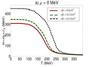
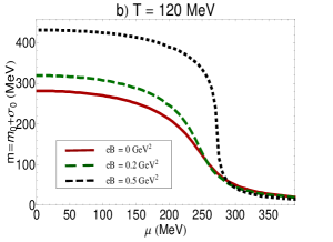
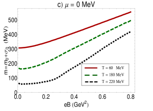
Figure 1: (a) and (b) The $T$ and $\mu$ dependence of the constituent quark mass $m=m_{0}+\sigma_{0}$ for fixed $eB=0,0.2,0.5$ GeV² and for fixed $\mu=0$ and $T=120$, respectively. Here, $m_{0}\simeq 5$ MeV is the bare quark mass and $\sigma_{0}$ is the chiral condensate. (c) The $eB$ dependence of $m$ is demonstrated for fixed $\mu=0$ and various $T=60,180$ and $220$ MeV.

Using the thermodynamic potential from (III.14), we will determine, in what follows, the chiral condensate and the complete phase portrait of the two-flavor NJL model at finite $T,\mu$ and $eB$. The notations and mathematical method used in this paragraph are similar to what was previously used in fayazbakhsh2010 . To determine the chiral condensate, we have to solve the gap equation numerically

$$\frac{\partial\Omega_{\mbox{\tiny{eff}}}(\bar{m};T,\mu,eB)}{\partial\bar{m}}\bigg{|}_{\bar{m}=m}=0.$$ (V.1)

Here, $\bar{m}=m_{0}+\sigma$ and $m=m_{0}+\sigma_{0}$, as are introduced in Sec. III. Our specific choice of parameters is buballa2004

$$\Lambda=0.6643~{}\mbox{GeV},~{}G=4.668~{}\mbox{GeV}^{-2},m_{0}=5~{}\mbox{MeV},$$

where $\Lambda$ is the UV momentum cutoff and $G$ is the NJL (chiral) coupling constant. To perform the momentum integration over ${\mathbf{p}}$ and $p_{3}$, we have introduced, as in fayazbakhsh2010 , smooth cutoff functions

$$f_{\Lambda} = \frac{1}{1+\exp\left(\frac{|{\mathbf{p}}|-\Lambda}{A}\right)},$$

$$f_{\Lambda,B}^{p} = \frac{1}{1+\exp\left(\frac{\sqrt{p_{3}^{2}+2|qeB|p}-\Lambda}{A}\right)},$$ (V.3)

corresponding to integrals with vanishing and non-vanishing magnetic fields, respectively. In $f_{\Lambda,B}^{p}$, $p$ labels the Landau levels. Moreover, $A$ is a free parameter, which determines the sharpness of the cutoff scheme. It is chosen to be $A=0.05\Lambda$, with $\Lambda$ given in (V.1). Using the above smooth cutoff procedure, the above choice of parameters leads for vanishing magnetic field and at $T=\mu=0$ to the constituent mass $m\simeq 308$ MeV. Let us notice that the solutions of (V.1) are in general “local” minima of the theory. Keeping $\sigma_{0}\neq 0$ and looking for “global” minima of the system described by $\Omega_{\mbox{\tiny{eff}}}(m;T,\mu,eB)$ from (III.14), it turns out that only in the regime $\mu\in[0,350]$ MeV, $T\in[0,390]$ MeV and $\tilde{e}B\in[0,0.8]$ GeV², the global minima of $\Omega_{\mbox{\tiny{eff}}}$ are described by nonzero $\sigma_{0}$. In these regimes, the chiral symmetry is spontaneously broken by non-vanishing $\sigma_{0}$. All our numerical computations in the present section are therefore limited to these regimes. Note that because of non-vanishing quark mass $m_{0}$, the transition from the chiral symmetry broken phase to the normal phase is a smooth crossover (see the descriptions below).

In Fig. 1, the $T,\mu$ and $eB$ dependence of $m$ are presented. In Fig. 1(a), the $T$-dependence of $m$ is demonstrated for fixed $\mu=0$ and $eB=0,0.2,0.5$ GeV². Although the transition from the chiral symmetry broken phase, with $m\neq 0$ to the normal phase, with $m\simeq m_{0}\approx 0$, is a smooth crossover, but as it turns out, for stronger magnetic fields the transition to the normal phase occurs for larger values of $T$, whereas for $eB=0$, this transition temperature into the crossover region is smaller. Moreover, at $T\in[0,100]$ MeV, where $m$ is almost constant, the value of $m$ increases with increasing $eB$. All these effects are related with the phenomena of magnetic catalysis klimenko1992 ; miransky1995 , according to which, magnetic fields enhance the production of $\sigma_{0}\sim\langle\bar{\psi}\psi\rangle$ condensate, even for very small coupling between the fermions, and therefore catalyze the dynamical chiral symmetry breaking. Similar effects occur also in Fig. 1(b), where $m$ is plotted as a function of $\mu$, at fixed $T=120$ MeV and for various $eB=0,0.2,0.5$ GeV². At $\mu=0$, for instance, the value of $m$ increases with increasing $eB$. In Fig. 1(c), the $eB$-dependence of $m$ is demonstrated for fixed $\mu=0$ and $T=60,180$ and $220$ MeV. As it turns out, for fixed value of $eB$, $m$ decreases with increasing $T$, and as it turns out, this “melting” effect persists in the whole range of $eB\in[0,0.8]$ GeV², although it is partly compensated by the magnetic field in the regime $eB>0.6$ GeV². Let us notice that, according to our results in fayazbakhsh2010-1 ; fayazbakhsh2010 , for a certain threshold magnetic field $eB_{t}\simeq 0.45$ GeV², the magnetic field is strong enough and forces the dynamics of the system to be mainly described by the LLL. In this regime, $m$ increases linearly with increasing $eB$ [see Fig. 1(c)]. Later, in rebhan2011 , the threshold magnetic field is estimated to be in the order of $B\simeq 10^{19}$ Gauß. In the present paper, however, the threshold magnetic field turns out to be $eB_{t}\geq 0.7$ GeV² [or equivalently $B\simeq 1.2\times 10^{20}$ Gauß]. The $T$ and $eB$ dependence of $m$ at fixed chemical potential $\mu$ and various $eB$ and $T$ are discussed recently in condensate-lattice using lattice gauge theory methods in the presence of constant (electro)magnetic fields. Our original results from fayazbakhsh2010 as well as the results presented in Figs. 1(a) and 1(c) are consistent with the results arising from lattice simulations condensate-lattice .

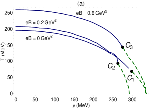
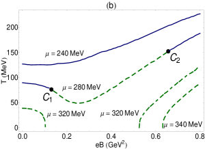
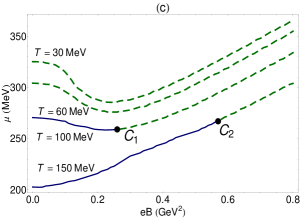
Figure 2: Complete phase portrait of a two-flavor magnetized NJL model at finite $T$, $\mu$ and $eB$ in the chiral limit of vanishing quark mass $m_{0}$. Blue solid (green dashed) lines denote the second (first) phase order phase transition between the chiral symmetry broken and normal phases. Two branches of the first order critical line for $\mu=320$ MeV are denoted by green double-dashed lines.

According to our results in fayazbakhsh2010 , in the chiral limit $m_{0}\to 0$ and for vanishing magnetic field, at high temperature and small chemical potential, the transition from the chiral symmetry broken to the normal phase is of second order. In contrast, at low temperatures and higher densities, the second order phase transition goes over to a first order one. In the presence of a uniform magnetic field, this picture remains essentially the same. The only difference is that for $\mu=0$, the transition temperature increases with increasing $eB$. Moreover, for $eB\neq 0$, the second order phase transition occurs at higher temperatures and lower densities comparing to the case of vanishing magnetic fields. These two effects of the uniform magnetic field on the $T-\mu$ phase diagram of a two-flavor NJL model in the chiral limit are demonstrated in Fig. 2(a). Both effects are manifestations of the phenomenon of magnetic catalysis in the presence of constant magnetic fields klimenko1992 ; miransky1995 . In all the plots of Fig. 2, the green dashed (blue solid) lines denote first (second) order phase transitions. To determine the first and second order phase transitions, the method described in sato1997 ; inagaki2003 ; fayazbakhsh2010 ; fayazbakhsh2010-1 is used. The first order critical lines between the chiral symmetry breaking and the normal phase is determined by solving

$$\frac{\partial\Omega_{\mbox{\tiny{eff}}}(\bar{m};T,\mu,eB)}{\partial\bar{m}}\bigg{|}_{m}=0,$$

$$\Omega_{\mbox{\tiny{eff}}}(m\neq 0;T,\mu,eB)=\Omega_{\mbox{\tiny{eff}}}(m=0;T,\mu,eB),$$ (V.4)

simultaneously. The second order critical line between these two phases is determined using

$$\lim_{m^{2}\rightarrow 0}\frac{\partial\Omega_{\mbox{\tiny{eff}}}(m;T,\mu,eB)}{\partial m^{2}}=0.$$ (V.5)

To make sure that after the second order phase transition the global minima of the effective potential are shifted to $m=0$ in (V.5), and in order to avoid instabilities, an analysis similar to berges1998 is also performed.

In Fig. 2(b), the $T-eB$ phase diagram of our model is plotted for various $\mu=240,280,320,340$ MeV. Let us notice that for $\mu=320$ MeV [dashed-dotted lines in Fig. 2(b)], the first order critical line has two branches – the first one for $eB<0.1$ GeV² and the second one for $eB>0.5$ GeV², at relatively low temperature. In the intermediate region $0.1<eB<0.5$ GeV², the chiral symmetry breaking phase is disfavored. In fayazbakhsh2010 , we have studied the $T-eB$ phase diagram of a two-flavor NJL model including meson and diquark condensates. We have shown that in the above mentioned intermediate regime $0.1<eB<0.5$ GeV² at low temperature and for $\mu=320$ MeV, the two-flavor color superconducting (2SC) phase is favored. For $\mu>320$ MeV, the first branch appearing for $\mu=320$ MeV and $eB<0.1$ GeV² disappears, and the whole region of $eB<0.6$ GeV² is favored by either the normal phase, when no diquarks exist in the model, or by the 2SC superconducting phase, when the model includes both meson and diquark condensates (see Fig. 14 of fayazbakhsh2010 ).

In Fig. 2(c), the $\mu-eB$ phase diagram of our two-flavor NJL model including chiral condensates $(\sigma,\vec{\pi})$ is plotted for various $T=30,60,100,150$ MeV. At very low temperature, $T<100$ MeV, the transition between the chiral symmetry breaking and normal phase is of first order (green dashed lines). Whereas at these temperatures and for $eB<0.1$ GeV², the critical $\mu$ is almost constant, it decreases by increasing the strength of the magnetic field in the regime $0.1<eB<0.4$ GeV². This effect, which is for the first time observed in fayazbakhsh2010-1 ; fayazbakhsh2010 , and later also in rebhan2011 , is called the “inverse magnetic catalysis”, according to which at low temperature, the addition of the magnetic field decreases the critical chemical potential for chiral symmetry restoration fayazbakhsh2010 ; rebhan2011 . However, by increasing the magnetic field up to $eB>0.5$ GeV², i.e. by entering the regime of LLL dominance, this effect is disfavored, so that $\mu_{c}$ again increases with increasing the strength of the magnetic field. Let us also note that similar phenomenon of inverse magnetic catalysis appears also in Fig. 2(b), where for fixed $\mu=280$ MeV, the first order critical line $T_{c}$ (green dashed line between $C_{1}$ and $C_{2}$) decreases with increasing $eB$ from $0.1<eB<0.3$ GeV² and continues to grow up with increasing the strength of the magnetic field up to regime of LLL dominance, i.e $eB>0.5$ GeV². The inverse magnetic catalysis effect may be related to the well-known van-alphen–de Haas oscillations, which occur whenever Landau levels pass the quark Fermi level alfven . Similar effects are also observed in inagaki2003 ; fayazbakhsh2010 ; fayazbakhsh2010-1 . At higher temperature $T>100$ MeV and for $eB$ smaller than a certain critical $eB_{c}$, there is a second order phase transition between the chiral symmetry broken and normal phases (see the blue solid lines in Fig. 2(c) for $T=100,150$ MeV, that replace the green dashed lines for $T<100$ MeV). The critical magnetic field $eB_{c}$, for which the second order phase ends and goes over into a first order phase transition is larger for higher temperature [compare $eB_{c}$ for two critical points (black bullets) $C_{1}$ and $C_{2}$ in Fig. 2(c)]. This demonstrates the destructive effect of the temperature, which is partly compensated in the regime of strong magnetic fields, $eB>0.7$ GeV². More details on the interplay between three parameters $T,\mu$ and $eB$ on the formation of chiral condensates $\sigma_{0}$ in the chiral limit $m_{0}\to 0$ are discussed in fayazbakhsh2010 .

V.2 $(M_{\sigma}^{2},M_{\pi^{0}}^{2})$ and $({\cal{G}}^{\mu\nu},{\cal{F}}^{\mu\nu})$ at $(T\neq 0,\mu=0,eB\neq 0)$

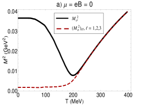
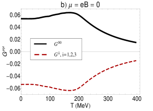
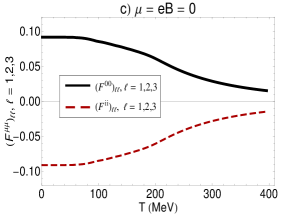
Figure 3: The $T$-dependence of $(M_{\sigma}^{2},(M_{\vec{\pi}}^{2})_{\ell\ell})$ as well as $({\cal{G}}^{00},{\cal{G}}^{ii})$, and $(({\cal{F}}^{00})_{\ell\ell},({\cal{F}}^{ii})_{\ell\ell})$ with $\ell,i=1,2,3$ for vanishing magnetic field $eB$ and at $\mu=0$.

As we have described in the first part of this section, the results presented in (IV.30) and (IV.38) for $M_{\sigma}^{2}$ and $M_{\pi^{0}}^{2}$, and in (IV.2.1) and (IV.59) for ${\cal{G}}^{\mu\nu}$ as well as in (IV.2.2) and (IV.64) for ${\cal{F}}^{\mu\nu}$ are given up to an integration over $p_{3}$-momentum and a summation over Landau levels $p$. We have performed the $p_{3}$-integration for the set of parameters $(\Lambda,G,m_{0})$ from (V.1) and the smooth cutoff function (V.1) numerically, and will present the results in what follows. In particular, we will present the $T$-dependence of $(M_{\sigma}^{2},M_{\pi^{0}}^{2})$ and $({\cal{G}}^{\mu\nu},{\cal{F}}^{\mu\nu})$ for fixed $\mu=0$ and various $eB=0,0.03,0.2,0.3$ GeV².

Let us start by giving the numerical values of $(M_{\sigma}^{2},M_{\vec{\pi}}^{2})$ and $({\cal{G}}^{\mu\nu},{\cal{F}}^{\mu\nu})$ at $T=\mu=eB=0$. According to their definitions in (IV.4)-(LABEL:ND7b), where, for $eB=0$, $S_{Q}$ is to be replaced by the ordinary fermion propagator $S(z,0)=\int\frac{d^{4}p}{(2\pi)^{4}}\frac{ie^{-ip\cdot z}}{\gamma\cdot p-m}$ at zero $(T,\mu)$, we have the following identities and numerical values

$$M_{\sigma}^{2} = 3.656\times 10^{-2}\mbox{GeV}^{2},$$

$$M_{\pi_{\ell}}^{2} = 1.734\times 10^{-3}\mbox{GeV}^{2},~{}~{}~{}\forall\ell=1,2,3,$$ (V.6)

as well as

$${\cal{G}}^{00} = -{\cal{G}}^{ii}~{}~{}~{}~{}~{}\qquad\forall i=1,2,3,$$

$$({\cal{F}}^{00})_{\ell\ell} = -({\cal{F}}^{ii})_{\ell\ell}\qquad\forall i=1,2,3,$$ (V.7)

where

$${\cal{G}}^{00} = 5.381\times 10^{-2},$$

$$({\cal{F}}^{00})_{\ell\ell} = 9.143\times 10^{-2},\qquad\forall\ell=1,2,3.$$ (V.8)

Moreover, we have $({\cal{F}}^{ii})_{11}=({\cal{F}}^{ii})_{22}=({\cal{F}}^{ii})_{33}$ for all $i=0,\cdots,3$.

At finite temperature and vanishing $\mu$ and $eB$, although the above relations (V.2) and (V.2) between different components of $M_{\vec{\pi}}^{2}$ as well as ${\cal{G}}^{\mu\nu}$ and ${\cal{F}}^{\mu\nu}$ are still valid, i.e. we have

$$(M_{\vec{\pi}}^{2})_{11}=(M_{\vec{\pi}}^{2})_{22}=(M_{\vec{\pi}}^{2})_{33},$$ (V.9)

as well as

$${\cal{G}}^{00} = -{\cal{G}}^{11}=-{\cal{G}}^{22}=-{\cal{G}}^{33},$$

$$({\cal{F}}^{00})_{\ell\ell} = -({\cal{F}}^{ii})_{\ell\ell},\qquad\forall\ell,i=1,2,3,$$ (V.10)

but their values become temperature dependent. In Fig. 3, the $T$-dependence of $(M_{\sigma}^{2},(M_{\vec{\pi}}^{2})_{\ell\ell})$ as well as $({\cal{G}}^{00},{\cal{G}}^{ii})$, and $(({\cal{F}}^{00})_{\ell\ell},({\cal{F}}^{ii})_{\ell\ell})$ with $\ell,i=1,2,3$ are plotted for vanishing $eB$ and $\mu$. As it is demonstrated in Fig. 3(a), $M^{2}_{\sigma}$ and $(M_{\vec{\pi}}^{2})_{\ell\ell}$ are degenerate at $T>220$ MeV. This is because the difference between these two functions are in terms proportional to the constituent quark mass $m=m_{0}+\sigma_{0}$, that, according to Fig. 1(a) almost vanishes in the crossover region $T>220$ MeV. Later, we will show that the degeneracy of $M^{2}_{\sigma}$ and $(M_{\vec{\pi}}^{2})_{\ell\ell}$ for $T>220$ MeV leads to the expected degeneracy of $\sigma$ and $\pi^{0}$ meson masses $(m_{\sigma},m_{\pi^{0}})$ for vanishing $eB$ and $\mu$ in the crossover region $T>220$ MeV buballa2012 .

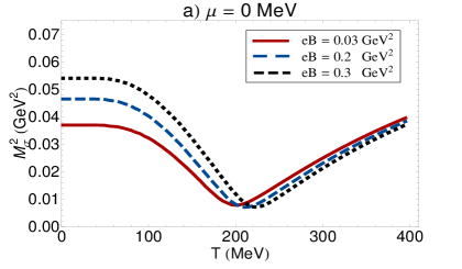
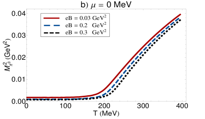
Figure 4: The coefficient $M_{\sigma}^{2}$ (panel a) and $M_{\pi^{0}}^{2}$ (panel b), are plotted as functions of $T\in[0,400]$ MeV at $\mu=0$ and for $eB=0.03,0.2,0.3$ GeV² (red solid, blue dashed and black dotted lines, respectively) .

Let us finally consider the case of $(T,eB\neq 0,\mu=0)$. As it turns out, the degeneracy in $(M_{\vec{\pi}}^{2})_{\ell\ell}$ as well as ${\cal{G}}^{ii}$ and $({\cal{F}}^{ii})_{\ell\ell}$, with $\ell,i=1,2,3$ at $(T,eB\neq 0,\mu=0)$ breaks down by finite magnetic fields. In other words, for $(T,eB\neq 0,\mu=0)$, in contrast to (V.9), we have

$$(M_{\vec{\pi}}^{2})_{11}=(M_{\vec{\pi}}^{2})_{22}\neq(M_{\vec{\pi}}^{2})_{33}.$$ (V.11)

Moreover, in contrast to (V.2)

$${\cal{G}}^{00}=-{\cal{G}}^{33}\neq{\cal{G}}^{11}={\cal{G}}^{22}.$$ (V.12)

Similarly, in contrast to (V.2), although $({\cal{F}}^{\mu\mu})_{11}=({\cal{F}}^{\mu\mu})_{22}\neq({\cal{F}}^{\mu\mu})_{33}$, for all $\mu=0,\cdots,3$, but

$$({\cal{F}}^{00})_{\ell\ell}=-({\cal{F}}^{33})_{\ell\ell}\neq({\cal{F}}^{11})_{\ell\ell}=({\cal{F}}^{22})_{\ell\ell},$$ (V.13)

$\forall~{}\ell=1,2,3$. In Fig. 4, the $T$-dependence of $M_{\sigma}^{2}$ (panel a) and $M_{\pi^{0}}^{2}$ [or equivalently, $(M_{\vec{\pi}}^{2})_{33}$] (panel b) are demonstrated at $\mu=0$ and for non-vanishing $eB=0.03,0.2,0.3$ GeV². The exact $(T,\mu,eB)$ dependence of $(M_{\vec{\pi}}^{2})_{11}=(M_{\vec{\pi}}^{2})_{22}$ will be used in sadooghi2012-3 , to determine the $(T,\mu,eB)$-dependence of charged pion masses.

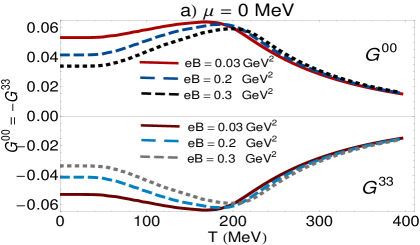
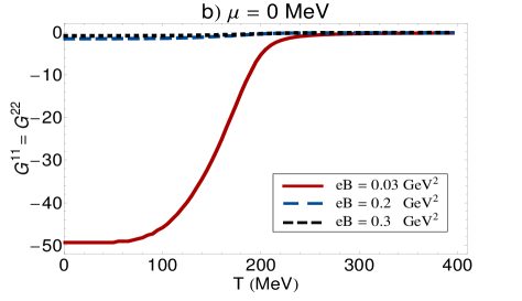
Figure 5: The coefficients ${\cal{G}}^{00}=-{\cal{G}}^{33}$ (panel a), ${\cal{G}}^{11}={\cal{G}}^{22}$ (panel b) are plotted as functions of $T\in[0,400]$ MeV for $\mu=0$ and $eB=0.03,0.2,0.3$ GeV².

In Fig. 5, the $T$-dependence of ${\cal{G}}^{00}$ and ${\cal{G}}^{33}$ (${\cal{G}}^{00}=-{\cal{G}}^{33}$) (panel a) as well as ${\cal{G}}^{11}={\cal{G}}^{22}$ (panel b) are plotted for $\mu=0$ and $eB=0.03,0.2,0.3$ GeV². Whereas ${\cal{G}}^{00}$ is positive, ${\cal{G}}^{11}={\cal{G}}^{22}$ and ${\cal{G}}^{33}$ are negative. Later, we will use the matrix elements of $M_{\sigma}^{2}$ from Fig. 4 and the coefficients ${\cal{G}}^{\mu\mu},\mu=0,\cdots,3$ from Fig. 5, to determine the $T$-dependence of $m_{\sigma}$ at $\mu=0$ and for various $eB\neq 0$.

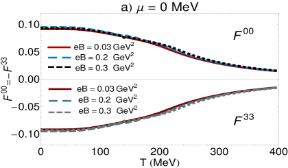
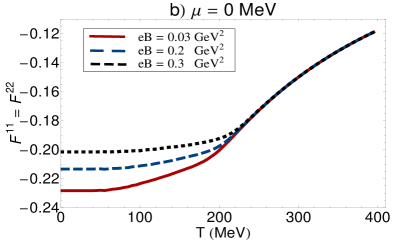
Figure 6: The diagonal elements of ${\cal{F}}^{\mu\mu},\mu=0,\cdots,3$ matrices are plotted as functions of $T\in[0,400]$ MeV at vanishing chemical potential ($\mu=0$) and for $eB=0.03,0.2,0.3$ GeV². The identities from (V.13) for $\ell=3$, ${\cal{F}}^{11}={\cal{F}}^{22}$ and ${\cal{F}}^{00}=-{\cal{F}}^{33}$, are explicitly demonstrated in these plots.

In Fig. 6, the $T$-dependence of ${\cal{F}}^{\mu\mu},\mu=0,\cdots,3$ [or equivalently, $({\cal{F}}^{\mu\mu})_{33}$] matrices are plotted for vanishing chemical potential and $eB=0.03,0.2,0.3$ GeV². In the subsequent section, we will in particular use $M_{\pi^{0}}^{2}$, ${\cal{F}}^{00}$ and ${\cal{F}}^{33}$ to determine the $T$-dependence of $\pi^{0}$ pole and screening masses as well as the direction-dependent refraction indices of neutral pion in the longitudinal and transverse directions with respect to the direction of the external magnetic field.

V.3 Masses and directional refraction indices of neutral mesons

In this section, we will use the results obtained in Sec. V.2 to determine the $T$-dependence of pole and screening masses as well as the direction-dependent refraction indices of neutral mesons, $\sigma$ and $\pi^{0}$, in a hot and dense magnetized quark matter. In what follows, we will first define these quantities according to the descriptions presented in Sec. II and the corresponding energy dispersion relations for neutral and charged mesons $\sigma$ and $\pi_{\ell},\ell=1,2,3$ mesons [see also (II.15) and (II)],

$$E_{\sigma}^{2} = \frac{1}{{\cal{G}}^{00}}\left({\cal{G}}^{11}p_{1}^{2}+{\cal{G}}^{22}p_{2}^{2}+{\cal{G}}^{33}p_{3}^{2}+M_{\sigma}^{2}\right),$$

$$E_{\pi_{\ell}}^{2}\hskip 1.42271pt=$$

$$\frac{1}{({\cal{F}}^{00})_{\ell\ell}}\big{[}({\cal{F}}^{11})_{\ell\ell}p_{1}^{2}+({\cal{F}}^{22})_{\ell\ell}p_{2}^{2}+({\cal{F}}^{33})_{\ell\ell}p_{3}^{2}+M_{\pi_{\ell}}^{2}\big{]}.$$

The pole and screening masses of $\sigma$-mesons, $m_{\sigma}$ and $m_{\sigma}^{(i)},i=1,2,3$, are then defined by

$$m_{\sigma}=\bigg{[}\frac{\mbox{Re}~{}M_{\sigma}^{2}}{\mbox{Re}~{}{\cal{G}}^{00}}\bigg{]}^{1/2},~{}~{}\mbox{as well as}~{}~{}m_{\sigma}^{(i)}=\frac{m_{\sigma}}{u_{\sigma}^{(i)}},$$ (V.15)

where, $u_{\sigma}^{(i)}$, is the directional refraction index of $\sigma$-mesons in the $i$-th direction,

$$u_{\sigma}^{(i)}=\bigg{|}\frac{\mbox{Re}~{}{\cal{G}}^{ii}}{\mbox{Re}~{}{\cal{G}}^{00}}\bigg{|}^{1/2},\qquad i=1,2,3.$$ (V.16)

The $(T,\mu,eB)$-dependence of $m_{\sigma},m_{\sigma}^{(i)}$ and $u_{\sigma}^{(i)}$ are given by plugging $M_{\sigma}^{2}$ and ${\cal{G}}^{\mu\mu},\mu=0,\cdots,3$ from (IV.30), (IV.2.1) and (IV.59) in the above relations. As concerns the pions, we choose the basis $(\pi^{\pm},\pi^{0})$ instead of the real basis $\vec{\pi}=(\pi_{1},\pi_{2},\pi_{3})$. Here, $\pi^{\pm}\equiv(\pi_{1}\pm i\pi_{2})/\sqrt{2}$ and $\pi^{0}\equiv\pi_{3}$. Using this new imaginary basis, the energy dispersion relations $E_{\pi_{\ell}}$ from (V.3) for $(\pi^{\pm},\pi^{0})$ turn out to be

$$E_{\pi^{\pm}}^{2}\equiv\frac{eB(2\ell+1)}{[({\cal{F}}^{00})_{11}\mp i({\cal{F}}^{00})_{12}]}$$

$$+\frac{[({\cal{F}}^{33})_{11}\mp i({\cal{F}}^{33})_{12}]}{[({\cal{F}}^{00})_{11}\mp i({\cal{F}}^{00})_{12}]}p_{3}^{2}+\frac{[(M_{\vec{\pi}}^{2})_{11}\mp i(M_{\vec{\pi}}^{2})_{12}]}{[({\cal{F}}^{00})_{11}\mp i({\cal{F}}^{00})_{12}]},$$

$$E_{\pi^{0}}^{2}\equiv\frac{({\cal{F}}^{11})_{33}}{({\cal{F}}^{00})_{33}}~{}p_{1}^{2}$$ (V.17)

$$+\frac{({\cal{F}}^{22})_{33}}{({\cal{F}}^{00})_{33}}~{}p_{2}^{2}+\frac{({\cal{F}}^{33})_{33}}{({\cal{F}}^{00})_{33}}~{}p_{3}^{2}+\frac{(M_{\vec{\pi}}^{2})_{33}}{({\cal{F}}^{00})_{33}}.$$

Note that since $\pi^{\pm}$ are charged pseudoscalar particles, their energy dispersion relations in the presence of constant magnetic fields have discrete contributions. According to our results in jafarisalim2006 , the energy levels are labeled by $\ell$, in the form given in the first term in (V.3). The above dispersion relations for charged pions are comparable with the dispersion relations presented recently in anderson2012-2 (see Eq. (2.10) in anderson2012-2 ). According to the formalism presented originally in miransky1995 and generalized to a multi-flavor system in the present paper, in contrast to the relations presented in anderson2012-2 for charged pions, the nontrivial form factors $({\cal{F}}^{\mu\mu})_{\ell m}$, $\forall~{}\ell,m\neq 3$ in (V.3), consider the effect of external magnetic fields on charged quarks produced at the early stage of the heavy-ion collisions. Moreover, in the formalism presented in anderson2012-2 , in contrast to the dispersion relations presented in (V.3), the energy dispersion relation of neutral pion is unaffected by the external magnetic field. Using (V.3), and in analogy to (V.15), the pions pole masses are defined by

$$m_{\pi^{\pm}} = \bigg{[}\frac{\mbox{Re}~{}[(M_{\vec{\pi}}^{2})_{11}\mp i(M_{\vec{\pi}}^{2})_{12}]}{\mbox{Re}~{}[({\cal{F}}^{00})_{11}\mp i({\cal{F}}^{00})_{12}]}\bigg{]}^{1/2},$$

$$m_{\pi^{0}} = \bigg{[}\frac{\mbox{Re}~{}(M_{\pi}^{2})_{33}}{\mbox{Re}~{}({\cal{F}}^{00})_{33}}\bigg{]}^{1/2}.$$ (V.18)

In particular, the screening mass and the refraction index of neutral pions in the $i$-th direction are given by

$$m_{\pi^{0}}^{(i)}=\frac{m_{\pi^{0}}}{u_{\pi^{0}}^{(i)}},~{}~{}~{}\mbox{and}~{}~{}~{}u_{\pi^{0}}^{(i)}=\bigg{|}\frac{\mbox{Re}~{}({\cal{F}}^{ii})_{33}}{\mbox{Re}~{}({\cal{F}}^{00})_{33}}\bigg{|}^{1/2},$$ (V.19)

respectively. In this paper, we will focus on the $T$-dependence of the mass and refraction index of neutral pions at fixed $\mu$ and finite $eB$. The study of the effect of constant magnetic fields on charged pion masses and refraction indices will be postponed to a future publication sadooghi2012-3 .

Let us start with the case $T=\mu=eB=0$. Using the numerical results from (V.2) and (V.2), in this case, the $\sigma$-meson mass and refraction index are given by

$$m_{\sigma}\simeq 824.3~{}\mbox{MeV},\qquad\mbox{and}\qquad u_{\sigma}^{(i)}=1,$$ (V.20)

and therefore

$$m_{\sigma}^{(i)}=m_{\sigma},~{}\forall i=1,2,3.$$ (V.21)

Similarly, the $\vec{\pi}$-meson mass and refraction index at $T=\mu=eB=0$ read

$$m_{\pi_{\ell}}\simeq 137.7~{}\mbox{MeV},\qquad\mbox{and}\qquad u_{\pi_{\ell}}^{(i)}=1,$$ (V.22)

$\forall~{}\ell,i=1,2,3$, and therefore

$$m_{\pi_{\ell}}^{(i)}=m_{\pi_{\ell}},~{}\forall\ell,i=1,2,3.$$ (V.23)

At $(T\neq 0,\mu=eB=0)$, $m_{\sigma}$ is given by (V.15). Similarly, according to (V.3), the pion masses $m_{\vec{\pi}}$ are defined by

$$m_{\pi_{\ell}}=\bigg{[}\frac{\mbox{Re}~{}(M_{\vec{\pi}}^{2})_{\ell\ell}}{\mbox{Re}~{}({\cal{F}}^{00})_{\ell\ell}}\bigg{]}^{1/2},\qquad\forall\ell=1,2,3.$$ (V.24)

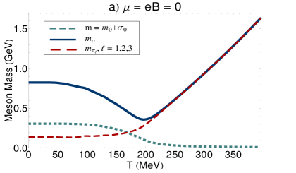
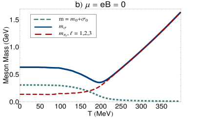
Figure 7: (a) The $T$-dependence of $\sigma$ and $\vec{\pi}$ mesons masses is demonstrated at $\mu=0$ and for vanishing magnetic field (solid line for $m_{\sigma}$ and dashed line for $m_{\vec{\pi}}$). Comparing these curves with the $T$-dependence of the constituent quark mass $m=m_{0}+\sigma_{0}$ (dotted line), shows that a mass degeneracy between $m_{\sigma}$ and $m_{\vec{\pi}}$ occurs in the crossover region at $T>220$ MeV. (b) The $T$-dependence of the pole masses of neutral mesons is plotted for the case when $F_{2}^{\mu\nu}$ in (II) vanishes. The numerical results for $m_{\sigma}$ and $m_{\vec{\pi}}$ are in good agreement with the results recently presented in buballa2012 .

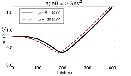
Figure 8: The $T$-dependence of $m_{\sigma}$ (panel a) and $m_{\vec{\pi}}$ (panel b) is plotted for $eB=0$ and at $\mu=0,120$ MeV. As in the case of $\mu=0$, at $\mu=120$ MeV, the neutral meson masses are still degenerate in the crossover region $T>220$ MeV.

Because of the identity (V.9), which is still valid at $(T\neq 0,\mu=eB=0)$, the masses of $\vec{\pi}=(\pi_{1},\pi_{2},\pi_{3})$ are degenerate, as in $T=0$ case [see (V.22)]. In Fig. 7(a), the $T$-dependence of $m_{\sigma}$ and $m_{\vec{\pi}}$ is plotted for $\mu=eB=0$ (black solid line for $m_{\sigma}$ and red dashed line for $m_{\vec{\pi}}$). Here, the $T$-dependence of the coefficients ${\cal{G}}^{\mu\mu}$ and ${\cal{F}}^{\mu\mu}$ from Fig. 3 is used. We have also plotted the $T$-dependence of the constituent mass $m=m_{0}+\sigma_{0}$ in Fig. 7(a) (dotted line). Comparing these curves, it turns out that, as expected, the mass degeneracy of $\sigma$ and $\vec{\pi}$ meson masses occurs in the crossover region $T>220$ MeV. To compare the result presented in Fig. 7(a), with the recent results for $m_{\vec{\pi}}$ and $m_{\sigma}$, presented e.g. in buballa2012 , we have set $F_{2}^{\mu\nu}=0$ in (II), and determined the pole masses of neutral mesons and the chiral condensate using the same method as presented in this paper. The numerical results for neutral meson masses and chiral condensate for $T\neq 0$, $\mu=eB=0$ and vanishing $F_{2}^{\mu\nu}$ are plotted in Fig. 7(b). As it turns out, only $m_{\sigma}$ changes relative to the case where $F_{2}^{\mu\nu}\neq 0$ [see Fig. 7(b)]. The numerical results are in good agreement with the results presented in buballa2012 .

As concerns the screening mass and refraction index of $\vec{\pi}$ mesons at $(T\neq 0,\mu=eB=0)$, we use the results of Fig. 3, and in analogy to the definitions (V.15) and (V.16) define the screening mass and refraction index of $\vec{\pi}$ mesons by

$$m_{\pi_{\ell}}^{(i)} = \frac{m_{\pi_{\ell}}}{u_{\pi_{\ell}}^{(i)}},\qquad\mbox{where}$$

$$u_{\pi_{\ell}}^{(i)} = \bigg{|}\frac{\mbox{Re}~{}({\cal{F}}^{ii})_{\ell\ell}}{\mbox{Re}~{}({\cal{F}}^{00})_{\ell\ell}}\bigg{|}^{1/2},~{}~{}\forall\ell,i=1,2,3.$$ (V.25)

Using the definitions (V.16) and (V.3), and the numerical results of ${\cal{G}}^{00}$ as well as $({\cal{F}}^{00})_{\ell\ell}$ from Fig. 3 at $(T\neq 0,\mu=eB=0)$, the $T$-dependence of the screening mass and refraction index of $(\sigma,\vec{\pi})$ mesons can be determined for all directions $i=1,2,3$. As it turns out, as in $T=0$ case, we have

$$\begin{array}[]{rclcrcl}u_{\sigma}^{(i)}&=&1,&&\forall i&=&1,2,3,\\ u_{\pi_{\ell}}^{(i)}&=&1,&&\forall\ell,i&=&1,2,3,\end{array}$$ (V.28)

and therefore

$$\begin{array}[]{rclcrcl}m_{\sigma}^{(i)}&=&m_{\sigma},&&\forall i&=&1,2,3,\\ m_{\pi_{\ell}}^{(i)}&=&m_{\pi_{\ell}},&&\forall\ell,i&=&1,2,3,\end{array}$$ (V.31)

for the whole interval $T\in[0,400]$. These results are compatible with the identities (V.2). The fact that $u_{\pi_{\ell}}=1$ seems to be in contradiction with the results from son2000 ; ayala2002 , where it is shown that at finite temperature because of different pion decay constants in the spatial and temporal directions, $f_{s}$ and $f_{t}$, at finite temperature, the refraction index $u=\frac{f_{s}}{f_{t}}$ appearing in the energy dispersion relation $\omega^{2}=u^{2}(\mathbf{p}^{2}+m^{2})$ is smaller than one. Note, however, that in son2000 ; ayala2002 , the pions are self-interacting and $f_{s}$ and $f_{t}$ receive $T$-dependent contributions from one-loop pion-self energy diagram, that includes a $(\vec{\pi}^{2})^{2}$ vertex. In contrast, the pions considered in the present paper are free.

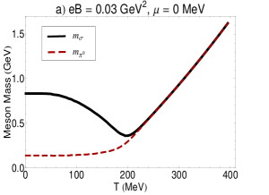
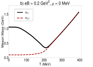
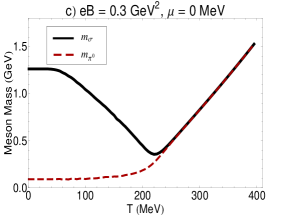
Figure 9: The $T$-dependence of $m_{\sigma}$ and $m_{\pi^{0}}$ is plotted for $eB=0.03,0.2,0.3$ GeV² and at $\mu=0$ MeV.

Let us also notice that the above results are still valid at non-vanishing $\mu$ and for vanishing $eB$. In Fig. 8, we have compared $m_{\sigma}$ and $m_{\pi_{\ell}},\ell=1,2,3$ at $\mu=0$ with their values at $\mu=120$ MeV for vanishing $eB$. Small deviations from their value at $\mu=0$ appears for $m_{\sigma}$ (panel a). For $m_{\pi_{\ell}},\ell=1,2,3$ (panel b) the difference between $m_{\pi_{\ell}}$ at $\mu=0$ and $\mu=120$ MeV becomes larger with increasing temperature. As it turns out, at non-vanishing chemical potential, the degeneracy of the pion masses $m_{\pi_{\ell}}$ is still valid for all $\ell=1,2,3$. Moreover, $m_{\sigma}$ and $m_{\vec{\pi}}$ are also degenerate in the crossover region $T>220$ MeV for $\mu=120$ MeV, as in the $\mu=0$ case.

At finite $T$ and for non-vanishing magnetic fields, the pion masses are not degenerate, i.e. we have $m_{\pi^{+}}\neq m_{\pi^{-}}\neq m_{\pi^{0}}$ [see (V.11) and (V.12) and the definitions of $m_{\pi^{\pm}}$ and $m_{\pi^{0}}$ from (V.3)]. In this paper, we will focus on the $T$-dependence of $m_{\sigma}$ and $m_{\pi^{0}}$. In Figs. 9(a)-9(c), the $T$-dependence of $(m_{\sigma},m_{\pi^{0}})$ masses are plotted for $eB=0.03,0.2,0.3$ GeV² and at $\mu=0$. The expected degeneracy of $m_{\sigma}$ and $m_{\pi^{0}}$ mesons in the crossover region can be observed in all the plots of Fig. 9. However, as it turns out, the overlap interval depends on $eB$ for fixed $\mu$. Denoting the minimum temperature for which the overlap interval starts with $T_{o}$, then for $eB=0.03$ GeV² we have $T_{o}\simeq 210$ MeV, whereas for $eB=0.2,0.3$ GeV², $T_{o}$ are given by $T_{o}\simeq 220$ MeV and $T_{o}\simeq 240$ MeV, respectively.

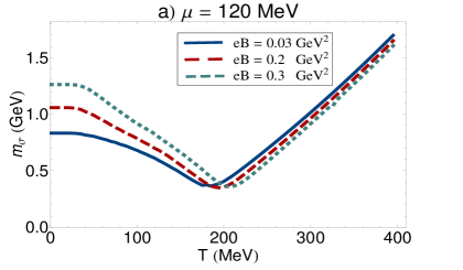
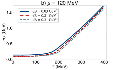
Figure 10: The $T$-dependence of $m_{\sigma}$ (panel a) and $m_{\pi^{0}}$ (panel b) is plotted for $eB=0.03,0.2,0.3$ GeV² at $\mu=120$ MeV.

In Fig. 10, we have compared the $T$-dependence of the masses of $\sigma$ and $\pi^{0}$ mesons for fixed $\mu=120$ MeV and various $eB=0.03,0.2,0.3$ GeV². As it turns out, at temperature below (above) the crossover region, the $\sigma$-meson masses increase (decrease) with increasing the magnetic field strength. This qualitative behavior of the $T$-dependence of $m_{\sigma}$ for various $eB\neq 0$ is comparable with the results presented in skokov2011 (see Fig. 3 in skokov2011 ). The difference arises from the fact that, in contrast to the present paper, the quantum fluctuations of $\sigma$-mesons is considered in skokov2011 . And, in contrast to the present paper, the contribution of $F_{2}^{\mu\nu}$ appearing in (II) is not considered in skokov2011 .

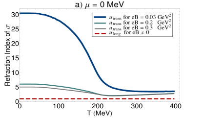
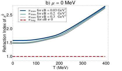
Figure 11: The $T$-dependence of the transverse and longitudinal refraction indices of $\sigma$ (panel a) and $\pi^{0}$ mesons (panel b) is plotted for various $eB$. The longitudinal refraction index of neutral mesons is equal to unity and independent of $T$ (red dashed lines). The transverse refraction index of neutral mesons decreases with increasing the strength of $eB$.

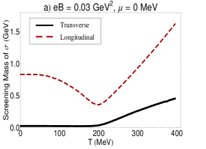
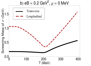
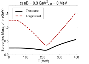
Figure 12: The $T$-dependence of the screening mass of $\sigma$ mesons, $m_{\sigma}^{(i)}$, from (V.15) in the transverse $(i=1,2)$ and longitudinal $(i=3)$ directions is plotted for various $eB$. As it turns out, the screening mass of the $\sigma$-meson in the longitudinal direction $m_{\sigma}^{(i)},i=3$ is the same as its pole mass $m_{\sigma}$ (see $m_{\sigma}$ in Fig. 9).

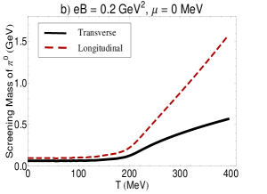
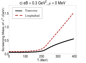
Figure 13: The $T$-dependence of the screening mass of $\pi^{0}$ mesons, $m_{\pi^{0}}^{(i)}$, from (V.19) in the transverse $(i=1,2)$ and longitudinal $(i=3)$ directions is plotted for various $eB$. As it turns out, the screening mass of the $\pi^{0}$-meson in the longitudinal direction $m_{\pi^{0}}^{(i)},i=3$ is the same as its pole mass $m_{\pi^{0}}$ (see $m_{\pi^{0}}$ in Fig. 9).

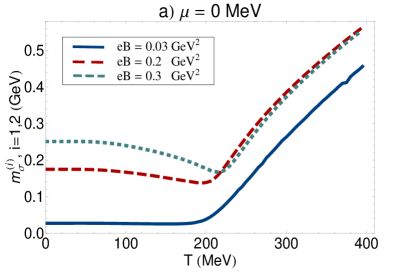
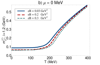
Figure 14: The $T$-dependence of the screening mass of $\sigma$ (panel a) and $\pi^{0}$ (panel b) mesons in the transverse direction is plotted for $eB=0.03,0.2,0.3$ GeV² at $\mu=0$ MeV.

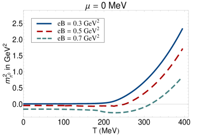
Figure 15: The $T$-dependence of the squared mass of neutral pion is plotted for $eB=0.3,0.5,0.7$ GeV².

Using the definitions of the directional refraction index of neutral mesons, $u_{\sigma}^{(i)}$ and $u_{\pi^{0}}^{(i)}$, from (V.16) and (V.19), as well as the $T$-dependence of ${\cal{G}}^{\mu\mu},\mu=0,\cdots,3$ and ${\cal{F}}^{\mu\mu},\mu=0,\cdots,3$ from Figs. 5 and 6, the $T$-dependence of the transverse ($i=1,2$) and longitudinal ($i=3$) refraction indices of $\sigma$ and ${\pi}^{0}$ mesons, are plotted in Fig. 11. From ${\cal{G}}^{00}=-{\cal{G}}^{33}$ as well as $({\cal{F}}^{00})_{33}=-({\cal{F}}^{33})_{33}$ in (V.12) as well as (V.13), the refraction index of neutral mesons in the longitudinal direction turn out to be equal to unity, independent of $T$ and $\mu$ (see the horizontal red dashed line in Fig. 11). In contrast, the relations ${\cal{G}}^{11}\neq{\cal{G}}^{00}$ as well as $({\cal{F}}^{11})_{33}\neq({\cal{F}}^{00})_{33}$ from (V.12) as well as (V.13), lead to $u_{\sigma}^{(i)}\neq 1$ as well as $u_{\pi^{0}}^{(i)}\neq 1$ for $i=1,2$. In Fig. 11, the $T$-dependence of the transverse and longitudinal refraction indices of free and neutral mesons are plotted for $eB=0.03,0.2,0.3$ GeV² and $\mu=0$ MeV. As it turns out, in the presence of constant magnetic fields, the transverse refraction indices of neutral mesons are always larger than unity. Moreover, the transverse refraction index of $\sigma$ ($\pi^{0}$) meson decreases (increases) with increasing temperature. Note that transverse refraction indices of neutral mesons decrease with increasing the strength of the background magnetic fields. It is interesting to add the effect of meson fluctuations to the above results and recalculate the $T$-dependence of longitudinal and transverse refraction indices of neutral mesons for non-vanishing $eB$ and $\mu$.

Using the definition of the screening masses $m_{\sigma}^{(i)}$ from (V.15) and $m_{\pi^{0}}^{(i)}$ from (V.19), we arrive at the $T$-dependence of the screening masses of neutral mesons at $\mu=0$ and for fixed $eB=0.03,0.2,0.3$ MeV. Since in the longitudinal direction ($i=3$), the directional refraction index of $\sigma$ and $\pi^{0}$ mesons is equal to unity, the screening masses of the neutral mesons in this direction are the same as their pole masses $m_{\sigma}$ and $m_{\pi^{0}}$. In Figs. 12 and 13, the $T$-dependence of the screening masses of $\sigma$ and $\pi^{0}$ mesons in the transverse ($i=1,2$) and longitudinal ($i=3$) directions with respect to the direction of the external magnetic field are demonstrated. As it turns out, the screening mass of $\sigma$ and $\pi^{0}$ mesons in the transverse directions are for all fixed $eB$ always smaller than the screening masses in the longitudinal direction. In Figs. 14(a) and (b), we have compared the screening masses of $\sigma$ and $\pi^{0}$ mesons in the transverse directions ($i=1,2$), respectively. Comparing with the plots of Figs. 10(a) and (b), it turns out, that, in contrast to $m_{\pi^{0}}^{(i)},i=1,2$, the behavior of $m_{\sigma}^{(i)},i=1,2,$ by increasing the strength of the magnetic field is different from that of $m_{\sigma}$. And, whereas $m_{\sigma}^{(i)},i=1,2$, increases, in general with $eB$, $m_{\pi^{0}}^{(i)},i=1,2$, decreases with increasing the strength of the background magnetic field.

At this stage a remark concerning the effects of stronger magnetic fields, $eB>0.4$ GeV², is in order. In Fig. 15, the squared mass of neutral pion, $m_{\pi^{0}}^{2}$, is plotted for $eB=0.3,0.5,0.7$ GeV² (or equivalently $eB\sim 26~{}m_{\pi}^{2}$, $37~{}m_{\pi}^{2}$ with $m_{\pi}=138$ MeV). As it turns out, for $eB=0.5$ GeV² ($eB=0.7$ GeV²), in the regime of $T<250$ MeV ($T<320$ MeV), the squared mass of neutral pion is negative. This the pions are tachyonic. As we have mentioned before, for $eB>0.5$ GeV², only lower Landau levels contribute to $m_{\pi^{0}}^{2}$ [see Footnote 10]. The fact that in the regime of LLL dominance and at relatively low temperature tachyonic modes appear, is in consistency with the recent results presented in gorbar2012 . Here, it is shown, that at sufficiently low temperature and in the LLL approximation tachyonic instabilities appears in the NJL model in $2+1$ dimensions. The tachyonic instabilities appearing in $m_{\pi^{0}}^{2}$ from Fig. 14 is another example of the appearance of these instabilities at low temperature and strong magnetic field in $3+1$ dimensional NJL model.

VI Summary and conclusions

In this paper, we studied the effects of uniform magnetic fields on the properties of free neutral mesons, $\sigma$ and $\pi^{0}$, in a hot and dense quark matter. The aim was, in particular, to explore possible effects of a background (constant) magnetic field on the temperature dependence of the pole and screening masses as well as the directional refraction indices of these mesons. To do this, first, using an appropriate derivative expansion up to second order, the one-loop effective action of a two-flavor NJL model at finite $(T,\mu,eB)$ including $\sigma$ and $\vec{\pi}$ mesons is determined. Then, using the formalism, presented in Sec. II, the masses and refraction indices of these composite fields are computed from their energy dispersion relations.

As it turns out, the one-loop effective action of this model consists of two parts, the effective kinetic part, including non-trivial form factors, and the effective potential part, from which we explored in Sec. V.1, the complete phase portrait of the model in $T-\mu$, $T-eB$ and $\mu-eB$ planes for various fixed $eB,\mu$ and $T$, respectively. Here, we have mainly reviewed the results previously presented in fayazbakhsh2010 for a two-flavor NJL model including mesons and diquarks. We have shown that the magnetic catalysis of dynamical chiral symmetry breaking affects the phase portrait of this model in two different ways: i) The type of the chiral phase transition changes from second to first order in the presence of constant magnetic fields, and ii) the transition temperatures and chemical potentials from the chiral symmetry broken to chirally symmetric phase increase, in general, with increasing the strength of the external magnetic fields. Only at low temperatures $T<50$ MeV and high chemical potentials $280<\mu<340$ MeV and for weak magnetic fields $eB<0.2$ GeV², the transition temperature decreases with increasing the strength of $eB$. This is related to the phenomenon of inverse magnetic catalysis, discussed in fayazbakhsh2010 ; rebhan2011 .

In the rest of the paper, we mainly focused on the kinetic part of the one-loop effective action. Using the formalism originally presented in miransky1995 for a single flavor NJL model, and generalizing it to a multi-flavor system, in Sec. II, we have determined, in Sec. IV, the nontrivial form factors and squared mass matrices corresponding to neutral mesons at finite $(T,\mu,eB)$, up to an integration over $p_{3}$-momentum and a summation over Landau levels. They are then performed numerically in Sec. V, where, in particular, the $T$-dependence of the form factors and squared mass matrices of the neutral mesons are presented for several fixed magnetic fields and zero chemical potential. Using these quantities, we have eventually determined, the $T$-dependence of the pole and screening masses as well as the directional refraction index of $\sigma$ and $\pi^{0}$ mesons for fixed magnetic fields and at vanishing as well as finite chemical potential.

Because of the assumed isospin symmetry, implying $m_{u}=m_{d}$, charged and neutral meson masses are expected to be degenerate for vanishing magnetic fields and at zero temperature and chemical potential. However, as it turns out, this degeneracy breaks down in the presence of constant magnetic fields, so that we have $m_{\pi^{0}}\neq m_{\pi^{+}}\neq m_{\pi^{-}}$, even at zero $(T,\mu)$. This effect is mainly because of the dimensional reduction from $D$ to $D-2$ dimensions in the presence of constant magnetic fields, which affects the dynamics of a fermionic system in the longitudinal and transverse directions with respect to the direction of the external magnetic field. As a consequence, directional anisotropy in various quantities corresponding to the particles in the presence of a uniform magnetic field is implied.

In the present paper, we have only studied the $T$-dependence of the masses of neutral mesons for fixed magnetic fields and chemical potentials. The $T$-dependence of charged meson masses at finite $eB$ and $\mu$, will be presented elsewhere sadooghi2012-3 . As concerns the $\sigma$-meson mass, $m_{\sigma}$, the expected mass degeneracy with the mass of neutral pions, $m_{\pi^{0}}$, in the crossover region, $T>220$ MeV, is observed for various fixed $eB$ and $\mu$. Moreover, as it turns out, $m_{\pi^{0}}$ decreases with increasing the strength of the magnetic field. In contrast, $m_{\sigma}$ increases with increasing $eB$ only at low temperature $T<220$ MeV, while it decreases with increasing $eB$ in the crossover region, $T>220$ MeV. This qualitative behavior is consistent with the result previously presented in skokov2011 in the framework of a Polyakov-Quark-Meson model in $3+1$ dimensions.

As concerns the refraction indices of neutral mesons, it turns out that in the presence of constant magnetic fields, the longitudinal and transverse refraction indices with respect to the direction of the external magnetic field are different. Moreover, whereas the longitudinal refraction index of neutral mesons is equal to unity, their transverse refraction index is larger than unity. The observed anisotropy in the refraction indices of neutral mesons is because of the explicit breaking of Lorentz symmetry in the presence of constant and uniform magnetic fields. The anisotropy observed in the directional refraction index of neutral mesons is also reflected in their screening masses, which are different in the longitudinal and transverse directions with respect to the direction of $eB$. According to their definitions, and because of the above mentioned results for directional refraction indices in finite $eB$, the screening masses of the neutral mesons in the longitudinal direction are the same as their pole masses, while in the transverse direction, independent of $T$ and $\mu$, their screening masses are always smaller than their pole masses. They increase with increasing temperature at a fixed $eB$ and $\mu$. Moreover, whereas the screening mass of $\sigma$ in the transverse direction increases in general with the strength of the background magnetic field, the screening mass of $\pi^{0}$, in the same direction, decreases with $eB$.

It is worth to note that the results obtained in this paper, showing qualitatively the effect of strong magnetic fields on the properties of neutral mesons in a hot and magnetized quark matter, can, apart from the physics of magnetars, be also relevant for the physics of heavy ion collisions at RHIC and LHC. As it is known from mclerran2007 ; skokov2010 , magnetic fields are supposed to be produced in the early stage of non-central heavy-ion collisions, and, depending on the initial conditions, e.g. the energies of colliding nucleons and the corresponding impact parameters, they are estimated to be in the order $eB\sim 1.5~{}m_{\pi}^{2}$ ($eB\sim 0.03$ GeV²) at RHIC and $eB\sim 15~{}m_{\pi}^{2}$ ($eB\sim 0.3$ GeV²) at LHC energies. Although the created magnetic field is extremely short-living and decays very fast, it can affect the properties of charged quarks produced in the earliest stage of heavy-ion collisions. The way we have introduced the magnetic fields in, e.g., (IV.1), where the external magnetic field interacts essentially with charged quarks, opens the possibility to describe qualitatively the effect of external magnetic fields on neutral mesons built from these magnetized and charged quarks. Note that neutral mesons, by themselves, have, because of the lack of electric charge no interaction with the external magnetic fields. Thus, the method used in the present paper, is in contrast to the method used in andersen2011-pions ; anderson2012-2 , where the external magnetic field interacts only with charged pions appearing in a magnetized chiral perturbative Lagrangian.

Being motivated by these facts, we mainly focused, in this paper, on the effects of weak and intermediate magnetic fields, $eB\leq 0.3$ GeV². In Fig. 14, however, we have plotted the squared mass of neutral pion as a function of temperature for $eB=0.5,0.7$ GeV². Here, we have shown that at low temperature and for strong magnetic fields, where LLL approximation is reliable, $m_{\pi^{0}}^{2}$ becomes negative. The appearance of these kind of tachyonic instabilities at low temperature and in the presence of strong magnetic fields is recently observed in gorbar2012 in the framework of an NJL model in $2+1$ dimensions, which has application in condensed matter physics. Our results are consistent with the main conclusions presented in gorbar2012 .

Let us also notice that the model used in the present paper can be extended in many ways, e.g. by improving the method leading to the kinetic coefficients and mass matrices of the mesons using functional renormalization group (RG) method, which is recently used in skokov2011 ; pawlowski2012 ; andersen2012 .

VII Acknowledgments

The authors thank F. Ardalan and H. Arfaei for valuable discussions. N. S. is grateful to R. D. Pisarski for useful comments on pion velocity. S. S. thanks the supports of the Physics Department of SUT, where the analytical computation of the kinetic coefficients is performed in the framework of her master thesis. N. S. thanks the hospitality of the Institute for Theoretical Physics of the Goethe University of Frankfurt, Germany, where the final stage of this work is performed. Her visit is supported by the Helmholz International Center for FAIR within the framework of the LOEWE program launched by the state of Hesse.

Appendix: Dimensional Regularization of (III.13)

In this appendix, we will use an appropriate dimensional regularization to regularize the $(T,\mu)$-independent part of the effective potential

$$\Omega_{\mbox{\tiny{eff}}}^{(1)}(m;eB,T=\mu=0)$$ (A.1)

$$\equiv-3\sum\limits_{q\in\{\frac{2}{3},-\frac{1}{3}\}}|qeB|\sum^{\infty}_{p=0}\alpha_{p}\int_{-\infty}^{+\infty}\frac{dp_{3}}{4\pi^{2}}E_{q},$$

appearing in (III.13). Here, $E_{q}$ is given in (III.10). Using the definition of $\alpha_{p}=2-\delta_{p0}$, we get

$$\Omega_{\mbox{\tiny{eff}}}^{(1)}(m;eB,T=\mu=0)=-3\sum\limits_{q\in\{\frac{2}{3},-\frac{1}{3}\}}|qeB|$$ (A.2)

$$\times\int_{-\infty}^{+\infty}\frac{dp_{3}}{4\pi^{2}}\left(\sum\limits_{p=0}^{+\infty}2E_{q}-E_{q}(p=0)\right).$$

The above integral can be dimensionally regularized using

$$\int_{-\infty}^{+\infty}\frac{d^{d}p}{(2\pi)^{d}}{(\phi^{2}+p^{2})}^{-\alpha}=\frac{\Gamma(\alpha-\frac{d}{2})}{(4\pi)^{\frac{d}{2}}\Gamma(\alpha)~{}\phi^{2\alpha-d}}.$$ (A.3)

Setting $\alpha=-1/2$, $d=1-\epsilon$, with $\epsilon$ a small and positive number, we arrive first at

$$\Omega_{\mbox{\tiny{eff}}}^{(1)}(m;eB,T=\mu=0)=\frac{3\Gamma(-1+\frac{\varepsilon}{2})}{4\pi^{2}}$$

$$\times\sum\limits_{q\in\{\frac{2}{3},-\frac{1}{3}\}}|qeB|^{2}\left\{\sum^{\infty}_{p=0}\frac{2}{(x_{q}+p)^{-1+\frac{\varepsilon}{2}}}-\frac{1}{x_{q}^{-1+\frac{\varepsilon}{2}}}\right\},$$

where $x_{q}\equiv\frac{m^{2}}{2|qeB|}$. Replacing the sum over the Landau levels $p$ with the generalized Riemann-Hurwitz $\zeta$-function gradshteyn , $\zeta\left(s,a\right)\equiv\sum_{p=0}^{\infty}\left(a+p\right)^{-s}$, we get

$$\Omega_{\mbox{\tiny{eff}}}^{(1)}(m;eB,T=\mu=0)=\frac{3}{8\pi^{2}}\sum\limits_{q\in\{\frac{2}{3},-\frac{1}{3}\}}(2|qeB|)^{2-\frac{\epsilon}{2}}$$ (A.5)

$$\times\Gamma(-1+\frac{\epsilon}{2})\left\{\zeta\left(-1+\frac{\varepsilon}{2},x_{q}\right)-\frac{1}{2x_{q}^{-1+\frac{\varepsilon}{2}}}\right\}.$$

Expanding the above expression in the orders of $\epsilon$ up to ${\cal{O}}(\epsilon)$ and eventually taking the limit $\epsilon\to 0$, we arrive at

$$\Omega_{\mbox{\tiny{eff}}}^{(1)}(m;eB,T=\mu=0)$$ (A.6)

$$=\lim\limits_{\varepsilon\to 0}\frac{3}{4\pi^{2}}\sum\limits_{q\in\{\frac{2}{3},-\frac{1}{3}\}}|qeB|^{2}\left\{\frac{(1+6x_{q}^{2})}{3\varepsilon}\right.$$

$$\left.+\frac{(1-\gamma_{E})(1+6x_{q}^{2})}{6}-x_{q}\ln x_{q}-2\zeta^{\prime}(-1,x_{q})\right.$$

$$\left.-\frac{1}{6}\ln\left(2|qeB|\right)-x_{q}^{2}\ln\left(2|qeB|\right)\right\}.$$

Here, we have used the polynomial expansion of $\zeta(-1,x_{q})=-\frac{1}{2}\left(\frac{1}{6}-x_{q}+x_{q}^{2}\right)$ and the notation

$$\zeta^{\prime}(-1,x_{q})\equiv\frac{d\zeta(s,x_{q})}{ds}\bigg{|}_{s=-1}.$$ (A.7)

In (A.6), $\gamma_{E}\simeq 0.577$ is the Euler-Mascheroni constant. To eliminate the divergent term, proportional to $\epsilon^{-1}$ in (A.6), we use the method introduced in providencia2008 , and add/subtract to $\Omega_{\mbox{\tiny{eff}}}^{(1)}(m;eB,T=\mu=0)$ the contribution of the vacuum pressure

$$P_{0}=2N_{c}N_{f}\int\frac{d^{3}\mathbf{p}}{(2\pi)^{3}}\left(\mathbf{p}^{2}+m^{2}\right)^{1/2},$$ (A.8)

where $N_{c}$ and $N_{f}$ are the number of colors and flavors, respectively. But before doing this, we will first bring $P_{0}$ in an appropriate form. Using (A.3) with $\alpha=-1/2$, setting $d=3-\epsilon$, and eventually expanding the resulting expression in the orders of $\epsilon$ up to ${\cal{O}}(\epsilon)$, the vacuum pressure, $P_{0}$, can be brought in the form

$$P_{0}=\lim\limits_{\epsilon\to 0}\left\{\frac{N_{c}N_{f}m^{4}}{8\pi^{2}}\left(\frac{(-3+2\gamma_{E})}{4}-\frac{1}{\epsilon}+\frac{\ln m^{2}}{2}\right)\right\}.$$

Replacing, according to the definition of $x_{q}$, $m^{2}$ with $m^{2}=2|qeB|x_{q}$, and $N_{f}$ with a summation over $q$, we arrive at

$$P_{0} = \lim\limits_{\epsilon\to 0}\bigg{[}-\frac{3}{4\pi^{2}}\sum\limits_{q\in\{\frac{2}{3},-\frac{1}{3}\}}|qeB|^{2}\left(\frac{x_{q}^{2}(3-2\gamma_{E})}{2}\right.$$ (A.10)

$$\left.+\frac{2x_{q}^{2}}{\epsilon}-x_{q}^{2}\ln x_{q}-x_{q}^{2}\ln(2|qeB|)\right)\bigg{]},$$

where $N_{c}=3$ is chosen. Equivalently, $P_{0}$ can be evaluated using a sharp cutoff $\Lambda$ providencia2008 ,

$$P_{0} = -\frac{3}{4\pi^{2}}\bigg{[}m^{4}\ln\left(\frac{\Lambda+\sqrt{\Lambda^{2}+m^{2}}}{m}\right)$$ (A.11)

$$-\Lambda(2\Lambda^{2}+m^{2})\sqrt{\Lambda^{2}+m^{2}}\bigg{]}.$$

Adding and subtracting $P_{0}$ to $\Omega_{\mbox{\tiny{eff}}}^{(1)}$ from (A.6), we finally get

$$\Omega_{\mbox{\tiny{eff}}}^{(1)}(m;eB,T=\mu=0)=-\frac{3}{2\pi^{2}}\sum\limits_{q\in\{\frac{2}{3},-\frac{1}{3}\}}|qeB|^{2}\left\{\zeta^{\prime}\left(-1,x_{q}\right)+\frac{x_{q}^{2}}{4}+\frac{x_{q}}{2}(1-x_{q})\ln x_{q}\right\}$$ (A.12)

$$+\frac{3}{4\pi^{2}}\left\{m^{4}\ln\left(\frac{\Lambda+\sqrt{\Lambda^{2}+m^{2}}}{m}\right)-\Lambda(2\Lambda^{2}+m^{2})\sqrt{\Lambda^{2}+m^{2}}\right\}+\mbox{$x_{q}$ independent terms}.$$

Since $\Omega_{\mbox{\tiny{eff}}}^{(1)}(m;eB,T=\mu=0)$ is a part of the effective potential in the gap equation with respect to $m$, and we are only interested on the minima of this potential, we have neglected the $x_{q}$ (or equivalently $m$) independent terms in (A.12). Adding the tree level and the temperature dependent parts of the effective action, the full effective action of a two-flavor magnetized NJL model is given by (III.14).

References

- (1) K. G. Klimenko, Three-dimensional Gross-Neveu model at nonzero temperature and in an external magnetic field, Z. Phys. C 54, 323 (1992).
- (2) V. P. Gusynin, V. A. Miransky, I. A. Shovkovy, Dimensional reduction and catalysis of dynamical symmetry breaking by a magnetic field, Nucl. Phys. B462, 249 (1996), arXiv:hep-ph/9509320.
- (3) E. S. Fraga and A. J. Mizher, Chiral transition in a strong magnetic background, Phys. Rev. D 78, 025016 (2008), arXiv:0804.1452 [hep-ph]. M. D’Elia, S. Mukherjee and F. Sanfilippo, QCD phase transition in a strong magnetic background, Phys. Rev. D 82, 051501 (2010), arXiv:1005.5365 [hep-lat]. R. Gatto and M. Ruggieri, Deconfinement and chiral symmetry restoration in a strong magnetic background, Phys. Rev. D 83, 034016 (2011), arXiv:1012.1291 [hep-ph].
- (4) P. Elmfors, K. Enqvist and K. Kainulainen, Strongly first order electroweak phase transition induced by primordial hypermagnetic fields, Phys. Lett. B 440, 269 (1998), arXiv:hep-ph/9806403. V. Skalozub and M. Bordag, Ring diagrams and electroweak phase transition in a magnetic field, Int. J. Mod. Phys. A 15, 349 (2000), arXiv:hep-ph/9904333. N. Sadooghi and K. Sohrabi Anaraki, Improved ring potential of QED at finite temperature and in the presence of weak and strong magnetic field, Phys. Rev. D 78, 125019 (2008), arXiv:0805.0078 [hep-ph].
- (5) J. Navarro, A. Sanchez, M. E. Tejeda-Yeomans, A. Ayala and G. Piccinelli, Symmetry restoration at finite temperature with weak magnetic fields, Phys. Rev. D 82, 123007 (2010), arXiv:1007.4208 [hep-ph].
- (6) M. G. Alford, J. Berges and K. Rajagopal, Magnetic fields within color superconducting neutron star cores, Nucl. Phys. B 571, 269 (2000), arXiv:hep-ph/9910254. E. J. Ferrer, V. de la Incera and C. Manuel, Magnetic color flavor locking phase in high density QCD, Phys. Rev. Lett. 95, 152002 (2005), arXiv:hep-ph/0503162. K. Fukushima and H. J. Warringa, Color superconducting matter in a magnetic field, Phys. Rev. Lett. 100, 032007 (2008), arXiv:0707.3785 [hep-ph]. J. L. Noronha and I. A. Shovkovy, Color-flavor locked superconductor in a magnetic field, Phys. Rev. D 76, 105030 (2007), arXiv:0708.0307 [hep-ph].
- (7) Sh. Fayazbakhsh and N. Sadooghi, Color neutral 2SC phase of cold and dense quark matter in the presence of constant magnetic fields, Phys. Rev. D82, 045010 (2010), arXiv:1005.5022 [hep-ph].
- (8) Sh. Fayazbakhsh and N. Sadooghi, Phase diagram of hot magnetized two-flavor color superconducting quark matter, Phys. Rev. D83, 025026 (2011), arXiv:1009.6125 [hep-ph].
- (9) V. Skokov, Phase diagram in an external magnetic field beyond a mean-field approximation, Phys. Rev. D 85, 034026 (2012), arXiv:1112.5137 [hep-ph].
- (10) K. Fukushima and J. M. Pawlowski, Magnetic catalysis in hot and dense quark matter and quantum fluctuations, arXiv:1203.4330 [hep-ph].
- (11) I. E. Frolov, V. C. Zhukovsky and K. G. Klimenko, Chiral density waves in quark matter within the Nambu-Jona-Lasinio model in an external magnetic field, Phys. Rev. D 82, 076002 (2010), arXiv:1007.2984 [hep-ph].
- (12) K. Fukushima, D. E. Kharzeev and H. J. Warringa, The chiral magnetic effect, Phys. Rev. D 78, 074033 (2008), arXiv:0808.3382 [hep-ph]. P. V. Buividovich, M. N. Chernodub, E. V. Luschevskaya and M. I. Polikarpov, Numerical evidence of chiral magnetic effect in lattice gauge theory, Phys. Rev. D 80, 054503 (2009), arXiv:0907.0494 [hep-lat].
- (13) M. N. Chernodub, Spontaneous electromagnetic superconductivity of vacuum in strong magnetic field: evidence from the Nambu–Jona-Lasinio model, Phys. Rev. Lett. 106, 142003 (2011), arXiv:1101.0117 [hep-ph]. M. N. Chernodub, J. Van Doorsselaere and H. Verschelde, Electromagnetically superconducting phase of vacuum in strong magnetic field: structure of superconductor and superfluid vortex lattices in the ground state, Phys. Rev. D 85, 045002 (2012), arXiv:1111.4401 [hep-ph]; ibid. Magnetic-field-induced superconductivity and superfluidity of W and Z bosons: in tandem transport and kaleidoscopic vortex states, arXiv:1203.5963 [hep-ph].
- (14) E. V. Shuryak, Physics of the pion liquid, Phys. Rev. D 42, 1764 (1990).
- (15) A. Ayala, P. Amore and A. Aranda, Pion dispersion relation at finite density and temperature, Phys. Rev. C 66, 045205 (2002), arXiv:hep-ph/0207081.
- (16) V. de la Incera, Nonperturbative physics in a magnetic field, AIP Conf. Proc. 1361, 74 (2011), arXiv:1004.4931 [hep-ph]. E. J. Ferrer, V. de la Incera, J. P. Keith, I. Portillo and P. P. Springsteen, Equation of state of a dense and magnetized fermion system, Phys. Rev. C 82, 065802 (2010), arXiv:1009.3521 [hep-ph].
- (17) I. V. Selyuzhenkov [STAR Collaboration], Global polarization and parity violation study in Au + Au collisions, Rom. Rep. Phys. 58, 049 (2006), arXiv:nucl-ex/0510069.
- (18) D. E. Kharzeev, L. D. McLerran and H. J. Warringa, The effects of topological charge change in heavy ion collisions: ’Event by event P and CP violation’, Nucl. Phys. A 803, 227 (2008), arXiv:0711.0950 [hep-ph].
- (19) V. Skokov, A. Y. Illarionov and V. Toneev, Estimate of the magnetic field strength in heavy-ion collisions, Int. J. Mod. Phys. A 24, 5925 (2009), arXiv:0907.1396 [nucl-th].
- (20) J. O. Andersen, Thermal pions in a magnetic background, arXiv:1202.2051 [hep-ph].
- (21) J. O. Andersen, Chiral perturbation theory in a magnetic background - finite-temperature effects, arXiv:1205.6978 [hep-ph].
- (22) R. D. Pisarski and M. Tytgat, Propagation of cool pions, Phys. Rev. D 54, 2989 (1996), arXiv:hep-ph/9604404. R. D. Pisarski and M. Tytgat, Cool pions move at less than the speed of light, In *Minneapolis 1996, Continuous advances in QCD* 196-205, arXiv:hep-ph/9606459. R. D. Pisarski and M. Tytgat, Scattering of soft, cool pions, Phys. Rev. Lett. 78, 3622 (1997), arXiv:hep-ph/9611206.
- (23) D. Toublan, Pion dynamics at finite temperature, Phys. Rev. D 56, 5629 (1997), arXiv:hep-ph/9706273. M. Rho, A. Wirzba and I. Zahed, Generalized pions in dense QCD, Phys. Lett. B 473, 126 (2000), arXiv:hep-ph/9910550. U. G. Meissner, J. A. Oller and A. Wirzba, In-medium chiral perturbation theory beyond the mean field approximation, Annals Phys. 297 (2002) 27, arXiv:nucl-th/0109026.
- (24) D. T. Son and M. A. Stephanov, Pion propagation near the QCD chiral phase transition, Phys. Rev. Lett. 88, 202302 (2002), arXiv:hep-ph/0111100. D. T. Son and M. A. Stephanov, Real time pion propagation in finite temperature QCD, Phys. Rev. D 66, 076011 (2002), arXiv:hep-ph/0204226.
- (25) N. O. Agasian and I. A. Shushpanov, Gell-Mann-Oakes-Renner relation in a magnetic field at finite temperature, JHEP 0110, 006 (2001), arXiv:hep-ph/0107128.
- (26) V. A. Miransky, On the generating functional for proper vertices of local composite operators in theories with dynamical symmetry breaking, Int. J. Mod. Phys. A 8, 135 (1993).
- (27) F. Preis, A. Rebhan and A. Schmitt, Inverse magnetic catalysis in dense holographic matter, JHEP 1103, 033 (2011), arXiv:1012.4785 [hep-th].
- (28) J. Alexandre, J. Ellis and N. E. Mavromatos, On the possibility of superluminal neutrino propagation, Phys. Lett. B 706, 456 (2012), arXiv:1109.6296 [hep-ph].
- (29) O. V. Gamayun, E. V. Gorbar and V. P. Gusynin, Magnetic field driven instability in planar NJL model in real-time formalism, arXiv:1206.2266 [hep-ph].
- (30) Sh. Fayazbakhsh and N. Sadooghi, work in progress.
- (31) V. I. Ritus, Radiative corrections in quantum electrodynamics with intense fields and their analytical properties, Ann. Phys. 69, (1972) 555.
- (32) C. N. Leung, Y. J. Ng and A. W. Ackley, Schwinger-Dyson equation approach to chiral symmetry breaking in an external magnetic field, Phys. Rev. D 54, 4181 (1996). E. J. Ferrer and V. de la Incera, Ward-Takahashi identity with external field in ladder QED, Phys. Rev. D 58, 065008 (1998), arXiv:hep-th/9803226. C. N. Leung and S. -Y. Wang, Gauge independent approach to chiral symmetry breaking in a strong magnetic field, Nucl. Phys. B 747, 266 (2006), arXiv:hep-ph/0510066. G. Murguia, A. Raya, A. Sanchez, E. Reyes, The electron propagator in external electromagnetic fields in lower dimensions, Am. J. Phys. 78, 700 (2010), arXiv:0910.1881 [hep-th]. N. Sadooghi and F. Taghinavaz, Local electric current correlation function in exponentially decaying magnetic fields, arXiv:1203.5634 [hep-ph].
- (33) D. P. Menezes, M. Benghi Pinto, S. S. Avancini, A. Perez Martinez, C. Providencia, Quark matter under strong magnetic fields in the Nambu-Jona-Lasinio Model, Phys. Rev. C79, 035807 (2009), arXiv:0811.3361 [nucl-th].
- (34) N. Sadooghi, Chiral MHD description of a perfect magnetized QGP using the effective NJL model in a strong magnetic field, arXiv:0905.2097 [hep-ph].
- (35) J. S. Schwinger, On gauge invariance and vacuum polarization, Phys. Rev. 82, 664 (1951).
- (36) K. Fukushima, D. E. Kharzeev and H. J. Warringa, Electric-current susceptibility and the chiral magnetic effect, Nucl. Phys. A 836, 311 (2010), arXiv:0912.2961 [hep-ph].
- (37) I. Gradshteyn and I. Ryzhik, Table of integrals, series and products (Academic Press, San Diego, 1994), 5th ed.
- (38) G. S. Bali, F. Bruckmann, G. Endrodi, Z. Fodor, S. D. Katz, S. Krieg, A. Schafer and K. K. Szabo, The QCD phase diagram for external magnetic fields, JHEP 1202, 044 (2012), arXiv:1111.4956 [hep-lat]. G. S. Bali, F. Bruckmann, G. Endrodi, Z. Fodor, S. D. Katz and A. Schafer, QCD quark condensate in external magnetic fields, arXiv:1206.4205 [hep-lat].
- (39) S. Kanemura, H. T. Sato and H. Tochimura, Thermodynamic Gross-Neveu model under constant electromagnetic field, Nucl. Phys. B 517, 567 (1998), hep-ph/9707285.
- (40) T. Inagaki, D. Kimura and T. Murata, Four-fermion interaction model in a constant magnetic field at finite temperature and chemical potential, Prog. Theor. Phys. 111, 371 (2004), hep-ph/0312005.
- (41) M. Buballa, NJL model analysis of quark matter at large density, Phys. Rept. 407, 205 (2005), hep-ph/0402234.
- (42) J. Berges and K. Rajagopal, Color superconductivity and chiral symmetry restoration at nonzero baryon density and temperature, Nucl. Phys. B 538, 215 (1999), hep-ph/9804233.
- (43) W. J. de Haas and P. M. van Alphen, The dependence of the susceptibility of diamagnetic metals upon the field, Proc. Acad. Sci, Amsterdam 33, 1106 (1930). L. D. Landau and E. M. Lifshitz, Statistical Physics, Pergamon Press, New York, 1980.
- (44) K. Heckmann, M. Buballa and J. Wambach, Chiral restoration effects on the shear viscosity of a pion gas, Prog. Part. Nucl. Phys. 67, 348 (2012), arXiv:1202.0724 [hep-ph].
- (45) A. Jafari Salim and N. Sadooghi, Dynamics of O(N) model in a strong magnetic background field as a modified noncommutative field theory, Phys. Rev. D 73, 065023 (2006), hep-th/0602023.
- (46) J. O. Andersen and A. Tranberg, The chiral transition in a magnetic background: Finite density effects and the functional renormalization group, arXiv:1204.3360 [hep-ph].