Stabilizing Nonuniformly Quantized Compressed Sensing with Scalar Companders

Abstract

This paper addresses the problem of stably recovering sparse or compressible signals from compressed sensing measurements that have undergone optimal non-uniform scalar quantization, i.e., minimizing the common $\ell_{2}$-norm distortion. Generally, this Quantized Compressed Sensing (QCS) problem is solved by minimizing the $\ell_{1}$-norm constrained by the $\ell_{2}$-norm distortion. In such cases, re-measurement and quantization of the reconstructed signal do not necessarily match the initial observations, showing that the whole QCS model is not consistent. Our approach considers instead that quantization distortion more closely resembles heteroscedastic uniform noise, with variance depending on the observed quantization bin. Generalizing our previous work on uniform quantization, we show that for non-uniform quantizers described by the “compander” formalism, quantization distortion may be better characterized as having bounded weighted $\ell_{p}$-norm ($p\geqslant 2$), for a particular weighting. We develop a new reconstruction approach, termed Generalized Basis Pursuit DeNoise (GBPDN), which minimizes the $\ell_{1}$-norm of the signal to reconstruct constrained by this weighted $\ell_{p}$-norm fidelity. We prove that, for standard Gaussian sensing matrices and $K$ sparse or compressible signals in $\mathbb{R}^{N}$ with at least $\Omega((K\log N/K)^{p/2})$ measurements, i.e., under strongly oversampled QCS scenario, GBPDN is $\ell_{2}-\ell_{1}$ instance optimal and stable recovers all such sparse or compressible signals. The reconstruction error decreases as $O(2^{-B}/\sqrt{p+1})$ given a budget of $B$ bits per measurement. This yields a reduction by a factor $\sqrt{p+1}$ of the reconstruction error compared to the one produced by $\ell_{2}$-norm constrained decoders. We also propose an primal-dual proximal splitting scheme to solve the GBPDN program which is efficient for large-scale problems. Interestingly, extensive simulations testing the GBPDN effectiveness confirm the trend predicted by the theory, that the reconstruction error can indeed be reduced by increasing $p$, but this is achieved at a much less stringent oversampling regime than the one expected by the theoretical bounds. Besides the QCS scenario, we also show that GBPDN applies straightforwardly to the related case of CS measurements corrupted by heteroscedastic Generalized Gaussian noise with provable reconstruction error reduction.

I Introduction

I-A Problem statement

Measurement quantization is a critical step in the design and in the dissemination of new technologies implementing the Compressed Sensing (CS) paradigm. Quantization is indeed mandatory for transmitting, storing and even processing any data sensed by a CS device.

In its most popular version, CS provides uniform theoretical guarantees for stably recovering any sparse (or compressible) signal at a sensing rate proportional to the signal intrinsic dimension (i.e., its sparsity level) [1, 2]. However, the distortion introduced by any quantization step is often still crudely modeled as a noise with bounded $\ell_{2}$-norm.

Such an approach results in reconstruction methods aiming at finding a sparse signal estimate for which the sensing is close, in a $\ell_{2}$-sense, to the available quantized signal observations. However, earlier works have pointed out that this method is not optimal. For instance, [11] analyses the error achieved when a signal is reconstructed from its quantized coefficients in some overcomplete expansion. Translated to our context, this amounts to the ideal CS scenario where some oracle provides us the true signal support knowledge. In this context, a linear least square (LS) reconstruction minimizing the $\ell_{2}$-distance in the coefficient domain is inconsistent and has a mean square error (MSE) decaying, at best, as the inverse of the frame redundancy factor. Interestingly, any consistent reconstruction method, i.e., for which the quantized coefficients of the reconstructed signal match those of the original signal, shows a much better behavior since its MSE is in general lower-bounded by the inverse of the squared frame redundancy; this lower bound being attained for specific overcomplete Fourier frames.

A few other works in the Compressed Sensing literature have also considered the quantization distortion differently. In [3], an adaptation of both Basis Pursuit DeNoise (BPDN) program and the Subspace Pursuit algorithm integrates an explicit constraint enforcing consistency. In [5], nonuniform quantization noise and Gaussian noise in the measurements before quantization are properly dealt with using an $\ell_{1}$-penalized maximum likelihood decoder.

Finally, in [4, 6, 7], the extreme case of 1-bit CS is studied, i.e., when only the signs of the measurements are sent to the decoder. These works have shown that consistency with the 1-bit quantized measurements is of paramount importance for reconstructing the signal where straightforward methods relying on $\ell_{2}$ fidelity constraints reach poor estimate quality.

I-B Contributions

The present work addresses the problem of recovering sparse or compressive signals in a given non-uniform Quantized Compressed Sensing (QCS) scenario. In particular, we assume that the signal measurements have undergone an optimal non-uniform scalar quantization process, i.e., optimized a priori according to a common minimal distortion standpoint with respect to a source with known probability density function (pdf). This post-quantization reconstruction strategy, where only increasing the number of measurements can improve the signal reconstruction, is inspired by other works targeting consistent reconstruction approaches in comparison with methods advocating solutions of minimal $\ell_{2}$-distortion [11, 3, 8]. Our work is therefore distinct from approaches where other quantization schemes (e.g., $\Sigma\Delta$-quantization [13]) are tuned to the global CS formalism or to specific CS decoding schemes (e.g., Message Passing Reconstruction [12]). These techniques often lead to signal reconstruction MSE rapidly decaying with the measurement number $M$ – for instance, a $r$-order $\Sigma\Delta$-quantization of CS measurements combined with a particular reconstruction procedure has a MSE decaying nearly as $O\big{(}M^{-r+\frac{1}{2}}\big{)}$ [13] – but their application involves generally more involved quantization strategies at the CS encoding stage.

This paper also generalizes the results provided in [8] to cover the case of non-uniform scalar quantization of CS measurements. We show that the theory of “Companders” [9] provides an elegant framework for stabilizing the reconstruction of a sparse (or compressible) signal from non-uniformly quantized CS measurements. Under the High Resolution Assumption (HRA), i.e., when the bit budget of the quantizer is high and the quantization bins are narrow, the compander theory provides an equivalent description of the action of a quantizer through sequential application of a compressor, a uniform quantization, then an expander (see Section II-A for details). As will be clearer later, this equivalence allows us to define new distortion constraints for the signal reconstruction which are more faithful to the non-uniform quantization process given a certain QCS measurement regime.

Algorithms for reconstructing from quantized measurements commonly rely on mathematically describing the noise induced by quantization as bounded in some particular norm. A data fidelity constraint reflecting this fact is then incorporated in the reconstruction method. Two natural examples of such constraints are that the $\ell_{2}$-norm be bounded, or that the quantization error be such that the unquantized values lie in specified, known quantization bins. In this paper, guided by the compander theory, we show that these two constraints can be viewed as special (extreme) cases of a particular weighted $\ell_{p}$-norm, which forms the basis for our reconstruction method. The weights are determined from a set of $p$-optimal quantizer levels, that are computed from the observed quantized values. We draw the reader attention to the fact these weights do not depend on the original signal which is of course unknown. They are used only for signal reconstruction purposes, and are optimized with respect to the weighted norm. In the QCS framework, and owing to the particular weighting of the norm, each quantization bin contributes equally to the related global distortion.

Thanks to a new estimator of the weighted $\ell_{p}$-norm of the quantization distortion associated to these particular levels (see Lemma 3), and with the proviso that the sensing matrix obeys a generalized Restricted Isometry Property (RIP) expressed in the same norm (see (14)), we show that solving a General Basis Pursuit DeNoising program (GBPDN) – an $\ell_{1}$-minimization problem constrained by a weighted $\ell_{p}$-norm whose radius is appropriately estimated – stably recovers strictly sparse or compressible signals (see Theorem 1).

We also quantify precisely the reconstruction error of GBPDN as a function of the quantizer bit rate (under the HRA) for any value of $p$ in the weighted $\ell_{p}$ constraint. These results reveal a set of conflicting considerations for setting the optimal $p$. On the one hand, given a budget of $B$ bits per measurement and for a high number of measurements $M$, the error decays as $O(2^{-B}/\sqrt{p+1})$ when $p$ increases (see Proposition 3), i.e., a favorable situation since then GBPDN tends also to a consistent reconstruction method. On the other hand, the larger $p$, the greater the number of measurements required to ensure that the generalized RIP is fulfilled. In particular, one needs $\Omega((K\log N/K)^{p/2})$ measurements compared to a $\ell_{2}$-based CS bound of $\Omega(K\log N/K)$ measurements (see Proposition 1). Put differently, given a certain number of measurements, the range of theoretically admissible $p$ is upper bounded, an effect which is expected since the error due to quantization cannot be eliminated in the reconstruction.

In fact, the stability of GBPDN in the context of QCS is a consequence of a an even more general stability result that holds for a broader class additive heteroscedastic measurement noise having a bounded weighted $\ell_{p}$ norm. This for instance covers the case of heteroscedastic Generalized Gaussian noise where the constraint of GBPDN can be interpreted as a (variance) stabilization of the measurement distortion, see Section III-C).

I-C Relation to prior work

Our work is novel in several respects. For instance, as stated above, the quantization distortion in the literature is often modeled as a mere Gaussian noise with bounded variance [3]. In [8], only uniform quantization is handled and theoretically investigated. In [5], nonuniform quantization noise and Gaussian noise are handled but theoretical guarantees are lacking. To the best of our knowledge, this is the first work thoroughly investigating the theoretical guarantees of $\ell_{1}$ sparse recovery from non-uniformly quantized CS measurements, by introducing a new class of convex $\ell_{1}$ decoders. The way we bring the compander theory in the picture to compute the optimal weights from the quantized measurements is also an additional originality of this work.

I-D Paper organization

The paper is organized as follows. In Section II, we recall the theory of optimal scalar quantization seen through the compander formalism. We then explain how this point of view can help us in understanding the intrinsic constraints that quantized CS measurements must satisfy, and we introduce a new distortion measure, the $p$-Distortion Consistency, expressed in terms of a weighted $\ell_{p}$-norm. Section III introduces the GBPDN CS class of decoders integrating weighted $\ell_{p}$-constraints, and describes sufficient conditions for guaranteeing reconstruction stability. This section shows also the generality of this procedure for stabilizing additive heteroscedastic GGD measurement noise during the signal reconstruction. In Section IV, we explain how GBPDN can be used for reconstructing a signal in QCS when its fidelity constraint is adjusted to the parameters defined in Section II-C. We show that this specific choice leads to a (variance) stabilization of the quantization distortion forcing each quantization bin to contribute equally to the overall distortion error. In Section V, we describe a provably convergent primal-dual proximal splitting algorithm to solve the GBPDN program, and demonstrate the power of the proposed approach with several numerical experiments on sparse signals.

I-E Notation

All finite space dimensions are denoted by capital letters (e.g., $K,M,N,D\in\mathbb{N}$), vectors (resp. matrices) are written in small (resp. capital) bold symbols. For any vector $\boldsymbol{u}$, the $\ell_{p}$-norm for $1\leqslant p<\infty$ is $\|\boldsymbol{u}\|_{p}=\left(\sum_{i}|u_{i}|^{p}\right)^{1/p}$, as usual $\|\boldsymbol{u}\|_{\infty}=\max_{i}|u_{i}|$ and we write $\|\boldsymbol{u}\|=\|\boldsymbol{u}\|_{2}$. We write $\|\boldsymbol{u}\|_{0}=\#\{i:u_{i}\neq 0\}$, which counts the number of non-zero components. We denote the set of $K$-sparse vectors in the canonical basis by $\Sigma_{K}=\{\boldsymbol{u}\in\mathbb{R}^{N}:\|\boldsymbol{u}\|_{0}\leqslant K\}$. When necessary, we write $\ell^{D}_{p}$ as the normed vector space $(\mathbb{R}^{D},{\|\!\cdot\!\|_{p}})$.

The identity matrix in $\mathbb{R}^{D}$ is written $\operatorname{\mathds{1}}_{D}$ (or simply $\operatorname{\mathds{1}}$ if the $D$ is clear from the context). $\boldsymbol{U}=\operatorname{diag}(\boldsymbol{u})$ is the diagonal matrix with diagonal entries from $\boldsymbol{u}$, i.e., $\boldsymbol{U}_{ij}=u_{i}\delta_{ij}$. Given the $N$-dimensional signal space $\mathbb{R}^{N}$, the index set is $[N]=\{1,\,\cdots,N\}$, and $\boldsymbol{\Phi}_{I}\in\mathbb{R}^{M\times\#I}$ is the restriction of the columns of $\boldsymbol{\Phi}$ to those indexed in the subset $I\subset[N]$, whose cardinality is $\#I$. Given $\boldsymbol{x}\in\mathbb{R}^{N}$, $\boldsymbol{x}^{\boldsymbol{\Psi}}_{K}$ stands for the best $K$-term $\ell_{2}$-approximation of $\boldsymbol{x}$ in the orthonormal basis $\boldsymbol{\Psi}\in\mathbb{R}^{N\times N}$, that is, $\boldsymbol{x}^{\boldsymbol{\Psi}}_{K}=\boldsymbol{\Psi}\big{(}\operatorname*{argmin}\{\|\boldsymbol{x}-\boldsymbol{\Psi}\boldsymbol{\zeta}\|:\boldsymbol{\zeta}\in\mathbb{R}^{N},\|\boldsymbol{\zeta}\|_{0}\leqslant K\}\big{)}$. When $\boldsymbol{\Psi}=\operatorname{\mathds{1}}$, we write $\boldsymbol{x}_{K}=\boldsymbol{x}^{\operatorname{\mathds{1}}}_{K}$ with $\|\boldsymbol{x}_{K}\|_{0}\leqslant K$. A random matrix $\boldsymbol{\Phi}\sim\mathcal{N}^{M\times N}(0,1)$ is a $M\times N$ matrix with entries $\boldsymbol{\Phi}_{ij}\sim_{\operatorname{iid}}\mathcal{N}(0,1)$. The 1-D Gaussian pdf of mean $\mu\in\mathbb{R}$ and variance $\sigma^{2}\in\mathbb{R}^{*}_{+}$ is denoted $\gamma_{\mu,\sigma}(t):=(2\pi\sigma^{2})^{-1/2}\,\exp(-\tfrac{(t-\mu)^{2}}{2\sigma^{2}})$.

For a function $f:\mathbb{R}\to\mathbb{R}$, we write $|\!|\!|f|\!|\!|_{q}:=(\int_{\mathbb{R}}\,\mathrm{d}t\,|f(t)|^{q})^{1/q}$, with $|\!|\!|f|\!|\!|_{\infty}:=\sup_{t\in\mathbb{R}}|f(t)|$.

In order to state many results which hold asymptotically as a dimension $D\in\mathbb{R}$ increases, we will use the common Landau family of notations, i.e., the symbols $O$, $\Omega$, $\Theta$, $o$, and $\omega$ (their exact definition can be found in [14]). Additionally, for $f,g\in C^{1}(\mathbb{R}_{+})$, we write $f(D)\simeq_{D}g(D)$ when $f(D)=g(D)(1+o(1))$. We also introduce two new asymmetric notations dealing with asymptotic quantity ordering, i.e.,

$$f(D) \lesssim_{D}g(D) \Leftrightarrow\ \exists\,\delta:\mathbb{R}\to\mathbb{R}_{+}:\ f(D)+\delta(D)\simeq_{D}g(D)$$

$$f(D) \gtrsim_{D}g(D) \Leftrightarrow\ -f(D)\lesssim_{D}-g(D).$$

If any of the asymptotic relations above hold with respect to several large dimensions $D_{1},D_{2},\,\cdots$, we write $\simeq_{D_{1},D_{2},\,\cdots}$ and correspondingly for $\lesssim$ and $\gtrsim$.

II Non-Uniform Quantization in Compressed Sensing

Let us consider a signal $\boldsymbol{x}\in\mathbb{R}^{N}$ to be measured. We assume that it is either strictly sparse or compressible, in a prescribed orthonormal basis $\boldsymbol{\Psi}=\big{(}\boldsymbol{\Psi}_{1},\,\cdots,\boldsymbol{\Psi}_{N})\in\mathbb{R}^{N\times N}$. This means that the signal $\boldsymbol{x}=\boldsymbol{\Psi}\boldsymbol{\zeta}=\sum_{j}\boldsymbol{\Psi}_{j}\zeta_{j}$ is such that the $\ell^{N}_{2}$-approximation error $\|\boldsymbol{\zeta}-\boldsymbol{\zeta}_{K}\|=\|\boldsymbol{x}-\boldsymbol{x}^{\boldsymbol{\Psi}}_{K}\|$ quickly decreases (or vanishes) as $K$ increases. For the sake of simplicity, and without loss of generality, the sparsity basis is taken in the sequel as the standard basis, i.e., $\boldsymbol{\Psi}=\operatorname{\mathds{1}}$, and $\boldsymbol{\zeta}$ is identified with $\boldsymbol{x}$. All the results can be readily extended to other orthonormal bases $\boldsymbol{\Psi}\neq\operatorname{\mathds{1}}$.

In this paper, we are interested in compressively sensing $\boldsymbol{x}\in\mathbb{R}^{N}$ with a given measurement matrix $\boldsymbol{\Phi}\in\mathbb{R}^{M\times N}$. Each CS measurement, i.e., each entry of $\boldsymbol{z}=\boldsymbol{\Phi}\boldsymbol{x}$, undergoes a general scalar quantization. We will assume this quantization to be optimal relative to a known distribution of each entry $z_{i}$. For simplicity, we only consider matrices $\boldsymbol{\Phi}$ that yield $z_{i}$ to be i.i.d. $\mathcal{N}(0,\sigma_{0}^{2})$ Gaussian, with pdf $\varphi_{0}:=\gamma_{0,\sigma_{0}}$. This is satisfied, for instance, if $\boldsymbol{\Phi}\sim\mathcal{N}^{M\times N}(0,1)$, with $\sigma_{0}=\|\boldsymbol{x}\|_{2}$. When $\boldsymbol{\Phi}=[\boldsymbol{\varphi}_{1}^{T},\,\cdots,\boldsymbol{\varphi}_{M}^{T}]^{T}$ is a (fixed) realization of $\mathcal{N}^{M\times N}(0,1)$, the entries $z_{j}=\langle\boldsymbol{\varphi}_{j},\boldsymbol{x}\rangle$ of the vector $\boldsymbol{z}=\boldsymbol{\Phi}\boldsymbol{x}$ are $M$ (fixed) realizations of the same Gaussian distribution $\mathcal{N}(0,\|\boldsymbol{x}\|^{2})$. It is therefore legitimate to quantize these values optimally using the normality of the source..

Our quantization scenario uses a $B$-bit quantizer $\mathcal{Q}$ which has been optimized with respect to the measurement pdf $\varphi_{0}$ for $\mathcal{B}=2^{B}=\#\Omega$ levels $\Omega=\{\omega_{k}:1\leqslant k\leqslant\mathcal{B}\}$ and thresholds $\{t_{k}:1\leqslant k\leqslant\mathcal{B}+1\}$ with $-t_{1}=t_{\mathcal{B}+1}=+\infty$. Unlike the framework developed in [5], our sensing scenario considers that any noise corrupting the measurements before quantization is negligible compared to the quantization distortion.

Consequently, given a measurement matrix $\boldsymbol{\Phi}\in\mathbb{R}^{M\times N}$, our quantized sensing model is

$$\boldsymbol{y}\ =\ \mathcal{Q}[\boldsymbol{\Phi}\boldsymbol{x}]\ =\ \mathcal{Q}[\boldsymbol{z}]\ \in\Omega^{M}.$$ (1)

Following recent studies [3, 15, 8] in the CS literature, this work is interested in optimizing the signal reconstruction stability from $\boldsymbol{y}$ under different sensing conditions, for instance, when the oversampling ratio $M/K$ is allowed to be large. Before going further into this signal sensing model, let us describe first the selected quantization framework. The latter is based on a scalar quantization of each component of the signal measurement vector.

II-A Quantization, Companders and Distortion

A scalar quantizer $\mathcal{Q}$ is defined from $\mathcal{B}=2^{B}$ levels $\omega_{k}$ (coded by $B=\log_{2}\mathcal{B}$ bits) and $\mathcal{B}+1$ thresholds $t_{k}\in\mathbb{R}\,\cup\,\{\pm\infty\}=\overline{\mathbb{R}}$, with $\omega_{k}<\omega_{k+1}$ and $t_{k}\leqslant\omega_{k}<t_{k+1}$ for all $1\leqslant k\leqslant\mathcal{B}$. The $k^{\rm th}$ quantizer bin (or region) is $\mathcal{R}_{k}=[t_{k},t_{k+1})$, with bin width $\uptau_{k}=t_{k+1}-t_{k}$. The quantizer $\mathcal{Q}$ is a map: $\mathbb{R}\to\Omega=\{\omega_{k}:1\leqslant k\leqslant\mathcal{B}\}$, $t\mapsto\mathcal{Q}[t]=\omega_{k}\iff t\in\mathcal{R}_{k}$. An optimal scalar quantizer $\mathcal{Q}$ with respect to a random source $\mathcal{Z}$ with pdf $\varphi_{\mathcal{Z}}$ is such that the distortion ${\mathbb{E}}|\mathcal{Z}-\mathcal{Q}[\mathcal{Z}]|^{2}$ is minimized. Optimal levels and thresholds can be calculated for a fixed number of quantization bins by the Lloyd-Max Algorithm [16, 17], or by an asymptotic (with respect to $B$) companding approach [9].

Throughout this paper, we work under the HRA. This means that, given the source pdf $\varphi_{\mathcal{Z}}$, the number of bits $B$ is sufficient to validate the approximation

$$\varphi_{\mathcal{Z}}(t)\simeq_{B}\varphi_{\mathcal{Z}}(\omega_{k}),\quad\forall t\in\mathcal{R}_{k}.$$

A common argument in quantization theory [9] states that under the HRA, every optimal regular quantizer can be described by a compander (a portemanteau for “compressor” and “expander”). More precisely, we have

$$\mathcal{Q}=\mathcal{G}^{-1}\circ\mathcal{Q}_{\upalpha}\circ\mathcal{G},$$

with $\mathcal{G}:\mathbb{R}\to[0,1]$ a bijective function called the compressor, $\mathcal{Q}_{\upalpha}$ a uniform quantizer of the interval $[0,1]$ of bin width $\upalpha=2^{-B}$, and the inverse mapping $\mathcal{G}^{-1}:[0,1]\to\mathbb{R}$ called the expander.

For optimal quantizers the compressor $\mathcal{G}$ maps the thresholds $\{t_{k}:1\leqslant k\leqslant\mathcal{B}\}$ and the levels $\{\omega_{k}\}$ into the values

$$t^{\prime}_{k}:=\mathcal{G}(t_{k})=(k-1)\upalpha,\qquad\omega^{\prime}_{k}:=\mathcal{G}(\omega_{k})=(k-1/2)\upalpha,$$ (2)

and under the HRA the optimal $\mathcal{G}$ satisfies

$$\mathcal{G}^{\prime}:=\tfrac{\mathrm{d}}{\mathrm{d}\lambda}\mathcal{G}(\lambda)\ =\ \bigg{[}\int_{\mathbb{R}}\varphi_{\mathcal{Z}}^{1/3}(t)\,\mathrm{d}t\,\bigg{]}^{-1}\,\varphi_{\mathcal{Z}}^{1/3}(\lambda).$$ (3)

Intuitively, the function $\mathcal{G}^{\prime}$, also called quantizer point density function (qpdf) [9], relates the quantizer bin widths before and after domain compression by $\mathcal{G}$. Indeed, under HRA, we can show that $\mathcal{G}^{\prime}(\lambda)\simeq\upalpha/\tau_{k}$ if $\lambda\in\mathcal{R}_{k}$. We will see later that this function is the key to conveniently weight some new quantizer distortion measures.

We note that, for $\varphi_{\mathcal{Z}}(t)=\gamma_{0,\sigma}(t)$ with cumulative distribution function $\phi_{\mathcal{Z}}(\lambda;\sigma^{2})=\frac{1}{2}{\rm erfc}(-\tfrac{\lambda}{2\sigma})$ so that $\phi_{\mathcal{Z}}^{-1}(\lambda^{\prime};\sigma^{2})=\sigma\sqrt{2}\,{\rm erf}^{-1}(2\lambda^{\prime}-1)$, we have $\mathcal{G}(\lambda)=\phi_{\mathcal{Z}}(\lambda;3\sigma^{2})$ and $\mathcal{G}^{-1}(\lambda^{\prime})=\phi_{\mathcal{Z}}^{-1}(\lambda^{\prime};3\sigma^{2})$.

The application of $\mathcal{G}$ modifies the source $\mathcal{Z}$ such that $\mathcal{G}(\mathcal{Z})-\mathcal{G}(\mathcal{Q}[\mathcal{Z}])$ behaves more like a uniformly distributed random variable over $[-\upalpha/2,\upalpha/2]$. The compander formalism predicts the distortion of optimal scalar quantizer under HRA. For high bit rate $B$, the Panter and Dite formula [18] states that

$${\mathbb{E}}|\mathcal{Z}-\mathcal{Q}[\mathcal{Z}]|^{2}\ \mathop{\simeq}_{B}\ \tfrac{2^{-2B}}{12}\,\int_{\mathbb{R}}\mathcal{G}^{\prime}(t)^{-2}\,\varphi_{\mathcal{Z}}(t)\,\mathrm{d}t\ =\ \tfrac{2^{-2B}}{12}\,\bigg{(}\int_{\mathbb{R}}\,\varphi_{\mathcal{Z}}^{1/3}(t)\,\mathrm{d}t\bigg{)}^{3}\ =\ \tfrac{2^{-2B}}{12}\,|\!|\!|\varphi_{\mathcal{Z}}|\!|\!|_{1/3}.$$ (4)

Finally, we note that by the construction defined in (2), the quantized values $\mathcal{Q}[\lambda]$ satisfy

$$|\mathcal{G}(\lambda)-\mathcal{G}(\mathcal{Q}[\lambda])|\leqslant\upalpha/2,\quad\forall\lambda\in\mathbb{R}.$$ (5)

We describe in the next sections how (5) and (4) may be viewed as two extreme cases of a general class of constraints satisfied by a quantized source $\mathcal{Z}$.

II-B Distortion and Quantization Consistency

Let us consider the sensing model (1), for which the scalar quantizer $\mathcal{Q}$ and associated compressor $\mathcal{G}$ are optimal relative to the measurements $\boldsymbol{z}=\boldsymbol{\Phi}\boldsymbol{x}$ whose entries $z_{i}$ are $\operatorname{iid}$ realizations of $\mathcal{N}(0,\sigma_{0}^{2})$. In the compressor domain we may write

$$\mathcal{G}(\boldsymbol{y})\ =\ \mathcal{G}(\boldsymbol{z})+(\mathcal{G}(\mathcal{Q}[\boldsymbol{z}])-\mathcal{G}(\boldsymbol{z}))=\mathcal{G}(\boldsymbol{z})+\boldsymbol{\varepsilon},$$

where $\boldsymbol{\varepsilon}$ represents the quantization distortion. (5) then shows that

$$\|\boldsymbol{\varepsilon}\|_{\infty}=\|\mathcal{G}(\mathcal{Q}[\boldsymbol{z}])-\mathcal{G}(\boldsymbol{z})\|_{\infty}\leqslant\upalpha/2.$$

Naively, one may expect any reasonable estimate $\boldsymbol{x}^{*}$ of $\boldsymbol{x}$ (obtained by some reconstruction method) to reproduce the same quantized measurements as originally observed. Inspired by the terminology introduced in [10, 11], we say that $\boldsymbol{x}^{*}$ satisfies the quantization consistency (QC) if $\mathcal{Q}[\boldsymbol{\Phi}\boldsymbol{x}^{*}]=\boldsymbol{y}$. From the previous reasoning this is equivalent to

$$\|\mathcal{G}(\boldsymbol{\Phi}\boldsymbol{x}^{*})-\mathcal{G}(\boldsymbol{y})\|_{\infty}\ \leqslant\ \epsilon_{\rm QC}:=\upalpha/2.$$

At first glance, it is tempting to try to impose directly QC in the data fidelity constraint. However, as will be revealed by our analysis, directly imposing QC does not lead to an effective QCS reconstruction algorithm. This counterintuitive effect, already observed in the case of signal recovery from uniformly quantized CS [8], is due to the specific requirements that the sensing matrix should respect to make such a consistent reconstruction method stable.

In contrast the Basis Pursuit DeNoise (BPDN) program [19] enforces a constraint on the $\ell_{2}$ norm of the reconstruction quantization error, which we will call distortion consistency. For BPDN, the estimate $\boldsymbol{x}^{*}$ is provided by

$$\boldsymbol{x}^{*}\ \in\ \operatorname*{Argmin}_{\boldsymbol{u}\in\mathbb{R}^{N}}\,\|\boldsymbol{u}\|_{1}\ {\rm s.t.}\ \|\boldsymbol{y}-\boldsymbol{\Phi}\boldsymbol{u}\|\leqslant\epsilon_{\rm DC},$$

where the bound $\epsilon^{2}_{\rm DC}:=M\,\tfrac{\sqrt{3}\,\pi}{2}\,\sigma_{0}^{2}\,2^{-2B}$ is dictated by the Panter-Dite formula. According to the Strong Law of Large Numbers (SLLN) obeyed by the HRA, and since $z_{i}$ are $\operatorname{iid}$ realizations of $Z\sim\mathcal{N}(0,\sigma_{0}^{2})$, the following holds almost surely

$${\textstyle\frac{1}{M}}\|\boldsymbol{z}-\mathcal{Q}[\boldsymbol{z}]\|^{2}\ \mathop{\simeq}_{M}\ {\mathbb{E}}|\mathcal{Z}-\mathcal{Q}[\mathcal{Z}]|^{2}\ \mathop{\simeq}_{B}\ \tfrac{2^{-2B}}{12}|\!|\!|\varphi_{0}|\!|\!|_{1/3}=\ \tfrac{\sqrt{3}\,\pi}{2}\,\sigma_{0}^{2}\,2^{-2B}.$$ (6)

Accordingly, we say that any estimate $\boldsymbol{x}^{*}$ satisfies distortion consistency (DC) if

$$\|\boldsymbol{\Phi}\boldsymbol{x}^{*}-\boldsymbol{y}\|\leqslant\epsilon_{\rm DC}.$$

However, as stated for the uniform quantization case in [8], DC and QC do not imply each other. In particular, the output $\boldsymbol{x}^{*}$ of BPDN needs not satisfy quantization consistency. A major motivation for the present work is the desire to develop provably stable QCS recovery methods based on measures of quantization distortion that are as close as possible to QC.

II-C $p$-Distortion Consistency

This section shows that the QC and DC constraints may be seen as limit cases of a weighted $\ell_{p}$-norm description of the quantization distortion. The expression of the appropriate weights in the weighted $\ell_{p}$ norm will depend both on the $p$-optimal quantizer levels, described below, and of the quantizer point density function $\mathcal{G}^{\prime}$ introduced in Section II-A.

For the Gaussian pdf $\varphi_{0}=\gamma_{0,\sigma_{0}}$, given a set of thresholds $\{t_{k}:1\leqslant k\leqslant\mathcal{B}\}$, we define the $p$-optimal quantizer levels $\omega_{k,p}\in\overline{\mathbb{R}}$ as

$$\omega_{k,p}:=\operatorname*{argmin}_{\lambda\in\mathcal{R}_{k}}\int_{\mathcal{R}_{k}}|t-\lambda|^{p}\ \varphi_{0}(t)\,\mathrm{d}t,$$ (7)

for $2\leqslant p<\infty$, and $\omega_{k,\infty}:={\textstyle\frac{1}{2}}(t_{k}+t_{k+1})$. These generalized levels were for instance already defined by Max in his minimal distortion study [17], and their definition (7) is also related to the concept of minimal $p^{\rm th}$-power distortion [9]. For $p=2$, we find the definition of the initial quantizer levels, i.e., $\omega_{k,2}=\omega_{k}$. In this paper, we always assume that $p$ is a positive integer but all our analysis can be extended to the positive real case. As proved in Appendix B, the $p$-optimal levels are well-defined.

Lemma 1 ($p$-optimal Level Well-Definiteness).

The $p$-optimal levels $\omega_{k,p}$ are uniquely defined. Moreover, for $\sigma_{0}>0$, $\lim_{p\to+\infty}\omega_{k,p}=\omega_{k,\infty}$, with $|\omega_{k,p}|=\Omega(\sqrt{p})$ for $k\in\{1,\mathcal{B}\}$.

Using these new levels, we define the (suboptimal) quantizers $\mathcal{Q}_{p}$ (with $\mathcal{Q}_{2}=\mathcal{Q}$) such that

$$\mathcal{Q}_{p}[t]=\omega_{k,p}\ \Leftrightarrow\ t\in\mathcal{R}_{k}=\mathcal{Q}_{p}^{-1}[\omega_{k,p}]=\mathcal{Q}^{-1}[\omega_{k}].$$ (8)

Two important points must be explained regarding the definition of $\mathcal{Q}_{p}$. First, the (re)quantization of any source $\mathcal{Z}$ with $\mathcal{Q}_{p}$ is possible from the knowledge of the quantized value $\mathcal{Q}[\mathcal{Z}]$, as $\mathcal{Q}_{p}[\mathcal{Z}]=\mathcal{Q}_{p}[\mathcal{Q}[\mathcal{Z}]]$ since both quantizers share the same decision thresholds. Second, despite the sub-optimality of $\mathcal{Q}_{p}$ relative to the untouched thresholds $\{t_{k}:1\leqslant k\leqslant\mathcal{B}\}$, we will see later that introducing this quantizer provides improvement in the modeling of $\mathcal{Q}_{p}[\mathcal{Z}]-\mathcal{Z}$ by a Generalized Gaussian Distribution (GGD) in each quantization bin.

Remark 1.

Unfortunately, there is no closed form formula for computing $\omega_{k,p}$. However, as detailed in Appendix H, they can be computed up to numerical precision using Newton’s method combined with simple numerical quadrature for the integral in (7).

Given $p\geqslant 2$ and for high $B$, the asymptotic behavior of a quantizer $\mathcal{Q}_{p}$ and of its $p^{\rm th}$ power distortion $\int_{\mathcal{R}_{k}}|t-\omega_{k,p}|^{p}\ \varphi_{0}(t)\,\mathrm{d}t$ in each bin $\mathcal{R}_{k}$ follows two very different regimes in $\mathbb{R}$ governed by a particular transition value $T=\Theta(\sqrt{B})$. This is described in the following lemma (proved in Appendix C), which, to the best of our knowledge, provides new results and may be of independent interest for characterizing Gaussian source quantization (even for the standard case $p=2$).

Lemma 2 (Asymptotic $p$-Quantization Characterization).

Given the Gaussian pdf $\varphi_{0}$ and its associated compressor $\mathcal{G}$ function, choose $0<\beta<1$ and $p\in\mathbb{N}$, and define the transition value

$$T=T(B)=(6\,\sigma_{0}^{2}(\log 2^{\beta})\,B)^{1/2}.$$

$T$ defines two specific asymptotic regimes for the quantizer $\mathcal{Q}_{p}$:

1. The vanishing bin regime $\mathcal{T}=[-T,T]$: for all $\mathcal{R}_{k}\subset\mathcal{T}$ and any $c\in\mathcal{R}_{k}$, the bin widths decay as $\uptau_{k}=O(2^{-(1-\beta)B})$, and the the related $p^{\rm th}$-power distortion and qpdf asymptotically obey

   $$\textstyle\int_{\mathcal{R}_{k}}|t-\omega_{k,p}|^{p}\ \varphi_{0}(t)\,\mathrm{d}t\ \simeq_{B}\ \tfrac{\uptau_{k}^{p+1}}{(p+1)\,2^{p}}\,\varphi_{0}(c),$$ (9)

   $$\mathcal{G}^{\prime}(c)\ \simeq_{B}\tfrac{\upalpha}{\uptau_{k}}.$$ (10)

2. The vanishing distortion regime $\mathcal{T}^{c}$: we have $\mathcal{G}^{\prime}(t)\leqslant\mathcal{G}^{\prime}(T(B))=\Theta(2^{-\beta B})$ for all $t\in\mathcal{T}^{c}$. Moreover, the number of bins in $\mathcal{T}^{c}$ and their $p^{\rm th}$-power distortion decay, respectively, as

   $$\#\{k:\mathcal{R}_{k}\subset\mathcal{T}^{c}\} =\Theta\big{(}B^{-1/2}\,2^{(1-\beta)B}\big{)},$$ (11)

   $$\int_{\mathcal{R}_{k}}|t-\omega_{k,p}|^{p}\ \varphi_{0}(t)\,\mathrm{d}t =O\big{(}B^{-(p+1)/2}\,2^{-3\beta B}\big{)},\quad\forall\mathcal{R}_{k}\subset\mathcal{T}^{c}.$$ (12)

We now state an important result, proved in Appendix D from the statements of Lemma 2, which, together with the SLLN, estimates the quantization distortion of $\mathcal{Q}_{p}$ on a random Gaussian vector. Given $p\geqslant 1$ and some positive weights $\boldsymbol{w}=(w_{1},\cdots,w_{M})^{T}\in\mathbb{R}^{M}_{+}$, this distortion is measured by a weighted $\ell_{p}$-norm defined as $\|\boldsymbol{v}\|_{p,\boldsymbol{w}}:=\|\operatorname{diag}(\boldsymbol{w})\,\boldsymbol{v}\|_{p}$ for any $\boldsymbol{v}\in\mathbb{R}^{M}$.

Lemma 3 (Asymptotic Weighted $\ell_{p}$-Distortion).

Let $\boldsymbol{z}\in\mathbb{R}^{M}$ be a random vector where each component $z_{i}\sim_{\operatorname{iid}}\varphi_{0}$. Given the optimal compressor function $\mathcal{G}$ associated to $\varphi_{0}$ and the weights $\boldsymbol{w}=\boldsymbol{w}(p)$ such that $w_{i}(p)=\mathcal{G}^{\prime}\big{(}\mathcal{Q}_{p}[z_{i}]\big{)}^{(p-2)/p}$ for $p\geqslant 2$, the following holds almost surely

$$\|\mathcal{Q}_{p}[\boldsymbol{z}]-\boldsymbol{z}\|^{p}_{p,\boldsymbol{w}}\ \mathop{\simeq}_{B,M}\ M\,\tfrac{2^{-Bp}}{(p+1)\,2^{p}}\,|\!|\!|\varphi_{0}|\!|\!|_{1/3}\ =:\ \epsilon_{p}^{p},$$ (13)

with $|\!|\!|\varphi_{0}|\!|\!|_{1/3}=2\pi\,\sigma_{0}^{2}\,3^{3/2}$.

This lemma provides a tight estimation for $p=2$ and $p\to+\infty$. Indeed, in the first case $\boldsymbol{w}=\boldsymbol{1}$ and the bound matches the Panter-Dite estimation (6). For $p\to\infty$, we observe that $\epsilon_{\infty}=2^{-(B+1)}=\upalpha/2=\epsilon_{\rm QC}$.

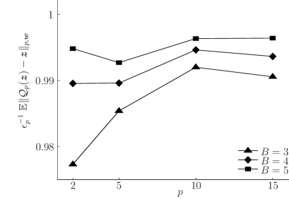
Figure 1: Comparing the theoretical bound $\epsilon_{p}$ to the empirical mean estimate of ${\mathbb{E}}\|\mathcal{Q}_{p}[\boldsymbol{z}]-\boldsymbol{z}\|_{p,\boldsymbol{w}}$ using 1000 trials of Monte-Carlo simulations, for each $B=3,4,5$).

Fig. 1 shows how well the $\epsilon_{p}$ estimates the distortion $\|\mathcal{Q}_{p}[\boldsymbol{z}]-\boldsymbol{z}\|_{p,\boldsymbol{w}}$ for the weights and the $p$-optimal levels given in Lemma 2. This has been measured by averaging this quantization distortion for 1000 realizations of a Gaussian random vector $\sim\mathcal{N}^{M}(0,1)$ with $M=2^{10}$, $p\in\{2,\,\cdots,15\}$ and $B=3,4$ and 5. We observe that the bias of $\epsilon_{p}$, as reflected here by the ratio $\epsilon_{p}^{-1}\,{\mathbb{E}}\|\mathcal{Q}_{p}[\boldsymbol{z}]-\boldsymbol{z}\|_{p,\boldsymbol{w}}$, is rather limited and decreases when $p$ and $B$ increase with a maximum relative error of about $2.5\%$ between the true and estimated distortion at $B=3$ and $p=2$.

Inspired by relation (13), we say that an estimate $\boldsymbol{x}^{*}\in\mathbb{R}^{N}$ of $\boldsymbol{x}$ sensed by the model (1) satisfies the $p$-Distortion Consistency (or D_pC) if

$$\|\boldsymbol{\Phi}\boldsymbol{x}^{*}-\mathcal{Q}_{p}[\boldsymbol{y}]\|_{p,\boldsymbol{w}}\ \leqslant\ \epsilon_{p},$$ (D_pC)

with the weights $w_{i}(p)=\mathcal{G}^{\prime}\big{(}\mathcal{Q}_{p}[y_{i}])^{(p-2)/p}$.

The class of D_pC constraints has QC and DC as its limit cases.

Lemma 4.

Given $\boldsymbol{y}=\mathcal{Q}[\boldsymbol{\Phi}\boldsymbol{x}]$, we have asymptotically in $B$

$${\rm D}_{2}{\rm C}\ \equiv\ {\rm DC}\qquad\text{and}\qquad{\rm D}_{\infty}{\rm C}\ \equiv\ {\rm QC}.$$

Proof.

Let $\boldsymbol{x}^{*}\in\mathbb{R}^{N}$ be a vector to be tested with the DC, QC or D_pC constraints. The first equivalence for $p=2$ is straightforward since $\boldsymbol{w}(2)=\boldsymbol{1}$, $\|\boldsymbol{\Phi}\boldsymbol{x}^{*}-\mathcal{Q}_{p}[\boldsymbol{y}]\|_{p,\boldsymbol{w}}=\|\boldsymbol{\Phi}\boldsymbol{x}^{*}-\mathcal{Q}[\boldsymbol{y}]\|_{2}$ and $\epsilon^{2}_{2}=\epsilon^{2}_{\rm DC}=\tfrac{2^{-2B}}{12}\,|\!|\!|\varphi_{0}|\!|\!|_{1/3}$ from (6).

For the second, we use the fact that $\boldsymbol{y}=\mathcal{Q}[\boldsymbol{\Phi}\boldsymbol{x}]$ is fixed by the sensing model (1). Let us denote by $k(i)$ the index of the bin to which $\mathcal{Q}_{p}[y_{i}]$ belongs for $1\leqslant i\leqslant M$. Since $\|\boldsymbol{\Phi}\boldsymbol{x}\|_{\infty}$ is fixed, and because relation (11) in Lemma 2 implies that the amplitude of the first or of the last $\Theta(B^{-1/2}2^{(1-\beta)B})$ thresholds grow faster than $T=\Theta(\sqrt{\beta B})$ for $0<\beta<1$, there exists necessarily a $B_{0}\geqslant 0$ such that $-T(B)\leqslant t_{k(i)}\leqslant t_{k(i)+1}\leqslant T(B)$ for all $B\geqslant B_{0}$ and all $1\leqslant i\leqslant M$.

Writing $\boldsymbol{W}_{\!\!p}=\operatorname{diag}(\boldsymbol{w}(p))$, we can use the equivalence $\|\cdot\|_{\infty}\leqslant\|\cdot\|_{p}\leqslant M^{1/p}\,\|\cdot\|_{\infty}$ and the squeeze theorem on the following limit:

$$\lim_{p\to\infty}\|\boldsymbol{\Phi}\boldsymbol{x}^{*}-\mathcal{Q}_{p}[\boldsymbol{y}]\|_{p,\boldsymbol{w}(p)}=\ \lim_{p\to\infty}\|\boldsymbol{W}_{\!\!p}\big{(}\Phi\boldsymbol{x}^{*}-\mathcal{Q}_{p}[\boldsymbol{y}]\big{)}\|_{p}\\ =\ \lim_{p\to\infty}\,\|\boldsymbol{W}_{\!\!p}\big{(}\Phi\boldsymbol{x}^{*}-\mathcal{Q}_{p}[\boldsymbol{y}]\big{)}\|_{\infty}.$$

Moreover, since for $B\geqslant B_{0}$ and for all $1\leqslant i\leqslant M$ the bin $\mathcal{R}_{k(i)}$ is finite, the limit

$$\lim_{p\to\infty}\,\mathcal{G}^{\prime}(\mathcal{Q}_{p}[y_{i}])^{(p-2)/p}\,\big{|}(\boldsymbol{\Phi}\boldsymbol{x}^{*})_{i}-\mathcal{Q}_{p}[y_{i}]\big{|}$$

exists and is finite. Therefore, from the continuity of the $\max$ function applied on the $M$ components of vectors in $\mathbb{R}^{M}$, we find

$$\lim_{p\to\infty}\|\boldsymbol{\Phi}\boldsymbol{x}^{*}-\mathcal{Q}_{p}[\boldsymbol{y}]\|_{p,\boldsymbol{w}(p)} =\ \lim_{p\to\infty}\,\max_{i}\,\mathcal{G}^{\prime}(\mathcal{Q}_{p}[y_{i}])^{(p-2)/p}\,\big{|}(\boldsymbol{\Phi}\boldsymbol{x}^{*})_{i}-\mathcal{Q}_{p}[y_{i}]\big{|}$$

$$=\ \max_{i}\,\lim_{p\to\infty}\ \mathcal{G}^{\prime}(\mathcal{Q}_{p}[y_{i}])^{(p-2)/p}\,\big{|}(\boldsymbol{\Phi}\boldsymbol{x}^{*})_{i}-\mathcal{Q}_{p}[y_{i}]\big{|}$$

$$=\ \max_{i}\,\mathcal{G}^{\prime}(\mathcal{Q}_{\infty}(y_{i}))\,\big{|}(\boldsymbol{\Phi}\boldsymbol{x}^{*})_{i}-\mathcal{Q}_{\infty}(y_{i})\big{|}.$$

For $B\geqslant B_{0}$, (10) provides $\mathcal{G}^{\prime}(\mathcal{Q}_{\infty}(y_{i}))\simeq_{B}\tfrac{\upalpha}{\uptau_{k(i)}}$, so that, if we impose $\lim_{p\to\infty}\|\boldsymbol{\Phi}\boldsymbol{x}^{*}-\mathcal{Q}_{p}[\boldsymbol{y}]\|_{p,\boldsymbol{w}(p)}\leqslant\epsilon_{\rm QC}=\upalpha/2$, we get asymptotically in $B$

$$\max_{i}{\textstyle\frac{1}{\uptau_{k(i)}}}\,\big{|}(\boldsymbol{\Phi}\boldsymbol{x}^{*})_{i}-\mathcal{Q}_{\infty}(y_{i})\big{|}\ \mathop{\lesssim}_{B}\ {\textstyle\frac{1}{2}},$$

which is equivalent to imposing $(\boldsymbol{\Phi}\boldsymbol{x}^{*})_{i}\in\mathcal{R}_{k(i)}$, i.e., the Quantization Constraint. ∎

III Weighted $\ell_{p}$ Fidelities in Compressed Sensing and General Reconstruction Guarantees

The last section has provided us some weighted $\ell_{p,\boldsymbol{w}}$ constraints, with appropriate weights $\boldsymbol{w}$, that can be used for stabilizing the reconstruction of a signal observed through the quantized sensing model (1). We now turn to studying the stability of $\ell_{1}$-based decoders integrating these weighted $\ell_{p,\boldsymbol{w}}$-constraints as data fidelity. We will highlight also the requirements that the sensing matrix must fulfill to ensure this stability. We then then apply this general stability result to additive heteroscedastic GGD noise, where weighing can be view as a variance stabilization transform. Section IV will later instantiate the outcome of this section to the particular case of QCS.

III-A Generalized Basis Pursuit DeNoise

Given some positive weights $\boldsymbol{w}\in\mathbb{R}^{M}$ and $p\geqslant 2$, we study the following general minimization program, coined General Basis Pursuit DeNoise (GBPDN),

$$\Delta_{p,\boldsymbol{w}}(\boldsymbol{y},\boldsymbol{\Phi},\epsilon)\ =\ \operatorname*{Argmin}_{\boldsymbol{u}\,\in\,\mathbb{R}^{N}}\|\boldsymbol{u}\|_{1}\ {\rm s.t.}\ \|\boldsymbol{y}-\boldsymbol{\Phi}\boldsymbol{u}\|_{p,\boldsymbol{w}}\leqslant\epsilon,$$

where $\|\!\cdot\!\|_{p,\boldsymbol{w}}$ is the weighted $\ell_{p}$-norm defined in the previous section. Note that BPDN is special case of GBPDN corresponding to $p=2$ and $\boldsymbol{w}=\boldsymbol{1}$. The Basis Pursuit DeQuantizers (BPDQ) introduced in [8] are associated to $p\geqslant 1$ and $\boldsymbol{w}=\boldsymbol{1}$, while the case $p=1$ and $\boldsymbol{w}=\boldsymbol{1}$ has also been covered in [20].

We are going to see that the stability of GBPDN$(\ell_{p,\boldsymbol{w}})$ is guaranteed if $\boldsymbol{\Phi}$ satisfies a particular instance of the following general isometry property.

Definition 1.

Given two normed spaces $\mathcal{X}=(\mathbb{R}^{M},\|\cdot\|_{\mathcal{X}})$ and $\mathcal{Y}=(\mathbb{R}^{N},\|\cdot\|_{\mathcal{Y}})$ (with $M<N$), a matrix $\boldsymbol{\Phi}\in\mathbb{R}^{M\times N}$ satisfies the Restricted Isometry Property from $\mathcal{X}$ to $\mathcal{Y}$ at order $K\in\mathbb{N}$, radius $0\leqslant\delta<1$ and for a normalization $\mu>0$, if for all $\boldsymbol{x}\in\Sigma_{K}$,

$$(1-\delta)^{1/\kappa}\,\|\boldsymbol{x}\|_{\mathcal{Y}}\leqslant{\textstyle\frac{1}{\mu}}\|\boldsymbol{\Phi}\boldsymbol{x}\|_{\mathcal{X}}\leqslant(1+\delta)^{1/\kappa}\,\|\boldsymbol{x}\|_{\mathcal{Y}},$$ (14)

$\kappa$ being an exponent function of the geometries of $\mathcal{X},\mathcal{Y}$. To lighten notation, we will write that $\boldsymbol{\Phi}$ is RIP${}_{\mathcal{X},\mathcal{Y}}(K,\delta,\mu)$.

We may notice that the common RIP is equivalent to RIP${}_{\ell_{2}^{M},\ell_{2}^{N}}(K,\delta,1)$ with $\kappa=1$, while the RIP_p,q introduced earlier in [8] is equivalent to RIP${}_{\ell_{p}^{M},\ell_{q}^{N}}(K,\delta,\mu)$ with $\kappa=q$ and $\mu$ depending only on $M$, $p$ and $q$. Moreover, the RIP${}_{p,K,\delta^{\prime}}$ defined in [21] is equivalent to the RIP${}_{\ell_{p}^{M},\ell_{p}^{N}}(K,\delta,\mu)$ with $\kappa=1$, $\delta^{\prime}=2\delta/(1-\delta)$ and $\mu=1/(1-\delta)$. Finally, the Restricted $p$-Isometry Property proposed in [22] is also equivalent to the RIP${}_{\ell_{p}^{M},\ell_{2}^{N}}(K,\delta,1)$ with $\kappa=p$.

In order to study the behavior of the GBPDN program, we are interested in the embedding induced by $\boldsymbol{\Phi}$ in (14) of $\mathcal{Y}=\ell_{2}^{N}$ into the normed space $\mathcal{X}=\ell_{p,\boldsymbol{w}}^{M}=(\mathbb{R}^{M},\|\!\cdot\!\|_{p,\boldsymbol{w}})$, i.e., we consider the RIP${}_{\ell_{p,\boldsymbol{w}}^{M},\,\ell_{2}^{N}}$ property that we write in the following as RIP_p,w. The following theorem establishes that GBPDN provides stable recovery from distorted measurements, if the RIP_p,w holds.

Theorem 1.

Let $K\geqslant 0$, $2\leqslant p<\infty$ and $\boldsymbol{\Phi}\in\mathbb{R}^{M\times N}$ be a RIP${}_{p,\boldsymbol{w}}(s,\delta_{s},\mu)$ matrix for $s\in\{K,2K,3K\}$ such that

$$\delta_{2K}+\sqrt{(1+\delta_{K})(\delta_{2K}+\delta_{3K})(p-1)}<1/3~{}.$$ (15)

Then, for any signal $\boldsymbol{x}\in\mathbb{R}^{N}$ observed according to the noisy sensing model $\boldsymbol{y}=\boldsymbol{\Phi}\boldsymbol{x}+\boldsymbol{\varepsilon}$ with $\|\boldsymbol{\varepsilon}\|_{p,\boldsymbol{w}}\leqslant\epsilon$, the unique solution $\boldsymbol{x}^{*}=\Delta_{p,\boldsymbol{w}}(\boldsymbol{y},\boldsymbol{\Phi},\epsilon)$ obeys

$$\|\boldsymbol{x}^{*}-\boldsymbol{x}\|\ \leqslant\ 4\,e_{0}(K)\ +\ 8\,\epsilon/\mu,$$ (16)

where $e_{0}(K)=K^{-\frac{1}{2}}\,\|\boldsymbol{x}-\boldsymbol{x}_{K}\|_{1}$ is the $K$-term $\ell_{1}$-approximation error.

Proof.

If $\boldsymbol{\Phi}$ is RIP${}_{p,\boldsymbol{w}}(s,\delta_{s},\mu)$ for $s\in\{K,2K,3K\}$, then, by definition of the weighted $\ell_{p,\boldsymbol{w}}$-norm, $\operatorname{diag}(\boldsymbol{w})\boldsymbol{\Phi}$ is RIP${}_{\ell_{p}^{M},\ell_{2}^{N}}(s,\delta_{s},\mu)$. Since $\Delta_{p,\boldsymbol{w}}(\boldsymbol{y},\boldsymbol{\Phi},\epsilon)\ =\Delta_{p}(\operatorname{diag}(\boldsymbol{w})\boldsymbol{y},\operatorname{diag}(\boldsymbol{w})\boldsymbol{\Phi},\epsilon)$, the stability results proved in [8, Theorem 2] for GBPDN$(\ell_{p})$ shows that

$$\|\boldsymbol{x}-\boldsymbol{x}^{*}\|\leqslant A_{p}\,e_{0}(K)+B_{p}\,\tfrac{\epsilon}{\mu},$$

with $A_{p}=\tfrac{2(1+C_{p}-\delta_{2K})}{1-\delta_{2K}-C_{p}}$, $B_{p}=\tfrac{4\sqrt{1+\delta_{2K}}}{1-\delta_{2K}-C_{p}}$ and $C_{p}\leqslant\sqrt{(1+\delta_{K})(\delta_{2K}+\delta_{3K})(p-1)}$ [8]. It is easy to see that if (15) holds, then $A_{p}\leqslant 4$ and $B_{p}\leqslant 8$. ∎

As we shall see shortly, this theorem may be used to characterize the impact of measurement corruption due to both additive heteroscedastic GGD noise (Section III-C) as well as those induced by a non-uniform scalar quantization (Section IV). Before detailing these two sensing scenarios, we first address the question of designing matrices satisfying the RIP_p,w for $2\leqslant p<\infty$.

III-B Weighted Isometric Mappings

We will describe a random matrix construction that will satisfy the RIP_p,w for $1\leqslant p<\infty$. To quantify when this is possible, we introduce some properties on the positive weights $\boldsymbol{w}$.

Definition 2.

A weight generator $\mathcal{W}$ is a process (random or deterministic) that associates to $M\in\mathbb{N}$ a weight vector $\boldsymbol{w}=\mathcal{W}(M)\in\mathbb{R}^{M}$. This process is said to be of Converging Moments (CM) if for $p\geqslant 1$ and all $M\geqslant M_{0}$ for a certain $M_{0}>0$,

$$\rho_{p}^{\min}\ \leqslant\ M^{-1/p}\,\|\mathcal{W}(M)\|_{p}\ \leqslant\ \rho_{p}^{\max},$$ (17)

where $\rho_{p}^{\min}>0$ and $\rho_{p}^{\max}>0$ are, respectively, the largest and the smallest values such that (17) holds. In other words, a CM generator $\mathcal{W}$ is such that $\|\mathcal{W}(M)\|^{p}_{p}=\Theta(M)$. By extension, we say that the weighting vector $\boldsymbol{w}$ has the CM property, if it is generated by some CM weight generator $\mathcal{W}$.

The CM property can be ensured if $\lim_{M\to\infty}M^{-1/p}\,\|\boldsymbol{w}\|_{p}$ exists, bounded and nonzero. It is also ensured if the weights $\{w_{i}\}_{1\leqslant i\leqslant M}$ are taken (with repetition) from a finite set of positive values. More generally, if $\{w_{i}:1\leqslant i\leqslant M\}$ are $\operatorname{iid}$ random variables, we have $M^{-1}\,\|\boldsymbol{w}\|^{p}_{p}={\mathbb{E}}|w_{1}|^{p}$ almost surely by the SLLN. Notice finally that $\rho^{\max}_{p}\leqslant\|\boldsymbol{w}\|_{\infty}=\rho^{\max}_{\infty}$ since $\|\boldsymbol{w}\|^{p}_{p}\leqslant M\|\boldsymbol{w}\|_{\infty}^{p}$, and $\rho^{\min}_{p}\geqslant\min_{i}|w_{i}|$.

For a weighting vector $\boldsymbol{w}$ having the CM property, we define also its weighting dynamic at moment $p$ as the ratio

$$\theta_{p}=\big{(}\tfrac{\rho^{\max}_{\infty}}{\rho_{p}^{\min}}\big{)}^{2}.$$

We will see later that $\theta_{p}$ directly influences the number of measurements required to guarantee the existence of RIP_p,w random Gaussian matrices.

Given a weight vector $\boldsymbol{w}$, the following lemma (proved in Appendix E) characterizes the expectation of the $\ell_{p,\boldsymbol{w}}$-norm of a random Gaussian vector.

Lemma 5 (Gaussian $\ell_{p,w}$-Norm Expectation).

If $\boldsymbol{\xi}\sim\mathcal{N}^{M}(0,1)$ and if the weights $\boldsymbol{w}$ have the CM property, then, for $1\leqslant p<\infty$ and $\mathcal{Z}\sim\mathcal{N}(0,1)$,

$$\big{(}1\ +\ 2^{p+1}\,\theta_{p}^{p}\,M^{-1}\big{)}^{\frac{1}{p}-1}\,({\mathbb{E}}\|\boldsymbol{\xi}\|_{p,\boldsymbol{w}}^{p})^{\frac{1}{p}}\ \leqslant\ {\mathbb{E}}\|\boldsymbol{\xi}\|_{p,\boldsymbol{w}}\ \leqslant\ ({\mathbb{E}}\|\boldsymbol{\xi}\|_{p,\boldsymbol{w}}^{p})^{\frac{1}{p}}=({\mathbb{E}}|\mathcal{Z}|^{p})^{1/p}\|\boldsymbol{w}\|_{p}.$$

In particular, ${\mathbb{E}}\|\boldsymbol{\xi}\|_{p,\boldsymbol{w}}\simeq_{M}\nu_{p}\,\|\boldsymbol{w}\|_{p}\geqslant\nu_{p}\,M^{1/p}\,\rho_{p}^{\min}$, with $\nu_{p}^{p}:={\mathbb{E}}|\mathcal{Z}|^{p}=2^{p/2}\pi^{-1/2}\Gamma(\tfrac{p+1}{2})$.

With an appropriate modification of [8, Proposition 1], we can now prove the existence of random Gaussian RIP_p,w matrices (see Appendix F).

Proposition 1 (RIP_p,w Matrix Existence).

Let $\boldsymbol{\Phi}\sim\mathcal{N}^{M\times N}(0,1)$ and some CM weights $\boldsymbol{w}\in\mathbb{R}^{M}$. Given $p\geqslant 1$ and $0\leqslant\eta<1$, then there exists a constant $c>0$ such that $\boldsymbol{\Phi}$ is RIP${}_{p,\boldsymbol{w}}(K,\delta,\mu)$ with probability higher than $1-\eta$ when we have jointly $M\geqslant 2\,(2\theta_{p})^{p}$, and

$$M^{2/\!\max(2,\,p)} \geqslant c\,\delta^{-2}\,\theta_{p}\,\big{(}K\log[e\tfrac{N}{K}(1+12\delta^{-1})]\ +\ \log\tfrac{2}{\eta}\big{)}.$$ (18)

Moreover, the value $\mu=\mu(\ell_{p,\boldsymbol{w}}^{M},\ell^{N}_{2})$ in (14) is given by $\mu={\mathbb{E}}\|\boldsymbol{\xi}\|_{p,\boldsymbol{w}}$ for a random vector $\boldsymbol{\xi}\sim\mathcal{N}^{M}(0,1)$.

The RIP normalizing constant $\mu$ can be bounded owing to Lemma 5.

Remark 2.

In the light of Proposition 1, assumption (15) becomes reasonable since following the simple argument presented in [8, Appendix B] the saturation of requirement (18) implies that $\delta_{K}$ decays as $O(\sqrt{K\log M}/M^{1/p})$ for RIP_p,w Gaussian matrices. Therefore, for any value $p$, it is always possible to find a $M$ such that (15) holds. However, this is only possible for high oversampling situation, i.e., for $\Omega((K\log N/K)^{p/2})$ measurements.

III-C GBPDN stabilizes Heteroscedastic GGD Noise

Consider the following general signal sensing model

$$\boldsymbol{y}\ =\ \boldsymbol{\Phi}\boldsymbol{x}\ +\ \boldsymbol{\varepsilon}~{},$$ (19)

where $\boldsymbol{\varepsilon}\in\mathbb{R}^{M}$ is the noise vector. For heteroscedastic GGD noise, each $\varepsilon_{i}$ follows a zero-mean ${\rm GGD}(0,\alpha_{i},p)$ distribution with pdf $\propto\exp(-|t/\alpha_{i}|^{p})$, where $p>0$ is the shape parameter (the same for all $\varepsilon_{i}$’s), and $\alpha_{i}>0$ the scale parameter [23]. It is obvious that

$${\mathbb{E}}\boldsymbol{\varepsilon}=\boldsymbol{0}\quad\text{and}\quad{\mathbb{E}}(\boldsymbol{\varepsilon}\boldsymbol{\varepsilon}^{\mathrm{T}})=\Gamma(3/p)(\Gamma(1/p))^{-1}\operatorname{diag}(\alpha_{1}^{2},\,\cdots,\alpha_{M}^{2}).$$

If one sets the weights to $w_{i}=1/\alpha_{i}$ in GBPDN$(\ell_{p,\boldsymbol{w}})$, it can be seen that the associated constraint corresponds precisely to the negative log-likelihood of the joint pdf of $\boldsymbol{\varepsilon}$. As detailed below, introducing these non-uniform weights $w_{i}$ leads to a reduction in the error of the reconstructed signal, relative to using constant weights. Without loss of generality, we here restrict our analysis to strictly $K$-sparse $\boldsymbol{x}\in\Sigma_{K}$, and assume knowledge of bounds (estimators) for the $\ell_{p}$ and the $\ell_{p,\boldsymbol{w}}$ norms used for characterizing $\boldsymbol{\varepsilon}$, i.e., we know that $\|\boldsymbol{\varepsilon}\|_{p}\simeq_{M}\epsilon$ and $\|\boldsymbol{\varepsilon}\|_{p,\boldsymbol{w}}\simeq_{M}\epsilon_{\rm st}$ for some $\epsilon,\epsilon_{\rm st}>0$ to be detailed later.

In this case, if the random matrix $\boldsymbol{\Phi}\sim\mathcal{N}^{M\times N}(0,1)$ is RIP${}_{p,\boldsymbol{w}}(K,\delta,\mu)$ for $p\geqslant 2$, with $\mu={\mathbb{E}}\|\boldsymbol{\xi}\|_{p}$ for $\boldsymbol{\xi}\sim\mathcal{N}^{M}(0,1)$, Theorem 1 asserts that

$$\|\boldsymbol{x}^{*}-\boldsymbol{x}\|\ \leqslant\ B_{p}\,\epsilon/\mu,$$

for $\boldsymbol{x}^{*}=\Delta_{p,\boldsymbol{1}}(\boldsymbol{y},\boldsymbol{\Phi},\epsilon)$ and $B_{p}\simeq_{M}8$. Conversely, for the weights to $w_{i}=1/\alpha_{i}$, and assuming $\boldsymbol{\Phi}$ being RIP${}_{p,\boldsymbol{w}}(K,\delta^{\prime},\mu_{\rm st})$ with $\mu_{\rm st}={\mathbb{E}}\|\boldsymbol{\xi}\|_{p,\boldsymbol{w}}$, we get

$$\|\boldsymbol{x}^{*}_{\rm st}-\boldsymbol{x}\|\ \leqslant\ B^{\prime}_{p}\,\epsilon_{\rm st}/\mu_{\rm st},$$

for $\boldsymbol{x}^{*}_{\rm st}=\Delta_{p,\boldsymbol{w}}(\boldsymbol{y},\boldsymbol{\Phi},\epsilon)$ and $B^{\prime}_{p}\simeq_{M}8$.

When the number of measurements $M$ is large, using classical GGD absolute moments formula, the two bounds $\epsilon$ and $\epsilon_{\rm st}$ can be set close to $\epsilon^{p}\mathop{\simeq}_{M}\sum_{i}{\mathbb{E}}|\varepsilon_{i}|^{p}=\|\boldsymbol{\alpha}\|_{p}^{p}/p$ and $\epsilon_{\rm st}^{p}\mathop{\simeq}_{M}\sum_{i}w_{i}^{p}\,{\mathbb{E}}|\varepsilon_{i}|^{p}=M/p$. Moreover, using Lemma 5, $\mu^{p}\mathop{\simeq}_{M}\sum_{i}{\mathbb{E}}|\xi_{i}|^{p}=M{\mathbb{E}}|\mathcal{Z}|^{p}$ and $\mu_{\rm st}^{p}\mathop{\simeq}_{M}{\mathbb{E}}|\mathcal{Z}|^{p}\,\|\boldsymbol{w}\|^{p}_{p}$, where $\mathcal{Z}\sim\mathcal{N}(0,1)$.

Proposition 2.

For an additive heteroscedastic noise $\boldsymbol{\varepsilon}\in\mathbb{R}^{M}$ such that $\varepsilon_{i}\sim_{\rm iid}{\rm GGD}(0,\alpha_{i},p)$, setting $w_{i}=1/\alpha_{i}$ provides $\epsilon_{\rm st}^{p}/\mu_{\rm st}^{p}\ \lesssim_{M}\ \epsilon^{p}/\mu^{p}$. Therefore, asymptotically in $M$, GBPDN$(\ell_{p,\boldsymbol{w}})$ has a smaller reconstruction error compared to GBPDN$(\ell_{p})$ when estimating $\boldsymbol{x}$ from the sensing model (19).

Proof.

Let us observe that $\epsilon_{\rm st}^{p}/\mu_{\rm st}^{p}\simeq_{M}M(p\,{\mathbb{E}}|\mathcal{Z}|^{p}\,\|\boldsymbol{w}\|^{p}_{p})^{-1}=(p\,{\mathbb{E}}|\mathcal{Z}|^{p})^{-1}({\textstyle\frac{1}{M}}\sum_{i}{\textstyle\frac{1}{\alpha_{i}^{p}}})^{-1}$. By the Jensen inequality, $({\textstyle\frac{1}{M}}\sum_{i}{\textstyle\frac{1}{\alpha_{i}^{p}}})^{-1}\leqslant{\textstyle\frac{1}{M}}\sum_{i}\alpha_{i}^{p}$, so that $\epsilon_{\rm st}^{p}/\mu_{\rm st}^{p}\lesssim_{M}{\textstyle\frac{1}{p}}\,({\mathbb{E}}|\mathcal{Z}|^{p})^{-1}\|\boldsymbol{\alpha}\|^{p}_{p}/M=\epsilon^{p}/\mu^{p}$. ∎

The price to pay for this stabilization is an increase of the weighting dynamic $\theta_{p}=(\tfrac{\rho^{\max}_{\infty}}{\rho^{\min}_{p}})^{2}$ defined in Proposition 1, which implies an increase in the number of measurements $M$ needed to ensure that the RIP${}_{p,\boldsymbol{w}}(K,\delta,\mu)$ is satisfied.

Example.

Let us consider a simple situation where the $\alpha_{i}$’s take only two values, i.e., $\alpha_{i}\in\{1,H\}$ for some $H\geqslant 1$. Let us assume also that the proportion of $\alpha_{i}$’s equal to $H$ converges to $r\in[0,1]$ with $M$ as $|\frac{1}{M}\#\{i:\alpha_{i}=H\}\ -\ r|=O(M^{-1})$. In this case, the stabilizing weights are $w_{i}=1/\alpha_{i}\in\{1,1/H\}$. An easy computation provides

$$\mathsf{E} :=\tfrac{\epsilon^{p}}{\mu^{p}}\ \mathop{\simeq}_{M}\ {\textstyle\frac{1}{p}}\nu_{p}^{-p}\,\big{(}\,r\,H^{p}+(1-r)\,\big{)},$$

$$\mathsf{E}_{\rm st} :=\tfrac{\epsilon_{\rm st}^{p}}{\mu_{\rm st}^{p}}\ \mathop{\simeq}_{M}\ {\textstyle\frac{1}{p}}\nu_{p}^{-p}\,\big{(}\,r\,H^{-p}+(1-r)\,\big{)}^{-1},$$

so that, the “stabilization gain” with respect to an unstabilized setting can be quantified by the ratio

$$(\tfrac{\mathsf{E}}{\mathsf{E}_{\rm st}})^{\frac{1}{p}}\ {\mathop{\simeq}_{M}}\ \big{(}\,r\,H^{-p}+(1-r)\,\big{)}^{\frac{1}{p}}\big{(}\,r\,H^{p}+(1-r)\,\big{)}^{\frac{1}{p}}\ {\mathop{\simeq}_{M,H}}\ \big{(}r\,(1-r)\big{)}^{\frac{1}{p}}\,H.$$

We see that the stabilization provides a clear gain which increases as the measurements get very unevenly corrupted, i.e., when $H$ is large. Interestingly, the higher $p$ is, the less sensitive is this gain to $r$. We also observe that the overhead in the number of measurements between the stabilized and the unstabilized situations is related to

$$\theta^{p/2}_{p}\ =\big{(}\tfrac{\rho^{\max}_{\infty}}{\rho^{\min}_{p}}\big{)}^{p}\ {\mathop{\simeq}_{M}}\ \big{(}\,r\,H^{-p}+(1-r)\,\big{)}^{-1}\ {\mathop{\simeq}_{M,H}}\ (1-r)^{-1}.$$

The limit case where $H\gg 1$ can be interpreted as ignoring $r$ percent of the measurements in the data fidelity constraint, keeping only those for which the noise is not dominating. In that case, the sufficient condition (18) in Proposition 1 for $\boldsymbol{\Phi}$ to be RIP_p,w tends to $\theta_{p}^{-p/2}M=(1-r)M=\Omega\big{(}(K\log N/K)^{p/2}\big{)}$ which is consistent with the fact that on average only fraction $1-r$ of the $M$ measurements significantly participate to the CS scheme, i.e., $M^{\prime}=(1-r)M$ must satisfy the common RIP requirement. For $p=2$, this is somehow related to the democratic property of RIP matrices [4], i.e., the fact that a reasonable number of rows can be discarded from a matrix while preserving the RIP. This property was successfully used for discarding saturated CS measurements in the case of a limited dynamic quantizer [4].

IV Dequantizing with Generalized Basis Pursuit DeNoise

Let us now instantiate the use of GBPDN to the reconstruction of signals in the QCS scenario defined in SectionII. Under the quantization formalism defined in Lemma 3 and for Gaussian matrices $\boldsymbol{\Phi}$, the factor $\epsilon/\mu$ in (16) can be shown to decrease as $1/\sqrt{p+1}$ asymptotically in $M$ and $B$. This asymptotic and almost sure result which relies on the SLLN (see Appendix G) suggests increasing $p$ to the highest value allowed by (15) in order to decrease the GBPDN reconstruction error.

Proposition 3 (Dequantizing Reconstruction Error).

Given $\boldsymbol{x}\in\mathbb{R}^{N}$ and $\boldsymbol{\Phi}\sim\mathcal{N}^{M\times N}(0,1)$, assume that the entries of $\boldsymbol{z}=\boldsymbol{\Phi}\boldsymbol{x}$ are $\operatorname{iid}$ realizations from $\mathcal{Z}\sim\mathcal{N}(0,\sigma_{0}^{2})$. We take the corresponding optimal compressor function $\mathcal{G}$ defined in (3) and the $p$-optimal $B$-bits scalar quantizer $\mathcal{Q}_{p}$ as defined in (8). Then, the ratio ${\epsilon}/{\mu}$ given in (16) is asymptotically and almost surely bounded by

$$\tfrac{\epsilon}{\mu}\ \lesssim_{B,M}\ c^{\prime}\,2^{-B}\,\,\tfrac{(p+1)^{-\frac{1}{2p}}}{\sqrt{p+1}}\leqslant c^{\prime}\,\frac{2^{-B}}{\sqrt{p+1}}.$$

with $c^{\prime}=(9/8)(e\pi/3)^{1/2}$.

Notice that, under HRA and for large $M$, it is possible to provide a rough estimation of the weighting dynamic $\theta_{p}$ when the weights are those provided by the D_pC constraints. Indeed, since $w_{i}(p)=\mathcal{G}^{\prime}(\mathcal{Q}_{p}[y_{i}])^{(p-2)/p}$ and $\mathcal{G}^{\prime}=\gamma_{0,\sqrt{3}\sigma_{0}}$, we find

$$\|\boldsymbol{w}\|^{p}_{p} =\sum_{i}\mathcal{G}^{\prime}(\mathcal{Q}_{p}[y_{i}])^{p-2}\ \simeq_{M}\ M\,\sum_{k}\mathcal{G}^{\prime p-2}(\omega_{k,p})\,p_{k}$$

$$\simeq_{B,M}\,M\,(2\pi 3\sigma_{0}^{2})^{(2-p)/2}(2\pi\sigma_{0}^{2})^{-1/2}\sum_{k}\uptau_{k}\,\exp(-{\textstyle\frac{1}{2}}\omega_{k,p}^{2}\tfrac{p+1}{3\sigma^{2}_{0}})$$

$$\simeq_{B,M}\,M\,(2\pi 3\sigma_{0}^{2})^{(2-p)/2}(2\pi\sigma_{0}^{2})^{-1/2}(2\pi\tfrac{3\sigma_{0}^{2}}{p+1})^{1/2}$$

$$=\ M\,(2\pi\sigma_{0}^{2})^{(2-p)/2}3^{(3-p)/2}(p+1)^{-1/2},$$

where we recall that $p_{k}=\int_{\mathcal{R}_{k}}\varphi_{0}(t)\mathrm{d}t\simeq_{B}\varphi_{0}(c^{\prime})\uptau_{k}$, for any $c^{\prime}\in\mathcal{R}_{k}$ (see the proof of Lemma 9).

Moreover, using (10) and since one of the two smallest quantization bins is $\mathcal{R}_{\mathcal{B}/2}=[0,\tau_{\mathcal{B}/2})$,

$$\|\boldsymbol{w}\|^{p}_{\infty}\simeq_{B}(\upalpha/\uptau_{\mathcal{B}/2})^{p-2}=(\upalpha/\mathcal{G}^{-1}(1/2+\upalpha))^{p-2}\simeq_{B}(2\pi 3\sigma_{0}^{2})^{(2-p)/2}.$$

Therefore, estimating $\theta_{p}^{p}$ with $M^{2}\|\boldsymbol{w}\|^{2p}_{\infty}/\|\boldsymbol{w}\|^{2p}_{p}$, we find

$$\theta_{p}^{p/2}\ \simeq_{B,M}\ \sqrt{(p+1)/3}.$$

Therefore, at a given $p\geqslant 2$, since (18) involves that $M$ evolves like $\Omega(\theta_{p}^{p/2}(K\log N/K)^{p/2})$, using the weighting induced by GBPDN($\ell_{p,\boldsymbol{w}}$) requires collecting $\sqrt{(p+1)/3}$ times more measurements than GBPDN($\ell_{p}$) in order to ensure the appropriate RIP_p,w property. This represents part of the price to pay for guaranteeing bounded reconstruction error by adapting to non-uniform quantization.

Dequantizing is Stabilizing Quantization Distortion:

In connection with the procedure developed in Section III-C, the weights and the $p$-optimal levels introduced in Lemma 3 can be interpreted as a “stabilization” of the quantization distortion seen as a heteroscedastic noise. This means that, asymptotically in $M$, selecting these weights and levels, all quantization regions $\mathcal{R}_{k}$ contribute equally to the $\ell_{p,{\boldsymbol{w}}}$ distortion measure.

To understand this fact, we start by studying the following relation shown in the proof of Lemma 3 (see Appendix D):

$$\|\mathcal{Q}_{p}[\boldsymbol{z}]-\boldsymbol{z}\|^{p}_{p,\boldsymbol{w}}\ \mathop{\simeq}_{M}\ M\,\sum_{k}\ [\mathcal{G}^{\prime}(\omega_{k,p})]^{p-2}\int_{\mathcal{R}_{k}}|t-\omega_{k,p}|^{p}\,\varphi_{0}(t)\,\mathrm{d}t.$$ (20)

Using the threshold $T(B)=\Theta(\sqrt{B})$ and $\mathcal{T}=[-T(B),T(B)]$ as defined in Lemma 2, the proof of Lemma 9 in Appendix D shows that

$$\|\mathcal{Q}_{p}[\boldsymbol{z}]-\boldsymbol{z}\|^{p}_{p,\boldsymbol{w}}\ \mathop{\simeq}_{M,B}\ M\,\sum_{k:\mathcal{R}_{k}\subset\mathcal{T}}\ [\mathcal{G}^{\prime}(\omega_{k,p})]^{p-2}\int_{\mathcal{R}_{k}}|t-\omega_{k,p}|^{p}\,\varphi_{0}(t)\,\mathrm{d}t,$$ (21)

$$\mathop{\simeq}_{B}\ M\,\sum_{k:\mathcal{R}_{k}\subset\mathcal{T}}\ [\mathcal{G}^{\prime}(\omega_{k,p})]^{p-2}\tfrac{\uptau_{k}^{p+1}}{(p+1)\,2^{p}}\,\varphi_{0}(\omega_{k,p}),$$ (22)

using (9). However, using (10) and the relation $\mathcal{G}^{\prime}=\varphi_{0}^{1/3}/|\!|\!|\varphi_{0}|\!|\!|^{1/3}_{1/3}$, we find $\uptau^{3}_{k}\,\varphi_{0}(\omega_{k,p})\simeq_{B}\upalpha^{3}\,|\!|\!|\varphi_{0}|\!|\!|_{1/3}$. Therefore, each term of the sum in (21) provides a contribution

$$[\mathcal{G}^{\prime}(\omega_{k,p})]^{p-2}\tfrac{\uptau_{k}^{p+1}}{(p+1)\,2^{p}}\,\varphi_{0}(\omega_{k,p})\ \mathop{\simeq}_{B,M}\ |\!|\!|\varphi_{0}|\!|\!|_{1/3}\,\tfrac{\upalpha^{p+1}}{(p+1)2^{p}},$$

which is independent of $k$! This phenomenon is well known for $p=2$ and may actually serve for defining $\mathcal{G}^{\prime}$ itself [9]. The fact that this effect is preserved for $p\geqslant 2$ is a surprise for us.

V Numerical Experiments

We first describe how to numerically solve the GBPDN optimization problem using a primal-dual convex optimization scheme, then illustrate the use of GBPDN for stabilizing heteroscedastic Gaussian noise on the CS measurements. Finally, we apply GBPDN for reconstructing signals in the quantized CS scenario described in Section II.

V-A Solving GBPDN

The optimization problem GBPDN$(\ell_{p,\boldsymbol{w}})$ is a special instance of the general form

$$\min_{\boldsymbol{u}\in\mathbb{R}^{N}}f(\boldsymbol{u})+g({\boldsymbol{L}\boldsymbol{u}})~{},$$ (23)

where $f$ and $g$ are closed convex functions that are not infinite everywhere (i.e., proper functions), and $\boldsymbol{L}=\operatorname{diag}(\boldsymbol{w})\boldsymbol{\Phi}$ is a bounded linear operator, with $f(\boldsymbol{u}):=\|\boldsymbol{u}\|_{1}$, and $g(\boldsymbol{v}):=\imath_{{\mathbb{B}}_{p}^{\epsilon}}(\boldsymbol{v}-\boldsymbol{y})$ where $\imath_{{\mathbb{B}}_{p}^{\epsilon}}(\boldsymbol{v})$ is the indicator function of the $\ell_{p}$-ball ${\mathbb{B}}_{p}^{\epsilon}$ centered at zero and of radius $\epsilon$, i.e., $\imath_{{\mathbb{B}}_{p}^{\epsilon}}(\boldsymbol{v})=0$ if $\boldsymbol{v}\in{\mathbb{B}}_{p}^{\epsilon}$ and $+\infty$ otherwise. For the case of GBPDN$(\ell_{p,\boldsymbol{w}})$, both $f$ and $g$ are non-smooth but the associated proximity operators (to be defined shortly) can be computed easily. This will allow to minimize the GBPDN$(\ell_{p,\boldsymbol{w}})$ objective by calling on proximal splitting algorithms.

Before delving into the details of the minimization splitting algorithm, we recall some results from convex analysis. The proximity operator [24] of a proper closed convex $f$ is defined as the unique solution

$$\operatorname{prox}_{f}(\boldsymbol{u})=\operatorname*{argmin}_{\boldsymbol{z}}{\textstyle\frac{1}{2}}\|\boldsymbol{z}-\boldsymbol{u}\|^{2}+f(\boldsymbol{z}).$$

If $f=\imath_{C}$ for some closed convex set $C$, $\operatorname{prox}_{f}$ is equivalent to the orthogonal projector onto $C$, $\operatorname{proj}_{C}$. $f^{*}$ is the Legendre-Fenchel conjugate of $f$. For $\lambda>0$, the proximity operator of $\lambda f^{*}$ can be deduced from that of $f/\lambda$ through Moreau’s identity

$$\operatorname{prox}_{\lambda f^{*}}(\boldsymbol{u})=\boldsymbol{u}-\lambda\operatorname{prox}_{\lambda^{-1}f}(\boldsymbol{u}/\lambda)~{}.$$

Solving (23) with an arbitrary bounded linear operator $\boldsymbol{L}$ can be achieved using primal-dual methods motivated by the classical Kuhn-Tucker theory. Starting from methods to solve saddle function problems such as the Arrow-Hurwicz method [25], this problem has received a lot of attention recently, e.g., [26, 27, 28]. In this paper, we use the relaxed Arrow-Hurwicz algorithm as revitalized recently in [27]. Adapted to our problem, its steps are summarized in Algorithm V.1.

Inputs: Measurements $\boldsymbol{y}$, sensing matrix $\boldsymbol{\Phi}$, weights $\boldsymbol{w}$.

Parameters: Iteration number $N_{\mathrm{iter}}$, $\theta\in[0,1]$, step-sizes $\sigma>0$ and $\tau>0$ with $\tau\sigma\|\boldsymbol{w}\|_{\infty}^{2}\|\boldsymbol{\Phi}\|^{2}<1$.

Main iteration:

for $k=0$ to $N_{\mathrm{iter}}-1$ do

      

• Update the dual variable:

  $${\boldsymbol{v}}_{k+1}=\operatorname{prox}_{\sigma g^{*}}({\boldsymbol{v}}_{k}+\sigma{\boldsymbol{L}}\overline{\boldsymbol{u}}_{k})~{}.$$

• Update the primal variable:

  $${\boldsymbol{u}}_{k+1}=\operatorname{prox}_{\tau f}({\boldsymbol{u}}_{k}-\tau{\boldsymbol{L}}^{\mathrm{T}}{\boldsymbol{v}}_{k+1})~{}.$$

• Approximate extragradient step:

  $$\overline{\boldsymbol{u}}_{k+1}={\boldsymbol{u}}_{k+1}+\theta({\boldsymbol{u}}_{k+1}-{\boldsymbol{u}}_{k})~{}.$$

Output: Signal $\boldsymbol{u}_{N_{\mathrm{iter}}}$.

Algorithm V.1 Primal-dual scheme for solving GBPDN$(\ell_{p,\boldsymbol{w}})$.

A sufficient condition for the sequences of Algorithm V.1 to converge is to choose $\sigma$ and $\tau$ such that $\tau\sigma\|\boldsymbol{w}\|_{\infty}^{2}\|\boldsymbol{\Phi}\|^{2}<1$. It has been shown in [27, Theorem 1] that under this condition and for $\theta=1$, the primal sequence $(\boldsymbol{u}_{k})_{k\in\mathbb{N}}$ converges to a (possibly strict) global minimizer of GBPDN$(\ell_{p,\boldsymbol{w}})$, with the rate $O(1/k)$ in ergodic sense on the partial duality gap.

Proximity operator of $f$

For $f(\boldsymbol{u})=\|\boldsymbol{u}\|_{1}$, $\operatorname{prox}_{\tau f}(\boldsymbol{u})$ is the popular component-wise soft-thresholding of $\boldsymbol{u}$ with threshold $\tau$.

Proximity operator of $g$

Recall that $g(\boldsymbol{v})=\imath_{{\mathbb{B}}_{p}^{\epsilon}}(\boldsymbol{v}-\boldsymbol{y})$. Using Moreau’s identity above, and proximal calculus rules for translation and scaling, we have

$$\operatorname{prox}_{\sigma g^{*}}(\boldsymbol{v})={\boldsymbol{v}}-\sigma{\boldsymbol{y}}-\operatorname{proj}_{\imath_{{\mathbb{B}}_{p}^{\sigma\epsilon}}}(\boldsymbol{v}-\sigma\boldsymbol{y})~{}.$$

It remains to compute the orthogonal projection $\operatorname{proj}_{{\mathbb{B}}^{1}_{p}}$ to get $\operatorname{proj}_{{\mathbb{B}}^{\sigma\epsilon}_{p}}=\sigma\epsilon\operatorname{proj}_{{\mathbb{B}}^{1}_{p}}(\cdot/(\sigma\epsilon))$. For $p=2$ and $p=+\infty$, this projector has an easy closed form. For $2<p<+\infty$, we used the Newton method we proposed in [8] for solving the related Karush-Kuhn-Tucker system which is reminiscent of the strategy underlying sequential quadratic programming.

V-B Gaussian Noise Stabilization Illustration

We explore numerically the impact of using non-uniform weights (e.g., stabilizing the measurement noise) for signal reconstruction when the CS measurements are corrupted by heteroscedastic Gaussian noise, as discussed in Section III-C. This illustrates for $p=2$ both the gain induced by stabilizing the sensing noise and the increase of measurements necessary for observing this gain.

In this illustration, we set the problem dimensions to $N=1024$, $K=16$, and let the oversampling factor be in $M/K\in\{5,10,\cdots,50\}$. The $K$-sparse unit norm signals were generated independently according to a Bernoulli-Gaussian mixture model with $K$-length support picked uniformly at random in $[N]$, and the non-zero signal entries drawn from $\mathcal{N}(0,\sigma_{s}^{2})$ with $\sigma_{s}^{2}\simeq 1/K$. Noisy measurements were simulated by setting $\boldsymbol{y}=\boldsymbol{\Phi}\boldsymbol{x}+\boldsymbol{\varepsilon}$, with $\varepsilon_{i}\sim_{\operatorname{iid}}\mathcal{N}(0,\sigma_{i}^{2})$ and $\boldsymbol{\Phi}\sim\mathcal{N}^{M\times N}(0,1)$. The heteroscedastic behavior of $\boldsymbol{\varepsilon}$ has been designed so that $\sigma_{i}\sim_{\operatorname{iid}}\mathcal{U}([\sigma_{0}-\delta_{0},\sigma_{0}+\delta_{0}])$ with $\sigma_{0}=0.1$ and $\delta_{0}=0.6\,\sigma_{0}$.

Two reconstruction methods were tested: one with and the other without stabilizing the noise variance. In the first case, the weights have been set to $w_{i}=1/\sigma_{i}$, while in the second $\boldsymbol{w}=\boldsymbol{1}$. Since the purpose of this analysis is not focused on the design of efficient noise power estimators, $\epsilon$ and $\epsilon_{\rm st}$ have been simply set by an oracle to $\epsilon_{\rm st}=\|\boldsymbol{y}-\boldsymbol{\Phi}\boldsymbol{x}\|_{2,\boldsymbol{w}}$ and $\epsilon=\|\boldsymbol{y}-\boldsymbol{\Phi}\boldsymbol{x}\|_{2}$.

Given the parameters above, we compute the weighting dynamic $\theta_{p}\simeq_{M}\frac{M\,{\mathbb{E}}\|\boldsymbol{w}\|^{2}_{\infty}}{{\mathbb{E}}\|\boldsymbol{w}\|^{2}_{2}}=\frac{\sigma_{0}+\delta_{0}}{\sigma_{0}-\delta_{0}}=4$, and the average stabilization gain should be (see Proposition 2)

$$20\log_{10}\|\boldsymbol{x}-\boldsymbol{x}^{*}\|/\|\boldsymbol{x}-\boldsymbol{x}^{*}_{\rm st}\|\ \simeq_{M}\ 20\log_{10}(\epsilon\|\boldsymbol{w}\|)/(\epsilon_{\rm st}\sqrt{M})\ <2.43\,\text{dB}.$$

Numerically, GBPDN$(\ell_{2,\boldsymbol{w}})$ and GBPDN$(\ell_{2})\equiv\$BPDN have been solved with the method described in Section V-B until the relative $\ell_{2}$-change in the iterates was smaller than $10^{-6}$ (with a maximum of 2000 iterations). Reconstruction results were averaged over 50 experiments. In Fig. 2(a), the reconstruction signal-to-noise ratio (SNR) of the stabilized reconstruction is clearly superior to the unstabilized one and this gain increases with increasing oversampling ratio $M/K$. This SNR gain is displayed in Fig. 2(b). The dashed horizontal line represents the theoretical prediction of $2.43$ dB which turns to be an upper-bound on the numerically observed gain.

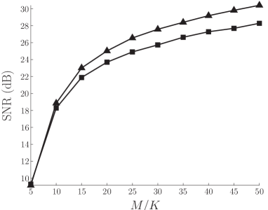
(a)

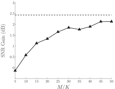
(b)

Figure 2: Stabilized versus unstabilized reconstruction using GBPDN$(\ell_{2,\boldsymbol{w}})$ and BPDN respectively. (a) The reconstruction SNR using stabilized (triangles) and unstabilized (squares) methods. (b) Observed (triangles) and theoretically predicted (dashed) SNR gain at $2.43$ dB brought by stabilization.

V-C Non-Uniform Quantization

We describe several simulations challenging the power of GBPDN for reconstructing sparse signals from non-uniformly quantized measurements when the weights and the $p$-optimal levels of Lemma 3 are combined. Several configurations have been tested for different $p\geqslant 2$, oversampling ratio $M/K$, number of bits $B$ and for non-uniform and uniform quantization.

For this experiment, we set the key dimensions to $N=1024,K=16,B=4$, and the $K$-sparse unit norm signals have been generated as in the previous section. The oversampling ratio was taken as $M/K\in\{10,15,\,\cdots,45\}$, $p\in\{2,4,\cdots,10\}$ and the matrix $\boldsymbol{\Phi}$ has been drawn randomly as $\boldsymbol{\Phi}\sim\mathcal{N}^{M\times N}(0,1)$. The non-uniform quantization of the measurements $\boldsymbol{\Phi}\boldsymbol{x}$ was defined with a compressor $\mathcal{G}$ associated to $\gamma_{0,\sigma_{0}}$ according to (3). The weights $\boldsymbol{w}$ were computed as in Lemma 3, and the $p$-optimal levels using the numerical method described in Appendix H.

For the sake of completeness, we also compared some results to those obtained for a uniformly quantized CS scenario. In this case, the measurements $\boldsymbol{z}=\boldsymbol{\Phi}\boldsymbol{x}$ are quantized as $y_{i}=\upalpha^{\prime}\lfloor z_{i}/\upalpha^{\prime}\rfloor+\upalpha^{\prime}/2$, the quantization bin width $\upalpha^{\prime}=\upalpha^{\prime}(B)$ has been set by dividing regularly the interval $[-\|\boldsymbol{z}\|_{\infty},\|\boldsymbol{z}\|_{\infty}]$ into the same number of bins as those used for the non-uniform quantization.

Again, GBPDN was solved with the primal-dual scheme described in Section V-B until either the relative $\ell_{2}$-change in iterates was smaller than $10^{-6}$ or a maximum number of iterations of 2000 was reached. Finally, all the reconstruction results were averaged over 50 replications of sparse signals for each combination of parameters.

Fig. 3(a) displays the evolution of the signal reconstruction quality, as measured by the SNR, as a function of the oversampling factor $M/K$. We clearly see a reconstruction quality improvement with respect to both the uniformly quantized CS scheme (dashed curve) and to increasing values of $p$ and $M/K$. This last effect is better analyzed in Fig. 3(b) where the SNR gain with respect to $p=2$ for various values of $p$ is shown. As predicted by Proposition 3, we clearly see that, as soon as the ratio $M/K$ is large, taking higher $p$ value leads to a higher reconstruction quality than the one obtained for $p=2$ (BPDN). Moreover, Fig. 3(b) confirms that when $p$ increases, the minimal measurement number inducing a positive SNR gain increases. For instance, to achieve a positive gain at $p=4$, we must have $M/K\geqslant 15$, while at $p=10$, $M/K$ must be higher than 20. At $p$ fixed, the reconstruction quality increased also monotonically with $M/K$.

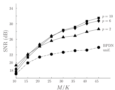
(a)

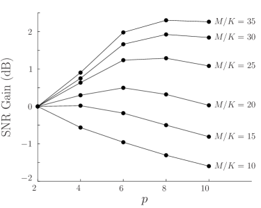
(b)

Figure 3: Reconstruction SNR of GBPDN$(\ell_{p,\boldsymbol{w}})$. (a): the dashed line represents the reconstruction quality achieved from uniformly quantized CS and BPDN. (b) SNR gain versus $p$ for each tested oversampling ratio $M/K$.

We observe that, given the oversampling ratio, these experimental results allow to increase $p$ to a greater extent than would be allowed by our theory deployed in Section IV. In particular, the sufficient condition (18) dictated by Proposition 1 requires the number of measurements $M$ to scale as $K^{p/2}$ (ignoring times the usual logarithmic terms) in order to ensure the RIP_p,w. This would imply an exponential increase in the number of measurements needed as $p$ increases. However, from Fig. 3(b), one can see that for $M/K=15$, $p=4$ was the largest value before performance starts degrading. With $M/K=20$, $p$ could be increased to 6 before degradation, and to 8 before degradation with $M/K=30$. At least for this example, we do not observe such a severe exponential dependence in the needed oversampling in order to benefit from error decrease when increasing $p$.

In Fig. 4, the quantization consistency of the reconstructed signals is tested by looking at the histogram of $\upalpha^{-1}(\mathcal{G}(\boldsymbol{\Phi}\boldsymbol{x}^{*})-\mathcal{G}(\boldsymbol{y}))$. We do observe that this histogram is closer to a uniform distribution for $p=10$ than for $p=2$, in good agreement with the “companded” quantizer definition $\mathcal{Q}=\mathcal{G}^{-1}\circ\mathcal{Q}_{\upalpha}\circ\mathcal{G}$ showing that in the domain compressed by $\mathcal{G}$, this quantizer is similar to a uniform one.

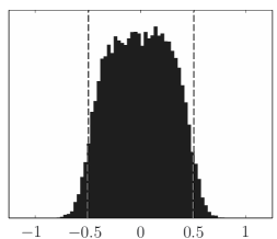
(a)

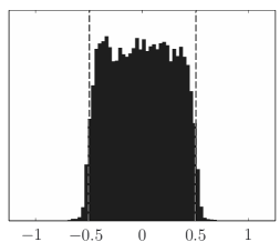
(b)

Figure 4: Testing the Quantization Consistency (QC). (a) Histogram of the components of $\upalpha^{-1}\,\big{(}\mathcal{G}(\boldsymbol{\Phi}\boldsymbol{x}^{*})-\mathcal{G}(\boldsymbol{y})\big{)}$ for $p=2$ and $M/K=40$ (averaged over 100 trials). (b) Same histogram for $p=10$. The QC is better respected in this case.

As a last test, we have more thoroughly compared a uniform quantization scenario described in the experimental setup above with the BPDQ_p decoder developed in [8] to the non-uniform case studied in this paper. More precisely, Fig. 5 shows the reconstruction SNR gain between non-uniform and uniform quantization at various $p$, i.e., SNR$($GBPDN$(\ell_{p,\boldsymbol{w}}))$ $-$ SNR$($BPDQ${}_{p})$. We see that, at a given $p$, this gain improves with $M/K$, and the highest SNR improvement values are obtained for $p=2$. This points the fact that for $p\neq 2$, the quantization scheme is not optimized for reducing the $\ell_{p,\boldsymbol{w}}$-norm distortion. This would require us to change the quantization scenario by not only optimizing the $p$-optimal levels but also the thresholds. This will be be left to a future research.

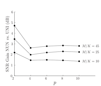
Figure 5: Reconstruction gain (in dB) between non-uniform or uniform quantization at the same $p$.

VI Conclusion

In this paper, we have shown that, when the compressive measurements of a sparse or compressible signal are non-uniformly quantized, there is a clear interest in modifying the reconstruction procedure by adapting the way it imposes the reconstructed signal to “match” the observed data. In particular, we have proved that in an oversampled scenario, replacing the common BPDN $\ell_{2}$-norm constraint by a weighted $\ell_{p}$-norm adjusted to the non-uniform nature of the quantizer reduces the reconstruction error by a factor of $\sqrt{p+1}$. Moreover, we showed that this improvement stems from a stabilization of the quantization distortion seen as an additive heteroscedastic GGD noise on the measurements.

In future work, we will investigate if the quantization scheme can also be optimized with respect to the proposed reconstruction procedure, i.e., by adjusting the thresholds for minimizing the weighted $\ell_{p}$-distortion at a fixed bit budget.

Appendix A Preparatory Lemmata

This appendix contains several key lemmata that are useful for the subsequent proofs developed in the other appendices.

The first lemma will serve later to evaluate asymptotically the contribution of each quantization bin to the global quantizer distortion measured with $\ell_{p,\boldsymbol{w}}$-norm when a Gaussian source (with pdf $\varphi_{0}$) is quantized.

Lemma 6.

Given $a,b\in\mathbb{R}$ with $a<b$, $n\in\mathbb{N}\setminus\{0\}$ and a Gaussian pdf $\varphi_{0}=\gamma_{0,\sigma_{0}}$. Let $\lambda_{n}$ be the (unique) minimizer of $\min_{\lambda\in[a,b]}\ \int_{a}^{b}|t-\lambda|^{n}\ \varphi_{0}(t)\,\mathrm{d}t$. Then,

$$\int_{a}^{b}|t-\lambda_{n}|^{n}\ \varphi_{0}(t)\,\mathrm{d}t\ \geqslant\ \tfrac{(b-a)^{n+1}}{(n+1)\,2^{n+1}}\,(1+(\tfrac{\mathsf{D}}{\mathsf{C}})^{-(n+1)/n})\,{\mathsf{C}},$$ (24)

$$\int_{a}^{b}|t-\lambda_{n}|^{n}\ \varphi_{0}(t)\,\mathrm{d}t\ \leqslant\ \tfrac{(b-a)^{n+1}}{(n+1)\,2^{n+1}}\,(1+(\tfrac{\mathsf{D}}{\mathsf{C}})^{(n+1)/n})\,{\mathsf{D}},$$ (25)

$$\tfrac{1}{1+\mathsf{S}^{1/n}}(\mathsf{S}^{1/n}a+b) \ \leqslant\ \lambda_{n}\ \leqslant\ \tfrac{1}{1+\mathsf{S}^{1/n}}(a+\mathsf{S}^{1/n}b),$$ (26)

with $\mathsf{C}:=\min_{t\in[a,b]}\varphi_{0}(t)$, $\mathsf{D}:=\max_{t\in[a,b]}\varphi_{0}(t)$ and $\mathsf{S}=\mathsf{D}/\mathsf{C}$.

Proof.

Let us first show the upper bound (25). In Lemma 1 and its proof, it was show that $\lambda_{n}$ exists and is unique, i.e., the minimization problem is well-posed. Furthermore, $\lambda_{n}$ satisfies

$$\mathsf{A}:=\int_{a}^{\lambda_{n}}(\lambda_{n}-t)^{n-1}\ \varphi_{0}(t)\,\mathrm{d}t\ =\ \int_{\lambda_{n}}^{b}(t-\lambda_{n})^{n-1}\ \varphi_{0}(t)\,\mathrm{d}t.$$

Since $\varphi_{0}(t)\in[\mathsf{C},\mathsf{D}]$ for $t\in[a,b]$, we have $(\lambda_{n}-a)^{n}\,\mathsf{C}\leqslant n\mathsf{A}\leqslant(\lambda_{n}-a)^{n}\,\mathsf{D}$ and $(b-\lambda_{n})^{n}\,\mathsf{C}\leqslant n\mathsf{A}\leqslant{\textstyle\frac{1}{n}}(b-\lambda_{n})^{n}\,\mathsf{D}$. This implies $(\lambda_{n}-a)^{n}\geqslant\big{(}\tfrac{\mathsf{C}}{\mathsf{D}}\big{)}(b-\lambda_{n})^{n}$ and $(b-\lambda_{n})^{n}\geqslant\big{(}\tfrac{\mathsf{C}}{\mathsf{D}}\big{)}(\lambda_{n}-a)^{n}$, from which we easily deduce (26).

Since $\int_{a}^{b}|t-\lambda_{n}|^{n}\ \varphi_{0}(t)\,\mathrm{d}t=\int_{a}^{\lambda_{n}}(\lambda_{n}-t)^{n}\ \varphi_{0}(t)\,\mathrm{d}t\ +\int_{\lambda_{n}}^{b}(t-\lambda_{n})^{n}\ \varphi_{0}(t)\,\mathrm{d}t$, we find $\int_{a}^{b}|t-\lambda_{n}|^{n}\ \varphi_{0}(t)\,\mathrm{d}t\leqslant{\textstyle\frac{1}{n+1}}\,[(\lambda_{n}-a)^{n+1}+(b-\lambda_{n})^{n+1}]\,\mathsf{D}$. From $((\lambda_{n}-a)/(b-\lambda_{n}))^{n}\in[\mathsf{C}/\mathsf{D},\mathsf{D}/\mathsf{C}]$, we find that $\int_{a}^{b}|t-\lambda_{n}|^{n}\ \varphi_{0}(t)\,\mathrm{d}t$ is smaller than

$${\textstyle\frac{1}{n+1}}\min\big{(}\,(\lambda_{n}-a)^{n+1},(b-\lambda_{n})^{n+1}\big{)}\left[1+\big{(}\tfrac{\mathsf{D}}{\mathsf{C}}\big{)}^{(n+1)/n}\right]\,\mathsf{D}.$$

This provides (25) since $\min(\lambda_{n}-a,b-\lambda_{n})\leqslant(b-a)/2$. The bound (24) is obtained similarly. ∎

The following lemma presents a generalization of “$Q$-function like” bounds for lower partial moments of a Gaussian pdf.

Lemma 7.

Let $\lambda>0$, $n\in\mathbb{N}$ and $\varphi=\gamma_{0,1}$. Let us define $Q_{n}(\lambda):=\int_{\lambda}^{+\infty}\ (t-\lambda)^{n}\varphi(t)\ \mathrm{d}t$. Then, $Q_{n}(\lambda)=\Theta(\lambda^{-(n+1)}\varphi(\lambda))$. More precisely, $\tfrac{n!\,\lambda^{n+1}}{\Pi_{k=1}^{n+1}(\lambda^{2}+k)}\,\varphi(\lambda)\ \leqslant\ Q_{n}(\lambda)\ \leqslant\ \tfrac{n!}{\lambda^{n+1}}\,\varphi(\lambda).$

This lemma generalizes the well known bound on $Q=Q_{0}$, namely $\tfrac{\lambda}{\lambda^{2}+1}\,\varphi(\lambda)\leqslant Q(\lambda)\leqslant\tfrac{1}{\lambda}\,\varphi(\lambda)$.

Proof.

The proof involves integration by parts, the identities $-\varphi^{\prime}(u)=u\varphi(u)$ and $({\varphi(u)}/{u^{n}})^{\prime}=(1+\tfrac{n}{u^{2}})\tfrac{\varphi(u)}{u^{n-1}}$. Therefore, the upper bound is a simple consequence of

$$Q_{n}(\lambda)\leqslant{\textstyle\frac{1}{\lambda}}\int_{\lambda}^{+\infty}(t-\lambda)^{n}\ t\varphi(t)\ \mathrm{d}t=\tfrac{n}{\lambda}\,Q_{n-1}(\lambda)\leqslant\cdots\leqslant\tfrac{n!}{\lambda^{n}}Q(\lambda)\leqslant\tfrac{n!}{\lambda^{n+1}}\varphi(\lambda).$$

To get the lower bound, observe first that, defining $Q_{n,k}(\lambda):=\int_{\lambda}^{+\infty}\ (t-\lambda)^{n}t^{-k}\varphi(t)\ \mathrm{d}t$, we find

$$(1+\tfrac{k+1}{\lambda^{2}})\,Q_{n,k}(\lambda)\geqslant\int_{\lambda}^{+\infty}\ (t-\lambda)^{n}(1+\tfrac{k+1}{t^{2}})\,t^{-k}\varphi(t)\ \mathrm{d}t=n\,Q_{n-1,k+1}(\lambda).$$

Therefore, $Q_{n}(\lambda)\geqslant\tfrac{n\lambda^{2}}{\lambda^{2}+1}\,Q_{n-1,1}(\lambda)\geqslant\cdots\geqslant\tfrac{n!\lambda^{2n}}{\Pi_{k=1}^{n}(\lambda^{2}+k)}\,Q_{0,n}(\lambda)$. But $(1+\tfrac{n+1}{\lambda^{2}})\,Q_{0,n}(\lambda)\geqslant{\varphi(\lambda)}/{\lambda^{n+1}}$, so that $Q_{n}(\lambda)\geqslant\tfrac{n!\lambda^{2n+2}}{\Pi_{k=1}^{n+1}(\lambda^{2}+k)}\,\tfrac{\varphi(\lambda)}{\lambda^{n+1}}$, which concludes the proof. ∎

Appendix B Proof of Lemma 1: “$p$-optimal Level Definiteness”

Proof.

For $2\leqslant p<\infty$, $|t-\lambda|^{p}$ is a continuous, coercive and strictly convex function of $\lambda$ over $\mathbb{R}$, and therefore so is $\int_{\mathcal{R}_{k}}|t-\lambda|^{p}\ \varphi_{0}(t)\,\mathrm{d}t$ since $\varphi_{0}(t)>0$. It follows that the function $\int_{\mathcal{R}_{k}}|t-\lambda|^{p}\ \varphi_{0}(t)\,\mathrm{d}t$ has a unique minimizer on $\mathbb{R}$. Moreover, this minimizer is necessarily located in $\mathcal{R}_{k}$ since $\int_{\mathcal{R}_{k}}|t-\lambda|^{p}\ \varphi_{0}(t)\,\mathrm{d}t$ is monotonically decreasing (resp. increasing) on $(-\infty,t_{k})$ (resp. $(t_{k+1},+\infty)$). Consequently, $\omega_{k,n}$ exists and is unique.

For proving the limit case $p\to\infty$, for finite bins $\mathcal{R}_{k}$ ($k\notin\{1,\mathcal{B}\}$) and without loss of generality for $t_{k}\geqslant 0$, relation (26) in Lemma 6 with $a=t_{k}$ and $b=t_{k+1}$, together with the squeeze theorem shows that

$$\lim_{p\to+\infty}\omega_{k,p}=\lim_{p\to+\infty}\tfrac{1}{1+\mathsf{S}^{1/p}}(\mathsf{S}^{1/p}t_{k}+t_{k+1})=\lim_{p\to+\infty}\tfrac{1}{1+\mathsf{S}^{1/p}}(t_{k}+\mathsf{S}^{1/p}t_{k+1})=\omega_{k,\infty}~{},$$

where $\mathsf{S}=\varphi_{0}(t_{k})/\varphi_{0}(t_{k+1})$.

For infinite bins (i.e., $k\in\{1,\mathcal{B}\}$) and assuming again $t_{k}\geqslant 0$, it follows from the beginning of the proof that $\omega_{k,p}$ is the unique root on $[t_{k},+\infty)$ of $\mathcal{E}_{p}(\lambda):=\int_{t_{k}}^{\lambda}(\lambda-t)^{p-1}\varphi_{0}(t)\,\mathrm{d}t-\int_{\lambda}^{\infty}(t-\lambda)^{p-1}\varphi_{0}(t)\,\mathrm{d}t$. Let $\tilde{\omega}_{k,p}\in[t_{k},L]$ be the root of $\tilde{\mathcal{E}}_{p}(\lambda,L):=\int_{t_{k}}^{\lambda}(\lambda-t)^{p-1}\varphi_{0}(t)\,\mathrm{d}t-\int_{\lambda}^{L}(t-\lambda)^{p-1}\varphi_{0}(t)\,\mathrm{d}t$ for some $L\geqslant t_{k}$. We then have $\mathcal{E}_{p}(\tilde{\omega}_{k,p})=\int_{t_{k}}^{\tilde{\omega}_{k,p}}({\tilde{\omega}_{k,p}}-t)^{p-1}\varphi_{0}(t)\,\mathrm{d}t-\int_{{\tilde{\omega}_{k,p}}}^{\infty}(t-{\tilde{\omega}_{k,p}})^{p-1}\varphi_{0}(t)\,\mathrm{d}t=-\int_{L}^{\infty}(t-{\tilde{\omega}_{k,p}})^{p-1}\varphi_{0}(t)\leqslant 0=\mathcal{E}_{p}(\omega_{k,p})$, which implies $\tilde{\omega}_{k,p}\leqslant\omega_{k,p}$ since $\mathcal{E}_{p}$ is non-decreasing for $p\geqslant 1$. However, since $\tilde{\omega}_{k,p}$ is optimal on $[t_{k},L]$, taking $L=L(p)=c\sqrt{p}$, for $c>0$, we have by Lemma 6 with $a=t_{k}$ and $b=L(p)$, $\lim_{p\to+\infty}\tilde{\omega}_{k,p}\geqslant\lim_{p\to+\infty}\tfrac{1}{1+\mathsf{S}^{1/p}}(\mathsf{S}^{1/p}t_{k}+c\sqrt{p})=+\infty$ since $\mathsf{S}^{1/p}=\exp(-t^{2}_{k}/2p\sigma_{0}^{2})\exp(c^{2}/2\sigma_{0}^{2})=\Theta(1)$. This proves $\lim_{p\to+\infty}|\omega_{k,p}|=+\infty=\omega_{k,\infty}$ and $|\omega_{k,p}|=\Omega(\sqrt{p})$ for $k\in\{1,\mathcal{B}\}$. ∎

Appendix C Proof of Lemma 2: “Asymptotic $p$-Quantization Characterization”

The content of Lemma 2 is derived from this larger set of results which constitutes a toolbox lemma for other developments given in these appendices.

Lemma 8 (Extended Asymptotic $p$-Quantization Characterization).

Given the Gaussian pdf $\varphi_{0}$ and its associated compressor $\mathcal{G}$ function, choose $0<\beta<1$ and $p\in\mathbb{N}$, and define $T=T(B)=\sqrt{6\,\sigma_{0}^{2}(\log 2^{\beta})\,B}$, $\mathcal{T}=[-T,T]$ and $\mathcal{T}^{c}=\mathbb{R}\setminus\mathcal{T}$. We have the following asymptotic properties (relative to $B$):

$$\mathcal{G}^{\prime}(T(B)) =\Theta(2^{-\beta B}),$$ (27)

$$\#\{k:\mathcal{R}_{k}\subset\mathcal{T}^{c}\} =\Theta\big{(}B^{-1/2}\,2^{(1-\beta)B}\big{)},$$ (28)

$$\int_{\mathcal{R}_{k}}|t-\omega_{k,p}|^{p}\ \varphi_{0}(t)\,\mathrm{d}t =O\big{(}B^{-(p+1)/2}\,2^{-3\beta B}\big{)},\quad\forall\mathcal{R}_{k}\subset\mathcal{T}^{c}.$$ (29)

Moreover, for all $k$ such that $\mathcal{R}_{k}\subset\mathcal{T}$ and any $c\in\mathcal{R}_{k}$

$$\uptau_{k}:=t_{k+1}-t_{k}=\ O(2^{-(1-\beta)B}),$$ (30)

$$1\ \leqslant\ \tfrac{\max(\varphi_{0}(t_{k}),\,\varphi_{0}(t_{k+1}))}{\min(\varphi_{0}(t_{k}),\,\varphi_{0}(t_{k+1}))}=\ \exp\big{(}O(B^{1/2}\,2^{-(1-\beta)B})\big{)}=1+O(B^{1/2}\,2^{-(1-\beta)B}),$$ (31)

$$\textstyle\int_{\mathcal{R}_{k}}|t-\omega_{k,p}|^{p}\ \varphi_{0}(t)\,\mathrm{d}t\ \simeq_{B}\ \tfrac{\uptau_{k}^{p+1}}{(p+1)\,2^{p}}\,\varphi_{0}(c),$$ (32)

$$\mathcal{G}^{\prime}(c)\simeq_{B}\tfrac{\upalpha}{\uptau_{k}}.$$ (33)

Finally, if $k$ is such that $T(B)\in\mathcal{R}_{k}$, then, writing the interval length/measure $\mathcal{L}(\mathcal{A})=\int_{\mathcal{A}}\mathrm{d}t$ for $\mathcal{A}\subset\mathbb{R}$,

$$\mathcal{L}(\mathcal{R}_{k}\cap\mathcal{T}) =\ O(2^{-(1-\beta)B}),$$ (34)

$$\mathcal{G}^{\prime}(\omega_{k,p}) \leqslant\max(\mathcal{G}^{\prime}(t_{k}),\mathcal{G}^{\prime}(t_{k+1}))=\ O(2^{-\beta B}),$$ (35)

$$\int_{\mathcal{R}_{k}}|t-\omega_{k,p}|^{p}\ \varphi_{0}(t)\,\mathrm{d}t\ =O\big{(}B^{-(p+1)/2}\,2^{-3\beta B}\big{)}.$$ (36)

Proof.

In this proof we use the quantizer symmetry to restrict the analysis to the half (positive) real line $\mathbb{R}_{+}$, on which $\varphi_{0}$ is decreasing.

Relation (27) comes from the definition of $T(B)$ and that of $\mathcal{G}^{\prime}=\gamma_{0,\sqrt{3}\,\sigma_{0}}$. For proving (28), we can observe that $\mathcal{G}(\lambda)=|\!|\!|\varphi_{0}|\!|\!|^{-1/3}_{1/3}\int_{-\infty}^{\lambda}\varphi_{0}^{1/3}(t)\,\mathrm{d}t=1-Q(\lambda/\sqrt{3}\sigma_{0})$ where $Q(t)={\textstyle\frac{1}{\sqrt{2\pi}}}\int_{t}^{+\infty}\gamma_{0,1}(u)\,\mathrm{d}u$. Since $\frac{\lambda}{1+\lambda^{2}}\gamma_{0,1}(\lambda)\leqslant Q(\lambda)\leqslant\tfrac{1}{\lambda}\gamma_{0,1}(\lambda)$, we obtain

$$\tfrac{3\sigma^{2}_{0}\lambda}{3\sigma_{0}^{2}+\lambda^{2}}\,\mathcal{G}^{\prime}(\lambda)\ \leqslant\ 1-\mathcal{G}(\lambda)\ \leqslant\ \tfrac{3\sigma_{0}^{2}}{\lambda}\,\mathcal{G}^{\prime}(\lambda).$$

Taking $\lambda=T(B)$ in the last inequalities and using (27), we deduce from the quantizer definition

$$\#\{k:\mathcal{R}_{k}\subset\mathcal{T}^{c}\}\ =\ 2\,\#\{k:t_{k}\geqslant T(B)\}\ =\ 2\,\upalpha^{-1}\,(1-\mathcal{G}(T))\ =\Theta\big{(}B^{-1/2}\,2^{(1-\beta)B}\big{)}.$$

Relation (29) is proved by noting that, if $t_{k}\geqslant T(B)$,

$$\int_{\mathcal{R}_{k}}|t-\omega_{k,p}|^{p}\ \varphi_{0}(t)\,\mathrm{d}t\leqslant\int_{\mathcal{R}_{k}}(t-t_{k})^{p}\ \varphi_{0}(t)\,\mathrm{d}t\leqslant\int_{t_{k}}^{\infty}(t-t_{k})^{p}\ \varphi_{0}(t)\,\mathrm{d}t,$$

where the first inequality follows from the $p$-optimality of $\omega_{k,p}\in\mathcal{R}_{k}$. However, from Lemma 7, we know that, for $\lambda\in\mathbb{R}_{+}$

$$\tfrac{p!\,\lambda^{p+1}\sigma_{0}^{2p+2}}{\Pi_{k=1}^{p+1}(\lambda^{2}+k\sigma_{0}^{2})}\,\varphi_{0}(\lambda)\ \leqslant\ \sigma_{0}^{p}\,Q_{p}(\tfrac{\lambda}{\sigma_{0}})\ \leqslant\ \tfrac{p!\,\sigma_{0}^{2p+2}}{\lambda^{p+1}}\,\varphi_{0}(\lambda),$$

with $Q_{p}(\lambda):=\int_{\lambda}^{\infty}\,(t-\lambda)^{p}\,\gamma_{0,1}(t)\ \mathrm{d}t$ and $\sigma_{0}^{p}\,Q_{p}(\tfrac{\lambda}{\sigma_{0}})=\int_{\lambda}^{\infty}\,(t-\lambda)^{p}\,\varphi_{0}(t)\ \mathrm{d}t$.

Therefore, since $\varphi_{0}\propto(\mathcal{G}^{\prime})^{3}$,

$$\int_{t_{k}}^{\infty}(t-t_{k})^{p}\ \varphi_{0}(t)\,\mathrm{d}t\leqslant\ \tfrac{p!\,\sigma_{0}^{2(p+1)}}{t_{k}^{p+1}}\,\varphi_{0}(t_{k})\leqslant\tfrac{p!\,\sigma_{0}^{2(p+1)}}{T^{p+1}}\,\varphi_{0}(T)=O\big{(}B^{-(p+1)/2}\,2^{-3\beta B}\big{)}.$$

Relation (30) is obtained by observing that $\mathcal{G}$ is concave on $\mathbb{R}_{+}$. This implies $\uptau_{k}\leqslant\upalpha/\mathcal{G}^{\prime}(t_{k+1})$ and if $k$ is such that $0\leqslant t_{k+1}\leqslant T(B)$, $\uptau_{k}=O(2^{-(1-\beta)B})$. For (31), keeping the same $k$, we note that $1\leqslant\frac{\varphi_{0}(t_{k})}{\varphi_{0}(t_{k+1})}=\exp(\frac{1}{6\sigma_{0}^{2}}\uptau_{k}(t_{k}+t_{k+1}))\leqslant\exp(\frac{1}{3\sigma_{0}^{2}}\uptau_{k}t_{k+1})=\exp\big{(}O(B^{1/2}\,2^{-(1-\beta)B})\big{)}$ which is then arbitrarily close to 1.

For proving (32), we assume first $p\geqslant 1$. Let us consider (24) and (25) with $a=t_{k}$, $b=t_{k+1}$, $\mathsf{C}=\varphi_{0}(t_{k+1})$ and $\mathsf{D}=\varphi_{0}(t_{k})$ with $0\leqslant t_{k+1}\leqslant T(B)$. From (31) we see that $1\leqslant\tfrac{\mathsf{D}}{\mathsf{C}}=1+o(1)$. We show easily that this involves the equivalent relations $\mathsf{C}\simeq_{B}\mathsf{D}$, $\mathsf{C}/\mathsf{D}\simeq_{B}1$ and $\mathsf{D}/\mathsf{C}\simeq_{B}1$. Therefore, $(1+(\mathsf{D}/\mathsf{C})^{(p+1)/p})\simeq_{B}2$ and $(1+(\mathsf{C}/\mathsf{D})^{(p+1)/p})\simeq_{B}2$. Moreover, $\mathsf{C}\simeq_{B}\varphi_{0}(c)$ and $\mathsf{D}\simeq_{B}\varphi_{0}(c)$ for any $c\in\mathcal{R}_{k}$, so that (24) and (25)) show finally $\int_{\mathcal{R}_{k}}|t-\omega_{k,p}|^{p}\ \varphi_{0}(t)\,\mathrm{d}t\ \mathop{\lesssim}_{B}\ \tfrac{\uptau_{k}^{p+1}}{(p+1)\,2^{p}}\,\varphi_{0}(c)$ and $\int_{\mathcal{R}_{k}}|t-\omega_{k,p}|^{p}\ \varphi_{0}(t)\,\mathrm{d}t\ \mathop{\gtrsim}_{B}\ \tfrac{\uptau_{k}^{p+1}}{(p+1)\,2^{p}}\,\varphi_{0}(c)$, which proves the relation. The case $p=0$ is demonstrated similarly by observing that $\varphi_{0}(t_{k+1})\uptau_{k}\leqslant p_{k}:=\int_{\mathcal{R}_{k}}\varphi_{0}(t)\,\mathrm{d}t\leqslant\varphi_{0}(t_{k})\uptau_{k}$.

Let’s now turn to showing (33). From (31) and since $\mathcal{G}^{\prime}\propto\varphi_{0}^{1/3}$, $1\leqslant\mathcal{G}^{\prime}(t_{k})/\mathcal{G}^{\prime}(t_{k+1})=1+o(1)$ so that $\mathcal{G}^{\prime}(t_{k})/\mathcal{G}^{\prime}(t_{k+1})\simeq_{B}1$. By concavity of $\mathcal{G}$ on $\mathbb{R}_{+}$, we know that $\mathcal{G}^{\prime}(t_{k+1})\leqslant\upalpha/\uptau_{k}\leqslant\mathcal{G}^{\prime}(t_{k})$. Therefore, $1\leqslant(\mathcal{G}^{\prime}(t_{k+1}))^{-1}\upalpha/\uptau_{k}=1+o(1)$ which yields $\mathcal{G}^{\prime}(t_{k+1})\simeq_{B}\upalpha/\uptau_{k}$. By the concavity argument again, we have $\mathcal{G}^{\prime}(t_{k})\geqslant\mathcal{G}^{\prime}(c)\geqslant\mathcal{G}^{\prime}(t_{k+1})$ for any $c\in\mathcal{R}_{k}$, and thus $1+o(1)=\mathcal{G}^{\prime}(t_{k})/\mathcal{G}^{\prime}(t_{k+1})\geqslant\mathcal{G}^{\prime}(c)/\mathcal{G}^{\prime}(t_{k+1})\geqslant 1$. This implies $\mathcal{G}^{\prime}(c)\simeq_{B}\mathcal{G}^{\prime}(t_{k+1})\simeq_{B}\upalpha/\uptau_{k}$.

If $k$ is such that $0\leqslant t_{k}\leqslant T(B)\leqslant t_{k+1}$, using again the concavity of $\mathcal{G}$ on $\mathbb{R}_{+}$, we find $\mathcal{L}(\mathcal{R}_{k}\cap\mathcal{T})=T(B)-t_{k}\leqslant\mathcal{(}\mathcal{G}(T(B))-k\upalpha)/\mathcal{G}^{\prime}(T(B))\leqslant\upalpha/\mathcal{G}^{\prime}(T(B))=O(2^{-(1-\beta)B})$, which proves (34).

For showing (35), we note that $\mathcal{G}^{\prime}(t_{k})=\mathcal{G}^{\prime}(T)(\mathcal{G}^{\prime}(t_{k})/\mathcal{G}^{\prime}(T))$. Since $\mathcal{G}^{\prime}(t_{k})/\mathcal{G}^{\prime}(T)=\exp(\frac{1}{6\sigma_{0}^{2}}(T-t_{k})(T+t_{k}))\leqslant\exp(\frac{1}{3\sigma_{0}^{2}}(T-t_{k})T)=\exp(O(B^{1/2}\,2^{-(1-\beta)B}))$ which is arbitrarily close to 1 (i.e., it is $e^{o(1)}$), we find $\mathcal{G}^{\prime}(t_{k})=O(2^{-\beta B})$, i.e., it inherits the behavior of $\mathcal{G}^{\prime}(T)$.

The last relation (36) is proved similarly to (29) by appealing again to Lemma 7,

$$\int_{\mathcal{R}_{k}}(t-t_{k})^{p}\ \varphi_{0}(t)\,\mathrm{d}t\ \leqslant\ \int_{t_{k}}^{\infty}(t-t_{k})^{p}\ \varphi_{0}(t)\,\mathrm{d}t\leqslant\ \tfrac{p!\,\sigma_{0}^{2p+2}}{t_{k}^{p+1}}\,\varphi_{0}(t_{k})=O\big{(}B^{-(p+1)/2}\,2^{-3\beta B}\big{)},$$

where the asymptotic relation is obtained by seeing that, as soon as $T-t_{k}\leqslant 1/2$ (which is always possible to meet thanks to (34)),

$$\tfrac{1}{t_{k}}=\tfrac{1}{T}(1-\tfrac{T-t_{k}}{T})^{-1}\leqslant\tfrac{1}{T}\,(1+2\tfrac{T-t_{k}}{T}),$$

and $\varphi_{0}(t_{k})=O(2^{-3\beta B})$ since $\varphi_{0}\propto(\mathcal{G}^{\prime})^{3}$. ∎

Appendix D Proof of Lemma 3: “Asymptotic Weighted $\ell_{p}$-Distortion”

Before proving Lemma 3, let us show the following asymptotic equivalence.

Lemma 9.

Let $p\in\mathbb{N}\setminus\{0\}$ and $\gamma>p-3$.

$$\sum_{k=1}^{\mathcal{B}}\ [\mathcal{G}^{\prime}(\omega_{k,p})]^{\gamma}\int_{\mathcal{R}_{k}}|t-\omega_{k,p}|^{p}\,\varphi_{0}(t)\,\mathrm{d}t\ \simeq_{B}\ \tfrac{2^{-pB}}{(p+1)\,2^{p}}\,\int_{\mathbb{R}}[\mathcal{G}^{\prime}(t)]^{\gamma-p}\varphi_{0}(t)\,\mathrm{d}t,$$ (37)

Proof.

Let us use the threshold $T(B)$ defined in Lemma 8 for splitting the sum (37) in two parts, i.e., using the quantizer symmetry,

$$\sum_{k=1}^{\mathcal{B}}\ [\mathcal{G}^{\prime}(\omega_{k,p})]^{\gamma}\int_{\mathcal{R}_{k}}|t-\omega_{k,p}|^{p}\,\varphi_{0}(t)\,\mathrm{d}t=\ 2\!\!\!\!\!\!\sum_{k:\ 0\leqslant t_{k+1}<T(B)}\ [\mathcal{G}^{\prime}(\omega_{k,p})]^{\gamma}\int_{\mathcal{R}_{k}}|t-\omega_{k,p}|^{p}\,\varphi_{0}(t)\,\mathrm{d}t\quad+\quad\mathsf{R},$$

where the residual $\mathsf{R}$ reads

$$\mathsf{R} :=\ 2\!\!\!\!\!\!\sum_{k:\ t_{k+1}\geqslant\,T(B)}\ [\mathcal{G}^{\prime}(\omega_{k,p})]^{\gamma}\int_{\mathcal{R}_{k}}|t-\omega_{k,p}|^{p}\,\varphi_{0}(t)\,\mathrm{d}t,$$

$$\,=\ 2\,[\mathcal{G}^{\prime}(\omega_{k^{\prime},p})]^{\gamma}\int_{\mathcal{R}_{k^{\prime}}}|t-\omega_{k^{\prime},p}|^{p}\,\varphi_{0}(t)\,\mathrm{d}t\ +\ 2\!\!\!\!\sum_{k:\ t_{k}\geqslant\,T(B)}\ [\mathcal{G}^{\prime}(\omega_{k,p})]^{\gamma}\int_{\mathcal{R}_{k}}|t-\omega_{k,p}|^{p}\,\varphi_{0}(t)\,\mathrm{d}t,$$

where $k^{\prime}$ is such that $t_{k^{\prime}}<T(B)\leqslant t_{k^{\prime}+1}$.

From Lemma 8, we can easily bound this residual. We know from (27), (29), (35) and (36) that, for all $k\in\ \{j:\omega_{j,p}\geqslant t_{j}\geqslant T(B)\}\cup\{k^{\prime}\}$,

$$\ [\mathcal{G}^{\prime}(\omega_{k,p})]^{\gamma}\int_{\mathcal{R}_{k}}|t-\omega_{k,p}|^{p}\,\varphi_{0}(t)\,\mathrm{d}t=O(2^{-\beta(\gamma+3)B}B^{-(p+1)/2}).$$

However, (28) tells us that the sum in $\mathsf{R}$ is made of no more than $1+O\big{(}B^{-1/2}\,2^{(1-\beta)B}\big{)}=O\big{(}B^{-1/2}\,2^{(1-\beta)B}\big{)}$ terms, so that

$$\mathsf{R}=O\big{(}B^{-(p+2)/2}\,2^{-(\beta(\gamma+4)-1)B}\big{)}.$$

Let us now study the terms for which $0\leqslant t_{k+1}\leqslant T(B)$. Using (32) and (33) provides

$$\sum_{k=1}^{\mathcal{B}}\ [\mathcal{G}^{\prime}(\omega_{k,p})]^{\gamma}\int_{\mathcal{R}_{k}}|t-\omega_{k,p}|^{p}\,\varphi_{0}(t)\,\mathrm{d}t$$

$$\mathop{\simeq}_{B}\ 2\,\sum_{k:\,0\leqslant t_{k+1}\leqslant T(B)}\ [\mathcal{G}^{\prime}(\omega_{k,p})]^{\gamma}\tfrac{\uptau_{k}^{p+1}}{(p+1)\,2^{p}}\,\varphi_{0}(\omega_{k,p})\ +\ \mathsf{R}$$

$$\mathop{\simeq}_{B}\ 2\tfrac{\upalpha^{p}}{(p+1)\,2^{p}}\,\sum_{k:\,0\leqslant t_{k+1}\leqslant T(B)}\ [\mathcal{G}^{\prime}(\omega_{k,p})]^{\gamma-p}\,\varphi_{0}(\omega_{k,p})\,\uptau_{k}\ +\ \mathsf{R}$$

$$\mathop{\simeq}_{B}\ 2\tfrac{2^{-pB}}{(p+1)\,2^{p}}\,\int_{0}^{T(B)}[\mathcal{G}^{\prime}(t)]^{\gamma-p}\varphi_{0}(t)\,\mathrm{d}t\ +\ \mathsf{R},$$

where, knowing that $0\leqslant t_{k+1}\leqslant T(B)$, we have also used (32) with $p=0$ to see that $p_{k}=\int_{\mathcal{R}_{k}}\varphi_{0}(t)\,\mathrm{d}t\simeq_{B}\varphi_{0}(c^{\prime})\uptau_{k}$ for any $c^{\prime}\in\mathcal{R}_{k}$.

Therefore, provided that $\beta(\gamma+4)\geqslant p+1$, which means that $\gamma>p-3$ since $\beta<1$, the residual $\mathsf{R}$ decreases faster than the first term in the right-hand side of last of the last equivalence relation, so that

$$\sum_{k=1}^{\mathcal{B}}\ [\mathcal{G}^{\prime}(\omega_{k,p})]^{\gamma}\int_{\mathcal{R}_{k}}|t-\omega_{k,p}|^{p}\,\varphi_{0}(t)\,\mathrm{d}t\ \mathop{\simeq}_{B}\ \tfrac{2^{-pB}}{(p+1)\,2^{p}}\,\int_{\mathbb{R}}[\mathcal{G}^{\prime}(t)]^{\gamma-p}\varphi_{0}(t)\,\mathrm{d}t,$$

since $T(B)=\Theta(B^{1/2})$ by definition. ∎

With the three previous lemmata under our belts, we are now ready to prove Lemma 3.

Proof of Lemma 3.

For $z_{i}\sim_{\operatorname{iid}}\mathcal{N}(0,\sigma_{0}^{2})$ with pdf $\varphi_{0}$, using the SLLN applied to $z_{i}$ conditionally on each quantization bin, we have

$$\|\mathcal{Q}_{p}[\boldsymbol{z}]-\boldsymbol{z}\|^{p}_{p,\boldsymbol{w}} :=\ \sum_{i=1}^{M}\ [\mathcal{G}^{\prime}(\mathcal{Q}_{p}[z_{i}])]^{p-2}\,|z_{i}-\mathcal{Q}_{p}[z_{i}]|^{p},$$

$$\mathop{\simeq}_{M}\ M\,\sum_{k=1}^{\mathcal{B}}\ [\mathcal{G}^{\prime}(\omega_{k,p})]^{p-2}\int_{\mathcal{R}_{k}}|t-\omega_{k,p}|^{p}\,\varphi_{0}(t)\,\mathrm{d}t,$$

where we used implicitly the quantizer symmetry in the last relation. This last relation is characterized by Lemma 9 by taking $n=p$ and $\gamma=p-2>p-3$, so that

$$\|\mathcal{Q}_{p}[\boldsymbol{z}]-\boldsymbol{z}\|^{p}_{p,\boldsymbol{w}} \mathop{\simeq}_{M,B}\ M\,\tfrac{2^{-pB}}{(p+1)\,2^{p}}\,\int_{\mathbb{R}}[\mathcal{G}^{\prime}(t)]^{-2}\varphi_{0}(t)\,\mathrm{d}t,$$

$$\mathop{\simeq}_{M,B}\ M\,\tfrac{2^{-pB}}{(p+1)2^{p}}\,|\!|\!|\varphi_{0}|\!|\!|_{1/3}.$$

∎

Appendix E Proof of Lemma 5: “Gaussian $\ell_{p,w}$-Norm Expectation”

First, the inequality ${\mathbb{E}}\|\boldsymbol{\xi}\|_{p,\boldsymbol{w}}\leqslant({\mathbb{E}}\|\boldsymbol{\xi}\|^{p}_{p,\boldsymbol{w}})^{1/p}$ follows from the Jensen inequality applied on the convex function $(\cdot)^{p}$ on $\mathbb{R}_{+}$. Second, from our result in [8, Appendix C] it is easy to show that

$${\mathbb{E}}\|\boldsymbol{\xi}\|_{p,\boldsymbol{w}}\geqslant({\mathbb{E}}\|\boldsymbol{\xi}\|^{p}_{p,\boldsymbol{w}})^{1/p}\,\big{(}1\ +\ ({\mathbb{E}}\|\boldsymbol{\xi}\|^{p}_{p,\boldsymbol{w}})^{-2}\operatorname{Var}\|\boldsymbol{\xi}\|^{p}_{p,\boldsymbol{w}}\big{)}^{\frac{1}{p}-1}.$$

Moreover, ${\mathbb{E}}\|\boldsymbol{\xi}\|^{p}_{p,\boldsymbol{w}}=\|\boldsymbol{w}\|_{p}^{p}\,{\mathbb{E}}|\mathcal{Z}|^{p}$, while

$$\operatorname{Var}\|\boldsymbol{\xi}\|^{p}_{p,\boldsymbol{w}}\ =\ \sum_{i}\operatorname{Var}|w_{i}\mathcal{Z}|^{p}=\|\boldsymbol{w}\|_{2p}^{2p}\operatorname{Var}|\mathcal{Z}|^{p}.$$

Therefore, assuming CM weights,

$${\mathbb{E}}\|\boldsymbol{\xi}\|_{p,\boldsymbol{w}}/({\mathbb{E}}\|\boldsymbol{\xi}\|^{p}_{p,\boldsymbol{w}})^{1/p} \geqslant\ \big{(}1\ +\ (\rho^{\max}_{2p}/\rho^{\min}_{p})^{2p}M^{-1}({\mathbb{E}}|\mathcal{Z}|^{p})^{-2}\operatorname{Var}|\mathcal{Z}|^{p}\big{)}^{\frac{1}{p}-1}$$

$$\geqslant\ \big{(}1\ +\ 2^{p+1}\,\theta_{p}^{p}\,M^{-1}\big{)}^{\frac{1}{p}-1},$$

since $\rho_{2p}^{\max}\leqslant\rho_{\infty}^{\max}$, and $({\mathbb{E}}|\mathcal{Z}|^{p})^{-2}\operatorname{Var}|\mathcal{Z}|^{2p}<2^{p+1}$ [8].

Appendix F Proof of Proposition 1: “RIP_p,w Matrix Existence”

The proof proceeds simply by considering the Lipschitz function $F(\boldsymbol{u})=\|\boldsymbol{u}\|_{p,\boldsymbol{w}}$ and the expected value $\mu=F(\boldsymbol{\xi})$ for a random vector $\boldsymbol{\xi}\sim\mathcal{N}^{M}(0,1)$ in [8, Appendix A]. The Lipschitz constant of $F$ is

$$\lim_{\boldsymbol{u}{\mathop{\to}_{\neq}}\boldsymbol{v}}\big{|}F(\boldsymbol{u})-F(\boldsymbol{v})\big{|}\,/\,\|\boldsymbol{u}-\boldsymbol{v}\|\ =\ \|\boldsymbol{w}\|_{\infty}\,\lambda_{p},$$

with $\lambda_{p}=\max(M^{(2-p)/2p},1)$ for $p\geqslant 1$. The value $\mu={\mathbb{E}}\|\boldsymbol{\xi}\|_{p,\boldsymbol{w}}$ can be estimated thanks to Lemma 5. Indeed, it tells us that if $M\geqslant 2(2\theta_{p})^{p}$,

$$\mu\ \geqslant\ {\textstyle\frac{1}{2}}({\mathbb{E}}\|\boldsymbol{\xi}\|^{p}_{p,\boldsymbol{w}})^{1/p}\geqslant\ {\textstyle\frac{1}{2}}\,\rho^{\min}_{p}\nu_{p}\,M^{1/p},$$

with $\nu_{p}^{p}={\mathbb{E}}|\mathcal{Z}|^{p}=2^{p/2}\pi^{-1/2}\Gamma(\tfrac{p+1}{2})$.

Inserting these results in [8, Appendix A], it is easy to show that a matrix $\boldsymbol{\Phi}\sim\mathcal{N}^{M\times N}(0,1)$ is RIP${}_{p,\boldsymbol{w}}(K,\delta,\mu)$ with a probability higher than $1-\eta$ if

$$M^{2/\!\max(2,p)}\ \geqslant\ c\,\big{(}\tfrac{\rho^{\max}_{\infty}}{\delta\,\rho_{p}^{\min}}\big{)}^{2}\big{(}K\log[e\tfrac{N}{K}(1+12\delta^{-1})]\ +\ \log\tfrac{2}{\eta}\big{)},$$

for some constant $c>0$.

Appendix G Proof of Proposition 3: Dequantizing Reconstruction Error

Proof.

We have to bound $\epsilon_{p}/{\mathbb{E}}\|\boldsymbol{\xi}\|_{p,\boldsymbol{w}}$, with $\boldsymbol{\xi}\sim\mathcal{N}^{M}(0,1)$, when $M$ is large and under the HRA. First, according to Lemma 5, using the SLLN and using the same decomposition than in the proof of Lemma 3 with the threshold $T(B)$ (with $\beta=(p+1)/(p+2)$) and the bounds provided by Lemma 8, we find almost surely

$$\mu^{p}\ :=\ ({\mathbb{E}}\|\boldsymbol{\xi}\|_{p,\boldsymbol{w}})^{p}\ \mathop{\simeq}_{M}\ \sum_{i=1}^{M}\,[\mathcal{G}^{\prime}(\mathcal{Q}_{p}[z_{i}])]^{p-2}{\mathbb{E}}|\mathcal{Z}|^{p}$$

$$\mathop{\simeq}_{M}\ M\,{\mathbb{E}}|\mathcal{Z}|^{p}\,\sum_{k:\,t_{k}\geqslant 0}p_{k}\,[\mathcal{G}^{\prime}(\omega_{k,p})]^{p-2}.$$

The sum in the last expression is characterized by Lemma 9 by setting inside (37) $n=0$ and $\gamma=p-2$. This provides

$$\mu^{p}\ \mathop{\simeq}_{M,B}\ M\,{\mathbb{E}}|\mathcal{Z}|^{p}\,\int_{\mathbb{R}}[\mathcal{G}^{\prime}(t)]^{p-2}\varphi_{0}(t)\,\mathrm{d}t$$

$$\mathop{\simeq}_{M,B}\ M\,{\mathbb{E}}|\mathcal{Z}|^{p}\,\big{[}\int_{\mathbb{R}}\varphi_{0}^{1/3}(t)\big{]}^{2-p}\,\big{[}\int_{\mathbb{R}}\varphi_{0}^{(p+1)/3}(t)\,\mathrm{d}t\big{]}.$$

Therefore, using the value $\epsilon_{p}$ defined in Lemma 3,

$$\tfrac{\epsilon^{p}}{\mu^{p}}\mathop{\simeq}_{B,M}\tfrac{2^{-p(B+1)}}{(p+1)\,{\mathbb{E}}|\mathcal{Z}|^{p}}\,|\!|\!|\varphi_{0}|\!|\!|^{(p+1)/3}_{1/3}\,|\!|\!|\varphi_{0}|\!|\!|^{-(p+1)/3}_{(p+1)/3}$$

However, for $\alpha>0$,

$$|\!|\!|\varphi_{0}|\!|\!|^{\alpha}_{\alpha}:=\int_{\mathbb{R}}\varphi^{\alpha}_{0}(t)\,\mathrm{d}t=(2\pi\sigma_{0}^{2})^{-\alpha/2}\,(2\pi\sigma_{0}^{2}/\alpha)^{1/2}\ \int_{\mathbb{R}}\gamma_{0,\sigma_{0}/\sqrt{\alpha}}(t)\,\mathrm{d}t\ =\ (2\pi\sigma_{0}^{2})^{(1-\alpha)/2}/\sqrt{\alpha}.$$

Consequently, $|\!|\!|\varphi_{0}|\!|\!|^{(p+1)/3}_{1/3}=3^{(p+1)/2}\,(2\pi\sigma_{0}^{2})^{(p+1)/3}$ and $|\!|\!|\varphi_{0}|\!|\!|^{(p+1)/3}_{(p+1)/3}=(2\pi\sigma_{0}^{2})^{(2-p)/6}/\sqrt{(p+1)/3}$, so that

$$\tfrac{\epsilon^{p}}{\mu^{p}}\mathop{\simeq}_{B,M}\tfrac{2^{-p(B+1)}}{\sqrt{p+1}\,{\mathbb{E}}|\mathcal{Z}|^{p}}\,(6\pi\sigma_{0}^{2})^{p/2}$$

Knowing that $({\mathbb{E}}|\mathcal{Z}|^{p})^{1/p}\geqslant c\,\sqrt{p+1}$ with $c=8\sqrt{2}/(9\sqrt{e})$ [8], we get

$$\tfrac{\epsilon}{\mu}\ \lesssim_{B,M}\ c^{\prime}\,2^{-B}\,\,\tfrac{(p+1)^{-\frac{1}{2p}}}{\sqrt{p+1}}\leqslant c^{\prime}\,\frac{2^{-B}}{\sqrt{p+1}}.$$

with $c^{\prime}=(9/8)(e\pi/3)^{1/2}$. ∎

Appendix H Computation of the $\omega_{k,p}$

This section describes a numerical procedure for efficiently computing the $p$-optimal levels $\omega_{k,p}$ of a Gaussian source $\mathcal{N}(0,1)$ for integer $p\geqslant 2$, defined by $\omega_{k,p}:=\operatorname*{argmin}_{\lambda\in\mathcal{R}_{k}}\mathcal{E}_{k,p}(\lambda)$, where $\mathcal{E}_{k,p}(\lambda)=\int_{t_{k}}^{t_{k+1}}|t-\lambda|^{p}\ \gamma_{0,1}(t)\,\mathrm{d}t.$ As $\mathcal{E}_{k,p}(\lambda)$ is strictly convex and differentiable, the desired $\omega_{k,p}$ are the unique stationary points satisfying $\mathcal{E}^{\prime}_{k,p}(\omega_{k,p})=0$.

We compute the $\omega_{k,p}$ by Newton method, using standard numerical quadrature for $\mathcal{E}^{\prime}_{k,p}$ and $\mathcal{E}^{\prime\prime}_{k,p}$. We handle the semi-infinite bins by replacing $t_{1}=-\infty$ and $t_{\mathcal{B}}=\infty$ by -39 and +39, respectively (chosen as the smallest integer $x$ so that $\gamma_{0,1}(x)=0$ when evaluated in double precision floating point arithmetic). Given quadrature weights $c_{i}$, we approximate $\mathcal{E}_{k,p}$ by $\tilde{\mathcal{E}}_{k,p}(\lambda)=\sum_{i=1}^{N}c_{i}\gamma_{0,1}(x_{i})|x_{i}-\lambda|^{p}$ with $x_{i}=t_{k}+(i-1)\Delta x$, where $\Delta x=(t_{k+1}-t_{k})/(N-1)$. We then have $\tilde{\mathcal{E}^{\prime}}_{k,p}(\lambda)=\sum_{i=1}^{N}c_{i}\gamma_{0,1}(x_{i})p|x_{i}-\lambda|^{p-1}{\rm sign}\,(x_{i}-\lambda)$ and $\tilde{\mathcal{E}^{\prime\prime}}_{k,p}(\lambda)=\sum_{i=1}^{N}c_{i}\gamma_{0,1}(x_{i})p(p-1)|x_{i}-\lambda|^{p-2}$. We initialize with the midpoint for each of the finite bins, i.e., set $\lambda_{k}^{(0)}=(t_{k}+t_{k+1})/2$ for $2\leqslant k\leqslant\mathcal{B}-1$, and $\lambda_{1}^{(0)}=t_{2}$, $\lambda_{\mathcal{B}}^{(0)}=t_{\mathcal{B}-1}$ for the semi-infinite bins. For each $k$ we then iterate the Newton step $\lambda_{k}^{(n)}=\lambda_{k}^{(n-1)}-\tilde{\mathcal{E}^{\prime}}_{k,p}(\lambda_{k}^{(n-1)})/\tilde{\mathcal{E}}^{\prime\prime}_{k,p}(\lambda_{k}^{(n-1)})$ until the convergence criterion $|(\lambda_{k}^{n}-\lambda_{k}^{n-1})/\lambda_{k}^{n}|<10^{-15}$ is met. We used $c_{i}$ given by the fourth-order accurate Simpson’s rule, e.g., $\boldsymbol{c}=(1,4,2,4\ldots 2,4,1)\Delta x/3$, which yielded empirically observed $O(N^{-4})$ convergence of the calculated $w_{k,p}$. Results in this paper employed $N=10^{4}+1$ quadrature points, sufficient to yield $w_{k,p}$ accurate to machine precision.

References

- [1] D. L. Donoho, “Compressed Sensing,” IEEE Trans. Inf. Theory, vol. 52, no. 4, pp. 1289–1306, 2006.
- [2] E. J. Candès, “The restricted isometry property and its implications for compressed sensing,” Compte Rendus Acad. Sc., Paris, Serie I, vol. 346, pp. 589–592, 2008.
- [3] W. Dai, H. V. Pham, and O. Milenkovic, “Information theoretical and algorithmic approaches to quantized compressive sensing,” IEEE Trans. Comm., vol. 59, no. 7, pp. 1857–1866, 2011.
- [4] J. Laska, P. Boufounos, M. Davenport, and R. Baraniuk, “Democracy in action: Quantization, saturation, and compressive sensing,” App. Comp. and Harm. Anal., vol. 31, no. 3, pp. 429–443, November 2011.
- [5] A. Zymnis, S. Boyd, and E. Candès, “Compressed sensing with quantized measurements,” IEEE Sig. Proc. Letters, vol. 17, no. 2, pp. 149–152, Feb. 2010.
- [6] L. Jacques, J. N. Laska, P. T. Boufounos, and R. G. Baraniuk, “Robust 1-Bit Compressive Sensing via Binary Stable Embeddings of Sparse Vectors,” IEEE Trans. Inf. Theory, vol. 59, no. 4, pp. 2082-2102, Apr. 2013.
- [7] Y. Plan and R. Vershynin, “One-bit compressed sensing by linear programming,” Comm. Pure App. Math., Feb. 2013.
- [8] L. Jacques, D. K. Hammond, and M. J. Fadili, “Dequantizing Compressed Sensing: When Oversampling and Non-Gaussian Constraints Combine.,” IEEE Trans. Inf. Theory, vol. 57, no. 1, pp. 559–571, Jan. 2011.
- [9] R. M. Gray and D. L. Neuhoff, “Quantization,” IEEE Trans. Inf. Theory, vol. 44, no. 6, pp. 2325–2383, 1998.
- [10] N. T. Thao and M. Vetterli, “Reduction of the MSE in R-times oversampled A/D conversion to ”. IEEE Trans. Sig. Proc., vol. 42, no. 1, pp. 200-203, 1994.
- [11] V. K. Goyal, M. Vetterli, N. T. Thao, “Quantized Overcomplete Expansions in : Analysis, Synthesis, and Algorithms”, IEEE Trans. Inf. Theory, vol. 44, no. 1, pp. 16–31, 1998.
- [12] U. Kamilov, V.K. Goyal, and S. Rangan, “Optimal quantization for compressive sensing under message passing reconstruction,” in IEEE Int. Symp. Inf. Theory Proc. (ISIT), 2011, pp. 459–463.
- [13] S. Güntürk, A. Powell, R. Saab, and Ö. Yılmaz, “Sobolev duals for random frames and sigma-delta quantization of compressed sensing measurements,” Found. Comp. Math., vol. 13, no. 1, pp. 1–36, 2013.
- [14] D. E. Knuth, “Big omicron and big omega and big theta,” ACM Sigact News, vol. 8, no. 2, pp. 18–24, 1976.
- [15] J. N. Laska, P. Boufounos, and R. G. Baraniuk, “Finite-range scalar quantization for compressive sensing,” in Conf. Sampling Th. Appl. (SampTA), 2009.
- [16] S. Lloyd, “Least squares quantization in PCM,” IEEE Trans. Inf. Theory, vol. 28, no. 2, pp. 129–137, Mar. 1982.
- [17] J. Max, “Quantizing for minimum distortion,” IEEE Trans. Inf. Theory, vol. 6, no. 1, pp. 7–12, Mar. 1960.
- [18] P. F. Panter and W. Dite, “Quantization distortion in pulse-count modulation with nonuniform spacing of levels,” Proc. IRE, vol. 39, no. 1, pp. 44–48, 1951.
- [19] S. S. Chen, D. L. Donoho, and M. A. Saunders, “Atomic Decomposition by Basis Pursuit,” SIAM J. Sc. Comp., vol. 20, no. 1, pp. 33–61, 1998.
- [20] J.-J. Fuchs, “Fast implementation of a - regularized sparse representations algorithm.,” in Proc. IEEE Int. Conf. Acoustics, Sp. Sig. Proc., 2009, pp. 3329–3332.
- [21] R. Berinde, A. C. Gilbert, P. Indyk, H. Karloff, and M. J. Strauss, “Combining geometry and combinatorics: A unified approach to sparse signal recovery,” in Allerton Conf. Comm., Control & Comp.. IEEE, 2008, pp. 798–805.
- [22] R. Chartrand and V. Staneva, “Restricted isometry properties and nonconvex compressive sensing,” Inv. Prob., vol. 24, no. 3, pp. 1–14, 2008.
- [23] M. K. Varanasi and B. Aazhang, “Parametric generalized Gaussian density estimation,” J. Acoustical Soc. Am., vol. 86, pp. 1404–1415, 1989.
- [24] J. J. Moreau, “Fonctions convexes duales et points proximaux dans un espace hilbertien,” CR Acad. Sci. Paris Ser. A Math, vol. 255, pp. 2897–2899, 1962.
- [25] K. J. Arrow, L. Hurwicz, and H. Uzawa, Studies in linear and non-linear programming, vol. 2, Stanford University Press Stanford, 1958,
- [26] G. Chen and M. Teboulle, “A proximal-based decomposition method for convex minimization problems,” Math. Prog., vol. 64, no. 1, pp. 81–101, 1994.
- [27] A. Chambolle and T. Pock, “A First-Order Primal-Dual Algorithm for Convex Problems with Applications to Imaging,” J. Math. Im. Vis., vol. 40, no. 1, pp. 120–145, Dec. 2010.
- [28] L. M. Briceño-Arias and P. L. Combettes, “A monotone+skew splitting model for composite monotone inclusions in duality,” SIAM J. Optim., vol. 21, no. 4, pp. 1230–1250, Oct. 2011.
- [29] R. L. Winkler, G. M. Roodman, and R. R. Britney, “The determination of partial moments,” Management Science, pp. 290–296, 1972.