Bring’s Curve: its Period Matrix and the Vector of Riemann Constants

Bring’s Curve: its Period Matrix
and the Vector of Riemann Constants

Harry W. BRADEN and Timothy P. NORTHOVER H.W. Braden and T.P. Northover School of Mathematics, Edinburgh University, Edinburgh, Scotland, UK hwb@ed.ac.uk, T.P.Northover@gmail.com

Received June 10, 2012, in final form September 27, 2012; Published online October 02, 2012

Bring’s curve is the genus 4 Riemann surface with automorphism group of maximal size, $S_{5}$. Riera and Rodríguez have provided the most detailed study of the curve thus far via a hyperbolic model. We will recover and extend their results via an algebraic model based on a sextic curve given by both Hulek and Craig and implicit in work of Ramanujan. In particular we recover their period matrix; further, the vector of Riemann constants will be identified.

Bring’s curve; vector of Riemann constants

14H45; 14H55; 14Q05

1 Introduction

Bring’s curve is the genus 4 Riemann surface with the automorphism group of maximal size, $S_{5}$ [3, 9, 10, 19]. It may be expressed as the complete intersection in $\mathbb{P}^{4}$ given by

$$x_{1}+x_{2}+x_{3}+x_{4}+x_{5}=0,$$

$$x_{1}^{2}+x_{2}^{2}+x_{3}^{2}+x_{4}^{2}+x_{5}^{2}=0,$$

$$x_{1}^{3}+x_{2}^{3}+x_{3}^{3}+x_{4}^{3}+x_{5}^{3}=0.$$

Here the permutations of the coordinates $x_{i}$ make manifest the $S_{5}$ symmetry. The curve naturally arises in the study of the general quintic $\prod\limits_{i=1}^{5}(x-x_{i})$ when this is reduced to Bring–Jerrard form $x^{5}+bx+c$. Just as with Klein’s curve, Bring’s curve may be studied by either plane algebraic or hyperbolic models. Perhaps the most detailed study thus far is that of Riera and Rodríguez [17] via a hyperbolic model. Using a representation much like that of Klein’s curve they produced the very simple period matrix

$$\tau=\tau_{0}\begin{pmatrix}4&1&-1&1\\ 1&4&1&-1\\ -1&1&4&1\\ 1&-1&1&4\end{pmatrix},$$ (1.1)

for a determined $\tau_{0}\in\mathbb{C}$. This period matrix already exhibits much of the symmetry implicit in the automorphism group and we won’t attempt to improve on this result. We shall however reproduce this result and the homology basis of Riera and Rodríguez by studying a plane model of the curve and then compute the vector of Riemann constants. All these we believe are new. To do this we shall use and extend the techniques of [2]. These techniques have been developed to implement the modern approach to integrable systems based upon a spectral curve.

It remains to introduce the plane model of Bring’s curve we shall employ. In [8], Dye explicitly gives a sextic plane curve and proves its equivalence to Bring’s. The remarkable fact about this representation is that, of the full $S_{5}$ symmetry group, $A_{5}$ is generated by projectivities in $\mathbb{P}^{2}$. Dye’s sextic is not the one we use. In [5], Craig studies the rational points of a second genus-4 sextic which possesses at least $A_{5}$ as a symmetry group. This work generalizes a similar result for Klein’s curve, where the curve is parameterized by modular functions. Craig observes that work of Ramanujan means the coordinates of the curve may also be expressed in terms of modular functions. In fact Craig’s model is very closely related to Dye’s and we will show that it too is equivalent to Bring’s curve by giving an explicit transformation of $\mathbb{P}^{2}$ mapping between the representations of Dye and Craig. The sextic studied by Craig had in fact been introduced by Hulek [13, p. 82] who also makes connection with the modular properties, and we will refer to this curve as the Hulek–Craig (HC) curve throughout. This representation will be more useful for our purposes than Dye’s since it has a more obvious real structure and simpler branching properties.

An outline of the paper is as follows: in Section 2 we shall discuss some plane sextics describing Bring’s curve. The Hulek–Craig curve will be described in detail in Section 3 while in Section 4 we shall recall the Riera–Rodríguez hyperbolic model of Bring’s curve. Here a detailed analysis will enable us to identify the two descriptions and in particular the homology basis of Riera and Rodríguez, the period matrix then following. Our identification will make use of the real structure and fixed oval of the models, described in increasing detail in Sections 2 and 3. Finally in Section 5 we determine the vector of Riemann constants for the curve.

2 Two sextics

2.1 Dye’s sextic

Let $j=\frac{1+\sqrt{5}}{2}$, a root of $j^{2}=j+1$. Dye [8] introduces the plane sextic curves given by

$$\mathcal{D}_{\lambda}(x,y,z):=(x+jy)^{6}+(x-jy)^{6}+(y+jz)^{6}$$

$$\hphantom{\mathcal{D}_{\lambda}(x,y,z):=}{}+(y-jz)^{6}+(z+jx)^{6}+(z-jx)^{6}+\lambda\big{(}x^{2}+y^{2}+z^{2}\big{)}^{3}=0.$$

For generic $\lambda\in\mathbb{C}$ the curve has genus 10, but if $\lambda$ is chosen to be $-\frac{78+104j}{5}$ then the genus drops to 4 and the resulting curve is shown to be equivalent to Bring’s. We correspondingly define

$$\mathcal{D}(x,y,z):=\mathcal{D}_{-\frac{78+104j}{5}}(x,y,z).$$

The curve $\mathcal{D}(x,y,z)$ has the obvious order three cyclic symmetry

$$b^{\prime}:\ (x,y,z)\mapsto(y,z,x),$$

as well as the less obvious order two symmetry

$$a^{\prime}:\ \begin{pmatrix}x\\ y\\ z\end{pmatrix}\mapsto\begin{pmatrix}-j&1&j^{2}\\ 1&-j^{2}&j\\ j^{2}&j&1\end{pmatrix}\begin{pmatrix}x\\ y\\ z\end{pmatrix},$$

both presented by Dye in his paper. It is easy to check that these are the classical generators for $A_{5}$:

$$a^{\prime}b^{\prime}=\begin{pmatrix}j^{2}&-j&1\\ j&1&-j^{2}\\ 1&j^{2}&j\end{pmatrix}$$

has order five and (taking into account the projective nature of the space)

$$a^{\prime 2}=b^{\prime 3}=(a^{\prime}b^{\prime})^{5}=1.$$

2.2 The Hulek–Craig sextic

Hulek and Craig both introduce the sextic

$$\mathcal{C}(\bar{x},\bar{y},\bar{z}):=\bar{x}\big{(}\bar{y}^{5}+\bar{z}^{5}\big{)}+(\bar{x}\bar{y}\bar{z})^{2}-\bar{x}^{4}\bar{y}\bar{z}-2(\bar{y}\bar{z})^{3}=0.$$ (2.1)

This curve is also of genus 4 and admits $A_{5}$ as a symmetry group. In this case an order five symmetry is obvious and we may take

$$\overline{ab}:\ (\bar{x},\bar{y},\bar{z})\mapsto\big{(}\zeta^{2}\bar{x},\zeta^{4}\bar{y},\bar{z}\big{)},$$

where $\zeta=\mathrm{e}^{2\pi\mathrm{i}/5}$. There is also a corresponding order two symmetry

$$\overline{a}:\ \begin{pmatrix}\bar{x}\\ \bar{y}\\ \bar{z}\end{pmatrix}\mapsto\begin{pmatrix}1&2&2\\ 1&\zeta+\zeta^{-1}&\zeta^{2}+\zeta^{-2}\\ 1&\zeta^{2}+\zeta^{-2}&\zeta+\zeta^{-1}\end{pmatrix}\begin{pmatrix}\bar{x}\\ \bar{y}\\ \bar{z}\end{pmatrix}.$$

Together these generate $A_{5}$ again since $\overline{a}\overline{ab}=:\overline{b}$ has order three (hence the slightly unusual choice of notation for $\overline{ab}$ above).

In fact the sextic (2.1) is also a model for Bring’s curve using Dye’s result and the following theorem.

Theorem 2.1.

With $A=\begin{pmatrix}j&1&1\\ 0&-\mathrm{i}\sqrt{2+j}&\mathrm{i}\sqrt{2+j}\\ 1&-j&-j\end{pmatrix}$ then $\mathcal{D}(A\mathbf{x})=-960(9+4\sqrt{5})\mathcal{C}(\mathbf{x})$ and hence $\mathcal{D}(\mathbf{x})=0\iff\mathcal{C}(A^{-1}\mathbf{x})=0$.

This may be directly verified. The choice of the matrix $A$ follows upon consideration of the conjugacy classes of automorphisms of both models (see [15] for further details).

We observe that the antiholomorphic involution $[\bar{x},\bar{y},\bar{z}]\mapsto[\bar{x}^{\ast},\bar{y}^{\ast},\bar{z}^{\ast}]$ (where ^∗ is complex conjugation) is a symmetry of $\mathcal{C}$ though it is orientation-reversing and so not a conformal automorphism. This involution endows $\mathcal{C}$ with a real structure. The fixed point set of such a real structure is either empty or the disjoint union of simple closed curves, known as ovals following Hilbert’s terminology [4]. A classical result of Harnack for a Riemann surface of genus $g$ with real structure says there are at most $g+1$ ovals. We shall show the the HK curve has one oval with this real structure.

3 Details of the Hulek–Craig curve

The representation (2.1) will turn out to be the most convenient for later work so it is worth spending some time on its detail, particularly its desingularisation.

3.1 Special points of the Hulek–Craig representation and desingularisation

The points at infinity for the HC curve (2.1) are given by (the real points) $[0,1,0]$ and $[1,0,0]$, but the latter is singular. In fact the singularities of the HC curve are $[1,0,0]$ and $[\zeta^{k},\zeta^{2k},1]$ for $k\in\{0,\dots,4\}$ so we must work out expansions nearby in order to form a properly compact curve.

First the infinite singularity: consider the structure near $[1,0,0]$, say at points $[1,y,z]$ for small $y$, $z$. The curve reduces to

$$y^{5}+z^{5}+y^{2}z^{2}-yz-2y^{3}z^{3}=0,$$

so in the usual Puiseux construction we suppose $z=Ay^{\alpha}+\cdots$. Equating lowest order terms we get one of

• $A^{5}y^{5\alpha}-Ay^{\alpha+1}=0$ which implies $z=y^{1/4}+\cdots$, that is $z\approx y^{1/4}$ near this point,

• $y^{5}-Ay^{\alpha+1}=0$ which implies $z=y^{4}+\cdots$ or $z\approx y^{4}$.

The second of these gives a single $z$ for each $y$ near 0, the first gives four different values for $z$. Together these make up the expected five sheets and so expansions after this point are unique. Thus in the vicinity of $[1,0,0]$ solutions $[1,y,z]$ of the first equation behave as $[1,t^{4},t]$ where $t$ is a local parameter for the curve. Similarly the second equation has solutions behaving as $[1,t,t^{4}]$ in terms of a local parameter. Thus the point $[1,0,0]$ desingularises into precisely two points on the nonsingular curve:

$$[1,0,0]_{1}\sim\big{[}1,t^{4},t\big{]},\qquad[1,0,0]_{2}\sim\big{[}1,t,t^{4}\big{]},$$ (3.1)

where $\sim$ here indicates behaviour of a local coordinate in the vicinity of a specified point.

For the remaining singular points we only need to investigate explicitly one and then note that the automorphism $[x,y,z]\mapsto[\zeta x,\zeta^{2}y,z]$ will tell us how the other singularities behave. So we look at $[1,1,1]$. At first sight, two of the sheets come together here. Consider $[1+\epsilon,y,1]$ near to $[1,1,1]$. To first order

$$y^{5}-2y^{3}+y^{2}-y+1=0.$$

This quintic has four distinct roots: two are complex, corresponding to nonsingular points and will play no role in future developments. There is a real negative root $\alpha\sim-1.7549$ which also corresponds to a nonsingular point and will occur later. Finally, 1 is a root, which gives us the expected singularity at $[1,1,1]$.

Expanding about this singular point, at the next order we discover

$$y=1+\epsilon\frac{-1+\sqrt{5}}{2}+\cdots,\qquad y=1+\epsilon\frac{-1-\sqrt{5}}{2}+\cdots.$$

These are clearly distinct solutions and together with the nonsingular expansions exhaust the five possible nonsingular preimages near $x=1$, so $[1,1,1]$ once again desingularises to two distinct points.

3.2 Branched covers of $\boldsymbol{\mathbb{P}^{1}}$

We now consider the curve (2.1) as a branched cover of $\mathbb{P}^{1}$ with $x$ as the coordinate. The affine part of the HC curve is obtained by setting $z=1$ in (2.1) yielding

$$xy^{5}+x+x^{2}y^{2}-x^{4}y-2y^{3}=0.$$ (3.2)

There are 5 sheets above the generic $x$, with branch points at $0,\infty$ and

$$\left\{\frac{\zeta^{k}}{4}\big{(}1674\pm 870\mathrm{i}\sqrt{15}\big{)}^{1/5}:\;k\in\{0,\dots,4\}\right\}.$$

There is also a double solution at $x=\zeta^{k}$ but these are precisely the singular points similar to $[1,1,1]$ we investigated before and after resolution the cover is regular there.

At $x=0$ we have two preimages, one corresponding to $[0,0,1]$ with an expansion

$$y=\frac{1}{2^{1/3}}x^{1/3}+\cdots,$$ (3.3)

where three sheets come together, and the other corresponding to $[0,1,0]$ with expansion

$$y=\sqrt{2}x^{-1/2}+\cdots$$ (3.4)

where two sheets come together. Similarly at $x=\infty$ we have two preimages after desingularisation: $[1,0,0]_{1}$ where from $[1,t^{4},t]\equiv[t^{-1},t^{3},1]$ and $y\approx x^{-3}$; and $[1,0,0]_{2}$ where from $[1,t,t^{4}]\equiv[t^{-4},t^{-3},1]$ and $y\approx x^{3/4}$. The other 10 branch points correspond to the solutions of $256x^{10}-837x^{5}+3456=0$ and have two sheets coming together at each.

3.3 Real paths on the Hulek–Craig curve

The real structure of the HK curve leads to real ovals. Here we shall show there is in fact one. We begin by looking at portions of this oval, which we shall refer to as a ‘real path’ and then indicate how they join together. The real paths in this cover will be of particular interest later on so we will take some time to explore their nature now. We begin with the affine curve, further noting what happens at the real infinite points $[0,1,0]$, $[1,0,0]_{1,2}$ which compactify the real curve.

First, if the number of real roots of (3.2) considered as a polynomial in $y$ changes then its discriminant

$$\Delta(x)=-x^{3}\big{(}256x^{20}-1349x^{15}+5386x^{10}-7749x^{5}+3456\big{)}$$

$$\hphantom{\Delta(x)}{}=-x^{3}\big{(}256u^{2}-837u+3456\big{)}(u-1)^{2},\qquad u=x^{5},$$ (3.5)

must vanish there. The only real roots of the equation $\Delta(x)=$ are $x=0,1$, so we are reduced to considering the intervals $(-\infty,0),(0,1),(1,\infty)$.

• If $x<0$ then there is just one real root.

• If $0<x<1$ then there are three real roots.

• If $x>1$ then there are also three real roots.

Referring to the expansions (3.3) and (3.4) we see that a real path starting with $x<0$ moving towards $x=0$ must be approaching $[0,0,1]$ along the expansion $y=2^{-1/3}x^{1/3}+\cdots$ (i.e. $y\rightarrow 0$ too). Continuity demands that when extended past $x=0$ it too should have $y$ small and positive for small $x>0$. We will call this path $\gamma_{0}$.

We now turn our attention to another real path approaching $x=0$, this time for $x>0$. It must lie on the expansion $y=\sqrt{2}x^{-1/2}+\cdots$ and hence $y$ is either large and positive or large and negative; we will call these paths $\gamma_{+}$ and $\gamma_{-}$. In fact the expansion is telling us that $\gamma_{+}$ and $\gamma_{-}$ meet at $[0,1,0]$ and we could form a single continuous path, but we will maintain the distinction for now.

In summary we have three real paths coming out of $x=0$ along the positive axis, satisfying (for small $x>0$),

$$y(\gamma_{-})\ll 0<y(\gamma_{0})\ll y(\gamma_{+}).$$

Now we are ready to consider what happens at $x=1$. On the desingularised curve there are three real points here (the two from desingularising $y=1$ and the remaining real root $\alpha$). Each of the curves coming out of $x=0$ must pass through one of them. Further, the order of the $y$ values among the paths must be the same approaching $x=1$ as it was leaving $x=0$ since, otherwise, they would have crossed in between and this would have shown itself in (3.5).

The three expansions near $x=1$ in order of increasing $y$ for $x<1$ are

$$y\approx\alpha,\qquad y\approx 1+(x-1)\frac{-1+\sqrt{5}}{2},\qquad y\approx 1+(x-1)\frac{-1-\sqrt{5}}{2}.$$

Thus the path that started $y\ll 0$ must pass through the first point, $y\approx 0$ must pass through the second and $y\gg 0$ the third. Significantly this means the latter two paths actually cross at $x=1$ and for $x=1+\epsilon$ we have

$$y(\gamma_{-})<y(\gamma_{+})<1<y(\gamma_{0}).$$

Finally we consider the remaining points $[1,0,0]_{1,2}$ at $\infty$. Recall the expansions (3.1). If $x\ll 0$ then naturally there is only one real path, which arrives at $[1,0,0]_{1}$ with small $y$. If $x\gg 0$ the situation is very similar to $x=0$: two expansions with $|y|\gg 0$ arriving at $[1,0,0]_{2}$ and one lying between these with $y\approx 0$. As before, the paths cannot have crossed between $x=1$ and $x=\infty$ and so we are forced to conclude that $\gamma_{-}$ has the expansion $y\approx-x^{3/4}$, $\gamma_{+}$ has the expansion $y\approx x^{-3}$ and $\gamma_{0}$ has the expansion $y\approx x^{3/4}$ near $\infty$.

Putting these facts together we can plot Fig. 1 (the joined semicircular dots represent the same point on the curve, separated to show the distinct $y$ values of paths entering them). We discover that all the paths ($\gamma_{-}$, $\gamma_{0}$, $\gamma_{+}$ and the $x<0$ path) actually form part of one large closed loop showing that the real structure of the HK curve has one oval. (Another proof of this will be given in the next section.)

Figure 1: Real paths on the Hulek–Craig curve as a branched cover of $\mathbb{P}^{1}$.

4 The Riera and Rodríguez hyperbolic model

4.1 Introduction to $\boldsymbol{H}$

Riera and Rodríguez, in [17], give Bring’s curve as a quotient, $H$, of the hyperbolic disc. They then proceed to calculate a period matrix taking account of the symmetries of the curve.

The essential features of the model can be seen in Fig. 2. The surface is seen to be a 20-gon with edges identified as shown in the table below the figure. (We refer, for example, to the identified edges $2$ and $9$ as $2/9$.) This leads to the polygon’s vertices falling into three equivalence classes, also annotated in the figure. Naturally, this surface has genus 4.

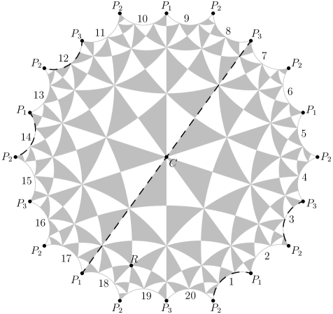
Edge identifications
1	$\leftrightarrow$ 14	5	$\leftrightarrow$ 18	9	$\leftrightarrow$ 2	13	$\leftrightarrow$ 6	17	$\leftrightarrow$ 10
3	$\leftrightarrow$ 12	7	$\leftrightarrow$ 16	11	$\leftrightarrow$ 20	15	$\leftrightarrow$ 4	19	$\leftrightarrow$ 8

Figure 2: Riera and Rodríguez hyperbolic model, $H$, of Bring’s curve.

For future calculations it will also be very useful to know the conformal structure (or equivalently, the local holomorphic coordinate) about the points $P_{1}$, $P_{2}$ and $P_{3}$. This can be reconstructed quite easily from Fig. 2. For example, start near $P_{1}$ in the bottom right quadrant on edge $2/9$. Make a small arc around $P_{1}$ proceeding anticlockwise and you will next reach edge $1/14$. Repeating at edge 14 tells us that we next meet $6/13$. If this procedure is continued we obtain Fig. 3.

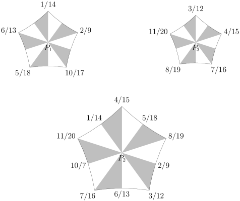
Figure 3: Conformal structure of $P_{1}$, $P_{2}$ and $P_{3}$.

The polygon can be tiled by 120 double triangles (one can take a sector of the central pentagon as a fundamental domain). Now consider the automorphism group. Let $d$ be a rotation of $\frac{\pi}{2}$ about a vertex of the central pentagon and $c$ be a rotation of $\pi$ about the midpoint of an adjacent pentagon edge. Then clearly $c^{2}=d^{4}=1$. But it is also easy to see that $cd$ is a rotation of $\frac{2\pi}{5}$ about the centre and hence $(cd)^{5}=1$. The rotations $c$ and $d$ are thus the classical generators of $S_{5}$ and this describes the entire automorphism group of Bring’s curve.

Riera and Rodríguez give the homology basis for this model by prescribing which edges of the polygon to traverse. We are going to construct an equivalent basis for the HK curve by understanding an isomorphism

$$f:\ H\rightarrow\left\{(x,y,z)\in\mathbb{C}^{3}:\mathcal{C}(x,y,z)=0\right\}$$ (4.1)

well enough to determine the precise values to which each edge of the polygon in Fig. 2 maps. Once this is achieved, converting the homology basis will be a purely mechanical affair as illustrated in [2] for Klein’s curve. Along the way we will gain some understanding of how $f$ acts on the automorphism group by push-forwards.

4.2 Riera and Rodríguez basis

We start by recapitulating the hyperbolic basis of interest. Riera and Rodríguez begin with a simple non-canonical basis. They first define

$$\alpha_{1}=1+2,\qquad\alpha_{2}=3+4$$

(in edge traversal notation, see [16, 17]) and then act on these cycles by rotations of $\frac{2\pi k}{5}$ to obtain their initial basis. So essentially

$$\alpha_{i}=(2i-1)+(2i).$$

Next they specify (by fiat) a matrix which transforms these $\alpha_{i}$ into a canonical basis and proceed to derive further basis change to make use of the symmetries. The end result is the following basis-change matrix (implicit in [17])

$$\begin{pmatrix}1&0&0&0&-2&0&1&0\\ 1&-1&0&-1&-1&1&1&1\\ 1&-1&0&0&-1&2&1&-1\\ 0&-1&0&0&1&2&0&0\\ 1&-1&1&0&-1&1&-1&-1\\ 1&-1&1&-1&0&0&-1&1\\ 1&-1&1&-1&0&1&0&1\\ 0&-1&0&-1&1&1&1&2\end{pmatrix},$$ (4.2)

which sends the initial $\alpha_{1},\dots,\alpha_{8}$ homology basis to another $\{\mathfrak{a}_{i},\mathfrak{b}_{i}\}_{i=1}^{4}$, that is not only canonical but behaves well with respect to the symmetry group of the curve. Now the symmetries relate the periods $\mathcal{A}_{ij}=\int_{\mathfrak{a}_{i}}v_{j}$ and $\mathcal{B}_{ij}=\int_{\mathfrak{b}_{i}}v_{j}$ (for any basis of holomorphic differentials $v_{i}$). As a consequence, the period matrix $\tau=\mathcal{B}\mathcal{A}^{-1}$ can be written as (1.1), where $\tau_{0}\approx-0.5+0.185576\mathrm{i}$ is defined in terms of Klein’s $j$-invariants by

$$j(\tau_{0})=-\frac{29^{3}\times 5}{2^{5}},\qquad j(5\tau_{0})=-\frac{25}{2}.$$ (4.3)

4.3 Understanding the isomorphism $\boldsymbol{f}$

We now turn our attention to the isomorphism, $f$, mentioned in (4.1). Clearly there won’t be a single isomorphism since if $a$ is an automorphism of $H$ and $\sigma$ of an automorphism of the HC curve then $\sigma\circ f\circ a$ will also be an isomorphism from the hyperbolic model $H$ to the HC representation. We will exploit this fact.

There are two key ingredients to our identification. First is the rotation of the entire hyperbolic polygon about its centre by $2\pi/5$ (the automorphism $cd$ above). This automorphism allows us to express all twenty of the polygon’s edges in terms of just four, a great simplification of our problem. If we knew the values of $f$ on four edges, and the matrix representing $f_{*}(cd)$, the induced action of $cd$ on the HC curve, then

$$f(\text{edge }k+4) =f\left((cd)(\text{edge }k)\right)=f_{*}(cd)f(\text{edge }k),$$

which allows us to compute the values of $f$ on the remaining 16 edges.

Second is a geodesic reflection of the hyperbolic disc which will correspond to our real structure; the geodesic is denoted by the dashed lines in Fig. 2. The line starts at $P_{3}$, goes through $C$ to $P_{1}$, along edge 1 to $P_{2}$ and along edge 3 back to $P_{3}$. If we knew how this acted on the HC model, we would know its fixed points correspond in some manner to edges 1/14 and 3/12, and the marked diameter. Identifying points $P_{1}$, $P_{2}$ and $P_{3}$ on the HC representation would then complete the picture by dividing this fixed line up into just the intervals needed to draw homology paths around known branch points.

Starting with the central rotation $cd$ on the hyperbolic model and some isomorphism $f$ to the HC representation, since all order 5 elements of $S_{5}$ are conjugate there is an HC-automorphism ${\sigma}\in S_{5}$ such that

$${\sigma}f_{*}(cd){\sigma}^{-1}=Z^{k},$$

where $k\in\{0,\dots,4\}$ and

$$Z:\ [x,y,z]\mapsto\big{[}\zeta x,\zeta^{2}y,z\big{]}.$$

We are being flexible about which power of $Z$ occurs here because later choices (specifically rotations about $R$ in Fig. 2) will modify any decision made at this stage. But then

$$(\sigma\circ f)_{*}(cd)=\sigma_{*}(f_{*}(cd))=\sigma f_{*}(cd)\sigma^{-1}=Z^{k}.$$

So the isomorphism $\sigma\circ f$ from the hyperbolic model to the HC model sends $cd$ to $Z^{k}$.

Now consider a rotation about $R$ in Fig. 2 which cyclically permutes the fixed points of $cd$. The fixed points on the hyperbolic side are $C$, $P_{1}$, $P_{2}$, $P_{3}$ and on the HC side $[0,1,0]$, $[0,0,1]$, $[1,0,0]_{1}$, $[1,0,0]_{2}$. Let integers $i$ and $n$ be defined by the equations

$$P_{i}=(\sigma\circ f)^{-1}([0,0,1]),\qquad R^{n}(P_{i})=C.$$

Then

$$(\sigma\circ f\circ R^{-n})(C)=(\sigma\circ f\circ R^{-n})(R^{n}(P_{i}))=(\sigma\circ f)(P_{i})=[0,0,1],$$

and further

$$\left(\sigma\circ f\circ R^{-n}\right)_{*}(cd)=(\sigma\circ f)_{*}\left(R^{-n}_{*}(cd)\right)=(\sigma\circ f)_{*}\left((cd)^{j}\right)=Z^{jk}=Z^{m},$$

for some integers $j$ and more importantly $m$. Since we haven’t fixed the power of $Z$ up to now this means that $\sigma\circ f\circ R^{-n}$ serves our purposes just as well as $\sigma\circ f$ did.

Although we have used most of the available freedoms to constrain the relation between $f$, $Z$ and $C$, we actually still have the ability to apply a central rotation, if it would help since that would alter neither of the properties above.

Next consider complex conjugation on the HC model. This is a symmetry that reverses orientation (and so not part of the $S_{5}$ symmetry group). It fixes an entire line (the real axis) including the fixed points of $Z$. In the hyperbolic picture this means it must be a reflection about some diameter. We use our final remaining freedom to demand that it is reflection about the dashed diameter in Fig. 2, i.e. that the real axis in the HC model corresponds to these dashed edges (and diameter).

We now have two tasks remaining:

• Find out what $P_{1}$, $P_{2}$ and $P_{3}$ become on the HC model so we can describe edge 1/14 as the real path from $P_{2}$ to $P_{1}$ and edge 3/12 as the real path from $P_{2}$ to $P_{3}$.

• Find out what power of $Z$ the central rotation of $2\pi/5$ becomes so we can describe (for example) edge 4/15 as $Z^{k}$ applied to the real path from $P_{2}$ to $P_{3}$.

The second task is actually easier to accomplish at this stage. Consider the structure near $[0,0,1]$ (which we demanded was the centre of the polygon, $C$, hyperbolically); there are three sheets coming together at this branch so unwrapping it will effectively divide angles by 3. Mathematically this means that any set of manifold coordinates $\phi:\mathcal{C}\rightarrow\mathbb{C}$ centred on $[0,0,1]$ will satisfy

$$\phi([x,y,1])^{3}=\alpha x+O\big{(}x^{2}\big{)}.$$

In these coordinates, since $[0,0,1]$ is a fixed point $Z:[x,y,z]\mapsto[\zeta x,\zeta^{2}y,z]$ acts locally as a rotation

$$Z_{\phi}(t)=\beta t+O\big{(}t^{2}\big{)},$$

where $\beta$ is characteristic of $Z$ and independent of $\phi$. Now, on the one hand

$$Z_{\phi}\left(\phi([x,y,1])\right)^{3}=\phi\left(Z([x,y,1])\right)^{3}=\phi\big{(}[\zeta x,\zeta^{2}y,1]\big{)}^{3}=\alpha\zeta x+O\big{(}x^{2}\big{)},$$

but also

$$Z_{\phi}\left(\phi([x,y,1])\right)^{3}=\left(\beta\phi([x,y,1])+O\big{(}\phi^{2}\big{)}\right)^{3}=\beta^{3}\phi([x,y,1])^{3}+O\big{(}\phi^{4}\big{)}=\beta^{3}\alpha x+O\big{(}x^{2}\big{)}.$$

So $\beta^{3}=\zeta$, or

$$\beta=\exp\left(\frac{2\pi\mathrm{i}}{15}+\frac{2\pi\mathrm{i}k}{3}\right)$$

for some $k\in\{0,1,2\}$. But since $Z$ has order 5 we also know that $\beta^{5}=1$, which in terms of $k$ means that

$$\frac{2\pi\mathrm{i}}{3}+\frac{10\pi\mathrm{i}k}{3}=\frac{2\pi\mathrm{i}}{3}\left(1+5k\right)\in 2\pi\mathrm{i}\mathbb{Z},$$

or $\beta=\exp(\frac{4\pi\mathrm{i}}{5})$ and at last we can conclude that $Z$ corresponds to a rotation of $2\frac{2\pi\mathrm{i}}{5}$ about $C$ in the hyperbolic model.

Intuitively we have unwrapped the three sheets coming together at $[0,0,1]$ to obtain Fig. 4 in $x$. We know that $Z$ sends (say) $[\epsilon,y,1]$ to $[\zeta\epsilon,y^{\prime},1]$ on some sheet $y^{\prime}$, which makes it one of the labelled destinations. But only one of these gives an order 5 transformation so we know $Z$ completely.

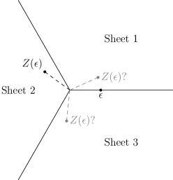
Figure 4: Intuitive action of $Z$ near $[0,0,1]$.

Using this information, together with our knowledge that complex conjugation on the HC model is the dashed reflection in Fig. 2, allows us to deduce the outline structure in Fig. 5. The dots are the branch-points of the HC model and the grey lines are the images of the hyperbolic polygon’s edges under the isomorphism to the HC model. It remains to establish which parts (and sheets) of each spoke in Fig. 5 correspond to which hyperbolic edges (for example, does edge $1/14$ correspond to $x>0$ or $x<0$, and what about $y$?).

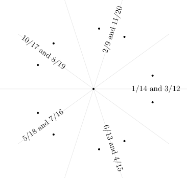
Figure 5: Hyperbolic polygonal edges in the Hulek–Craig model.

Similar analysis of the other fixed points of $Z$ will allow us actually to identify the remaining $P_{i}$. We first discover

• Near $[0,1,0]$, $Z$ is a rotation of $3\left(\frac{2\pi}{5}\right)$.

• Near $[1,0,0]_{1}\sim[1,t^{4},t]$, $Z$ is a rotation of $4\left(\frac{2\pi}{5}\right)$.

• Near $[1,0,0]_{2}\sim[1,t,t^{4}]$, $Z$ is a rotation of $\frac{2\pi}{5}$.

But hyperbolically, it is easy to see that a rotation of $2\left(\frac{2\pi}{5}\right)$ about $C$ (which $Z$ is) is the same as one of $4\left(\frac{2\pi}{5}\right)$ about $P_{1}$, $3\left(\frac{2\pi}{5}\right)$ about $P_{2}$ or $\frac{2\pi}{5}$ about $P_{3}$ so we can deduce that $[0,1,0]\leftrightarrow P_{2}$, $[1,0,0]_{1}\sim[1,t^{4},t]\leftrightarrow P_{1}$ and $[1,0,0]_{2}\sim[1,t,t^{4}]\leftrightarrow P_{3}$.

Therefore, edge $1/14$ corresponds to the real path from $[0,1,0]$ to $[1,0,0]_{1}\sim[1,t^{4},t]$; referring to Fig. 1 we see that this is the path where $y$ starts out large and positive near $x=0$ (and remains positive). Edge 3 corresponds to the real path from $[0,1,0]$ to $[1,0,0]_{2}\sim[1,t,t^{4}]$ which turns out to be the one starting out large and negative near $x=0$ (and remaining negative).

The remaining paths ($y$ small near $x=0$) correspond to the diameter of the hyperbolic model and have no large role to play in describing the homology basis.

Other edges can now be obtained by applying a rotation of $2\pi/5$ on the hyperbolic side and $Z^{3}$ on the HC side. The results are in Table 1.

Table 1: Values for $[x,y,1]$ on hyperbolic edges.

1/14	$[\mathbb{R}_{+},\mathbb{R}_{+},1]$	2/9	$[\zeta\mathbb{R}_{+},\zeta^{2}\mathbb{R}_{+},1]$
3/12	$[\mathbb{R}_{+},\mathbb{R}_{-},1]$	4/15	$[\zeta^{4}\mathbb{R}_{+},\zeta^{3}\mathbb{R}_{-},1]$
5/18	$[\zeta^{3}\mathbb{R}_{+},\zeta\mathbb{R}_{+},1]$	6/13	$[\zeta^{4}\mathbb{R}_{+},\zeta^{3}\mathbb{R}_{+},1]$
7/16	$[\zeta^{3}\mathbb{R}_{+},\zeta\mathbb{R}_{-},1]$	8/19	$[\zeta^{2}\mathbb{R}_{+},\zeta^{4}\mathbb{R}_{-},1]$
10/17	$[\zeta^{2}\mathbb{R}_{+},\zeta^{4}\mathbb{R}_{+},1]$	11/20	$[\zeta\mathbb{R}_{+},\zeta^{2}\mathbb{R}_{-},1]$

4.4 Riera and Rodríguez basis algebraically

We are now in a position to express the Riera and Rodríguez basis on this branched cover. Recall that

$$\alpha_{i}=(2i-1)+(2i)$$

as a prescription on which edges to traverse in the hyperbolic model.

This becomes a specification to look up the relevant edges in Table 1, and construct a path that has its main component in the specified regions (circling $x=0$ and outside all finite branch points enough times to reach the correct sheets). In fact, just like Riera and Rodríguez we only need to construct $\alpha_{1}$ and $\alpha_{2}$ and then repeatedly apply $(x,y)\mapsto(\zeta x,\zeta^{2}y)$ to obtain the rest.

To be explicit and referring to Table 1, $\alpha_{1}$ must go out along $x>0$ with $y\gg 0$ near 0, loop around infinity until it can come back in to $x=0$ along a ray with $\arg x=\frac{2\pi}{5}$ and $\arg y=\frac{4\pi}{5}$ before looping around 0 until it can join up with the beginning again. A path conforming to this description is shown in Fig. 6.

Similarly $\alpha_{2}$ goes out along $x>0$ with $y<0$, loops and comes back with argument of $x$ as $-2\pi/5$ and argument of $y$ as $6\pi/5$; it is also depicted in Fig. 6.

Figure 6: $\alpha_{1}$ and $\alpha_{2}$ homology cycles for the Hulek–Craig branched cover. Graphs of subsequent $\alpha_{i}$ are rotations of these by $\frac{2\pi\mathrm{i}}{5}$.

Using the software introduced in [2] with Klein’s curve as an illustrative example, we may read these paths into extcurves and convert them into a full basis with the commands

> curve, hom, names := read_pic("homology.pic"):
> zeta := exp(2*Pi*I/5):
> trans := (x,y) -> [zeta^3*x,zeta*y]:
> for i from 1 to 3 do
    hom := [op(hom),
            transform_extpath(curve, hom[-2], trans),
            transform_extpath(curve, hom[-1], trans)];
  od:

An immediate check to this calculation is provided by calculating the intersection matrix of this constructed basis. The command

> Matrix(8, (i,j) -> isect(curve, hom[i], hom[j]));

produces (with considerably less work and chance of error) precisely the matrix claimed by Riera and Rodríguez, namely

$$\begin{pmatrix}0&1&-1&1&-1&0&1&-1\\ -1&0&1&-1&1&0&0&0\\ 1&-1&0&1&-1&1&-1&0\\ -1&1&-1&0&1&-1&1&0\\ 1&-1&1&-1&0&1&-1&1\\ 0&0&-1&1&-1&0&1&-1\\ -1&0&1&-1&1&-1&0&1\\ 1&0&0&0&-1&1&-1&0\end{pmatrix}.$$

Finally we can calculate the period matrix. This may be done analytically (as in [17]) or numerically via the extcurves package which calculates the period matrix for any homology basis (implicitly using the Riemann period matrix given by algcurves[periodmatrix]). Using the the transformation from (4.2) both methods yield

Theorem 4.1.

The homology cycles $\alpha_{1}$ and $\alpha_{2}$ for the Hulek–Craig branched cover reproduce the cycles of Riera and Rodríguez and their corresponding period matrix

$$\tau=\tau_{0}\begin{pmatrix}4&1&-1&1\\ 1&4&1&-1\\ -1&1&4&1\\ 1&-1&1&4\end{pmatrix},$$

where $\tau_{0}$ is defined by (4.3).

We also note that the action on the homology basis $\alpha_{1,\ldots,8}$ associated with the antiinvolution of the real structure is given by

$$\mathcal{S}^{\prime}:=\begin{pmatrix}0&0&0&0&0&0&-1&0\\ 0&0&0&0&0&-1&0&0\\ 0&0&0&0&-1&0&0&0\\ 0&0&0&-1&0&0&0&0\\ 0&0&-1&0&0&0&0&0\\ 0&-1&0&0&0&0&0&0\\ -1&0&0&0&0&0&0&0\\ 0&1&0&1&0&1&0&1\end{pmatrix}.$$

It is algorithmic to show that

$$\mathcal{S}:=T\mathcal{S}^{\prime}T^{-1}=\begin{pmatrix}1&0&0&0&1&0&0&0\\ 0&1&0&0&0&1&0&0\\ 0&0&1&0&0&0&1&0\\ 0&0&0&1&0&0&0&1\\ 0&0&0&0&-1&0&0&0\\ 0&0&0&0&0&-1&0&0\\ 0&0&0&0&0&0&-1&0\\ 0&0&0&0&0&0&0&-1\end{pmatrix},$$

where $T$ is the symplectic transformation (with respect to the canonical symplectic form)

$$T=\begin{pmatrix}-1&2&1&2&-1&1&0&1\\ 0&1&0&-3&0&0&0&-1\\ -2&1&2&-1&0&1&0&0\\ 0&0&-1&0&-1&0&-1&0\\ 2&-2&-3&-2&0&-1&-1&-1\\ -1&0&1&3&0&1&0&1\\ 1&-1&-1&-2&0&-1&0&-1\\ -1&2&3&2&0&1&1&1\end{pmatrix}.$$

Here $\mathcal{S}$ is the canonical form for an antiholomorphic involution where there is one nondividing real oval (see for example [18]), again showing there is one real oval.

5 Vector of Riemann constants

We shall now calculate the vector of Riemann constants for Bring’s curve determining various other quantities on the way. This vector together with Riemann’s theta function and the Abel map provide a bridge between the analytic and algebraic structures of a Riemann surface $\mathcal{C}$, and as such are critical elements in the implementation of the modern approach to integrable systems.

5.1 The vector of Riemann constants

Riemann established the fundamental result,

$$\theta(e\,|\,\tau)=0\ \Longleftrightarrow\ e\equiv\mathcal{A}_{Q}\left(\sum_{i=1}^{g-1}P_{i}\right)-K_{Q}\in\mathop{\rm Jac}\nolimits{\mathcal{C}},$$

where $\theta$ is Riemann’s theta function, $\mathcal{A}_{Q}$ is the Abel map with base point $Q\in\mathcal{C}$, $\tau$ is the period matrix, $g$ is the genus of $\mathcal{C}$, $P_{i}\in\mathcal{C}$ and the equivalence holds in the Jacobian $\mathop{\rm Jac}\nolimits\mathcal{C}=\mathbb{C}^{g}/(\mathbb{Z}^{g}+\tau\mathbb{Z}^{g})$. (We are assuming that $g\geq 1$ in what follows.) Both the period matrix $\tau$ and the Abel map depend on a choice of homology basis, the latter through the basis of normalized holomorphic differentials $\boldsymbol{\omega}$ where $\mathcal{A}_{Q}(P)=\int_{Q}^{P}\boldsymbol{\omega}$. The vector $K_{Q}$ is known as the vector of Riemann constants (with base point $Q$) and it also depends on the choice of homology basis. Let ${\left\{\gamma_{i}\right\}_{i=1}^{2g}}=\left\{\mathfrak{a}_{i},\mathfrak{b}_{i}\right\}_{i=1}^{g}$ be our choice of homology basis of $H_{1}(\mathcal{C},\mathbb{Z})$, where $\mathfrak{a}_{i}$ and $\mathfrak{b}_{i}$ are canonically paired. One has that

$$K_{Qj}=-\frac{1}{2}\left(\tau_{jj}+1\right)+\sum_{k\neq j}\oint_{\mathbf{\mathfrak{a}}_{k}}\omega_{k}(P)\int^{P}_{Q}\omega_{j}.$$

Because of the integrations involved, both $\tau$ and $K_{Q}$ are rather transcendental objects. One may also express

$$K_{Q}\equiv\mathcal{A}_{\ast}\left(\Delta-(g-1)Q\right)=\int_{\ast}^{\Delta}{\boldsymbol{\omega}}-(g-1)\int_{\ast}^{Q}{\boldsymbol{\omega}}=\mathcal{A}_{Q}\left(\Delta\right),$$ (5.1)

which holds for any base point $\ast$ of the Abel map and where the degree $(g-1)$ divisor $\Delta$ is that of the Szëgo-kernel [12]. The critical relation for us is the linear equivalence

$$2\Delta\sim\mathcal{K}_{\mathcal{C}},$$

and so

$$2K_{Q}\equiv\mathcal{A}_{Q}(\mathcal{K}_{\mathcal{C}}).$$ (5.2)

Here $\mathcal{K}_{\mathcal{C}}$ is the canonical divisor of $\mathcal{C}$, the unique divisor class of degree $2g-2$ of any meromorphic differential on the curve, and (hereafter) $\sim$ denotes linear equivalence. Thus $\Delta$ gives a square root of the canonical bundle or spin-structure on $\mathcal{C}$; the set $\Sigma$ of divisor classes $\mathcal{D}$ such that $2\mathcal{D}\sim\mathcal{K}_{\mathcal{C}}$ is called the set of theta characteristics of $\mathcal{C}$. The vector of Riemann constants gives us the shift in the Jacobian necessary to identify spin structures with the $2$-torsion points of the Jacobian. (Recall, an $N$-torsion point $x$ is such that $Nx$ lies in the period lattice.)

5.2 Symmetries and the vector of Riemann constants

We now describe how symmetries may be used to restrict the vector of Riemann constants by recalling some results we have established elsewhere.

Suppose that a curve has a nontrivial group of symmetries $\mathop{\rm Aut}\nolimits(\mathcal{C})$. Then the holomorphic differentials of the curve, $H^{1,0}(\mathcal{C},\mathbb{C})$, and the homology group $H_{1}(\mathcal{C},\mathbb{Z})$ are both $\mathop{\rm Aut}\nolimits(\mathcal{C})$-modules. Let $\sigma\in\mathop{\rm Aut}\nolimits(\mathcal{C})$ and denote the actions on these spaces by

$$\sigma^{\ast}v_{j}=\sum_{k}v_{k}{L}^{k}_{j},\qquad\sigma_{\ast}\begin{pmatrix}\mathfrak{a}_{i}\\ \mathfrak{b}_{i}\end{pmatrix}=M\begin{pmatrix}\mathfrak{a}_{i}\\ \mathfrak{b}_{i}\end{pmatrix}:=\begin{pmatrix}{A}&B\\ C&D\end{pmatrix}\begin{pmatrix}\mathfrak{a}_{i}\\ \mathfrak{b}_{i}\end{pmatrix},$$

where ${L}\in GL(g,\mathbb{C})$, $M\in Sp(2g,\mathbb{Z})$ and $\{v_{i}\}$ is a (not necessarily normalized) basis of $H^{1,0}(\mathcal{C},\mathbb{C})$. Denote by $\Pi=\begin{pmatrix}\mathcal{A}\\ \mathcal{B}\end{pmatrix}$ the matrix of periods, where $\mathcal{A}_{ij}=\int_{\mathfrak{a}_{i}}v_{j}$ and $\mathcal{B}_{ij}=\int_{\mathfrak{b}_{i}}v_{j}$. Then $\tau=\mathcal{B}\mathcal{A}^{-1}$ and $\boldsymbol{\omega}=\boldsymbol{v}\mathcal{A}^{-1}$. The identity $\oint_{\sigma_{\ast}\gamma}v=\oint_{\gamma}\sigma^{\ast}v$ (for any $\gamma\in H_{1}(\mathcal{C},\mathbb{Z})$) yields the relation

$$M\Pi=\Pi{L}$$ (5.3)

which restricts the period matrix $\tau$. Now using (5.1) and (5.2) we have that (with $\hat{L}=\mathcal{A}{L}\mathcal{A}^{-1}$, so as to be working with normalized differentials))

$$2K_{Q}\hat{L}\equiv\int_{\ast}^{2\Delta}\sigma^{\ast}{\boldsymbol{\omega}}-2(g-1)\int_{\ast}^{Q}\sigma^{\ast}{\boldsymbol{\omega}}$$

which yields

$$2K_{Q}\big{[}\hat{L}-\mathop{\rm Id}\nolimits\big{]}\equiv\int_{2\Delta}^{\sigma(2\Delta)}{\boldsymbol{\omega}}-2(g-1)\int_{Q}^{\sigma(Q)}{\boldsymbol{\omega}}.$$

If $\mathcal{K}_{\mathcal{C}}$ is the divisor of a differential $v$ then $\sigma^{-1}(\mathcal{K}_{\mathcal{C}})$ is the divisor of $\sigma^{\ast}(v)$, whence the uniqueness of the canonical class means that $\sigma(\mathcal{K}_{\mathcal{C}})\sim\mathcal{K}_{\mathcal{C}}$ and consequently $\sigma(2\Delta)\sim 2\Delta$. This shows that we have an action of $\mathop{\rm Aut}\nolimits(\mathcal{C})$ on the theta characteristics and

$$K_{Q}\hat{L}\equiv K_{\sigma(Q)}+\int_{\Delta}^{\sigma(\Delta)}{\boldsymbol{\omega}},$$

the last integral also being a theta characteristic. We have then the identity on the Jacobian

$$2K_{Q}\left[\hat{L}-\mathop{\rm Id}\nolimits\right]\equiv-2(g-1)\int_{Q}^{\sigma(Q)}{\boldsymbol{\omega}}.$$

This then establishes

Lemma 5.1.

Suppose the automorphism $\sigma$ has order $N>1$. If $L-\mathop{\rm Id}\nolimits$ is invertible and $Q$ is a fixed point of $\sigma$ then $K_{Q}$ is a $2N$-torsion point.

Remark 5.2.

We have the map $\pi:\mathcal{C}\rightarrow\mathcal{C}/\langle\sigma\rangle$. Any holomorphic differential on $\mathcal{C}/\langle\sigma\rangle$ pulls back to an invariant differential on $\mathcal{C}$, and so the assumption that $L-\mathop{\rm Id}\nolimits$ is invertible is equivalent to $\mathcal{C}/\langle\sigma\rangle\cong\mathbb{P}^{1}$.

Corollary 5.3.

Assuming the conditions of Lemma 5.1 and that $\psi\in\mathop{\rm Aut}\nolimits(\mathcal{C})$, then $\int_{Q}^{\psi(Q)}{\boldsymbol{\omega}}$ is a $2N(g-1)$-torsion point.

Although these simple results do not necessarily give the best bound on the order of the torsion point for the vectors involved, we see that, given a suitable symmetry and fixed point, we have that $K_{Q}$ is a torsion point:

$$2K_{Q}\mathcal{A}=\mathbf{n}\Pi\left[L-\mathop{\rm Id}\nolimits\right]^{-1}=\mathbf{n}(M-\mathop{\rm Id}\nolimits)^{-1}\Pi=\mathbf{n}\left(\frac{1}{N}\sum_{k=1}^{N-1}kM^{k}\right)\Pi.$$

The additional (we think) new idea we brought to this was to use some number theory associated with $M$ to restrict the form of $K_{Q}$. Suppose there exist $\mathbf{l}$, $\mathbf{m}\in\mathbb{Z}^{2g}$ such that

$$\mathbf{m}=\mathbf{l}(M-\mathop{\rm Id}\nolimits),$$ (5.4)

then

$$\mathbf{m}\Pi=\mathbf{l}(M-\mathop{\rm Id}\nolimits)\Pi=\mathbf{l}\Pi\left[L-\mathop{\rm Id}\nolimits\right]$$

and

$$\left(2K_{Q}\mathcal{A}+\mathbf{l}\Pi\right)\left[{L}-\mathop{\rm Id}\nolimits\right]=(\mathbf{n}+\mathbf{m})\Pi\in\mathbb{C}^{g}.$$

The idea is to use the freedom in choosing $\mathbf{l}$ here in (5.4) to make $\mathbf{n}+\mathbf{m}$ as simple as possible; as we are only interested in $2K_{Q}$ modulo the lattice we will have further restricted the choice of the vector of Riemann constants. For example, if $\mathbf{m}$ could be chosen arbitrarily then we could make $\mathbf{n}+\mathbf{m}=\mathbf{0}$ and so $2K_{Q}$ would be a lattice point. We implement the idea using the Smith normal form of $M-\mathop{\rm Id}\nolimits$. Recall this means in the present context that we may write

$$M-\mathop{\rm Id}\nolimits=USV,\qquad S=\mathop{\rm Diag}\nolimits(d_{1},\ldots,d_{2g}),\qquad d_{i}|d_{i+1},\qquad U,V\in GL(2g,\mathbb{Z}).$$

The invertibility of $L-\mathop{\rm Id}\nolimits$ means that $d_{i}\geq 1$ and that (5.4) becomes

$$\mathbf{m}V^{-1}=(\mathbf{l}U)S.$$

Here we view $\mathbf{l}^{\prime}=\mathbf{l}U$ as arbitrary and we are interested in the constraints this places on $\mathbf{m}$. We have $(\mathbf{m}V^{-1})_{i}=l_{i}^{\prime}d_{i}$ and clearly the only constraints arise for $d_{i}\neq 1$. Given our earlier observation that here $d_{i}\geq 1$, we find that $\mathbf{m}$ is constrained only by

$$\big{(}\mathbf{m}V^{-1}\big{)}_{i}\equiv 0\mod d_{i},\qquad d_{i}>1.$$

Thus, given a suitable symmetry and fixed point $Q$, the Smith normal form of $M-\mathop{\rm Id}\nolimits$ enables us to restrict the possible torsion points for $2K_{Q}$. Considering further automorphisms and making use of Corollary 5.3 may yield further restrictions. The final step in evaluating $K_{Q}$ is the choice of the appropriate half-period when taking the square root. This again may be restricted by the symmetry but may also be decided numerically from the $2^{2g}$ half-periods.

5.3 Application to Bring’s curve

For Bring’s curve we find that everything follows from study of the single (order 5) automorphism given in the Hulek–Craig representation by

$$\phi:\ [\bar{x},\bar{y},\bar{z}]\mapsto\big{[}\zeta^{2}\bar{x},\zeta^{4}\bar{y},\bar{z}\big{]}.$$

This has fixed point $[0,0,1]$, or $Q=(0,0)$ in affine coordinates.

The first and easiest calculation is deriving its action on the differentials. We fix the ordered basis of (unnormalized) holomorphic differentials

$$v_{1}=\frac{(\bar{y}^{3}-\bar{x})\mathrm{d}\bar{x}}{\partial_{y}\mathcal{C}(\bar{x},\bar{y},1)},\qquad v_{2}=\frac{(\bar{y}^{2}\bar{x}-1)\mathrm{d}\bar{x}}{\partial_{y}\mathcal{C}(\bar{x},\bar{y},1)},\qquad v_{3}=\frac{(\bar{y}-\bar{x}^{2})\mathrm{d}\bar{x}}{\partial_{y}\mathcal{C}(\bar{x},\bar{y},1)},\qquad v_{4}=\frac{\bar{y}(\bar{x}^{2}-\bar{y})\mathrm{d}\bar{x}}{\partial_{y}\mathcal{C}(\bar{x},\bar{y},1)}.$$

The construction of such holomorphic differentials is algorithmic (see [7]). It is easy to check that

$$\phi^{*}(v_{1})=\zeta v_{1},\qquad\phi^{*}(v_{2})=\zeta^{4}v_{2},\qquad\phi^{*}(v_{3})=\zeta^{3}v_{3},\qquad\phi^{*}(v_{4})=\zeta^{2}v_{4},$$

and so $\phi^{\ast}v_{j}=v_{k}{L}^{k}_{j}$ where

$${L}=\begin{pmatrix}\zeta&0&0&0\\ 0&\zeta^{4}&0&0\\ 0&0&\zeta^{3}&0\\ 0&0&0&\zeta^{2}\end{pmatrix}.$$

Thus there is no invariant differential and ${L}-\mathop{\rm Id}\nolimits$ and so $\hat{L}-\mathop{\rm Id}\nolimits$ are invertible. With $Q=(0,0)$ we see the conditions of Lemma 5.1 are satisfied.

We note in passing that the differential $v_{3}$ has a simple zero at $a=[0,0,1]$, a double zero at $b=[0,1,0]$ and a triple triple zero at $c=[1,0,0]_{2}\sim[1,t,t^{4}]$ for the required total of $2g-2=6$. Thus we have $\mathcal{K}_{\mathcal{C}}\sim a+2b+3c$ expressing the canonical divisor in terms of rational points of $\mathcal{C}$.

To proceed with our strategy of determining $K_{Q}$ we first determine the action of $\phi$ on the homology cycles. With the program extcurves at hand this is a simple computational matter, complicated only slightly by the noncanonical nature of the paths we obtained in Section 4.4. We obtain $\phi_{*}(\gamma_{i})=\sum_{j}M_{ij}\gamma_{j}$ where

$$M=\begin{pmatrix}0&0&0&1&0&0&0&0\\ -1&0&0&-1&0&0&0&0\\ 0&-1&0&1&0&0&0&0\\ 0&0&-1&-1&0&0&0&0\\ 0&0&0&0&-1&1&-1&1\\ 0&0&0&0&-1&0&0&0\\ 0&0&0&0&0&-1&0&0\\ 0&0&0&0&0&0&-1&0\end{pmatrix}.$$

We remark that consideration of the equation (5.3) for this order five symmetry already imposes that

$$\mathcal{A}^{T}=\begin{pmatrix}a_{1}&0&0&0\\ 0&a_{2}&0&0\\ 0&0&a_{3}&0\\ 0&0&0&a_{4}\end{pmatrix}\begin{pmatrix}1&-1-\zeta^{4}&1+\zeta^{4}+\zeta^{3}&\zeta\\ 1&-1-\zeta&1+\zeta+\zeta^{2}&\zeta^{4}\\ 1&-1-\zeta^{2}&1+\zeta^{2}+\zeta^{4}&\zeta^{3}\\ 1&-1-\zeta^{3}&1+\zeta^{3}+\zeta&\zeta^{2}\end{pmatrix},$$

for some unknown $a_{i}$. These $a_{i}$ are related by the remaining symmetries and ultimately the period matrix (1.1).

Continuing with our determination of $K_{Q}$, calculating the Smith normal form of $M-1$ gives us unimodular matrices $U$, $V$ such that

$$M-\mathop{\rm Id}\nolimits=U\mathop{\rm Diag}\nolimits(1,1,1,1,1,1,5,5)V$$

and our earlier constraint $(\mathbf{m}V^{-1})_{i}\equiv 0\mod d_{i}$, $d_{i}>1$ takes the form

$$-m_{5}+m_{6}-m_{7}-4m_{8}\equiv 0\pmod{5},$$

$$-m_{1}+2m_{2}-3m_{3}-m_{4}-11m_{5}+6m_{6}-m_{7}-34m_{8}\equiv 0\pmod{5}.$$

This gives 25 possible unique candidates for $2K_{Q}$; we can vary $n_{i}$ arbitrarily (by adding an appropriate $\mathbf{l}$) without essentially changing $2K_{Q}$ for (say) $i=2,3,4,6,7,8$ but then $n_{1}$ and $n_{5}$ are fixed. Explicitly, every $2K_{Q}$ is equivalent to one generated by

$$\mathbf{n}=\begin{pmatrix}n_{1}&0&0&0&n_{5}&0&0&0\end{pmatrix}.$$

By considering a further symmetry we find further that $n_{1}=n_{5}=3$ and at this stage we have

$$2K_{Q}=\frac{1}{5}\begin{pmatrix}-12&-3&3&-3\end{pmatrix}+\tau_{0}\begin{pmatrix}-6&-6&3&0\end{pmatrix}.$$

To determining the appropriate 2-torsion point for square root of the canonical bundle one could further study the action of the symmetries on the spin structures or simply numerically test the vanishing of the theta function. The latter approach yields that

Theorem 5.4.

For the Riera and Rodríguez homology basis of Bring’s curve we have that the vector of Riemann constants is

$$K_{Q}=\frac{1}{10}\begin{pmatrix}3&2&-2&-3\end{pmatrix}+\mathop{\rm Im}\nolimits(\tau_{0})\begin{pmatrix}1&-2&-2&1\end{pmatrix}\mathrm{i},$$

where $\tau_{0}$ is defined by (4.3).

The transformation of theta characteristics

$$\mathfrak{g}\cdot(\boldsymbol{a},\boldsymbol{b})=(\boldsymbol{a},\boldsymbol{b})\mathfrak{g}^{-1}+\frac{1}{2}\big{(}\mathrm{diag}\big{(}CD^{T}\big{)},\mathrm{diag}\big{(}AB^{T}\big{)}\big{)}$$

for any $\mathfrak{g}=\left(\begin{array}[]{cc}A&B\\ C&D\end{array}\right)\in\mathrm{Sp}(2g,\mathbb{Z})$ and characteristic $(\boldsymbol{a},\boldsymbol{b})\in\mathbb{Q}^{2g}$ together with the explicit representations of the symmetries yields

Theorem 5.5.

Bring’s curve has a unique invariant spin-structure.

Remark 5.6.

Klein’s curve has a unique invariant spin structure [14] and we have shown elsewhere that the vector of Riemann constants is the Abel image of this. To show the analogous result for Bring’s curve requires a better understanding of this spin-structure.

Acknowledgements

We are grateful to Maurice Craig for helpful email exchanges and also to an anonymous referee for careful reading and suggested improvements to the paper.

References

- [1] Berndt B.C., Ramanujan’s notebooks. Part III, Springer-Verlag, New York, 1991.
- [2] Braden H.W., Northover T.P., Klein’s curve, J. Phys. A: Math. Theor. 43 (2010), 434009, 17 pages, arXiv:0905.4202.
- [3] Breuer T., Characters and automorphism groups of compact Riemann surfaces, London Mathematical Society Lecture Note Series, Vol. 280, Cambridge University Press, Cambridge, 2000.
- [4] Bujalance E., Etayo J.J., Gamboa J.M., Gromadzki G., Automorphism groups of compact bordered Klein surfaces. A combinatorial approach, Lecture Notes in Mathematics, Vol. 1439, Springer-Verlag, Berlin, 1990.
- [5] Craig M., A sextic Diophantine equation, Austral. Math. Soc. Gaz. 29 (2002), 27–29.
- [6] Craig M., On Klein’s quartic curve, Austral. Math. Soc. Gaz. 31 (2004), 115–120.
- [7] Deconinck B., van Hoeij M., Computing Riemann matrices of algebraic curves, Phys. D 152/153 (2001), 28–46.
- [8] Dye R.H., A plane sextic curve of genus with for collineation group, J. London Math. Soc. 52 (1995), 97–110.
- [9] Edge W.L., Bring’s curve, J. London Math. Soc. 18 (1978), 539–545.
- [10] Edge W.L., Tritangent planes of Bring’s curve, J. London Math. Soc. 23 (1981), 215–222.
- [11] Farkas H.M., Kra I., Riemann surfaces, Graduate Texts in Mathematics, Vol. 71, Springer-Verlag, New York, 1980.
- [12] Fay J.D., Theta functions on Riemann surfaces, Lecture Notes in Mathematics, Vol. 352, Springer-Verlag, Berlin, 1973.
- [13] Hulek K., Geometry of the Horrocks–Mumford bundle, in Algebraic Geometry, Bowdoin, 1985 (Brunswick, Maine, 1985), Proc. Sympos. Pure Math., Vol. 46, Amer. Math. Soc., Providence, RI, 1987, 69–85.
- [14] Kallel S., Sjerve D., Invariant spin structures on Riemann surfaces, Ann. Fac. Sci. Toulouse Math. (6) 19 (2010), 457–477, math.GT/0610568.
- [15] Northover T.P., Riemann surfaces with symmetry: algorithms and applications, Ph.D. thesis, Edinburgh University, 2011.
- [16] Rauch H.E., Lewittes J., The Riemann surface of Klein with 168 automorphisms, in Problems in Analysis (Papers Dedicated to Salomon Bochner, 1969), Princeton Univ. Press, Princeton, N.J., 1970, 297–308.
- [17] Riera G., Rodríguez R.E., The period matrix of Bring’s curve, Pacific J. Math. 154 (1992), 179–200.
- [18] Vinnikov V., Selfadjoint determinantal representations of real plane curves, Math. Ann. 296 (1993), 453–479.
- [19] Weber M., Kepler’s small stellated dodecahedron as a Riemann surface, Pacific J. Math. 220 (2005), 167–182.