Colored HOMFLY polynomial via skein theory

Abstract.

In this paper, we study the properties of the colored HOMFLY polynomials via HOMFLY skein theory. We prove some limit behaviors and symmetries of the colored HOMFLY polynomial predicted in some physicists’ recent works.

1. Introduction

The HOMFLY polynomial is a two variables link invariants which was first discovered by Freyd-Yetter, Lickorish-Millet, Ocneanu, Hoste and Przytychi-Traczyk. In V. Jones’s seminal paper [8], he obtained the HOMFLY polynomial by studying the representation of Heck algebra. Given a oriented link $\mathcal{L}$ in $S^{3}$, its HOMFLY polynomial $P_{\mathcal{L}}(q,t)$ satisfies the following crossing changing formula,

(1.1) $$tP_{\mathcal{L}_{+}}(q,t)-t^{-1}P_{\mathcal{L}_{-}}(q,t)=(q-q^{-1})P_{\mathcal{L}_{0}}(q,t)$$

Given an initial value $P_{\text{unknot}}(q,t)=1$, one can obtain the HOMFLY polynomial for a given oriented link recursively through the above formula (1.1).

According to V. Tureav’s work [21], the HOMFLY polynomial can be obtained from the quantum invariants associated with the fundamental representation of the quantum group $U_{q}(sl_{N})$ by letting $q^{N}=t$. From this view, it is natural to consider the quantum invariants associated with arbitrary irreducible representations of $U_{q}(sl_{N})$. Let $q^{N}=t$, we call such two variables invariants as the colored HOMFLY polynomials. See [16] for detail definition of the colored HOMFLY polynomials by quantum group invariants of $U_{q}(sl_{N})$.

The colored HOMFLY polynomial can also be obtained through the satellite knot. Given a framed knot $\mathcal{K}$ and a diagram $Q$ in the skein $\mathcal{C}$ of the annulus, the satellite knot $\mathcal{K}\star Q$ of $\mathcal{K}$ is constructed through drawing $Q$ on the annular neighborhood of $\mathcal{K}$ determined by the framing. We refer to this construction as decorating $\mathcal{K}$ with the pattern $Q$.

The skein $\mathcal{C}$ has a natural structure as the commutative algebra. A subalgebra $\mathcal{C}^{+}\subset\mathcal{C}$ can be interpreted as the ring of symmetric functions in infinitely many variables $x_{1},..,x_{N},..$ [19]. In this context, the Schur function $s_{\lambda}(x_{1},..,x_{N},..)$ corresponding the basis element $Q_{\lambda}\in\mathcal{C}^{+}$ obtained by taking the closure of the idempotent elements $E_{\lambda}$ in Heck algebra [9].

According to Aiston, Lukac et al’s work [1, 10], the colored HOMFLY polynomial of $\mathcal{L}$ with $L$ components labeled by the corresponding partitions $A^{1},..,A^{L}$, can be identified through the HOMFLY polynomial of the link $\mathcal{L}$ decorated by $Q_{A^{1}},..,Q_{A^{L}}$. Denote $\vec{A}=(A^{1},..,A^{L})\in\mathcal{P}^{L}$, the colored HOMFLY polynomial of the link $\mathcal{L}$ can be defined by

(1.2) $$W_{\vec{A}}(\mathcal{L};q,t)=q^{-\sum_{\alpha=1}^{L}k_{A^{\alpha}}w(\mathcal{K}_{\alpha})}t^{-\sum_{\alpha=1}^{L}|A^{\alpha}|w(\mathcal{K}_{\alpha})}\langle\mathcal{L}\star\otimes_{\alpha=1}^{L}Q_{A^{\alpha}}\rangle$$

where $w(\mathcal{K}_{\alpha})$ is the writhe number of the $\alpha$-component $\mathcal{K}_{\alpha}$ of $\mathcal{L}$, the bracket $\langle\mathcal{L}\star\otimes_{\alpha=1}^{L}Q_{A^{\alpha}}\rangle$ denotes the framed HOMFLY polynomial of the satellite link $\mathcal{L}\star\otimes_{\alpha=1}^{L}Q_{A^{\alpha}}$. See Section 4 for details.

In physics literature, the colored HOMFLY polynomials was described as the path integral of the Wilson loops in Chern-Simons quantum field theory [22]. It makes the colored HOMFLY polynomials stay among the central subjects of the modern mathematics and physics. H. Itoyama, A. Mironov, A. Morozov, And. Morozov started a program of systematic study of the colored HOMFLY polynomial with some physical motivations, see [6, 7] and the references in these papers. On one hand, they have obtained some explicit formulas of colored HOMFLY polynomials for some special links. On the other hand, they also proposed some conjectural formulas for the structural properties of the general links. Given a knot $\mathcal{K}$ and a partition $A\in\mathcal{P}$, they defined the following special polynomials

(1.3) $$H_{A}^{\mathcal{K}}(t)=\lim_{q\rightarrow 1}\frac{W_{A}(\mathcal{K};q,t)}{W_{A}(\bigcirc;q,t)}$$

and its dual

(1.4) $$\Delta_{A}^{\mathcal{K}}(q)=\lim_{t\rightarrow 1}\frac{W_{A}(\mathcal{K};q,t)}{W_{A}(\bigcirc;q,t)}.$$

After some concrete calculations, they conjectured

(1.5) $$H_{A}^{\mathcal{K}}(t)=H_{(1)}^{\mathcal{K}}(t)^{|A|}$$

(1.6) $$\Delta_{A}^{\mathcal{K}}(q)=\Delta_{(1)}^{\mathcal{K}}(q^{|A|}).$$

In Section 6, we give a proof of the formula (1.5) which is stated in the following theorem:

Theorem 1.1.

Given $\vec{A}=(A^{1},..,A^{L})\in\mathcal{P}^{L}$ and a link $\mathcal{L}$ with $L$ components $\mathcal{K}_{\alpha},\alpha=1,..,L$, then we have

(1.7) $$H_{\vec{A}}^{\mathcal{L}}(t)=\prod_{\alpha=1}^{L}H_{(1)}^{\mathcal{K}_{\alpha}}(t)^{|A^{\alpha}|}.$$

We mention that this theorem was first proved by K. Liu and P. Peng [13] by the cabling technique. Here, we give two independent simple proofs via skein theory.

As to the formula (1.6), we show that it is incorrect in general, and we find a counterexample: considering the partition $A=(22)$, for the given torus knot $T(2,3)$, a direct calculation shows

(1.8) $$\Delta^{T(2,3)}_{(22)}(q)\neq\Delta^{T(2,3)}_{(1)}(q^{4}).$$

However, we still believe that the formula (1.6) holds for any knot with a given hook partition $A$. In fact, we have proved the following theorem.

Theorem 1.2.

Given a torus knot $T(m,n)$, where $m$ and $n$ are relatively prime. If $A$ is a hook partition. Then we have

(1.9) $$\Delta_{A}^{T(m,n)}(q)=\Delta_{(1)}^{T(m,n)}(q^{|A|}).$$

In [5], S. Gukov and M. Sto$\check{\text{s}}$i$\acute{\text{c}}$ interpreted the knot homology as the physical description of the space of the open BPS states. They found a remarkable ”mirror symmetries” by calculating the colored HOMFLY homology for symmetric and anti-symmetric representations. Decategorified version of these ”mirror symmetries” for colored HOMFLY homology leads to the symmetry of the colored HOMFLY polynomial, see formula (5.20) in [5]. In fact, we have proved the following symmetric property of the colored HOMFLY polynomial $W_{\vec{A}}(\mathcal{L};q,t)$ for any link $\mathcal{L}$.

Theorem 1.3.

Given a link $\mathcal{L}$ with $L$ components and a partition vector $\vec{A}=(A^{1},..,A^{L})\in\mathcal{P}^{L}$, we have the symmetry

(1.10) $$W_{\vec{A}}(\mathcal{L};q^{-1},t)=(-1)^{\|\vec{A}\|}W_{\vec{A}^{t}}(\mathcal{L};q,t).$$

Theorem 1.3 was first proved by K. Liu and P. Peng [13] which was used to derive the conjectural structure of the colored HOMFLY polynomial predicted by Labastida-Mariño-Ooguri-Vafa [12]. In Section 7, we give an independent simple proof of this theorem via skein theory.

Lastly, by the construction of the pattern $Q_{\lambda}\in\mathcal{C}$ and the definition of colored HOMFLY polynomial (1.2), we derive the following symmetry directly.

Theorem 1.4.

Given a link $\mathcal{L}$ with $L$ components and a partition vector $\vec{A}=(A^{1},..,A^{L})\in\mathcal{P}^{L}$, we have

(1.11) $$W_{\vec{A}}(\mathcal{L};-q^{-1},t)=(-1)^{\sum_{\alpha=1}^{L}k_{A^{\alpha}}}W_{\vec{A}^{t}}(\mathcal{L};q,t).$$

The rest of this paper is organized as follows. In Section 2, we gives a brief account of the HOMFLY skein theory and introduce some basic properties of the HOMFLY polynomial which will be used in Section 6. In Section 3, we gather some definitions and formulas related to partitions and symmetric functions, then we introduce the basic elements in the skein of annulus $\mathcal{C}^{+}$, such as the Turaev’s basis and symmetric function basis of $\mathcal{C}^{+}$. In Section 4, we give the definition of the colored HOMFLY polynomials as the HOMFLY satellite invariants decorated by the elements in HOMFLY skein of annulus $\mathcal{C}^{+}$. In Section 5, we introduce the skein theory descriptions of the colored HOMFLY polynomials of torus links as showed by Morton and Manchon [20] and gives the explicit formula of colored HOMFLY polynomial for torus links obtained by X. Lin and H. Zheng [16]. In Section 6, we introduce the definition of the ”special polynomials” and prove the Theorem 1.1 and Theorem 1.2 about the properties of these special polynomials. In the last Section 7, we study the symmetries of the colored HOMFLY polynomials and prove the Theorem 1.3 and Theorem 1.4.

Acknowledgements. This work was supported by China Postdoctoral Science Foundation 2011M500986. The author would like to thank Professor Kefeng Liu for bringing their unpublished paper [15] to his attention. Their work motivates the author to study the HOMFLY skein theory.

2. The Skein models

Given a planar surface $F$, the framed HOMFLY skein $\mathcal{S}(F)$ of $F$ is the $\Lambda$-linear combination of orientated tangles in $F$, modulo the two local relations as showed in Figure 1, where $z=q-q^{-1}$,

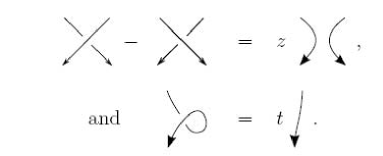
Figure 1.

the coefficient ring $\Lambda=\mathbb{Z}[q^{\pm 1},t^{\pm 1}]$ with the elements $q^{k}-q^{-k}$ admitted as denominators for $k\geq 1$. The local relation showed in Figure 2

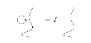
Figure 2.

is a consequence of the above relations. It follows that the removal of a null-homotopic closed curve without crossings is equivalent to time a scalar $\delta=\frac{t-t^{-1}}{q-q^{-1}}$.

2.1. The plane

When $F=\mathbb{R}^{2}$, it is easy to follow that every element in $\mathcal{S}(F)$ can be represented as a scalar in $\Lambda$. For a link $\mathcal{L}$ with diagram $D_{\mathcal{L}}$ the resulting scalar $\langle D_{\mathcal{L}}\rangle\in\Lambda$ is the framed HOMFLY polynomial of link $\mathcal{L}$. In the following, we will also use the notation $\mathcal{L}$ to denote the $D_{\mathcal{L}}$ for simplicity. The unreduced HOMFLY polynomial is obtained by

(2.1) $$\overline{P}_{\mathcal{L}}(q,t)=t^{-w(\mathcal{L})}\langle\mathcal{L}\rangle$$

where $w(\mathcal{L})$ is the writhe of the link $\mathcal{L}$. In particular,

(2.2) $$\overline{P}_{\bigcirc}(q,t)=\langle\bigcirc\rangle=\frac{t-t^{-1}}{q-q^{-1}}.$$

The HOMFLY polynomial is defined by

(2.3) $$P_{\mathcal{L}}(q,t)=\frac{t^{-w(\mathcal{L})}\langle\mathcal{L}\rangle}{\langle\bigcirc\rangle}.$$

Particularly, $P_{\bigcirc}(q,t)=1$.

Remark 2.1.

In some physical literatures, such as [18], the self-writhe $\bar{w}(\mathcal{L})$ instead of $w(\mathcal{L})$ is used in the definition of the HOMFLY polynomial (2.1) and (2.2). The relationship between them is

(2.4) $$w(\mathcal{L})=\bar{w}(\mathcal{L})-2lk(\mathcal{L})$$

where $lk(\mathcal{L})$ is the total linking number of the link $\mathcal{L}$.

A classical result by Lichorish and Millet [11] showed that for a given link $\mathcal{L}$ with $L$ components, the lowest power of $q-q^{-1}$ in the HOMFLY polynomial $P_{\mathcal{L}}(q,t)$ is $1-L$. In fact, they proved the following theorem.

Theorem 2.2 (Lickorish-Millett).

Let $\mathcal{L}$ be a link with $L$ components. Its HOMFLY polynomial has the following expansion

(2.5) $$P_{\mathcal{L}}(q,t)=\sum_{g\geq 0}p^{\mathcal{L}}_{2g+1-L}(t)(q-q^{-1})^{2g+1-L}$$

which satisfies

(2.6) $$p_{1-L}^{\mathcal{L}}(t)=t^{2lk(\mathcal{L})}(t-t^{-1})^{L-1}\prod_{\alpha=1}^{L}p_{0}^{\mathcal{K}_{\alpha}}(t)$$

where $p_{0}^{\mathcal{K}_{\alpha}}(t)$ is the HOMFLY polynomial of the $\alpha$-th component of the link $\mathcal{L}$ with $q=1$, i.e. $p_{0}^{\mathcal{K}_{\alpha}}(t)=P_{\mathcal{K}_{\alpha}}(1,t)$.

By the definition in our notation (2.3), we have

(2.7) $$\langle\mathcal{L}\rangle=\sum_{g\geq 0}\hat{p}^{\mathcal{L}}_{2g+1-L}(t)(q-q^{-1})^{2g-L}$$

where $\hat{p}^{\mathcal{L}}_{2g+1-L}(t)=t^{w(\mathcal{L})}p^{\mathcal{L}}_{2g+1-L}(t)(t-t^{-1})$. Hence

(2.8) $$\hat{p}^{\mathcal{L}}_{1-L}(t)=t^{\bar{w}(\mathcal{L})}(t-t^{-1})^{L}\prod_{\alpha=1}^{L}p_{0}^{\mathcal{K}_{\alpha}}(t)$$

by the formulas (2.4) and (2.6).

We also need another important property of HOMFLY polynomial. Denoted by $\mathcal{K}_{1}\#\mathcal{K}_{2}$ the connected sum of two knots $\mathcal{K}_{1}$ and $\mathcal{K}_{2}$, then we have

(2.9) $$P_{\mathcal{K}_{1}\#\mathcal{K}_{2}}(q,t)=P_{\mathcal{K}_{1}}(q,t)P_{\mathcal{K}_{2}}(q,t).$$

It is equivalent to say

(2.10) $$\frac{\langle\mathcal{K}_{1}\#\mathcal{K}_{2}\rangle}{\langle\bigcirc\rangle}=\frac{\langle\mathcal{K}_{1}\rangle}{\langle\bigcirc\rangle}\frac{\langle\mathcal{K}_{2}\rangle}{\langle\bigcirc\rangle}.$$

2.2. The rectangle

When $F$ is a rectangle with $n$ inputs at the top and $n$ outputs at the bottom. Let $H_{n}$ be the skein $\mathcal{S}(F)$ of $n$-tangles. Composing $n$-tangles by placing one above another induces a product which makes $H_{n}$ into the Hecke algebra $H_{n}(z)$ with the coefficients ring $\Lambda$, where $z=q-q^{-1}$. $H_{n}(z)$ has a presentation generated by the elementary brads $\sigma_{i}$ subjects to the braid relations

(2.11) $$\sigma_{i}\sigma_{i+1}\sigma_{i}=\sigma_{i+1}\sigma_{i}\sigma_{i+1}$$

$$\sigma_{i}\sigma_{j}=\sigma_{j}\sigma_{i},|i-j|\geq 1.$$

and the quadratic relations $\sigma_{i}^{2}=z\sigma_{i}+1$.

2.3. The annulus

When $F=S^{1}\times I$ is the annulus, we let $\mathcal{C}=\mathcal{S}(S^{1}\times I)$. The skein $\mathcal{C}$ has a product induced by placing one annulus outside another, under which $\mathcal{C}$ becomes a commutative algebra. Turaev showed that $\mathcal{C}$ is freely generated as an algebra by the set $\{A_{m}:m\in\mathbb{Z}\}$ where $A_{m},m\neq 0$ is represented by the closure of the braid $\sigma_{|m|-1}\cdots\sigma_{2}\sigma_{1}$. The orientation of the curve around the annulus is counter-clockwise for positive $m$ and clockwise for negative $m$. The element $A_{0}$ is the identity element and is represented by the empty diagram. Thus the algebra $\mathcal{C}$ is the product of two subalgebras $\mathcal{C}^{+}$ and $\mathcal{C}^{-}$ generated by $\{A_{m}:m\in\mathbb{Z},m\geq 0\}$ and $\{A_{m}:m\in\mathbb{Z},m\leq 0\}$.

The closure map $H_{n}\rightarrow\mathcal{C}^{+}$, induced by taking an $n$-tangle $T$ to its closure $\hat{T}$ is a $\Lambda$-linear map, whose image is denoted by $\mathcal{C}_{n}$. Thus $\mathcal{C}^{+}=\cup_{n\geq 0}\mathcal{C}_{n}$. There is a good basis of $\mathcal{C}^{+}$ consisting of closures of certain idempotents of $H_{n}$. In fact, the linear subspace $\mathcal{C}_{n}$ has a useful interpretation as the space of symmetric polynomials of degree $n$ in variables $x_{1},..,x_{N}$, for large enough $N$. $\mathcal{C}^{+}$ can be viewed as the algebra of the symmetric functions.

2.4. Involution on the skein of $F$

The mirror map in the skein of $F$ is defined as the conjugate linear involution $\bar{\quad}$ on the skein of $F$ induced by switching all crossings on diagrams and inverting $q$ and $t$ in $\Lambda$. Thus $\bar{z}=-z$.

3. Basic elements in the skein of annulus $\mathcal{C}^{+}$

3.1. Partition and symmetric function

A partition $\lambda$ is a finite sequence of positive integers $(\lambda_{1},\lambda_{2},..)$ such that

(3.1) $$\lambda_{1}\geq\lambda_{2}\geq\cdots$$

The length of $\lambda$ is the total number of parts in $\lambda$ and denoted by $l(\lambda)$. The degree of $\lambda$ is defined by

(3.2) $$|\lambda|=\sum_{i=1}^{l(\lambda)}\lambda_{i}.$$

If $|\lambda|=d$, we say $\lambda$ is a partition of $d$ and denoted as $\lambda\vdash d$. The automorphism group of $\lambda$, denoted by Aut($\lambda$), contains all the permutations that permute parts of $\lambda$ by keeping it as a partition. Obviously, Aut($\lambda$) has the order

(3.3) $$|\text{Aut}(\lambda)|=\prod_{i=1}^{l(\lambda)}m_{i}(\lambda)!$$

where $m_{i}(\lambda)$ denotes the number of times that $i$ occurs in $\lambda$. We can also write a partition $\lambda$ as

(3.4) $$\lambda=(1^{m_{1}(\lambda)}2^{m_{2}(\lambda)}\cdots).$$

Every partition can be identified as a Young diagram. The Young diagram of $\lambda$ is a graph with $\lambda_{i}$ boxes on the $i$-th row for $j=1,2,..,l(\lambda)$, where we have enumerate the rows from top to bottom and the columns from left to right.

Given a partition $\lambda$, we define the conjugate partition $\lambda^{t}$ whose Young diagram is the transposed Young diagram of $\lambda$ which is derived from the Young diagram of $\lambda$ by reflection in the main diagonal.

Denote by $\mathcal{P}$ the set of all partitions. We define the $n$-th Cartesian product of $\mathcal{P}$ as $\mathcal{P}^{n}=\mathcal{P}\times\cdots\times\mathcal{P}$. The elements in $\mathcal{P}^{n}$ denoted by $\vec{A}=(A^{1},..,A^{n})$ are called partition vectors.

The following numbers associated with a given partition $\lambda$ are used frequently in this paper:

(3.5) $$z_{\lambda} =\prod_{j=1}^{l(\lambda)}j^{m_{j}(\lambda)}m_{j}(\lambda)!,$$

(3.6) $$k_{\lambda} =\sum_{j=1}^{l(\lambda)}\lambda_{j}(\lambda_{j}-2j+1).$$

Obviously, $k_{\lambda}$ is an even number and $k_{\lambda}=-k_{\lambda^{t}}$.

The $m$-th complete symmetric function $h_{m}$ is defined by its generating function

(3.7) $$H(t)=\sum_{m\geq 0}h_{m}t^{m}=\prod_{i\geq 1}\frac{1}{(1-x_{i}t)}.$$

The $m$-th elementary symmetric function $e_{m}$ is defined by its generating function

(3.8) $$E(t)=\sum_{m\geq 0}e_{m}t^{m}=\prod_{i\geq 1}(1+x_{i}t).$$

Obviously,

(3.9) $$H(t)E(-t)=1.$$

The power sum symmetric function of infinite variables $x=(x_{1},..,x_{N},..)$ is defined by

(3.10) $$p_{n}(x)=\sum_{i}x_{i}^{n}.$$

Given a partition $\lambda$, define

(3.11) $$p_{\lambda}(x)=\prod_{j=1}^{l(\lambda)}p_{\lambda_{j}}(x).$$

The Schur function $s_{\lambda}(x)$ is determined by the Frobenius formula

(3.12) $$s_{\lambda}(x)=\sum_{|\mu|=|\lambda|}\frac{\chi_{\lambda}(C_{\mu})}{z_{\mu}}p_{\mu}(x).$$

where $\chi_{\lambda}$ is the character of the irreducible representation of the symmetric group $S_{|\mu|}$ corresponding to $\lambda$. $C_{\mu}$ denotes the conjugate class of symmetric group $S_{|\mu|}$ corresponding to partition $\mu$. The orthogonality of character formula gives

(3.13) $$\sum_{A}\frac{\chi_{A}(C_{\mu})\chi_{A}(C_{\nu})}{z_{\mu}}=\delta_{\mu\nu}.$$

We also have the following Giambelli (or Jacobi-Trudi) formula:

(3.14) $$s_{\lambda}(x) =\det(h_{\lambda_{i}-i+j})_{1\leq i,j\leq l(\lambda)}$$

$$=\det(e_{\lambda^{t}_{i}-i+j})_{1\leq i,j\leq l(\lambda^{t})}.$$

3.2. Turaev’s geometrical basis of $\mathcal{C}^{+}$

The element $A_{m}\in\mathcal{C}^{+}$ is the closure of the braid $\sigma_{m-1}\cdots\sigma_{2}\sigma_{1}\in H_{m}$. Its mirror image $\bar{A}_{m}$ is the closure of the braid $\sigma_{m-1}^{-1}\cdots\sigma_{2}^{-1}\sigma_{1}^{-1}$. Given a partition $\lambda=(\lambda_{1},..,\lambda_{l})$ of $m$ with length $l$, we define the monomial $A_{\lambda}=A_{\lambda_{1}}\cdots A_{\lambda_{l}}$. Then the monomials $\{A_{\lambda}\}_{\lambda\vdash m}$ becomes a basis of $\mathcal{C}_{m}$ which is called the Turaev’s geometric basis of $\mathcal{C}^{+}$.

Moreover, let $A_{i,j}$ be the closure of the braid $\sigma_{i+j}\sigma_{i+j-1}\cdots\sigma_{j+1}\sigma_{j}^{-1}\cdots\sigma_{1}^{-1}$. We define the element $X_{m}$ in $\mathcal{C}_{m}$ as the sum of $m$ closed $m$-braids

(3.15) $$X_{m}=\sum_{j=0}^{m-1}A_{m-1-j,j}.$$

There exist some explicit geometric relations between the elements $\bar{A}_{m}$, $A_{m}$ and $X_{m}$ [20].

3.3. Symmetric function basis of $\mathcal{C}^{+}$

The subalgebra $\mathcal{C}^{+}\subset\mathcal{C}$ can be interpreted as the ring of symmetric functions in infinite variables $x_{1},..,x_{N},..$ [9]. In this subsection, we introduce the elements in $\mathcal{C}^{+}$ representing the complete and elementary symmetric functions $h_{m}$, $e_{m}$ and power sum $P_{m}$.

Given a permutation $\pi\in S_{m}$ with the length $l(\pi)$, let $\omega_{\pi}$ be the positive permutation braid associated to $\pi$. We define two basis quasi-idempotent elements in $H_{m}$:

(3.16) $$a_{m}=\sum_{\pi\in S_{m}}q^{l(\pi)}\omega_{\pi}$$

(3.17) $$b_{m}=\sum_{\pi\in S_{m}}(-q)^{-l(\pi)}\omega_{\pi}$$

The element $h_{m}\in\mathcal{C}_{m}$ which represents the complete symmetric function with degree $m$, is the closure of the elements $\frac{1}{\alpha_{m}}a_{m}\in H_{m}$. Where $\alpha_{m}$ is determined by the equation $a_{m}a_{m}=\alpha_{m}a_{m}$, it gives $\alpha_{m}=q^{m(m-1)/2}\prod_{i=1}^{m}\frac{q^{i}-q^{-i}}{q-q^{-1}}$. Similarly, the closure of the element $\frac{b_{m}}{\beta_{m}}$ gives the elements $e_{m}\in\mathcal{C}_{m}$ represents the elementary symmetric function, where $\beta_{m}=\alpha_{m}|_{q\rightarrow-q^{-1}}$. $\{h_{n}\}$ generates the skein module $\mathcal{C}^{+}$, and the monomial $h_{\lambda}$, where $|\lambda|=m$, form a basis for $\mathcal{C}_{m}$. Then $\mathcal{C}^{+}$ can be regarded as the ring of symmetric functions in variables $x_{1},..,x_{N},..$ with the coefficient ring $\Lambda$. In this situation, $\mathcal{C}_{m}$ consists of the homogeneous functions of degree $m$.

The power sum $P_{m}=\sum x_{i}^{m}$ are symmetric functions which can be represented in terms of the complete symmetric functions, hence $P_{m}\in\mathcal{C}_{m}$. Moreover, we have the identity

(3.18) $$\{m\}P_{m}=X_{m}.$$

where $\{m\}=\frac{q^{m}-q^{-m}}{q-q^{-1}}$. Denoted by $Q_{\lambda}$ the closures of Aiston’s idempotent elements $e_{\lambda}$ in the Hecke algebra $H_{m}$. It was showed by Lukac [9] that $Q_{\lambda}$ represent the Schur functions in the interpretation as symmetric functions. Hence

(3.19) $$Q_{\lambda}=\det(h_{\lambda_{i}+j-i})_{1\leq i,j\leq l}$$

where $\lambda=(\lambda_{1},..,\lambda_{l})$. In particularly, we have $Q_{\lambda}=h_{m}$, when $\lambda=(m)$ is a row partition, and $Q_{\lambda}=e_{m}$ when $\lambda=(1,...,1)$ is a column partition. $\{Q_{\lambda}\}_{\lambda\vdash m}$ forms a basis of $\mathcal{C}_{m}$. Furthermore, the Frobenius formula (3.12) gives:

(3.20) $$Q_{\lambda}=\sum_{\mu}\frac{\chi_{\lambda}(C_{\mu})}{z_{\mu}}P_{\mu}$$

where

(3.21) $$P_{\mu}=\prod_{i=1}^{l(\mu)}P_{\mu_{i}}.$$

4. Colored HOMFLY polynomials

Let $\mathcal{L}$ be a framed link with $L$ components with a fixed numbering. For diagrams $Q_{1},..,Q_{L}$ in the skein model of annulus with the positive oriented core $\mathcal{C}^{+}$, we define the decoration of $\mathcal{L}$ with $Q_{1},..,Q_{L}$ as the link

(4.1) $$\mathcal{L}\star\otimes_{i=1}^{L}Q_{i}$$

which derived from $\mathcal{L}$ by replacing every annulus $\mathcal{L}$ by the annulus with the diagram $Q_{i}$ such that the orientations of the cores match. Each $Q_{i}$ has a small backboard neighborhood in the annulus which makes the decorated link $\mathcal{L}\otimes_{i=1}^{L}Q_{i}$ into a framed link.

The framed colored HOMFLY polynomial of $\mathcal{L}$ is defined to be the framed HOMFLY polynomial of the decorated link $\mathcal{L}\star\otimes_{i=1}^{L}Q_{i}$, i.e.

(4.2) $$\langle\mathcal{L}\star\otimes_{i=1}^{L}Q_{i}\rangle.$$

In particular, when $Q_{A^{\alpha}}\in\mathcal{C}_{d_{\alpha}}$, where $A^{\alpha}$ is the partition of a positive integer $d_{\alpha}$, for $\alpha=1,..,L$. We add a framing factor to eliminate the framing dependency. It makes the framed colored HOMFLY polynomial $\langle\mathcal{L}\otimes_{\alpha=1}^{L}Q_{A^{\alpha}}\rangle$ into a framing independent invariant which is given by

(4.3) $$W_{\vec{A}}(\mathcal{L};q,t)=q^{-\sum_{\alpha=1}^{L}\kappa_{A^{\alpha}}|w(\mathcal{K_{\alpha}})|}t^{-\sum_{\alpha=1}^{L}|A^{\alpha}|w(\mathcal{K}_{\alpha})}\langle\mathcal{L}\star\otimes_{\alpha=1}^{L}Q_{A^{\alpha}}\rangle$$

where $\vec{A}=(A^{1},..,A^{L})\in\mathcal{P}^{L}$.

From now on, we will call $W_{\vec{A}}(\mathcal{L};q,t)$ the colored HOMFLY polynomial of link $\mathcal{L}$ with the color $\vec{A}=(A^{1},..,A^{L})$.

Example 4.1.

The following examples are some special cases of the colored HOMFLY polynomials of links.

(1). The unknot $\bigcirc$,

(4.4) $$W_{A}(\bigcirc;q,t)=\langle Q_{A}\rangle=s_{A}^{*}(q,t)=\sum_{B}\frac{\chi_{A}(C_{B})}{z_{B}}\prod_{j=1}^{l(B)}\frac{t^{B_{j}}-t^{-B_{j}}}{q^{B_{j}}-q^{-B_{j}}}$$

(2). When $A^{1}=A^{2}=\cdots=A^{L}=(1)$,

(4.5) $$W_{((1),..,(1))}(\mathcal{L};q,t) =t^{-\sum_{\alpha}w(\mathcal{K}_{\alpha})}\langle\mathcal{L}\rangle$$

$$=t^{-2lk(\mathcal{L})}\langle\bigcirc\rangle t^{-w(\mathcal{L})}\frac{\langle\mathcal{L}\rangle}{\langle\bigcirc\rangle}$$

$$=t^{-2lk(\mathcal{L})}\left(\frac{t-t^{-1}}{q-q^{-1}}\right)P_{\mathcal{L}}(q,t).$$

(3). When $\mathcal{L}$ is the disjoint union of $L$ knots, i.e. $\mathcal{L}=\otimes_{\alpha=1}^{L}\mathcal{K}_{\alpha}$,

(4.6) $$W_{(A^{1},..,A^{L})}(\mathcal{L};q,t) =q^{-\sum k_{A^{\alpha}}w(\mathcal{K}_{\alpha})}t^{-\sum|A^{\alpha}|w(\mathcal{K}_{\alpha})}\langle\otimes_{\alpha}\mathcal{K}_{\alpha}\star Q_{A^{\alpha}}\rangle$$

$$=\prod_{\alpha}q^{-k_{A^{\alpha}}w(\mathcal{K}_{\alpha})}t^{-|A^{\alpha}|w(\mathcal{K}_{\alpha})}\langle\mathcal{K}_{\alpha}\star Q_{A^{\alpha}}\rangle$$

$$=\prod_{\alpha}W_{A^{\alpha}}(\mathcal{K}_{\alpha};q,t).$$

5. Decorated torus links

Given $T\in\mathcal{C}_{m}$ which is the closure of a $m$-braid $\beta$ such that $T$ has $L$ components and with the $\alpha$-th component consists of $m_{\alpha}$ strings. Thus $\sum_{\alpha=1}^{L}m_{\alpha}=m$. Let $Q_{A^{\alpha}}\in\mathcal{C}_{d_{\alpha}}$ where $A^{\alpha}\vdash d_{\alpha}$. It is clear that $T\star\otimes_{\alpha=1}^{L}Q_{A^{\alpha}}\in\mathcal{C}_{n}$, where $n=\sum_{\alpha=1}^{L}m_{\alpha}d_{\alpha}$. Since $\{Q_{\mu}\}_{\mu\vdash n}$ forms a linear basis of $\mathcal{C}_{n}$ as showed in the last section. We obtain the following expansion

(5.1) $$T\star\otimes_{\alpha=1}^{L}Q_{A^{\alpha}}=\sum_{\mu\vdash n}c_{\lambda}^{\mu}Q_{\mu}$$

Let us consider the cable link diagram $T=T_{mL}^{nL}$ which is the closure of the framed $mL$-braid $(\beta_{mL})^{nL}$, where $(m,n)=1$. The braid $\beta_{m}$ is showed in Figure 3.

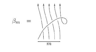
Figure 3.

$T=T_{mL}^{nL}$ induces a map $F_{mL}^{nL}:\otimes_{\alpha=1}^{L}\mathcal{C}_{d_{\alpha}}\rightarrow\mathcal{C}_{m(\sum_{\alpha=1}^{L}d_{\alpha})}$ by taking an element $\otimes_{\alpha=1}^{L}Q_{A^{\alpha}}$ to $T_{mL}^{nL}\star\otimes_{\alpha=1}^{L}Q_{A^{\alpha}}$.

We define $\tau=F^{1}_{1}$, then $\tau$ is the framing change map. It was showed in [20] that

(5.2) $$\tau(Q_{\mu})=\tau_{\mu}Q_{\mu}$$

where $\tau_{\mu}=q^{k_{\mu}}t^{|\mu|}$. The fractional twist map $\tau^{\frac{n}{m}}:\mathcal{C}^{+}\rightarrow\mathcal{C}^{+}$ is the linear map defined on the basis $Q_{\mu}$ by

(5.3) $$\tau^{\frac{n}{m}}(Q_{\mu})=(\tau_{\mu})^{\frac{n}{m}}Q_{\mu}.$$

In order to give an expression for $F^{nL}_{mL}(\otimes_{\alpha=1}^{L}Q_{A^{\alpha}})$, we need to introduce the terminology of $plethysms$. Given a symmetric polynomial in $N$ variables $p(x_{1},..,x_{N})=M_{1}+\cdots+M_{r}$ with $r$ monomials $M_{i}$. Let $q(x_{1},..,x_{r})$ be a symmetric function in $r$ variables. The plethysm $q[p]$ is the symmetric function of $N$ variables $q[p]=q(M_{1},..,M_{r})$. Since $\mathcal{C}^{+}$ is isomorphic to the ring of symmetric functions. Let $Q\in\mathcal{C}^{+}$ and let $P\in\mathcal{C}^{+}$ represent a sum of monomials each with coefficient $1$. We use the notation $Q[P]$ to express the element in $\mathcal{C}^{+}$ corresponding to the plethym of the functions represented by $Q$ and $P$.

We have the following formula which is the link version of the Theorem 13 as showed in [20]

(5.4) $$F_{mL}^{nL}(\otimes_{\alpha=1}^{L}Q_{A^{\alpha}})=\tau^{\frac{n}{m}}(\prod_{\alpha=1}^{L}Q_{A^{\alpha}}[P_{m}]).$$

With the definition of plethsm, we have

(5.5) $$\prod_{\alpha=1}^{L}Q_{A^{\alpha}}[P_{m}]=\sum_{\mu\vdash m\sum_{\alpha=1}^{L}d_{\alpha}}C_{A^{1},..,A^{L}}^{\mu}Q_{\mu}$$

where $C_{A^{1},..,A^{L}}^{\mu}$ are the coefficients given by

(5.6) $$s_{A^{1}}(x_{1}^{m},x_{2}^{m}..,)\cdots s_{A^{L}}(x_{1}^{m},x_{2}^{m},..)=\sum_{\mu\vdash m\sum_{\alpha=1}^{L}d_{\alpha}}C_{A^{1},..,A^{L}}^{\mu}s_{\mu}(x_{1},x_{2},..).$$

By the definition of fractional twist map of $\tau^{\frac{n}{m}}$, we obtain

(5.7) $$F_{mL}^{nL}(\otimes_{\alpha=1}^{L}Q_{A^{\alpha}})=\sum_{\mu\vdash m\sum_{\alpha=1}^{L}d_{\alpha}}C^{\mu}_{A^{1},..,A^{L}}q^{\frac{n}{m}k_{\mu}}t^{n\sum_{\alpha}|A^{\alpha}|}Q_{\mu}.$$

Therefore, by definition (4.3), the colored HOMFLY polynomial of the torus link $T_{mL}^{nL}$ is given by

(5.8) $$W_{A^{1},..,A^{L}}(T_{mL}^{nL};q,t)$$

$$=q^{-m\cdot n\sum_{\alpha=1}^{L}k_{A^{\alpha}}}t^{-n\cdot m\sum_{\alpha=1}^{L}|A^{\alpha}|}\langle F_{mL}^{nL}(\otimes_{\alpha=1}^{L}Q_{A^{\alpha}})\rangle$$

$$=q^{-m\cdot n\sum_{\alpha=1}^{L}k_{A^{\alpha}}}t^{-n(m-1)\sum_{\alpha=1}^{L}|A^{\alpha}|}\sum_{\mu\vdash m\sum_{\alpha=1}^{L}|A^{\alpha}|}C^{\mu}_{A^{1},..,A^{L}}q^{\frac{n}{m}k_{\mu}}W_{\mu}(\bigcirc;q,t)$$

where $W_{\mu}(\bigcirc;q,t)=\langle Q_{\mu}\rangle=s^{*}_{\mu}(q,t)=\sum_{\nu}\frac{\chi_{\mu}(C_{\nu})}{z_{\nu}}\prod_{i=1}^{l(\nu)}\left(\frac{t^{\nu_{i}}-t^{-\nu_{i}}}{q^{\nu_{i}}-q{-\nu_{i}}}\right)$ is the colored HOMFLY polynomial of unknot $\bigcirc$. The coefficients $C_{A^{1},..,A^{L}}^{\mu}$ can be calculated as follows. According to the Frobenuius formula (3.12), we have

(5.9) $$\prod_{\alpha=1}^{L}s_{A^{\alpha}}(x_{1}^{m},x_{2}^{m},..) =\sum_{B^{1},..,B^{L}}\prod_{\alpha=1}^{L}\frac{\chi_{A_{\alpha}}(C_{B^{\alpha}})}{z_{B^{\alpha}}}\prod_{\alpha=1}^{L}P_{mB^{\alpha}}(x_{1},x_{2}..)$$

$$=\sum_{B^{1},..,B^{L}}\prod_{\alpha=1}^{L}\frac{\chi_{A_{\alpha}}(C_{B^{\alpha}})}{z_{B^{\alpha}}}P_{m\sum_{i=1}^{L}B^{i}}(x_{1},x_{2}..)$$

$$=\sum_{B^{1},..,B^{L}}\prod_{\alpha=1}^{L}\frac{\chi_{A_{\alpha}}(C_{B^{\alpha}})}{z_{B^{\alpha}}}\sum_{\mu\vdash m\sum_{\alpha}|B^{\alpha}|}\chi_{\mu}(C_{m\sum_{i=1}^{L}B^{i}})s_{\mu}(x_{1},x_{2},..).$$

It follows that

(5.10) $$C_{A^{1},..,A^{L}}^{\mu}=\sum_{B^{1},..,B^{L}}\prod_{\alpha=1}^{L}\frac{\chi_{A^{\alpha}}(C_{B^{\alpha}})}{z_{B^{\alpha}}}\chi_{\mu}(C_{m\sum_{i=1}^{L}B^{i}}).$$

Example 5.1.

Substituting $L=1$, and the partition $A=(1)$ in formula (5.7), we obtain the following relation in HOMFLY skein $\mathcal{C}_{m}$:

(5.11) $$T_{m}^{n}=T_{m}^{n}\star Q_{(1)}=\sum_{\mu}\chi_{\mu}(C_{(m)})q^{\frac{n}{m}k_{\mu}}t^{n}Q_{\mu}$$

So one has

(5.12) $$W_{(1)}(T^{n}_{m};q,t)=t^{-n(m-1)}\sum_{\mu}\chi_{\mu}(C_{(m)})q^{\frac{n}{m}k_{\mu}}W_{\mu}(\bigcirc;q,t)$$

which is the formula (6.71) showed in [4].

Example 5.2.

Torus knot $T(2,2k+1)$,

(5.13) $$W_{(1)}(q,t) =t^{-(2k+1)}(q^{2k+1}s^{*}_{(2)}(q,t)-q^{-(2k+1)}s^{*}_{(11)}(q,t)),$$

(5.14) $$W_{(2)}(q,t) =t^{-4k-2}(q^{4k+2}s^{*}_{(4)}(q,t)-q^{-4k-2}s^{*}_{(31)}(q,t)+q^{-8k-4}s^{*}_{(22)}(q,t)),$$

(5.15) $$W_{(11)}(q,t) =t^{-4k-2}(q^{4k+2}s^{*}_{(22)}(q,t)-q^{4k+2}s^{*}_{(211)}(q,t)+q^{-4k-2}s^{*}_{(1111)}(q,t)).$$

Example 5.3.

Torus link $T(2,2k)$,

(5.16) $$W_{(1),(1)}(q,t) =q^{2k}s^{*}_{(2)}(q,t)+q^{-2k}s^{*}_{(11)}(q,t),$$

(5.17) $$W_{(2),(1)}(q,t) =q^{4k}s^{*}_{(3)}(q,t)+q^{-2k}s^{*}_{(21)}(q,t).$$

6. Special polynomials

Given a knot $\mathcal{K}$ and a partition $A\in\mathcal{P}$, P. Dunin-Barkowski, A. Mironov, A. Morozov, A. Sleptsov and A. Smirnov [3] defined the following special polynomial

(6.1) $$H_{A}^{\mathcal{K}}(t)=\lim_{q\rightarrow 1}\frac{W_{A}(\mathcal{K};q,t)}{W_{A}(\bigcirc;q,t)}$$

and its dual

(6.2) $$\Delta_{A}^{\mathcal{K}}(q)=\lim_{t\rightarrow 1}\frac{W_{A}(\mathcal{K};q,t)}{W_{A}(\bigcirc;q,t)}.$$

In particular, when $A=(1)$, we have

(6.3) $$H_{(1)}^{\mathcal{K}}(t)=\lim_{q\rightarrow 1}\frac{W_{(1)}(\mathcal{K};q,t)}{W_{(1)}(\bigcirc;q,t)}=P_{\mathcal{K}}(1,t)$$

where $P_{\mathcal{K}}(q,t)$ is the HOMFLY polynomial as defined in (2.3). And

(6.4) $$\Delta_{(1)}^{\mathcal{K}}(q)=\lim_{t\rightarrow 1}\frac{W_{(1)}(\mathcal{K};q,t)}{W_{(1)}(\bigcirc;q,t)}=\Delta_{\mathcal{K}}(q)$$

where $\Delta_{\mathcal{K}}(q)$ is the Alexander polynomial of the knot $\mathcal{K}$.

After testing many examples [3, 6, 7], they proposed the following conjecture.

Conjecture 6.1.

Given a knot $\mathcal{K}$ and partition $A\in\mathcal{P}$, we have the following identities:

(6.5) $$H_{A}^{\mathcal{K}}(t)=H_{(1)}^{\mathcal{K}}(t)^{|A|}$$

(6.6) $$\Delta_{A}^{\mathcal{K}}(q)=\Delta_{(1)}^{\mathcal{K}}(q^{|A|}).$$

In the followings, we give a proof the formula (6.5). In fact, one can generalize the definition of the special polynomial (6.1) for any link $\mathcal{L}$ with $L$ components

(6.7) $$H_{\vec{A}}^{\mathcal{L}}(t)=\lim_{q\rightarrow 1}\frac{W_{\vec{A}}(\mathcal{L};q,t)}{W_{\vec{A}}(\bigcirc^{\otimes L};q,t)}.$$

In fact, the formula (6.5) is the special case of the following theorem.

Theorem 6.2.

Given $\vec{A}=(A^{1},..,A^{L})\in\mathcal{P}^{L}$ and a link $\mathcal{L}$ with $L$ components $\mathcal{K}_{\alpha},\alpha=1,..,L$, then we have

(6.8) $$H_{\vec{A}}^{\mathcal{L}}(t)=\prod_{\alpha=1}^{L}H_{(1)}^{\mathcal{K}_{\alpha}}(t)^{|A^{\alpha}|}.$$

We will give two proofs of Theorem 6.2. The first proof:

Proof.

Choosing a crossing $c$ of the link $\mathcal{L}$, suppose $c$ is a positive crossing, by the skein relation,

(6.9) $$\mathcal{L}(c)=\mathcal{L}(c^{-1})+(q-q^{-1})\mathcal{L}(\upuparrows)$$

It is clear that $\mathcal{L}(c)$ and $\mathcal{L}(c^{-1})$ have the same number of link components.

Considering the degree of $q-q^{-1}$ in the expansion form (2.5) for the HOMFLY polynomial, if the number of the link components for $\mathcal{L}(\upuparrows)$ is not big than $\mathcal{L}(c)$, then taking the limit $q\rightarrow 1$ after the removal of singularity, we have

(6.10) $$\mathcal{L}(c)=\mathcal{L}(c^{-1}).$$

Therefore, with the above rule, one can exchange the crossings between different components of link $\mathcal{L}$, such that $\mathcal{L}=\otimes_{\alpha=1}^{L}\mathcal{K}_{\alpha}$. In this case, as showed in the formula (4.6),

(6.11) $$W_{\vec{A}}(\mathcal{L};q,t)=\prod_{\alpha=1}^{L}W_{A^{\alpha}}(\mathcal{K}_{\alpha};q,t).$$

Similarly, $W_{\vec{A}}(\bigcirc^{\otimes L};q,t)=\prod_{\alpha=1}^{L}W_{A^{\alpha}}(\bigcirc;q,t)$, we obtain

(6.12) $$\lim_{q\rightarrow 1}\frac{W_{\vec{A}}(\mathcal{L};q,t)}{W_{\vec{A}}(\bigcirc^{\otimes L};q,t)}=\prod_{\alpha=1}^{L}\lim_{q\rightarrow 1}\frac{W_{A^{\alpha}}(\mathcal{K}_{\alpha};q,t)}{W_{A^{\alpha}}(\bigcirc;q,t)}.$$

Thus, we only need to consider the case of each knot $\mathcal{K}_{\alpha}$.

One can exchange the crossings which lie in $\mathcal{K}_{\alpha}\star Q_{A^{\alpha}}$ but not in $Q_{A^{\alpha}}$ by the skein relation (6.9). These crossings satisfy the relation (6.10) in the limit $q\rightarrow 1$. Hence

(6.13) $$\mathcal{K}_{\alpha}\star Q_{A^{\alpha}}=\mathcal{K}_{\alpha}\#\mathcal{K}_{\alpha}\#\cdots\#\mathcal{K}_{\alpha}\#Q_{A^{\alpha}}$$

where the righthand side of (6.13) represents the connected sum of $Q_{A^{\alpha}}$ and $|A^{\alpha}|$ knots $\mathcal{K}_{\alpha}$. By the formula (2.10), we have

(6.14) $$\frac{\langle{\mathcal{K}_{\alpha}\star Q_{A^{\alpha}}}\rangle}{\langle\bigcirc\rangle}=\frac{\langle Q_{A^{\alpha}}\rangle}{\langle\bigcirc\rangle}\left(\frac{\langle\mathcal{K}_{\alpha}\rangle}{\langle\bigcirc\rangle}\right)^{|A^{\alpha}|}.$$

Therefore, we obtain

(6.15) $$\lim_{q\rightarrow 1}\frac{W_{A^{\alpha}}(\mathcal{K}_{\alpha};q,t)}{W_{A^{\alpha}}(\bigcirc;q,t)} =\lim_{q\rightarrow 1}\frac{t^{-|A^{\alpha}|w(\mathcal{K}_{\alpha})}\langle\mathcal{K}_{\alpha}\star Q_{A^{\alpha}}\rangle}{\langle Q_{A^{\alpha}}\rangle}$$

$$=\lim_{q\rightarrow 1}\left(\frac{t^{-w(\mathcal{K}_{\alpha})}\langle\mathcal{K}_{\alpha}\rangle}{\langle\bigcirc\rangle}\right)^{|A^{\alpha}|}$$

$$=P_{\mathcal{K}_{\alpha}}(1,t)^{|A^{\alpha}|}$$

which is just the formula (6.7). ∎

The second proof.

Proof.

We only give the proof for the case of a knot $\mathcal{K}$. It is easy to generalize the proof for any link $\mathcal{L}$. Given a partition $A$ with $|A|=d$, by definition

(6.16) $$W_{A}(\mathcal{K};q,t) =q^{-k_{A}w(\mathcal{K})}t^{-dw(\mathcal{K})}\langle\mathcal{K}\star Q_{A}\rangle$$

$$=q^{-k_{A}w(\mathcal{K})}t^{-dw(\mathcal{K})}\sum_{B}\frac{\chi_{A}(B)}{z_{B}}\langle\mathcal{K}\star P_{B}\rangle$$

$$=q^{-k_{A}w(\mathcal{K})}t^{-dw(\mathcal{K})}\left(\frac{\chi_{A}(C_{(1^{d})})}{z_{(1^{d})}}\langle\mathcal{K}\star P_{(1^{d})}\rangle+\sum_{l(B)\leq d-1}\frac{\chi_{A}(C_{B})}{z_{B}}\langle\mathcal{K}\star P_{B}\rangle\right)$$

and

(6.17) $$s_{A}^{*}(q,t) =\sum_{B}\frac{\chi_{A}(B)}{z_{B}}\prod_{j=1}^{l(B)}\frac{t^{B_{j}}-t^{-B_{j}}}{q^{B_{j}}-q^{-B_{j}}}$$

$$=\left(\frac{\chi_{A}(C_{(1^{d})})}{z_{(1^{d})}}\left(\frac{t-t^{-1}}{q-q^{-1}}\right)^{d}+\sum_{l(B)\leq d-1}\frac{\chi_{A}(C_{B})}{z_{B}}\prod_{j=1}^{l(B)}\frac{t^{B_{j}}-t^{-B_{j}}}{q^{B_{j}}-q^{-B_{j}}}\right)$$

By the formula (3.21), it is clear that

(6.18) $$\mathcal{K}\star P_{(1^{d})}=\mathcal{K}\star P_{(1)}\cdots P_{(1)}$$

and the number of the link components is $L(\mathcal{K}\star P_{(1)}\cdots P_{(1)})=d$. For $|B|=d$, with $l(B)\leq d-1$, the number of the link components $L(\mathcal{K}\star P_{B})$ is less than $d-1$.

According to the expansion formula (2.7), we have

(6.19) $$\langle\mathcal{K}\star P_{(1^{d})}\rangle=\sum_{g\geq 0}\hat{p}_{2g+1-d}^{\mathcal{K}\star P_{(1^{d})}}(t)(q-q^{-1})^{2g-d}$$

and for $l(B)\leq d-1$,

(6.20) $$\langle\mathcal{K}\star P_{B}\rangle=\sum_{g\geq 0}\hat{p}_{2g+1-L(\mathcal{K}\star P_{B})}^{\mathcal{K}\star P_{B}}(t)(q-q^{-1})^{2g-L(\mathcal{K}\star P_{B})}$$

with link components $L(\mathcal{K}\star P_{B})\leq d-1$.

Since $\chi_{A}(C_{(1^{d})})\neq 0$, by a direct calculation, we obtain

(6.21) $$\lim_{q\rightarrow 1}\frac{W_{A}(\mathcal{K};q,t)}{s_{A}^{*}(q,t)}=\frac{t^{-dw(\mathcal{K})}\hat{p}_{0}^{\mathcal{K}\star P_{(1^{d})}}(t)}{(t-t^{-1})^{d}}$$

According to the formula (2.8)

(6.22) $$\hat{p}_{0}^{\mathcal{K}\star P_{(1^{d})}}(t) =t^{\bar{w}(\mathcal{K}\star P_{(1^{d})})}(t-t^{-1})^{d}(p_{0}^{\mathcal{K}}(t))^{d}.$$

Moreover, it is clear that $\bar{w}(\mathcal{K}\star P_{(1^{d})})=dw(\mathcal{K})$, thus

(6.23) $$\lim_{q\rightarrow 1}\frac{W_{A}(\mathcal{K};q,t)}{s_{A}^{*}(q,t)}=p_{0}^{\mathcal{K}}(t)^{d}=P_{\mathcal{K}}(1,t)^{d}.$$

∎

Example 6.3.

For the torus knot $T(2,2k+1)$. Its HOMFLY polynomial is

(6.24) $$P_{T(2,2k+1)}(q,t)=\left(\frac{q^{2k+2}-q^{-2k-2}}{q^{2}-q^{-2}}t^{-2k}-\frac{q^{2k}-q^{-2k}}{q^{2}-q^{-2}}t^{-2k-2}\right).$$

Hence

(6.25) $$P_{T(2,2k+1)}(1,t)=(k+1)t^{-2k}-kt^{-2k-2}.$$

By formulas (5.13), (5.14) and (5.15), we obtain

(6.26) $$\lim_{q\rightarrow 1}\frac{W_{(1)}(q,t)}{s^{*}_{(1)}(q,t)} =\frac{1}{2}t^{-2-2k}(1+t^{2}+(2k+1)(t^{2}-1))=P_{T(2,2k+1)}(1,t)$$

(6.27) $$\lim_{q\rightarrow 1}\frac{W_{(2)}(q,t)}{s^{*}_{(2)}(q,t)} =\frac{1}{4}t^{-4-4k}(1+t^{2}+(2k+1)(t^{2}-1))^{2}=P_{T(2,2k+1)}(1,t)^{2}$$

(6.28) $$\lim_{q\rightarrow 1}\frac{W_{(11)}(q,t)}{s^{*}_{(11)}(q,t)} =\frac{1}{4}t^{-4-4k}(1+t^{2}+(2k+1)(t^{2}-1))^{2}=P_{T(2,2k+1)}(1,t)^{2}$$

As to the formula (6.6) in Conjecture 6.1, we found that this formula does not hold for arbitrary partition $A$. Given the torus knot $T(2,3)$, its Alexander polynomial is

(6.29) $$\Delta^{T(2,3)}_{(1)}(q)=\Delta_{2}-1.$$

where we have used the notation $\Delta_{d}=q^{d}-q^{-d}$. Considering the partition $A=(22)$, we have

(6.30) $$\Delta^{T(2,3)}_{(22)}(q) =\lim_{t\rightarrow 1}\frac{W_{(22)}(q,t)}{s^{*}_{(22)}(q,t)}$$

$$=8-7\Delta_{4}-\Delta_{6}+6\Delta_{8}+2\Delta_{10}-5\Delta_{12}$$

$$-2\Delta_{14}+3\Delta_{16}+\Delta_{18}-\Delta_{20}-\Delta_{22}$$

$$\neq\Delta^{T(2,3)}_{(1)}(q^{4}).$$

However, we believe that the formula (6.6) holds for any knots when $A$ is a hook partition. In fact, we have proved the following theorem.

Theorem 6.4.

Given a torus knot $T(m,n)$, where $m$ and $n$ are relatively prime. If $A$ is a hook partition, then we have

(6.31) $$\Delta_{A}^{T(m,n)}(q)=\Delta_{(1)}^{T(m,n)}(q^{|A|}).$$

Every hook partition can be presented as the form $(a+1,1,...,1)$ with $b+1$ length for some $a,b\in\mathbb{Z}_{\geq 0}$, denoted by $(a|b)$.

Before to prove this theorem, we need to introduce the following lemma first.

Lemma 6.5.

Given a partition $B$, we have the following identity,

(6.32) $$\sum_{a+b+1=|B|}\chi_{(a|b)}(C_{B})(-1)^{b}u^{a-b}=\frac{\prod_{j=1}^{l(B)}(u^{B_{j}}-u^{-B_{j}})}{u-u^{-1}}.$$

Proof.

According to problem 14 at page 49 of [17], taking $t=u$, we have

(6.33) $$\prod_{i}\frac{1-u^{-1}x_{i}}{1-ux_{i}}=E(-u^{-1})H(u)=1+(u-u^{-1})s_{(a|b)}(x)(-1)^{b}u^{a-b}$$

since $s_{(a|b)}(x)=\sum_{\lambda}\frac{\chi_{(a|b)}(C_{\lambda})}{z_{\lambda}}p_{\lambda}(x)$, and

(6.34) $$E(-u^{-1})H(u) =\frac{H(u)}{H(u^{-1})}$$

$$=\exp\left(\sum_{r\geq 1}\frac{p_{r}(x)}{r}(u^{r}-u^{-r})\right)$$

$$=\prod_{r\geq 1}\exp\left(\frac{p_{r}(x)}{r}(u^{r}-u^{-r})\right)$$

$$=\prod_{r\geq 1}\sum_{m_{r}\geq 0}\frac{p_{r}(x)^{m_{r}}(u^{r}-u^{-r})^{m_{r}}}{r^{m_{r}}m_{r}!}$$

$$=\sum_{\lambda}\frac{p_{\lambda}(x)}{z_{\lambda}}\prod_{j=1}^{l(\lambda)}(u^{\lambda_{j}}-u^{-\lambda_{j}})$$

Comparing the coefficients of $p_{B}(x)$ in (6.34), the formula (6.32) is obtained. ∎

In the following, we assume $A$ and $B$ are two partitions of $d$ and $\mu$ is a partition of $md$. By the property of character theory of symmetric group, one has

(6.35a) $$\chi_{A}(C_{(d)})= (-1)^{b}, A (a|b)$$ if is a hook partition

$$\chi_{A}(C_{(d)})= 0,$$ otherwise

The following formula is a consequence of Lemma 6.5,

(6.36) $$\sum_{\mu}\chi_{\mu}(C_{mB})\chi_{\mu}(C_{(md)})q^{\frac{n}{m}k_{\mu}} =\sum_{a^{\prime}+b^{\prime}+1=md}\chi_{(a^{\prime}|b^{\prime})}(C_{mB})(-1)^{b^{\prime}}q^{\frac{n}{m}(a^{\prime}-b^{\prime})md}$$

$$=\frac{\prod_{j=1}^{l(B)}(q^{mndB_{j}}-q^{-mndB_{j}})}{q^{nd}-q^{-nd}}.$$

Given a hook partition $A=(a|b)$, according to Lemma 6.5, we also have

(6.37) $$\sum_{B}\frac{\chi_{(a|b)}(C_{B})}{z_{B}}\prod_{j=1}^{l(B)}(q^{mndB_{i}}-q^{mndB_{i}})$$

$$=\sum_{B}\frac{\chi_{(a|b)}(C_{B})}{z_{B}}(q^{mnd}-q^{-mnd})\sum_{\hat{a}+\hat{b}+1=d}\chi_{(\hat{a}|\hat{b})}(C_{B})(-1)^{\hat{b}}(q^{mnd})^{(\hat{a}-\hat{b})}$$

$$=(q^{mnd}-q^{-mnd})(-1)^{b}q^{mnd(a-b)}.$$

where we have used the orthogonal relation

(6.38) $$\sum_{B}\frac{\chi_{A^{1}}(C_{B})\chi_{A^{2}}(C_{B})}{z_{B}}=\delta_{A^{1}A^{2}}.$$

Now we can give a proof of Theorem 6.4.

Proof.

Since $A=(a|b)$ is a hook partition of $d$, i.e $a+b+1=d$. So $k_{(a|b)}=(a-b)d$. By the formula (4.4), so we get

(6.39) $$s_{(a|b)}^{*}(q,t)=\frac{(-1)^{b}}{d}\left(\frac{t^{d}-t^{-d}}{q^{d}-q^{-d}}\right)+\sum_{\begin{subarray}{c}B\vdash d\\ l(B)\geq 2\end{subarray}}\frac{\chi_{(a|b)}(C_{B})}{z_{B}}\prod_{j=1}^{l(B)}\frac{t^{B_{j}}-t^{-B_{j}}}{q^{B_{j}}-q^{-B_{j}}}$$

(6.40) $$W_{(a|b)}(q,t) =q^{-mnd(a-b)}t^{-n(m-1)d}\sum_{B}\frac{\chi_{(a|b)}(C_{B})}{z_{B}}\left(\sum_{\mu}\chi_{\mu}(C_{mB})\chi_{\mu}(C_{(md)})q^{\frac{n}{m}k_{\mu}}\right.$$

$$\left.\cdot\frac{1}{md}\frac{t^{md}-t^{-md}}{q^{md}-q^{-md}}+\sum_{\mu}\chi_{\mu}(C_{mB})\sum_{l(\nu)\geq 2}\frac{\chi_{\mu}(C_{\nu})}{z_{\nu}}q^{\frac{n}{m}k_{\mu}}\prod_{j=1}^{l(\nu)}\frac{t^{\nu_{j}}-t^{-\nu_{j}}}{q^{\nu_{j}}-q^{-\nu_{j}}}\right)$$

Using the L’H$\hat{\text{o}}$pital’s rule and the formulas (6.39) and (6.40), we obtain

(6.41) $$\lim_{t\rightarrow 1}\frac{W_{(a|b)}(q,t)}{s^{*}_{(a|b)}(q,t)}=\frac{\lim_{t\rightarrow 1}\frac{dW_{(a|b)}(q,t)}{dt}}{\lim_{t\rightarrow 1}\frac{ds^{*}_{(a|b)}(q,t)}{dt}}=\frac{(q^{mnd}-q^{-mnd})(q-q^{-1})}{(q^{md}-q^{-md})(q^{nd}-q^{-nd})}=\Delta_{T(n,m)}(q^{d})$$

∎

Example 6.6.

The Alexander polynomial of torus knot $T(2,2k+1)$ is given by

(6.42) $$\Delta_{T(2,2k+1)}(q)=\frac{q^{2k+1}-q^{-2k-1}}{q-q^{-1}}.$$

According to the formulas (5.13),(5.14) and (5.15). We have

(6.43) $$\lim_{t\rightarrow 1}\frac{W_{(1)}(q,t)}{s^{*}_{(1)}(q,t)} =\Delta_{T(2,2k+1)}(q)$$

(6.44) $$\lim_{t\rightarrow 1}\frac{W_{(2)}(q,t)}{s^{*}_{(2)}(q,t)} =\Delta_{T(2,2k+1)}(q^{2})$$

(6.45) $$\lim_{t\rightarrow 1}\frac{W_{(11)}(q,t)}{s^{*}_{(11)}(q,t)} =\Delta_{T(2,2k+1)}(q^{2})$$

Remark 6.7.

It is easy to show that the definition of $\Delta^{\mathcal{K}}_{A}(t)$ can not be generalized to the case of the links like the definition of special polynomial (6.5). This is because the following limit

(6.46) $$\lim_{t\rightarrow 1}\frac{W_{\vec{A}}(\mathcal{L};q,t)}{W_{\vec{A}}(\bigcirc^{\otimes L};q,t)}.$$

may not exist for a general link. Considering the Hopf link $T(2,2)$, according to the formula (5.16), we have

(6.47) $$W_{(1),(1)}(q,t)=q^{2}s^{*}_{(2)}(q,t)+q^{-2}s^{*}_{(11)}(q,t),$$

But the limit

(6.48) $$\lim_{t\rightarrow 1}\frac{W_{(1),(1)}(q,t)}{s_{(1)}^{*}(q,t)s_{(1)}^{*}(q,t)}$$

does not exists for general $t$ by a direct calculation.

7. Symmetries

In this section, we give some symmetric properties of the colored HOMFLY polynomial.

Theorem 7.1.

Given a link $\mathcal{L}$ with $L$ components, and $\vec{A}=(A^{1},..,A^{L})\in\mathcal{P}^{L}$, we have

(7.1) $$W_{\vec{A}}(\mathcal{L};-q^{-1},t)=(-1)^{\sum_{\alpha}k_{A^{\alpha}}}W_{\vec{A}^{t}}(\mathcal{L};q,t)$$

Proof.

For simplicity, we just to show the proof for a given knot $\mathcal{K}$, it is easy to write the proof for a general link $\mathcal{L}$ similarly. Since

(7.2) $$Q_{(d)} =\frac{1}{\alpha_{d}}\sum_{\pi\in S_{d}}q^{l(\pi)}\widehat{\omega_{\pi}},$$

(7.3) $$Q_{(d)^{t}} =\frac{1}{\beta_{d}}\sum_{\pi\in S_{d}}(-q)^{-l(\pi)}\widehat{\omega_{\pi}}.$$

where $\alpha_{d}=\beta_{d}|_{q\rightarrow-q^{-1}}$ by the definition in Section 3.3. Hence

(7.4) $$Q_{(d)}=Q_{(d)^{t}}|_{q\rightarrow-q^{-1}}.$$

It follows that

(7.5) $$\langle\mathcal{K}\star Q_{(d^{1})}Q_{(d^{2})}\cdots Q_{(d^{l})}\rangle=\langle\mathcal{K}\star Q_{(d^{1})^{t}}Q_{(d^{2})^{t}}\cdots Q_{(d^{l})^{t}}\rangle_{q\rightarrow-q^{-1}}$$

Given a partition $\lambda$ with length $l(\lambda)=l$. By the formula (3.19), we get

(7.6) $$Q_{\lambda}=\det(h_{\lambda_{i}+j-i})=\det(Q_{(\lambda_{i}+j-i)})=\sum_{\tau\in S_{l}}(-1)^{sign(\tau)}Q_{(\lambda_{1}+\tau(1)-1)}\cdots Q_{(\lambda_{l}+\tau(l)-l)}.$$

(7.7) $$Q_{\lambda^{t}}=\det(e_{\lambda_{i}+j-i})=\det(Q_{(\lambda_{i}+j-i)^{t}})=\sum_{\tau\in S_{l}}(-1)^{sign(\tau)}Q_{(\lambda_{1}+\tau(1)-1)^{t}}\cdots Q_{(\lambda_{l}+\tau(l)-l)^{t}}.$$

Thus,

(7.8) $$\langle\mathcal{K}\star Q_{\lambda}\rangle=\langle\mathcal{K}\star Q_{\lambda^{t}}\rangle_{q\rightarrow-q^{-1}}.$$

is a consequence of the formula (7.5).

Moreover, by the definition (3.6), $k_{\lambda}$ is an even integer for any partition $\lambda$ and

(7.9) $$k_{\lambda}=-k_{\lambda^{t}}.$$

We obtain

(7.10) $$W_{\lambda}(\mathcal{K};q,t)=(-1)^{k_{\lambda}}W_{\lambda^{t}}(\mathcal{K};-q^{-1},t).$$

∎

Theorem 7.2.

Given a link $\mathcal{L}$ with $L$ components, and $\vec{A}=(A^{1},..,A^{L})\in\mathcal{P}^{L}$, we have the following symmetry:

(7.11) $$W_{\vec{A}}(\mathcal{L};q^{-1},t)=(-1)^{\|\vec{A}\|}W_{\vec{A}^{t}}(\mathcal{L};q,t)$$

Proof.

For simplicity, we just to show the proof for a given knot $\mathcal{K}$, it is easy to write the proof for a general link $\mathcal{L}$ similarly. Given a permutation $\pi\in S_{d}$, we denote $c(\pi)$ the cycle type of $\pi$ which is a partition. It is easy to see that the number of the components of the link $\widehat{\omega_{\pi}}$ is equal to $l(c(\pi))$. Thus the number of the components of the link $\mathcal{K}\star\widehat{\omega_{\pi_{1}}}\cdots\widehat{\omega_{\pi_{l}}}$ is equal to

(7.12) $$L(\mathcal{K}\star\widehat{\omega_{\pi_{1}}}\cdots\widehat{\omega_{\pi_{l}}})=\sum_{i=1}^{l}l(c(\pi_{i})).$$

Before to proceed, we prove the following lemma firstly.

Lemma 7.3.

Given a permutation $\pi\in S_{d}$, we have the following identity

(7.13) $$l(\pi)+l(c(\pi))=d\mod 2$$

Proof.

For every permutation $\pi\in S_{d}$, its length $l(\pi)$ can be obtained by calculating the minimal number of the crossings in the positive braid $\omega_{\pi}$. When $d=2$, we have $S_{2}=\{\pi_{1}=(1)(2),\pi_{2}=(12)\}$. Hence $c(\pi_{1})=(11)$, and $c(\pi_{2})=(2)$. It is clear that

(7.14) $$l(\pi_{1})+l(c(\pi_{1}))=l(\pi_{2})+l(c(\pi_{2}))=2.$$

So Lemma 7.3 holds when $d=2$.

Now we assume Lemma 7.3 holds for $d\leq n-1$. Given a permutation $\pi\in S_{n}$. We first consider the special case, when $\pi$ has the cycle form: $\pi=\pi^{\prime}(n)$, where $\pi^{\prime}$ is a permutation in $S_{n-1}$. It is easy to see that $l(\pi)=l(\pi^{\prime})$ and $l(c(\pi))=l(c(\pi^{\prime}))+1$. By the induction hypothesis, we have

(7.15) $$l(\pi^{\prime})+l(c(\pi^{\prime}))=n-1\mod 2$$

Thus we get

(7.16) $$l(\pi)+l(c(\pi))=n\mod 2.$$

Thus Lemma 7.3 holds for $\pi\in S_{n}$ with the cycle form $\pi^{\prime}(n)$, $\pi^{\prime}\in S_{n-1}$.

For the general case, we can assume $\pi$ has the cycle form $\pi=\sigma\tau$, where $\tau$ is the cycle containing the element $n$ as the form $(i_{1}\cdots i_{j}n)$ for $\{i_{1},..i_{j}\}\subset\{1,..,n-1\}$, $1\leq j\leq n-1$, and $\sigma$ is a cycle in $S_{n-j-1}$. Hence

(7.17) $$l(c(\pi))=l(c(\sigma))+l(c(\tau)).$$

By the property of the permutation, the number of the crossings between $\omega_{\sigma}$ and $\omega_{\tau}$ must be an even number, thus

(7.18) $$l(\pi)=l(\sigma)+l(\tau)+\text{even number}.$$

Combining (7.17), (7.18) and the induction hypothesis, we have

(7.19) $$l(\pi)+l(c(\pi))=n\mod 2.$$

So, we finish the proof of Lemma 7.3. ∎

We now proceed to prove Theorem 7.2. By the definition of $Q_{d}$, we have

(7.20) $$\langle\mathcal{K}\star Q_{(d^{1})}Q_{(d^{2})}\cdots Q_{(d^{l})}\rangle$$

$$=\prod_{i=1}^{l}\frac{1}{\alpha_{d^{i}}}\sum_{\pi_{i}\in S_{d^{i}}}q^{\sum_{i=1}^{l}l(\pi_{i})}\langle\mathcal{K}\star\widehat{\omega_{\pi_{1}}}\cdots\widehat{\omega_{\pi_{l}}}\rangle$$

$$=\prod_{i=1}^{l}\frac{1}{\alpha_{d^{i}}}\sum_{\pi_{i}\in S_{d^{i}}}\hat{p}^{\mathcal{K}\star\widehat{\omega_{\pi_{1}}}\cdots\widehat{\omega_{\pi_{l}}}}_{2g+1-\sum_{i=1}^{l}l(c(\pi_{i}))}(t)(q-q^{-1})^{2g-\sum_{i=1}^{l}l(c(\pi_{i}))}q^{\sum_{i=1}^{l}l(\pi_{i})}$$

(7.21) $$\langle\mathcal{K}\star Q_{(d^{1})^{t}}Q_{(d^{2})^{t}}\cdots Q_{(d^{l})^{t}}\rangle$$

$$=\prod_{i=1}^{l}\frac{1}{\beta_{d^{i}}}\sum_{\pi_{i}\in S_{d^{i}}}(-q)^{-\sum_{i=1}^{l}l(\pi_{i})}\langle\mathcal{K}\star\widehat{\omega_{\pi_{1}}}\cdots\widehat{\omega_{\pi_{l}}}\rangle$$

$$=\prod_{i=1}^{l}\frac{1}{\beta_{d^{i}}}\sum_{\pi_{i}\in S_{d^{i}}}\hat{p}^{\mathcal{K}\star\widehat{\omega_{\pi_{1}}}\cdots\widehat{\omega_{\pi_{l}}}}_{2g+1-\sum_{i=1}^{l}l(c(\pi_{i}))}(t)(q-q^{-1})^{2g-\sum_{i=1}^{l}l(c(\pi_{i}))}(-q)^{-\sum_{i=1}^{l}l(\pi_{i})}$$

By the definition of $\alpha_{d}$ and $\beta_{d}$ as showed in Section 3.3, we have

(7.22) $$\alpha_{d}=\beta_{d}|_{q\rightarrow-q^{-1}}=\beta_{d}|_{q\rightarrow q^{-1}}.$$

Finally, according to Lemma 7.3 and the formulas (7.20), (7.21) and (7.22), one has

(7.23) $$\langle\mathcal{K}\star Q_{(d^{1})}Q_{(d^{2})}\cdots Q_{(d^{l})}\rangle=(-1)^{d^{1}+\cdots d^{l}}\langle\mathcal{K}\star Q_{(d^{1})^{t}}Q_{(d^{2})^{t}}\cdots Q_{(d^{l})^{t}}\rangle_{q\rightarrow q^{-1}}$$

By the definition of $Q_{\lambda}$ and $Q_{\lambda^{t}}$ as showed by formulas (7.6) and (7.7), we obtain

(7.24) $$\langle\mathcal{K}\star Q_{\lambda}\rangle=(-1)^{|\lambda|}\langle\mathcal{K}\star Q_{\lambda^{t}}\rangle_{q\rightarrow q^{-1}}.$$

Since $k_{\lambda}=-k_{\lambda^{t}}$, the identity

(7.25) $$W_{\lambda}(\mathcal{K};q,t)=(-1)^{|\lambda|}W_{\lambda^{t}}(\mathcal{K};q^{-1},t).$$

follows immediately. ∎

References

- [1] A. K. Aiston, Skein theoretic idempotents of Hecke algebras and quantum group invariants. PhD. thesis, University of Liverpool, 1996.
- [2] A. K. Aiston and H. R. Morton, Idempotents of Hecke algebras of type A, J. Knot Theory Ramif. 7 (1998), 463-487.
- [3] P. Dunin-Barkowski, A. Mironov, A. Morozov, A. Sleptsov and A. Smirnov, Superpolynomials for toric knots from evolution induced by cut-and-join operators, arXiv:1106.4305.
- [4] D.-E. Diaconescu, V. Shende and C. Vafa, Large N duality, lagrangian cycles, and algebraic knots, arXiv:1111.6533.
- [5] S. Gukov and M. Stosic, Homological algebra of knots and BPS states, arXiv:1112.0030.
- [6] H. Itoyama, A. Mironov, A. Morozov and An. Morozov, HOMFLY and superpolynomials for figure eight knot in all symmetric and antisymmetric representations, arXiv:1203.5978.
- [7] H. Itoyama, A. Mironov, A. Morozov and An. Morozov, Character expansion for HOMFLY polynomials. III. All 3-Strand braids in the first symmetric representation, arXiv:1204.4785.
- [8] V. Jones, Hecke algebra representations of braid groups and link polynomial, Ann. Math. 126 (1987), 335 C388.
- [9] S. G. Lukac, Idempotents of the Hecke algebra become Schur functions in the skein of the annulus, Math. Proc. Camb. Phil. Soc 138 (2005), 79-96.
- [10] S. G. Lukac, Homfly skeins and the Hopf link. PhD. thesis, University of Liverpool, 2001.
- [11] W. B. R Lickorish and K. C. Millett, A polynomial invariant of oriented links, Topology 26 (1987) 107.
- [12] J.M.F. Labastida, M. Mariño and C. Vafa, Knots, links and branes at large N, J. High Energy Phys. 2000, no. 11, Paper 7.
- [13] K. Liu and P. Peng Proof of the Labastida-Marino-Ooguri-Vafa Conjecture, arXiv:0704.1526.
- [14] K. Liu and P. Peng New Structure of Knot Invariants, arXiv: 1012.2636.
- [15] K. Liu and P. Peng Framed knot and Chern-Simons gauge theory, preprint.
- [16] X.-S. Lin and H. Zheng, On the Hecke algebra and the colored HOMFLY polynomial, math.QA/0601267.
- [17] I. G. MacDolnald, Symmetric functions and Hall polynomials, 2nd edition, Charendon Press, 1995.
- [18] M. Mariño, String theory and the Kauffman polynomial, arXiv: 0904.1088.
- [19] H. R. Morton, Skein theory and the Murphy operators. J. Knot Theory Ramifications 11 (2002), 475 C492.
- [20] H. R. Morton and P. M. G. Manchon, Geometrical relations and plethysms in the Homfly skein of the annulus, J. London Math. Soc. 78 (2008), 305-328.
- [21] V. G. Turaev, The Yang-Baxter equation and invariants of links, Invent. Math. 92(1988), 527-553.
- [22] E. Witten, Quantum field theory and the Jones polynomial, Commun. Math. Phys. 121 (1989) , 351.