Coarse-graining the dynamics of network evolution: the rise and fall of a networked society.

Abstract

We explore a systematic approach to studying the dynamics of evolving networks at a coarse-grained, system level. We emphasize the importance of finding good observables (network properties) in terms of which coarse grained models can be developed. We illustrate our approach through a particular social network model: the “rise and fall” of a networked society [1]: we implement our low-dimensional description computationally using the equation-free approach and show how it can be used to (a) accelerate simulations and (b) extract system-level stability/bifurcation information from the detailed dynamic model. We discuss other system-level tasks that can be enabled through such a computer-assisted coarse graining approach.

1 Introduction

The Erdös-Rényi random graph model [2], dating back to $1959$, constitutes a landmark in the study of graphs. There has been a renewed interest in networks (or graphs) in recent years with more specific focus on complex emergent dynamics, spurred by discoveries such as power-law degree distributions [3, 4], small world behavior [5], and more. Dynamic network evolution models have been developed with an eye towards constructing networks with specific structures/statistical properties; an example is the preferential attachment mechanism [6], proposed as a source of scale-free structure in evolving networks. Evolutionary network models are especially popular (and relevant) in the social sciences [7, 8, 9, 10, 11]. The focus in many of these models is on the correspondence between local mechanisms (rules) of network formation and the resulting large-scale “system level” network structure and dynamics.

In this work, we explore a systematic approach to the computer-assisted study of such models at the macroscopic, coarse-grained, system level as opposed to the detailed, node-level, microscopic level. The basic idea is to estimate the information necessary for coarse-grained computations on the fly, using short bursts of appropriately designed detailed simulations. Based on the selection of suitable coarse variables (observables), this equation-free approach [12, 13] facilitates efficient computation at the coarse-grained level. Accelerating coarse grained evolution computations, and/or enabling additional modeling tasks such as coarse fixed point/bifurcation/stability computations can significantly enhance our understanding of the system behavior at the macroscopic level, even when an explicit coarse grained model is not available. The approach may also help pinpoint collective network properties that are crucial in the evolution process (and could thus be used as coarse variables). The main aim of this paper is to demonstrate how our modeling approach to complex systems dynamics has to be modified and extended in order to be usable in problems involving network evolution. We will focus on a number of issues arising in this new context, like finding the number of slow variables, constructing networks consistent with them, etc.

The paper is structured as follows: In the next section we briefly describe an illustrative network evolution model introduced by Marsili et al [1]. We then discuss certain issues that arise in coarse variable selection, and our chosen coarse-graining approach. Results of the computational implementation of this approach are presented, and we conclude with a discussion of the scope and applicability of our approach, as well as certain important open issues in the selection of coarse variables for general network evolution problems.

2 An illustrative case: the rise and fall of a networked society

We revisit the model of the rise and fall of a networked society [1] presented by Marsili et al. to illustrate our approach. Their model exhibits complex emergent phenomena arising from simple evolution rules; a brief description of these rules follows: Consider a (social) network consisting of $n$ agents (entities) involved in bilateral interactions. The network is represented by $N=(V,E)$, where $V$ is the set of vertices or nodes (agents) and $E$ is the set of edges or links, representing interactions between agents. In any time interval $[t,t+dt)$, the model evolves as follows:

1. Any existing edge $(i,j)\in E$ is removed with probability $\lambda dt$.

2. With independent probability $\eta dt$, every agent $i$ can form a link with (become a neighbor of) a randomly chosen agent $j\neq i$. Nothing occurs if agent $i$ is already a neighbor of (is connected with) agent $j$.

3. With independent probability $\xi dt$, every agent $i$ is allowed to ask a neighbor $j$ (randomly chosen) to introduce him/her to a randomly chosen neighbor of $j$, say agent $k$. If agent $i$ is not already connected to agent $k$, a new edge is formed between $i$ and $k$. Nothing occurs if agent $i$ is already a neighbor of (is connected with) agent $k$.

Figure 1: Bifurcation diagram obtained using direct temporal simulations, reproduced from [1] with permission (copyright $2004$ National Academy of Sciences, U.S.A). Steady state values of average degree, average clustering coefficient and giant component size are plotted against the ratio of parameters, $\xi/\lambda$. $\eta$ and $\lambda$ values were fixed at $0.001$ and $0.1$ respectively. Notice the robustness of the results to the network size.

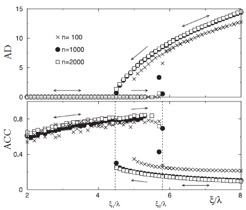
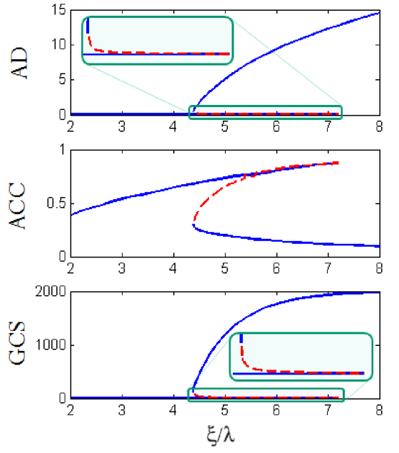
A detailed description of the motivation behind the model and the richness of the resulting dynamics is given in [1]. A numerical bifurcation diagram is also obtained there through extensive direct temporal simulations of the model in different parameter regimes. This bifurcation diagram is reported again in Figure 1, where the average degree (AD) and the average clustering coefficient (ACC) are plotted against a bifurcation parameter (the ratio $\xi/\lambda$). The parameters $\xi$ and $\eta$ represent the rates at which the agents form new connections through their existing friends and through random sampling of the network, respectively; $\lambda$ is the rate at which the connections between agents disappear. To produce this bifurcation plot, $\eta$ and $\lambda$ were fixed at $0.001$ and $0.1$, respectively. The figure suggests generic hysteresis behavior as the parameter $\xi$ is varied. When $\xi\in[\xi_{1},\xi_{2}]$ ($\xi_{1}$ and $\xi_{2}$ are marked in Figure 1), the system can reach two distinct stable steady states depending on the initial condition: (a) a highly connected state with low clustering and (b) a sparsely connected state with high levels of clustering (localization). From dynamical systems theory, one anticipates a branch of unstable steady states (not obtainable by direct simulations) “connecting” (in a coarse-grained bifurcation diagram) these two stable branches. In fact, a mean field approximation which qualitatively reproduces these characteristics of the full model behavior (including the unstable branch) was also reported in [1].

3 Selecting an appropriate low-dimensional description

One of the crucial steps in developing a reduced, coarse-grained description of any complex system is the selection of suitable observables (coarse variables). We borrow simple principles from dynamical systems to help us in this pursuit and to provide the rationale corroborating our coarse variable choices. In order for a system to exhibit low-dimensional behavior, one expects a separation of time-scales to prevail in the evolution of different variables in the system phase space. The basic picture is that low-dimensional subspaces (slow manifolds, parameterized by “slow” variables) contain the long-term dynamics, while fast evolution in the transverse directions (in the “fast” variables) quickly brings the system trajectories close to the (attracting) slow manifolds. Thus, the problem of selecting good coarse variables is translated to the problem of finding a set of variables that successfully parameterize the slow manifold(s), when such a manifold exists.

Figure 2: Phase portrait in terms of giant component size (GCS) and average degree (AD) (left) or average clustering coefficient (ACC) (right) showing transients from a variety of initial conditions. Fast (resp. slow) temporal evolution is indicated by a double (resp. a single) arrow.

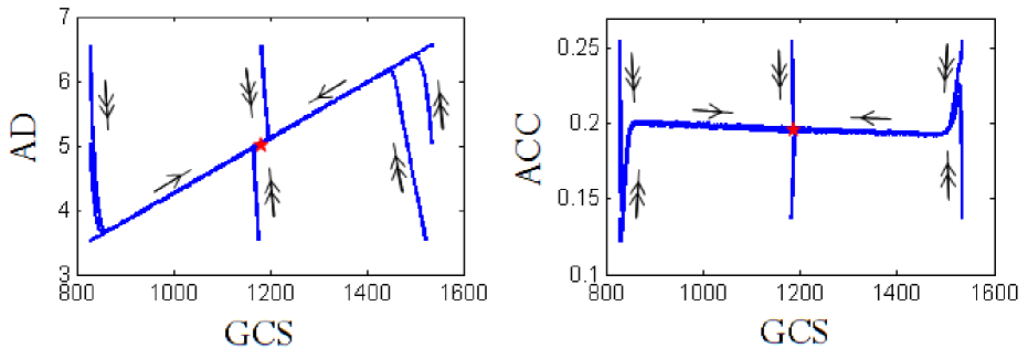
In order to search for such a slow manifold in the context of the rise and fall model, we explore the relevant state space through direct simulations as follows. We first compute the steady (stationary) state of the model (for a fixed set of parameter values) by direct simulations, and evaluate a few network properties at this stationary state. We focus on three typically studied network properties: the giant component size (GCS), the average degree (AD) and the average clustering coefficient (ACC).

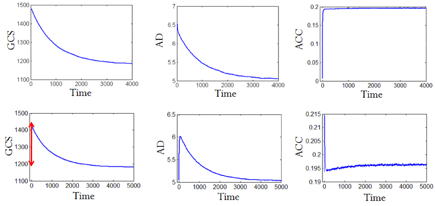
For our simulations, the parameters of the model are taken to be $n=2000$, $\lambda=0.1$, $\eta=0.001$ and $\xi=0.5$. Fig. 2 depicts the phase portrait of AD and ACC versus GCS starting from several different initial conditions. A one-dimensional slow manifold parameterized by the giant component size is clearly suggested by the simulations. The time evolution of these network properties from a random initial condition is shown in the top panels of Fig. 3. It should be noted that, in order to observe smooth trajectories representative of the expected evolution, ensembles of several realizations –typically $100$– are averaged to create these plots. The trajectories suggest that the giant component size and the average degree appear to vary slowly over time, while the average clustering coefficient has a fast initial transient followed by a slower evolution to the steady state.

In order to numerically determine the directions in state space along which the system evolves slowly, we then perturb the system away from the stationary state itself, by varying different sets of network properties, and observe the evolution of the properties of the resulting perturbed networks. In one such perturbation experiment, we construct networks with the stationary degree distribution and average clustering coefficient and perturb the system away from the stationary value of giant component size. We then let the system evolve naturally, and observe, in Fig. 3(bottom), the evolution of the three above-mentioned network properties. The perturbed giant component size varies slowly from its initial value and eventually approaches steady state. The evolution of the average degree and the average clustering coefficient show fast initial transients followed by a slow approach to steady state. These observations suggest that the giant component size may be a “good” slowly evolving variable, to which the average degree and the average clustering coefficient (degree and triangle information) become quickly slaved (and remain slaved during long-time evolution).

Figure 3: Evolution of certain (expected) graph properties: average degree, average clustering coefficient and giant component size. The top panels correspond to evolution from random initial networks, while the initial graphs for the bottom panels were obtained by creating networks exhibiting the stationary degree distribution and the stationary value of ACC. The red arrow indicates the magnitude of our perturbation away from the stationary GCS value.

Figure 4: Evolution of certain (explected) graph properties: average degree, average clustering coefficient and giant component size. The top panels correspond to evolution from initial graphs exhibiting both the stationary degree distribution and the stationary giant component size. The initial graphs for the evolution shown in the bottom panels were constructed to exhibit only the stationary giant component size value. The (red) arrow(s) in each row indicate the magnitude of our perturbation away from the stationary property value(s).

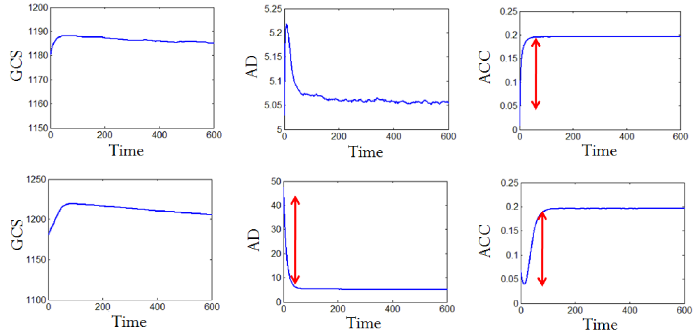
We perform a number of similar numerical perturbation computations that, taken together, reinforce the view that the size of the giant component (a single scalar variable) may be a suitable candidate coarse variable. A couple of such computations supporting this idea are shown in Fig. 4. The top panels show the temporal evolution of (the expected value of) a few network properties from initial networks constructed to exhibit both the stationary giant component size and the stationary degree distribution. We repeat these computational experiments initializing the evolution from networks exhibiting the stationary value of the giant component size only (and not exhibiting the stationary degree distribution). The corresponding evolution results are shown in the bottom panels of Fig. 4. We find that, if we initialize with networks that exhibit the “correct” stationary value of the giant component size, the average degree will quickly evolve to the neighborhood of its stationary value -“come down” on the slow manifold- and will then slowly approach it on the same time scale as the giant component size does. This would suggest that the average degree is a “fast variable”. By the same type of argument, Figs. 3 and 4 suggest that the average clustering coefficient, also, is a fast variable and hence does not need to be explicitly included in a model for the long-term evolution.

In both cases shown in Fig. 4, the giant component size itself has a fast initial evolution window that takes it momentarily away from the steady state value, and then it slowly evolves back towards it (on the slow manifold). While the giant component size is a good candidate coarse variable to parameterize the slow manifold (and the long-term dynamics), these transients indicate that it is not a pure slow variable – its evolution appears to have initial fast as well as slow components. A clear illustration (and explanation) of this behavior, and of the concept of a “pure” slow variable in the context of a simple singularly perturbed problem can be found in the Appendix. These dynamics imply that initializing with a desired value of the giant component size is not sufficient; additional care must be taken to find a network that exhibits this value but also lies close to the slow manifold (explained later below). If the variable was a pure slow one, then just a few simulation steps would guarantee the latter property (lying close to the slow manifold, see again the simple illustration in the Appendix).

4 A coarse-grained model

Once we choose suitable coarse variables, computations at the coarse-grained level are carried out using the equation-free framework [12, 13]. This framework is used to accelerate simulation and also enable the performance of a number of additional tasks (such as fixed point computation and stability analysis) at the coarse-grained level. In this approach, computations involving the coarse variables are performed with the help of suitably defined operators which translate between coarse and fine descriptions. Short bursts of fine scale simulation followed by observation and post-processing of the results at the coarse scale enable on-demand estimation of numerical quantities (residuals, actions of Jacobians, time-derivatives) required for coarse numerics. The operator that transforms coarse variables to the detailed, fine variables is called the lifting operator, $L$, while the operator that transforms fine variables back to coarse variables is called the restriction operator, $R$. One can thus evolve the coarse variables of a system forward in time for a given number of steps $t$ by performing the following operations:

1. Lifting ($L$): Find a set of detailed variables (networks) consistent with the initial value(s) of the coarse variable(s) (here, the giant component size).

2. Microscopic evolution: Evolve the fine variables (the nodes and edges of the networks) for a specified time $t$ using the detailed, microscopic evolution rules of the system.

3. Restriction ($R$): Observe the fine variables, from the final stage(s) of the previous step, at the coarse scale.

These steps constitute what is known as the coarse time-stepper, which acts as a substitute code for the unavailable macroscopic evolution equations of the system. In terms of the lifting and restriction operators, the coarse time-stepper $\Phi_{t}$ can be written in terms of the fine scale evolution operator ($\phi_{t}$) as:

$$\Phi_{t}(\cdot)=R\circ\phi_{t}\circ L(\cdot).$$ (1)

Using this coarse time-stepper in the form of a black-box subroutine, we can “wrap” around it a number of different algorithms (initial value solvers, fixed point solvers, eigensolvers) that perform system-level tasks. In our present example, the microscopic description of system evolution is the model itself, defined in terms of the network structure (fine variables, information about the edges between nodes), while the giant component size is the single coarse variable. Hence, the restriction operation consists of simply evaluating the giant component size of a given network. The lifting operation, however, consists of constructing a network with a specified value of giant component size; this by itself, however, is not sufficient for EF computations, as we need a network that has the specified GCS and lies on or close to the slow manifold.

We show a schematic representing the state space of our dynamical system in Fig. 5. The x-axis represents our coarse variable, the giant component size (GCS), while the y-axis represents the directions corresponding to all other possible variations in the network that do not alter the GCS. The solid (blue) line denotes the slow manifold, which is drawn in a manner suggesting a good one-to-one correspondence with our chosen coarse variable (GCS). The vertical, dashed (black) line represents a family of graphs having the same (prescribed) giant component size. Let’s pick one graph in this family denoted by the (green) point number $1$ and use it as an initial condition in the model we study. If the giant component size were truly a slow variable, the system would “quickly” evolve to a point on the manifold with a giant component size very similar to the starting value. However, as we observed before, the giant component size is not a pure slow variable: as the system dynamics quickly evolves from point $1$ to point $2$, we do approach the slow manifold, yet our giant component size has significantly changed. It is therefore important that our lifting operation constructs networks that not only conform to the prescribed giant component size but also lie close to the slow manifold. In terms of our schematic caricature of Fig. 5, if the vertical line corresponds to the required value of GCS and the lifting operation is required to produce a graph close to point $D$. The issue of initializing on the slow manifold is a crucial one in many scientific contexts that involve model reduction (e.g. in meteorology, [14]) and algorithms for accomplishing it in a dynamical systems context are the subject of current research (see e.g. [15, 16]).

4.1 Our Lifting Operator

Figure 5: Schematic of our lifting procedure to create graphs with a specified giant component size which also lie close to the slow manifold. The process begins with the network labeled $1$.

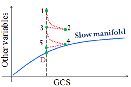
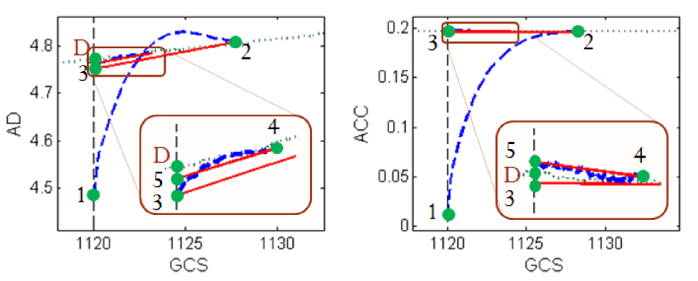
We implement such a lifting operation beginning with a network that possesses the required value of giant component size, by creating an Erdös-Rényi random graph whose number of nodes is equal to the size of the giant component; we then add nodes of zero degree until the network has the correct number of total nodes. Let us denote this result by point $1$ in Fig. 5. We then run the model for a few (here, typically $70$) time steps and obtain network $2$, which lies close to the slow manifold, but has a different value of GCS than required. We now appropriately add/remove enough nodes from this network $2$ until the resulting network $3$ has the required number of nodes in its giant component. This adjustment step is illustrated as a straight line segment in the schematic, for convenience (we do not control the other variables during the adjustment step). If we add nodes to the giant component, we assign them a degree sampled from the current giant component degree distribution. This can be done by randomly selecting a node in the current giant component and using its degree as the degree of the added node. This node is then connected to as many nodes of the giant component as its degree. If we remove nodes from the giant component, they become isolated nodes of degree $0$. When removing nodes, one must of course be careful not to break up the giant component. This is taken care of by first constructing a spanning tree of the giant component, and only removing the fringe nodes of degree $1$ in this tree. All the edges connected to this node in the original graph are then finally removed. In this paper these lifting steps are repeated two or three times as necessary ($2\rightarrow 3,4\rightarrow 5,\ldots$) so that we obtain a network close to the desired graph $D$ in the schematic. We also show an actual sample graph evolution during our lifting operation in Fig. 6. In this case, the required giant component size is $1120$. We start from an Erdös-Rényi random graph (average degree around $4.5$) and perform two iterations of the lifting operation. As explained earlier, each iteration consists of a process step (dashed, blue line) and an adjustment step (solid, red line). The desired, “lifted” graph is labeled ‘D’; the lifting operator arrives at it through intermediate graphs in the sequence from $1$ to $5$.

Figure 6: Graph evolution during our lifting operation is tracked through plots of average degree (AD) and average clustering coefficient (ACS) versus giant component size (GCS). Here, the required value of giant component size is $1120$. The graph with this desired value of giant component size and on the slow manifold (plotted as thin, dotted green line) is labeled as ‘D’. The lifting operator arrives at it through the intermediate graphs $1$ to $5$, in that order. The dashed (blue) lines denote evolution of the dynamical model: this is the “process step”. The solid (red) lines denote corrections for the change in giant component size: this is the “adjustment step”. The combination of two such steps constitutes a single full iteration. Two such full iterations are shown in this illustration.

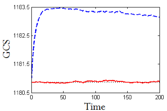
We illustrate the effect of this lifting procedure by evolving the model from two different initial conditions. In the first case, we use a random network created to exhibit the stationary values of the giant component size, the degree distribution and the average clustering coefficient. The evolution of GCS in this case, shown in Fig. 7 as a dashed line (blue), is reminiscent of the left panels of Fig. 4. Thus, it is clear that initializing with the stationary values of GCS, ACC and degree distribution is not sufficient to keep the system close to the slow dynamics; fast transients that take these variables away from their stationary values ensue.

In the second case, we use the lifting procedure just described above to create networks with the stationary GCS value that also are close to the slow manifold. Fig. 7 shows the evolution of the GCS when we run the model starting from these lifted networks as a solid (red) line. Now the giant component size remains close to its stationary value, as desired. This suggests that our lifting procedure is successful.

Figure 7: Trajectories of giant component size observed by simulations from two different classes of initial conditions. The dashed (blue) curve corresponds to the case where the initial condition is a random network created with the stationary values of the giant component size and of the average clustering coefficient as well as the stationary degree distribution. The solid (red) curve corresponds to initial networks created by our lifting procedure, exhibiting the stationary GCS and lying on/close to the slow manifold.

5 Computational results and discussion

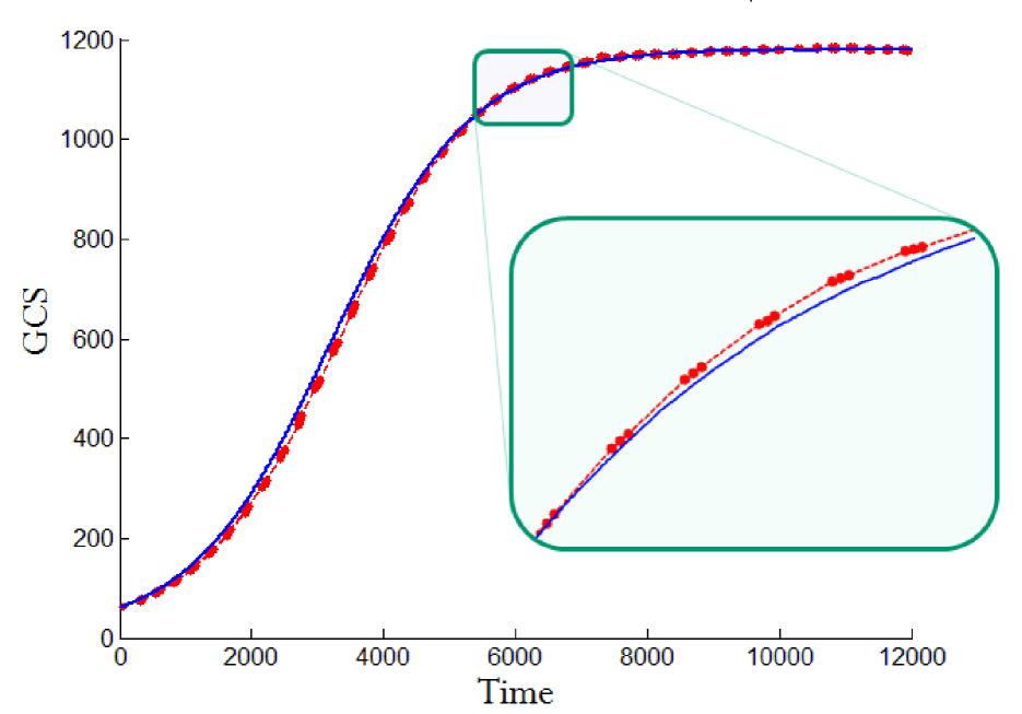
We first validate our coarse-grained modeling by illustrating coarse projective integration of the (expected, averaged over many realizations) system dynamics; we then present coarse bifurcation computations. Let $g$ denote the coarse variable, the giant component size. We start with an ensemble of $2000$ realizations of networks (each with $n=2000$ nodes) exhibiting a specified initial value of this giant component size $g_{0}$. $g$ is evolved using the coarse time-stepper (Eq. 1) for a few (here, 60) time steps. The giant component size is observed from simulations and its time derivative is estimated from the last few time steps of the simulation. This information is used to “project” the coarse variable forward in time through a specified (“long”) time horizon. At the projected time we lift - that is, we construct networks that exhibit the predicted value of giant component size that also lie on the slow manifold as described in the previous section. We used simulation and projection time horizons of $60$ time steps and $210$ time steps, respectively. The time-derivatives required for projection were estimated by using the observed values of giant component size at times $50$ and $60$ of the current simulation step. We show a trajectory computed through coarse projective integration in the left plot of Figure 8 as a dotted (red) line. The data points corresponding to the simulation times are marked as filled (red) circles. The trajectory from full direct simulation is plotted as a solid (blue) line for comparison. It is clear that the two evolutions are visually comparable; yet the projective computation only necessitated simulations for $\frac{60}{270}=22.2\%$, roughly one-fifth of the time. These savings came because of the slow evolution of the (expected value of the) coarse variable, as constrasted to the fast, stochastic (binary - no smooth time derivatives!) evolution of the individual realization fine scale variables. The actual computational savings should also take into account the cost of repeated lifting operations (here, the actual composite computational savings were at $35\%$).

Figure 8: Coarse projective integration of the network evolution, shown by the dotted (red) line, is performed by running direct simulations for $60$ time steps and then projecting forward by $210$ time steps, lifting, and then repeating the procedure. The circle markers correspond to portions of time when the system is actually evolved using fine scale direct simulations. Full direct simulations are also shown as a solid (blue) line for comparison.

Figure 9: Bifurcation diagrams obtained by coarse fixed point computations. Steady state values of average degree, average clustering coefficient and giant component size are plotted against the ratio of parameters, $\xi/\lambda$. The stable branches are plotted as solid (blue) lines, while the unstable branches are plotted as dotted (red) lines. $\eta$ and $\lambda$ values were fixed at $0.001$ and $0.1$ respectively.

Next, we find the coarse steady state of the process time-stepper by solving the following equation (as opposed to finding it by simply evolving the model in time):

$$F(g)=g-\Phi_{60}(g).$$ (2)

This procedure has the advantage of being able to find stable as well as unstable steady states; the latter cannot be found using simple direct simulation. The coarse steady solution, $g_{s}$, to Eq. 2 can be found via a Newton-Raphson procedure. The Jacobian (derivative of $F(g)$ with respect to $g$) required to perform each Newton-Raphson iteration is estimated numerically by evaluating F at neighboring values of $g$. Since this problem involves a single coarse variable, the linearization consists of a single element, that is easy to estimate through numerical derivatives. For problems with large numbers of coarse variables estimating the many components of the linearizations becomes cumbersome, and methods of matrix-free iterative linear algebra (like GMRES as part of a Newton-Krylov GMRES, [17]) become the required tools.

We compute the coarse steady states over a range of parameter values, corresponding to the bifurcation diagram shown in Figure 1. We also keep track of complete network structures corresponding to the coarse steady states on the different solution branches, and store information about steady state values of average degree and average clustering coefficient also. Views of the bifurcation diagram thus produced are shown in the right panels of Figure 8. The bifurcation results qualitatively (and visually quantitatively) agree with those obtained in [1] as reproduced in Figure 1; unstable branches of the bifurcation diagram have now been recovered, and the instabilities (the boundaries of hysteresis) are confirmed (as expected) to be coarse saddle-node bifurcations.

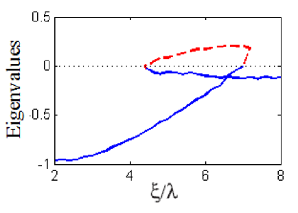
In addition to the steady states, the eigenvalues of the linearization of the coarse time-stepper with respect to the coarse variable (the giant component size) were also estimated at the located steady states. These eigenvalues, which give quantitative information about the stability of the different bifurcation branches, are plotted in Fig. 10. The portion of the curve above the x-axis corresponds to the middle branch in the bifurcation diagrams of Fig. 8. Thus, the upper and lower branches in the bifurcation are found out to be stable branches, while the middle branch is unstable as anticipated. Increased noise in the simulations close to the right turning point renders the diagram there slightly imperfect. Once again, the problem has a single-component linearization, which upon convergence of the Newton iteration also constitutes an estimate of the relevant eigenvalue. More generally, matrix-free Krylov-based Arnoldi methods must be used for the estimation of the leading coarse eigenvalues (see e.g. [18] and [19]).

Figure 10: Eigenvalues of the linearization of the coarse time-stepper with respect to the coarse variable (the giant component size). The portion of the curve above the x-axis corresponds to the unstable middle branch (red, dotted lines) in the bifurcation diagrams of Fig. 8. The stable branches are plotted as solid (blue) lines.

6 Conclusions

In this work we have presented a computer-assisted framework for the systematic coarse-graining of the dynamics of evolutionary network problems. For illustration purposes, we used a simple model (introduced by Marsili et al. in [1]), which nevertheless results in the emergence of complex dynamics at the coarse-grained level, including multiplicity of coarse-grained stationary states. The analysis is relatively simple, yet it demonstrates the algorithmic tasks that one can attempt using the proposed approach. Coarse projective integration, that is, acceleration of the detailed evolutionary network model dynamics, as well as coarse fixed point and coarse stability computations can now be performed using the detailed evolutionary network model as a black box simulator. This is accomplished by circumventing the need for obtaining explicit, closed-form macroscopic analytical approximations, effectively providing computer-assisted “on-demand” model reduction. The key assumption here is that evolutionary equations at the macroscopic level can, in principle be obtained, but the required closures are not available due to the complexity of the underlying fine scale dynamics.

The illustrative model also serves to highlight some important issues that arise in this new context of adapting our coarse-graining framework to problems involving complex network dynamics. The selection of good coarse variables is always an important and often a challenging step. For this illustrative model, we established through numerical experimentation that the giant component size is a good coarse variable to capture the slow dynamics, as other network statistics have predominantly fast dynamics and get quickly slaved to the slow dynamics. We also created a procedure for initializing networks (our lifting ) consistent with slow dynamics. By computationally implementing our model reduction, we recovered the entire bifurcation diagram with this one coarse variable, which suggests that this effective one-dimensionality holds over the entire parameter range we have studied. We should add that, within the equation-free framework, there is a number of additional tasks that can in principle be performed, such as the implementation of algorithms that converge on, and continue, higher codimension bifurcation loci, or also algorithms that design stabilizing controllers for unstable coarse stationary states (see e.g. [20]).

For many problems of interest, the selection of the coarse-grained statistics is often done in an ad hoc manner, or is based on intuition. Here we demonstrated the use of simple dynamics arguments and computations to suggest “good” coarse-grained observables, that are subsequently used in equation-free computation. For more complex problems, where the appropriate observables for the coarse-grained description of the system’s behavior may be unknown, the coupling of the equation-free approach with nonlinear data mining approaches such as Diffusion Maps [21, 22] appears to be a promising research direction. This would require the definition of a useful metric quantifying the distance between nearby graphs (see e.g. [23, 24]).

The computations in this paper were relatively simple, since the coarse description consisted of a single scalar variable. For problems where the coarse variables are many (e.g. for problems where a discretized coarse PDE must be solved), it is important to note that one does not need to explicitly estimate each term in large Jacobian matrices. Matrix-free methods (like Newton-Krylov GMRES) [25, 17] can be and have been used for the equation-free, time-stepper based solution of large scale coarse bifurcation problems [19]. In our discussions of coarse projective integration we demonstrated a tangible acceleration of the temporal simulation of network evolution.

The computational savings from equation-free methods are obviously very problem-dependent; for some problems simple direct simulation may be the easiest way to arrive at, say, a stable stationary state, rather than employing the equation-free machinery with its associated computational overhead. There exist, however, tasks such as the location of unstable stationary states, or the continuation of codimension one and higher bifurcations that would simply be impossible through direct simulation, yet become accessible through our framework. As a simple rule of thumb, problems in which there exists a large separation of time scales between the (slow) evolution of the coarse network evolution and the (fast) node-level dynamics probably present the greatest potential for computational savings. It is, of course, important to also note that, if one is capable of analytically deriving accurate coarse-grained approximations, the computational savings would be so dramatic as to obviate the simulations with the detailed model - equation free computations are precisely intended for situations in which coarse-grained equations are assumed to exist, but it is not possible to derive them in closed form.

Finally, the crux of the success of the approach lies almost invariably in the construction of an efficient lifting algorithm - a step conceptually easy to describe, but often problem dependent and very challenging in itself. In the case of coarse-graining network dynamics, the problem of constructing networks with prescribed combinations of statistics is a notoriously difficult one, itself the subject of intense research [26, 27, 28, 29, 30, 31, 32, 33, 34]. Given the interdependence of various network statistical properties, it is also important to be able to efficiently test the graphicality of a given “prescription” - is a network with the prescribed set of statistics even feasible? We have made this graphicality assumption every time we lifted in our paper because of the simplicity of our single coarse variable; yet this is a nontrivial problem when the coarse variables are more, and interdependent. In this context, we would also like to mention the systematic, integer linear programming based approach of [35]. Clearly, algorithms capable of generating graphs with prescribed properties can be naturally integrated in the lifting step of the equation-free framework.

Appendix A A simple singularly-perturbed system of ODEs

Figure 11: A simple singularly perturbed dynamical system is used to illustrate the notion of “pure” slow variables. Top-left: Sample trajectory of the dynamical system comprised of Eq. 3 and Eq. 4 starting from an initial condition $(x,y)=(0,2)$. Bottom-left: The same trajectory is plotted in terms of coordinates $u=(y+x)/2$ and $v=(y-x)/2$. In both plots on the left, the slow manifold is shown as a dotted (red) line. Right: Time series of $x$, $y$, $u$ and $v$ are shown on the right. The label $t$ stands for time. Notice how in the top case ($x$ is “pure slow”) a short simulation brings the trajectory to the slow manifold without practically changing the initial value of $x$. In the bottom case ($u$ is not “pure slow”) the short transient again brings the trajectory to the slow manifold, but away from the initial value of $u$ (see also the text).

Let us consider a simple example of a singularly perturbed system of ordinary differential equations for illustrative purposes:

$$\frac{dx}{dt}=2-x-y,$$ (3)

$$\frac{dy}{dt}=50(\sqrt{x}-y).$$ (4)

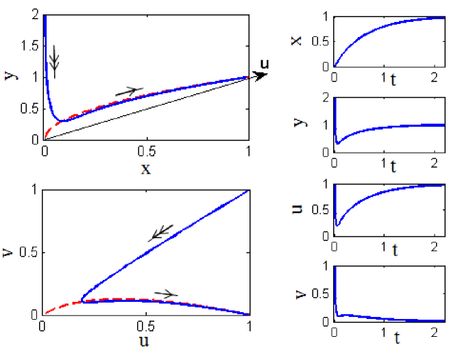
The top left panel of Fig. 11 shows a solution trajectory of this set of equations starting from the initial condition $(x,y)=(0,2)$ as a solid (blue) line. The slow manifold of this set of equations, represented by the curve $y=\sqrt{x}$ is plotted as a dotted (red) line. The trajectories of $x$ and $y$ plotted on the right show that $x$ initially evolves very slowly in time (almost not at all), while $y$ has a fast transient approaching the slow manifold, followed by a slow evolution. It is thus clear from the equations and these figures that $x$ is both a good parameterization of the slow manifold (a good coarse variable) and, at the same time, it is the actual slow variable of the system: a “pure” slow variable.

Consider now the same dynamical system, but with a change of coordinates. Let the new coordinate system be defined by the variables, $u=(y+x)/2$ and $v=(y-x)/2$. The coordinate $u$ is shown as a slanted arrow in the top left plot of Fig. 11. It is clear that the variable $u$ is also (similar to $x$) one-to-one with the slow manifold and hence a suitable candidate for its parameterization, a “good” coarse variable. The solution trajectory computed earlier from the initial condition $(x,y)=(0,2)$ or $(u,v)=(1,1)$ is plotted in terms of coordinates $u$ and $v$ in the lower-left plot of Fig. 11. The corresponding time series of $u$ and $v$ are plotted to the right. The system again evolves quickly to the slow manifold, but $u$ changes quickly in the initial fast transient, away from its initial value. $u$ has thus both fast and slow components - it is not a pure slow variable – even though it can be used to parameterize the slow manifold. Additional effort –more than just a few integration steps– needs to be invested in finding points that have the initial value of $u$ and lie close to/on the slow manifold.

From these figures, it is clear that the direction of fast evolution of the system ($y$ in the original coordinate system, $(u+v)/2$ in the new coordinate system) has a component along the $u$ coordinate. Hence, $u$ is not a pure slow variable, but still a good candidate variable to parameterize the slow manifold: a good coarse variable.

References

- [1] Marsili M, Vega-Redondo F and Slanina F 2004 Proc. Natl. Acad. Sci. 101 1439
- [2] Erdös P and Rényi A 1959 Publicationes Mathematicae (Debrecen) 6 290
- [3] Faloutsos M, Faloutsos P and Faloutsos C 1999 ACM SIGCOMM Comput. Commun. Rev. 29 251
- [4] Yook S-H, Jeong H and Barabási A-L 2002 Proc. Natl. Acad. Sci. 99 13382
- [5] Watts D J and Strogatz S H 1998 Nature 393 440
- [6] Barabási A L and Albert R 1999 Science 286 509
- [7] Davidsen J, Ebel H and Bornholdt S 2002 Phys. Rev. Lett. 88 128701
- [8] Kumpula J M, Onnela J-P, Saramäki J, Kaski K and Kertész J 2007 Phys. Rev. Lett. 99 228701
- [9] Gross T and Kevrekidis I G 2008 Europhys. Lett. 82 38004
- [10] Zschaler G, Traulsen A and Gross T 2010 New J. Phys. 12 093015
- [11] Huepe C, Zschaler G, Do A-L and Gross T 2011 New J. Phys. 13 073022
- [12] Kevrekidis I G, Gear C W, Hyman J M, Kevrekidis P G, Runborg O and Theodoropoulos C 2003 Commun. Math. Sci. 1 715
- [13] Kevrekidis I G, Gear C W and Hummer G 2004 AIChE Journal 50 1346
- [14] Lorenz 1986 J. Atmos. Sci. 43 1547
- [15] Gear C W and Kevrekidis I G 2005 J. Sci. Comp. 25 17
- [16] Zagaris A, Vadekerckhove C, Gear C W, Kaper T J and Kevrekidis I G 2012 Disc. Cont. Dyn. Syst. 32 2759
- [17] Kelley C T 1995 Iterative Methods for Linear and Nonlinear Equations (number 16 in Frontiers in Applied Mathematics, SIAM, Philadelphia, PA)
- [18] Anderson E, Bai Z, Bischof C, Blackford S, Demmel J, Dongarra J, Croz J D, Greenbaum A, Hammarling S, McKenney A and Sorensen D 1999 LAPACK Users’ Guide (Society for Industrial and Applied Mathematics, Philadelphia, PA)
- [19] Siettos C I, Pantelides C C and Kevrekidis I G 2003 Ind. Eng. Chem. Research 42 6795
- [20] Siettos C I, Armaou A, Makeev A G and Kevrekidis I G 2003 AIChE J. 49 1922
- [21] Nadler B, Lafon S, Coifman R R and Kevrekidis I G 2006 Appl. Comput. Harmon. A. 21 113
- [22] Lafon S and Lee A B 2006 IEEE T. Pattern Anal. 28 1393
- [23] Borgs C, Chayes J, Lovász L, Sós V and Vesztergombi K 2006 Topics in Discrete Mathematics: Algorithms and Combinatorics (Springer, Berlin)
- [24] Vishwanathan S V N, Borgwardt K M, Risi Kondor, I and Schraudolph, N N ArXiv e-prints: 0807.0093
- [25] Saad Y and Schultz M H 1986 SIAM J. Sci. Stat. Comp. 7 856
- [26] Havel V 1955 Casopis Pest. Mat. 80 477
- [27] Dorogovtsev S N and Mendes J F F 2001 Phys. Rev. E 63 056125
- [28] Chung F and Lu L 2002 Ann. Comb. 6 125
- [29] Holme P and Kim B J 2002 Phys. Rev. E 65 026107
- [30] Klemm K and Eguíluz V M 2002 Phys. Rev. E 65 057102
- [31] Maslov S and Sneppen K 2002 Science 296 910
- [32] Volz E 2004 Phys. Rev. E 70 056115
- [33] Serrano M A and Boguñá M 2005 Phys. Rev. E 72 036133
- [34] Leary C C, Schwehm M, Eichner M and Duerr H P 2007 Physica A 382 731
- [35] Gounaris C, Rajendran K, Kevrekidis I and Floudas C 2011 Optim. Lett. 5 435