Multiscale reaction-diffusion algorithms:
PDE-assisted Brownian dynamics

Abstract

Two algorithms that combine Brownian dynamics (BD) simulations with mean-field partial differential equations (PDEs) are presented. This PDE-assisted Brownian dynamics (PBD) methodology provides exact particle tracking data in parts of the domain, whilst making use of a mean-field reaction-diffusion PDE description elsewhere. The first PBD algorithm couples BD simulations with PDEs by randomly creating new particles close to the interface which partitions the domain and by reincorporating particles into the continuum PDE-description when they cross the interface. The second PBD algorithm introduces an overlap region, where both descriptions exist in parallel. It is shown that to accurately compute variances using the PBD simulation requires the overlap region. Advantages of both PBD approaches are discussed and illustrative numerical examples are presented.

1 Introduction

Spatial reaction-diffusion models have been widely used for the description of biological systems [25]. Often continuum approaches, written in the form of reaction-diffusion partial differential equations (PDEs), are used due to their simplicity and the vast number of ready-to-use numerical solvers. However, many biological effects cannot be fully described by deterministic PDE-based models. This is because a deterministic model requires large copy numbers of molecules to minimize the relative fluctuation of the spatial concentration. If low copy numbers are present in a biological system [22, 26], then stochastic models such as mesoscopic compartment-based algorithms [19, 6] or trajectory tracking (Brownian dynamics) methods, may be deployed [2, 29].

In many situations individual trajectories are important only in certain parts of the domain, whilst in the remainder of the domain a coarser, less detailed, method can be used [15]. This is the case, for example, in the modelling of ion-channels [24]. Ions pass through a channel in single file and an individual-based model has to be used to accurately compute the discrete, stochastic, current in the channel [4]. The positions of individual ions are less important away from the channel where copy numbers may be very large (rendering a detailed Brownian dynamics description infeasible) [5]. Another example is the stochastic reaction-diffusion modelling of filopodia which are dynamic finger-like protrusions used by eukaryotic motile cells to probe their environment and help guide cell motility [33]. These relatively small protrusions are connected to a larger cytosol compartment. If a modeller is interested to understand the dynamics of filopodia, then there is a potential to decrease the computational cost of simulations by using a coarser model in the cytosol. In both examples, it is important to understand how models with a different level of detail can be used in different parts of the computational domain [15].

In this paper, we develop algorithms that calculate Brownian dynamics (BD) paths in a desired part of the domain, whilst using a continuum PDE-based model in the remainder. This PDE-assisted Brownian dynamics (PBD) methodology has the advantage that efficient methods for solving PDEs can be used for large parts of the modelled domain, whilst BD data is available in other areas where required. The main goal of the PBD methodology is to get the same statistics (means and variances) in the BD subdomain as we would get if we we were able to use BD simulations in the whole domain. In particular, the correct coupling between the two parts of the domain is of vital importance for the accuracy of a PBD algorithm.

The paper is organised as follows. Section 2 states, in mathematical terms, the requirements for the developed algorithms and introduces the notation used throughout the remainder of the paper. We then introduce the first PBD algorithm for a pure diffusion system in Section 3, where we also explore the complications of this algorithm. In Section 4 we present the second PBD algorithm which provides more accurate computations. In Section 5 we investigate issues relating to the introduction of reactions into the system and present several computational examples.

2 Problem formulation

Consider a general Brownian dynamics reaction-diffusion simulation with $M$ chemical species in the (open) domain $\Omega\subset{\mathbb{R}}^{3}$. We denote by $n_{j}(\mathbf{x},t)$, $j=1,2,\dots,M,$ the expected spatio-temporal concentration of the $j$-th chemical species at the position $\mathbf{x}$ and time $t$ over our domain $\Omega$. The approximate mean-field reaction-diffusion PDEs for the time evolution of concentrations can be written as follows

$$\frac{\partial p_{j}}{\partial t}=D_{j}\,\Delta p_{j}+R_{j}(p_{1},p_{2},\dots,p_{M})\,,\qquad j=1,2,\dots,M,$$ (1)

where $p_{j}\equiv p_{j}(\mathbf{x},t):\Omega\times[0,\infty)\to[0,\infty)$ is the mean-field approximation of $n_{j}$, $D_{j}$ is the diffusion constant of the $j$-th chemical species and $R_{j}:[0,\infty)^{M}\to{\mathbb{R}}$ represents the reaction terms.

The goal of PBD algorithms is to couple macroscopic description (1) in the open subdomain $\Omega_{P}\subset\Omega$ with a stochastic BD simulation in the open subdomain $\Omega_{B}\subset\Omega$, where the closures of $\Omega_{B}$ and $\Omega_{P}$ cover $\Omega$, i.e.

$$\Omega\subset\overline{\Omega_{B}}\cup\overline{\Omega_{P}}.$$ (2)

In $\Omega_{B}$, we will consider BD trajectories of individual molecules, i.e. the state of the microscopic subdomain $\Omega_{B}$ is defined by the number $N_{B}^{(j)}(t)$ of molecules of the $j$-th chemical species at time $t$ and their positions ${\mathbf{x}}_{i}^{(j)}(t)\in\Omega_{B}$, $i=1,2,\dots,N_{B}^{(j)}(t)$, $j=1,2,\dots,M$. We denote by $I$ the interface between the subdomains $\Omega_{B}$ and $\Omega_{P}$, namely

$$I=\overline{\Omega_{B}}\cap\overline{\Omega_{P}}.$$ (3)

In this paper, we will investigate two cases:

[A] $\Omega_{B}$ and $\Omega_{P}$ do not overlap, i.e. $\Omega_{B}\cap\Omega_{P}=\emptyset$;

[B] there exists an overlap region where the PDE description and BD simulations exist in parallel, i.e. $\Omega_{B}\cap\Omega_{P}\not=\emptyset.$

The case [A] will lead to the PBD algorithm (A1)–(A5) presented in Table 1. The case [B] is implemented in the second PBD algorithm (B1)–(B5) which is presented in Table 2. We will start our discussion with the case [A] because it is less technical to implement than the case [B].

To simplify our presentation, we will consider that $\Omega$ is a “narrow” three-dimensional domain, and hence only consider the process mapped onto an effective one-dimensional domain $\Omega\subset\mathbb{R}$ by assuming that the system is well mixed in the other two dimensions. In particular, we have $\Omega_{B}\subset\Omega\subset\mathbb{R}$ and the state of the BD subdomain $\Omega_{B}$ will be described by the $x$-coordinates of molecules which we will denote as $x_{i}^{(j)}(t)\in\Omega_{B}$, $i=1,2,\dots,N_{B}^{(j)}(t)$, $j=1,2,\dots,M$. We simulate the system using finite time step $\Delta t>0$, in which particles in $\Omega_{B}$ change their position according to the discretized version of the overdamped Langevin equation

$$x_{i}^{(j)}(t+\Delta t)=x_{i}^{(j)}(t)+\sqrt{2D_{j}\Delta t}\,\xi\,,$$ (4)

where $\xi$ is a normally distributed random variable with zero mean and unit variance. Figure 1 shows a sketch of the described system for one chemical species along with the notation used in the case [A].

\begin{overpic}[width=260.17464pt]{./Figure2_1} \put(20.0,2.0){\Large$\Omega_{P}$} \put(70.0,2.0){\Large$\Omega_{B}$} \put(51.0,2.0){\Large$I$} \put(20.0,45.0){\color[rgb]{0,0,1}\Large$p(x,t)$} \put(70.0,45.0){\Large$N_{B}(t)$} \put(60.0,34.0){\color[rgb]{0.13,0.55,0.13}\large$x_{1}(t)$} \put(80.0,34.0){\color[rgb]{0.13,0.55,0.13}\large$x_{i}(t)$} \put(94.0,20.0){\large$t$} \put(50.0,-5.0){\Large$x$} \end{overpic}

Fig. 1: Sketch of the first PBD algorithm and the notation related to it. In $\Omega_{P}$, molecules are described by their density distribution $p(x,t)$ and in the microscopic domain $\Omega_{B}$ described by the number $N_{B}(t)$ of molecules and their positions $x_{i}(t)$, $i=1,2,\dots,N_{B}(t)$. The interface between these domains is denoted $I$.

Our goal is to construct PBD algorithms which will satisfy the following two conditions:

Condition (C.1): We require that the expected distribution of molecules in $\Omega_{B}\setminus\Omega_{P}$ match that of the expected distribution $n_{j}(x,t)$, i.e. the distribution which we would obtain if we used detailed BD simulations in the whole domain $\Omega$. In particular this means that for every set $A\subset\Omega_{B}\setminus\Omega_{P}$, the expected number of particles in $A$ at time $t>0$ has to satisfy

$$\mathbb{E}\left[\left|\left\{x_{i}^{(j)}(t)\in A\;,i=1,\ldots,N_{B}^{(j)}(t)\right\}\right|\right]=\int_{A}n_{j}(x,t)\mathrm{d}x\,,\qquad\forall A\subset\Omega_{B}\setminus\Omega_{P}\,.$$ (5)

The choice of an arbitrarily small but finite interval $A=[x,x+\mathrm{d}x)$ for $x\in\Omega_{B}\setminus\Omega_{P}$ leads to an alternative formulation of this condition

$$\mathbb{E}\left[\left|\left\{x_{i}^{(j)}(t)\in[x,x+\mathrm{d}x)\;,i=1,\ldots,N_{B}^{(j)}(t)\right\}\right|\right]=n_{j}(x,t)\mathrm{d}x\,,\qquad\forall x\in\Omega_{B}\setminus\Omega_{P}\,.$$ (6)

Condition (C.2): Whilst we aim to match the expected outcome of the stochastic simulation to $n(x,t)$, we also want the variances of molecule distribution in $\Omega_{B}\setminus\Omega_{P}$ to match that which would be expected if a BD simulation were to be performed over the entire domain $\Omega$.

In $\Omega_{P}\setminus\Omega_{B}$, the system is described by the concentration vector $p_{j}$, $j=1,2,\dots,M$, which evolves according to the PDE (1). This distribution, whilst continuous, is not strictly deterministic since it is coupled with the stochastic outcomes of the BD subdomain $\Omega_{B}$. If the stochastic reaction-diffusion model only includes zero-order or first-order reactions, then the mean-field PDE (1) describes the expected behaviour of stochastic models [12]. In this case it is reasonable to require the following additional condition.

Condition (C.3): We require

$$\mathbb{E}\left[p_{j}(x,t)\right]=n_{j}(x,t)\,,\qquad\forall x\in\Omega_{P}\setminus\Omega_{B}\,,\ t>0\,.$$ (7)

In the case [A], the conditions (C.1)–(C.3) can be simplified by observing that $\Omega_{B}=\Omega_{B}\setminus\Omega_{P}$ and $\Omega_{P}=\Omega_{P}\setminus\Omega_{B}$. In the case [B], we will also require that the PBD algorithm gives the correct mean distribution of molecules in the overlap region $O=\Omega_{B}\cap\Omega_{P}$, i.e.

$$\mathbb{E}\left[p_{j}(x,t)\right]\mathrm{d}x+\mathbb{E}\left[\left|\left\{x_{i}^{(j)}(t)\in[x,x+\mathrm{d}x)\;,i=1,\ldots,N_{B}^{(j)}(t)\right\}\right|\right]=n_{j}(x,t)\mathrm{d}x$$ (8)

for all $x\in O=\Omega_{B}\cap\Omega_{P}$ and $t>0.$

3 PBD simulation of diffusion

In this section, we explain our case [A] PBD algorithm (i.e. $\Omega_{B}\cap\Omega_{P}=\emptyset$) using a system of diffusing non-interacting molecules of a single chemical species. Therefore, for all further discussions in this and the following section we will drop the index $j$ representing the species. Then the macroscopic PDE (1) for this system becomes the diffusion equation

$$\frac{\partial n}{\partial t}=D\frac{\partial^{2}n}{\partial x^{2}}\,,$$ (9)

where $n\equiv n(x,t):\Omega\times[0,\infty)\to[0,\infty)$ and $D$ is the diffusion constant. We will consider the infinite domain $\Omega=\mathbb{R}$ for simplicity. Without loss of generality, we assume that $\Omega_{P}=(-\infty,0)$ and $\Omega_{B}=(0,\infty)$, i.e. the internal boundary $I=\{0\}$ is situated at the origin $x=0$. In the case of diffusion only, the total number of molecules $N$ in the system is conserved, i.e.

$$N=\int_{\Omega}n(x,t)\,\mathrm{d}x,\qquad\mbox{for all}\;t\geq 0\,.$$ (10)

Hence, for the PBD algorithm the conservation of mass condition takes the form

$$N=\int_{\Omega_{P}}p(x,t)\,\mathrm{d}x+N_{B}(t)\,,\qquad\mbox{for all}\;t\geq 0\,.$$ (11)

Since the diffusing molecules are non-interacting, we can express Condition (C.2) in mathematical terms. If all particles start with the same initial condition, then each particle has the (identical) probability $p_{A}=\int_{A}n(x,t)\mathrm{d}x/N$ of being in a set $A$ at time $t$. Consequently, the expected number of particles in $A$ at time $t$ is $Np_{A}$ and the variance is equal to $Np_{A}(1-p_{A})$. Substituting $p_{A}=\int_{A}n(x,t)\mathrm{d}x/N$ and using (10), we get Condition (C.2) in the following form

$$\operatorname{var}\left[\left|\left\{x_{i}(t)\in A\;,i=1,\ldots,N_{B}(t)\right\}\right|\right]=\int_{A}n(x,t)\mathrm{d}x\left(1-\frac{\int_{A}n(x,t)\mathrm{d}x}{\int_{\Omega}n(x,t)\mathrm{d}x}\right)\,,$$ (12)

for all $A\subset\Omega_{B}$ and $t>0$. Using again $A=[x,x+\mathrm{d}x)$, we obtain the alternative formulation

$$\operatorname{var}\left[\left|\left\{x_{i}(t)\in[x,x+\mathrm{d}x)\;,i=1,\ldots,N_{B}(t)\right\}\right|\right]=n(x,t)\mathrm{d}x\,.$$ (13)

In Sections 3.1 and 3.2, we present one update step of the continuum and the particle-based simulations respectively, before the full PBD algorithm (A1)–(A5) is formulated in Section 3.3. In Section 3.4, we will discuss the accuracy of the algorithm with respect to the Conditions (C.1)–(C.3).

3.1 Updating the PDE regime in $\Omega_{P}$

At time $t$, we have the concentration $p(x,t)$ for $x\in\Omega_{P}$ and are aiming to calculate the concentration $p(x,t+\Delta t)$ that corresponds to a realisation of one time step $\Delta t$ of the diffusion process (9). We therefore define the exact outcome of a diffusion step in the full domain $\Omega$ given initial data $p(x,t)$:

$$\widetilde{p}(x,t+\Delta t)=\int_{\Omega_{P}}K(x-x^{\prime},\Delta t)\,p(x^{\prime},t)\,\mathrm{d}x^{\prime}\,,$$ (14)

where $K(x-x^{\prime},\Delta t)$ is the diffusion kernel

$$K(\xi,\Delta t)=\frac{1}{\sqrt{4\pi D\Delta t}}\exp\left(-\frac{\xi^{2}}{4D\Delta t}\right)\,,$$ (15)

and the function $\widetilde{p}(x,t)$ has support $\Omega$. Using this process, a certain proportion of the concentration distribution, namely

$$\alpha(t+\Delta t)\equiv\int_{\Omega_{B}}\widetilde{p}(x,t+\Delta t)\,\mathrm{d}x$$ (16)

would have crossed the interface $I$ in the time interval $[t,t+\Delta t)$ (see Figure 2).

\begin{overpic}[width=260.17464pt]{./Figure3_1} \put(30.0,2.0){\Large$\Omega_{P}$} \put(85.0,2.0){\Large$\Omega_{B}$} \put(62.0,2.0){\Large$I$} \put(25.0,45.0){\color[rgb]{0.6,0.6,0.6}\Large$p(x,t)$} \put(25.0,35.0){\Large$\widetilde{p}(x,t+\Delta t)$} \put(70.0,10.0){\color[rgb]{0.75,0.19,0.38}\Large$\alpha(t+\Delta t)$} \put(50.0,-5.0){\Large$x$} \end{overpic}

Fig. 2: Illustration of step (A1) of the first PBD algorithm. Dashed line: $p(x,t)$; solid line: $\widetilde{p}(x,t+\Delta t)$ as defined in (14); shaded area: $\alpha(t+\Delta t)$ as defined in (16).

This value $\alpha(t+\Delta t)$ represents the expected number of molecules to cross the interface from $\Omega_{P}$ to $\Omega_{B}$ in the time interval $[t,t+\Delta t)$. Since all molecules in $\Omega_{P}$ are identical (of the same chemical species and have the same probability distribution proportional to $\widetilde{p}(x,t+\Delta t)$), the number of molecules that cross the interface from $\Omega_{P}$ to $\Omega_{B}$ in the time interval $[t,t+\Delta t)$ is Poisson distributed with average $\alpha(t+\Delta t)$. Let us assume that $\Delta t$ has been chosen small enough to ensure that $\alpha(t+\Delta t)\ll 1$. In this case the probability of more than one particle crossing the interface is negligible and we need to consider two cases:

(i) one particle gets created in $\Omega_{B}$ with the probability $\alpha(t+\Delta t)$;

(ii) no particle is created with the probability $1-\alpha(t+\Delta t)$.

For both cases we need to calculate the updated concentration $p(x,t+\Delta t)$ where $x\in\Omega_{P}$.

We consider the concentration $p(x,t)$ as the distribution of $N-N_{B}(t)$ identically distributed particles at time $t$. Therefore each of these particles has at time $t$ the probability distribution $p(x,t)/(N-N_{B}(t))$. After one time step each of these particles can be found in an infinitesimal interval $[x,x+\mathrm{d}x)$ with probability $\widetilde{p}(x,t+\Delta t)\,\mathrm{d}x$. For each particle, its probability distribution given that it did not leave $\Omega_{P}$ can be calculated as

$$p_{1}(x,t+\Delta t)=\frac{\widetilde{p}(x,t+\Delta t)}{N-N_{B}(t)-\alpha(t+\Delta t)}\,,\qquad\mbox{for}\;x\in\Omega_{P}\,.$$

On the other hand, if a particle does leave the domain $\Omega_{P}$, then its distribution function becomes zero for $x\in\Omega_{P}$. Instead the particle is introduced into $\Omega_{B}$ at time $t+\Delta t$ at a location $x$ with the probability distribution given by

$$p_{2}(x,t+\Delta t)=\frac{\widetilde{p}(x,t+\Delta t)}{\alpha(t+\Delta t)}\,,\qquad\mbox{for}\;x\in\Omega_{B}\,.$$ (17)

This updating process is rather like collapsing a wavefunction in quantum mechanics [30]. We have a look to see if a particle has crossed the boundary into $\Omega_{B}$: if it is there on the other side then its distribution function collapses to a $\delta$ function at its new position, while if it is not, then the distribution function collapses to zero in $\Omega_{B}$ with corresponding rescaling in $\Omega_{P}$.

Combining these arguments for all the particles, we see that the last update step is a simple rescaling of the probability distribution so that the updated distribution satisfies conservation of mass according to (11). We therefore have

$$p_{\mathrm{cont}}(x,t+\Delta t)=\left\{\begin{array}[]{ll}\beta_{(i)}\,\widetilde{p}(x,t+\Delta t),&\mbox{in the case (i),}\\ \beta_{(ii)}\,\widetilde{p}(x,t+\Delta t),&\mbox{in the case (ii).}\end{array}\right.\quad\mbox{for}\;x\in\Omega_{P}\,,$$ (18)

with the rescaling constants $\beta_{(i)},$ $\beta_{(ii)}$ given by

$$\beta_{(i)}=\frac{N-N_{B}(t)-1}{N-N_{B}(t)-\alpha(t+\Delta t)}\,,\qquad\beta_{(ii)}=\frac{N-N_{B}(t)}{N-N_{B}(t)-\alpha(t+\Delta t)}\,.$$ (19)

Note that the update step for the continuum regime satisfies conservation of mass (11). An illustration of the two cases can be seen in Figure 3.

\begin{overpic}[width=195.12767pt]{./Figure3_2a} \put(30.0,2.0){$\Omega_{P}$} \put(85.0,2.0){$\Omega_{B}$} \put(62.0,2.0){$I$} \put(50.0,-3.0){$x$} \put(25.0,45.0){\color[rgb]{0.6,0.6,0.6} $\widetilde{p}(x,t+\Delta t)$} \put(25.0,37.0){$p_{\mathrm{cont}}(x,t+\Delta t)$} \put(72.0,14.0){\small\color[rgb]{0.13,0.55,0.13} $x_{i}(t+\Delta t)$} \put(70.0,45.0){$N_{B}(t)+1$} \end{overpic}

(a) Case (i)

\begin{overpic}[width=195.12767pt]{./Figure3_2b} \put(30.0,2.0){$\Omega_{P}$} \put(85.0,2.0){$\Omega_{B}$} \put(62.0,2.0){$I$} \put(50.0,-3.0){$x$} \put(25.0,45.0){\color[rgb]{0.6,0.6,0.6} $\tilde{p}(x,t+\Delta t)$} \put(25.0,37.0){$p_{\mathrm{cont}}(x,t+\Delta t)$} \put(80.0,45.0){$N_{B}(t)$} \end{overpic}

(b) Case (ii)

Fig. 3: Illustration of steps (A2) and (A3) of the first PBD algorithm. Dashed line: $\widetilde{p}(x,t+\Delta t)$; solid line: $p_{\mathrm{cont}}(x,t+\Delta t)$; (green) circle: created particle.

3.2 Updating the BD regime in $\Omega_{B}$

We use the discretized version of the overdamped Langevin equation introduced in (4) to update the positions of particles in $\Omega_{B}$. If the position of the $i$-th molecule, computed by (4), is in $\Omega_{B}$ at the end of the time step, then we will continue representing it as a particle. Note, that a particle that crossed the boundary $I$ and came back into $\Omega_{B}$ during the time step $[t,t+\Delta t)$ is also captured by this case. We have to be more careful whenever the position $x_{i}(t+\Delta t)$, computed by (4), is inside the PDE subdomain $\Omega_{P}$ at time $t+\Delta t$, i.e. $x_{i}(t+\Delta t)\in\Omega_{P}$. In this case, the random walk of the $i$-th molecule crossed the interface $I$ without crossing back at the end of the time step. This event needs to be taken into account for the update of the final concentration $p(x,t+\Delta t)$ in $\Omega_{P}$. As we know the exact position of this particle $i$ at time $t+\Delta t$ we add a Dirac $\delta$ function at the position $x_{i}(t+\Delta t)\in\Omega_{P}$. Therefore we compute $p(x,t+\Delta t)$ in $\Omega_{P}$ by

$$p(x,t+\Delta t)=p_{\mathrm{cont}}(x,t+\Delta t)+\sum_{x_{i}(t+\Delta t)\in\Omega_{P}}\delta(x-x_{i}(t+\Delta t)),$$

where $p_{\mathrm{cont}}(x,t+\Delta t)$ is given by (18).

3.3 The first PBD algorithm

This algorithm computes the concentration $p(x,t)$ for $x\in\Omega_{P}$, and the number $N_{B}(t)$ and positions of BD particles $x_{i}(t)\in\Omega_{B}$, $i=1,2,\dots,N_{B}(t).$ One time step of the first PBD algorithm is presented in Table 1 as algorithm (A1)–(A5). In order to simplify the presentation of this algorithm, we consider that the time step $\Delta t$ is chosen so small that $\alpha(t+\Delta t)\ll 1$. In particular, we only need to implement cases (i)–(ii) presented in Section 3.1, because the probability that two or more molecules are initiated in $\Omega_{B}$ during one time step is negligible.

The auxiliary distribution $\widetilde{p}(x,t+\Delta t)$ in step (A1) is in practice calculated using a numerical approximation algorithm. To calculate $\alpha(t+\Delta t)$ we can either use this numerical approximation of $\,\widetilde{p}(x,t+\Delta t)$, which requires an additional time step $\widetilde{\Delta t}\ll\Delta t$ to be used to ensure the accuracy of $\alpha(t+\Delta t)$, or (more efficiently) we can approximate $\alpha(t+\Delta t)$ analytically using a boundary layer expansion in the vicinity of the interface $I$.

1. Calculate $\widetilde{p}(x,t+\Delta t)$ using (14) and $\alpha(t+\Delta t)$ using (16).

2. Generate uniformly distributed random number $r$ in $(0,1)$.

   1. If $r<\alpha(t+\Delta t)$, then create new particle in $\Omega_{B}$ according to the probability density $p_{2}(x,t+\Delta t)$ defined in (17). Set $\beta=\beta_{(i)}$ where $\beta_{(i)}$ is given by (19). Set $N_{B,1}=1.$

   2. If $r\geq\alpha(t+\Delta t)$, then set $\beta=\beta_{(ii)}$ where $\beta_{(ii)}$ is given by (19).
      Set $N_{B,1}=0.$

3. Compute positions $x_{i}(t+\Delta t)$, $i=1,2,\dots,N_{B}(t)$, of BD particles according to (4).

4. Compute new concentration in $\Omega_{P}$ by

   $$p(x,t+\Delta t)=\beta\,\widetilde{p}(x,t+\Delta t)+\sum_{x_{i}(t+\Delta t)\in\Omega_{P}}\!\!\!\!\!\delta(x-x_{i}(t+\Delta t))\,,\quad\mbox{for}\;x\in\Omega_{P}\,.$$

5. Update the number of BD particles by

   $$N_{B}(t+\Delta t)=N_{B}(t)+N_{B,1}-\left|\left\{x_{i}(t+\Delta t)\in\Omega_{P}\;,i=1,\dots,N_{B}(t)\right\}\right|\,.$$

   Terminate computation of trajectories of BD molecules which landed in $\Omega_{P}$ (i.e. the BD particles which satisfy $x_{i}(t+\Delta t)\in\Omega_{P}.$)
   Then continue with step (A1) for time $t+\Delta t$.

Table 1: One time step of the first PBD algorithm for a system of diffusing molecules.

By construction, the algorithm (A1)–(A5) satisfies the conservation of mass condition (11) and the concentration $p(x,t)$ satisfies non-negativity. We will now show that this algorithm also guarantees the correct expected outcome and therefore satisfies Conditions (C.1) and (C.3).

Theorem 1.

Consider the BD simulation of $N$ diffusing molecules in the computational domain $\Omega$ which is divided into sudomains $\Omega_{B}\subset\Omega$ and $\Omega_{P}\subset\Omega$ satisfying $(\ref{omegacoverage})$ and the case [A]. Suppose that $N_{B}(0)$ particles are initially in $\Omega_{B}$ at positions $x_{i}(0)$, $i=1,2,\dots,N_{B}(0).$ Let us initialize $p(x,0)$ as sums of Dirac $\delta$ functions describing molecules which are initially in $\Omega_{P}$, i.e. $p(x,0)=n(x,0)$ for $x\in\Omega_{P}$. Then the expected outcome of the PBD algorithm (A1)–(A5) (presented in Table 1) satisfies the Conditions (C.1) and (C.3) for arbitrary $\Delta t>0$.

Proof.

We will show that the identities (5) and (7) hold during one iteration (A1)–(A5) presented in Table 1. It will then follow by induction that they hold for all times $k\Delta t$, $k=0,1,2,\dots$.

Let us assume that the probability distribution of particles in $\Omega_{B}$ at time $t$ is given through $n(x,t)$, $x\in\Omega_{B}.$ Given the probability distribution $p(x,t)$, $x\in\Omega_{P}$, at time $t$, the conditional expected value of $p(x,t+\Delta t)$ for $x\in\Omega_{P}$ is given by

$$\mathbb{E}\,\big{[}\,p(x,t+\Delta t)\,|\,p(x,t)\,\big{]} = \alpha(t+\Delta t)\,\beta_{(i)}\,\widetilde{p}(x,t+\Delta t)$$

$$+ (1-\alpha(t+\Delta t))\,\beta_{(ii)}\,\widetilde{p}(x,t+\Delta t)$$

$$+ \int_{\Omega_{B}}K(x-x^{\prime},\Delta t)\,n(x^{\prime},t)\,\mathrm{d}x^{\prime}\,,$$

where $\beta_{(i)}$ and $\beta_{(ii)}$ are given by (19), $K(x-x^{\prime},\Delta t)$ is the diffusion kernel given in (15) and the last term represents particles that moved across the interface $I$, defined by (3), during the time step $[t,t+\Delta t)$. Using (19), we obtain

$$\mathbb{E}\,\big{[}\,p(x,t+\Delta t)\,|\,p(x,t)\,\big{]}=\widetilde{p}(x,t+\Delta t)+\int_{\Omega_{B}}K(x-x^{\prime},\Delta t)\,n(x^{\prime},t)\,\mathrm{d}x^{\prime}.$$

Using (14) and the law of total expectation (law of iterated expectations), we get

$$\mathbb{E}\,\big{[}p(x,t+\Delta t)\,\big{]}=\int_{\Omega_{P}}\!K(x-x^{\prime},\Delta t)\,\mathbb{E}[p(x^{\prime},t)]\,\mathrm{d}x^{\prime}+\int_{\Omega_{B}}\!K(x-x^{\prime},\Delta t)\,n(x^{\prime},t)\,\mathrm{d}x^{\prime}.$$

Using the induction assumption that $\mathbb{E}[p(x,t)]=n(x,t)$, we obtain

$$\mathbb{E}\,\big{[}p(x,t+\Delta t)\,\big{]}=\int_{\Omega}n(x^{\prime},t)K(x-x^{\prime},\Delta t)\,\mathrm{d}x^{\prime}=n(x,t+\Delta t)\,,\quad\mbox{for}\;x\in\Omega_{P}\,,$$

i.e. we have derived (7).

Let us consider a set $A\subset\Omega_{B}$. Given the probability distribution $p(x,t)$, $x\in\Omega_{P}$, at time $t$, the conditional expected number of particles in $A$ at time $t+\Delta t$ is

$$\mathbb{E}\,\big{[}\left|\left\{x_{i}(t)\in A\;,i=1,\ldots,N_{B}(t)\right\}\right|\,\big{|}\,p(x,t)\,\big{]} = \int_{A}\alpha(t+\Delta t)\,p_{2}(x,t+\Delta t)\,\mathrm{d}x$$

$$+ \int_{A}\int_{\Omega_{B}}K(x-x^{\prime},\Delta t)\,n(x^{\prime},t)\,\mathrm{d}x^{\prime}\,\mathrm{d}x,$$

where the first term represents newly created particles from the PDE regime $\Omega_{P}$ and the second term represents the movement of particles inside $\Omega_{B}$. Using (14), (17) and the law of total expectation, we obtain

$$\mathbb{E}\,\big{[}\,\big{|}\,\left\{x_{i}(t)\in A\;,i=1,\ldots,N_{B}(t)\right\}\,\big{|}\,\,\big{]} = \int_{A}\int_{\Omega}K(x-x^{\prime},\Delta t)\,n(x^{\prime},t)\,\mathrm{d}x^{\prime}\,\mathrm{d}x$$

$$= \int_{A}n(x,t+\Delta t)\,\mathrm{d}x\,,$$

which is the condition (5). Thus we have showed that both Conditions (C.1) and (C.3) are satisfied. This concludes the proof. ∎

Theorem 1 also holds if the algorithm (A1)–(A5) is extended to the creation of more than one new particle per time step as long as the expected value of the number of created particles is $\alpha(t+\Delta t)$ and the rescaling is done accordingly. The algorithm (A1)–(A5) and the proof can be easily extended for a finite domain $\Omega=[0,L]$ with no flux boundary conditions by redefining the kernel $K(\xi,\Delta t)$ accordingly.

3.4 Discussion of the PBD algorithm (A1)–(A5)

In Theorem 1 we showed that the PBD algorithm (A1)–(A5) satisfies the Conditions (C.1) and (C.3). However, we still need to check whether the Condition (C.2) on the variances is also satisfied.

To investigate the variances created by this algorithm, we show the outcome of an illustrative numerical example in Figure 4. We simulate the diffusion of 100 molecules in the domain $\Omega=[-1,1]$ which are initialized at the same location $x=-0.95$. We use no flux boundary conditions. We test the algorithm (A1)–(A5) where $\Omega_{P}=(-1,0)$, $\Omega_{B}=(0,1)$ and $I=\{0\}$. To calculate $\widetilde{p}(x,\Delta t)$ we use an implicit Euler-scheme with $\Delta x=0.01$ and a numerical time-step of $\widetilde{\Delta t}=10^{-6}$. The time step $\Delta t$ used by the algorithm (A1)–(A5) is $\Delta t=10^{-3}$ and we simulate the system until $T_{\mathrm{final}}=0.2$. The time step $\widetilde{\Delta t}\ll\Delta t$ for the approximation of $\widetilde{p}(x,t+\Delta t)$ was chosen in order to minimise numerical artefacts. We run 1000 realisations of this process and measured the number of particles in 10 intervals (‘bins’) of the size $0.1$ in $\Omega_{B}$. Averaging over 1000 realisations, we calculate the mean value and the variance of the particle number for each of the bins at time $T_{\mathrm{final}}$. The results are presented in Figure 4 as gray histograms. In this example, it is easy to calculate the correct distribution $n(x,t)$ which the algorithm (A1)–(A5) tries to approximate. It can be obtained by solving the diffusion equation (9) in the domain $\Omega=(-1,1)$ with $n(x,0)=100\,\delta(x+0.95)$ and no flux boundary conditions. The expected values for both means and variances are plotted as (red) dashed lines in Figure 4.

(a) Mean

(b) Variance

Fig. 4: Simulation results of diffusion of 100 particles in $(-1,1)$ with no flux boundary conditions initialized at $x=-0.95,$ i.e. $n(x,0)=100\,\delta(x+0.95)$. Results averaged over 1000 realisations. Dashed (red) line: expected outcome. (a) Solid line: mean value in $\Omega_{P}$; (gray) bars: particle concentrations in $\Omega_{B}$. (b) (Gray) bars: measured variances in particle concentrations. Parameter values are described in the text.

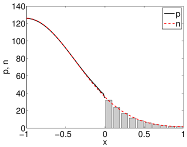
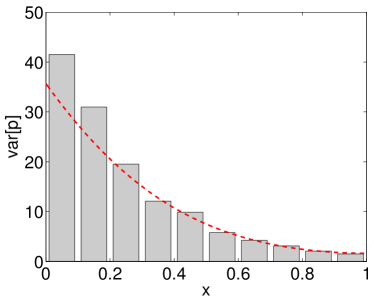
In Figure 4(a), we see that the mean value of the simulation results matches well with the solution of the diffusion process, with only small fluctuations close to the internal boundary $I$ at $x=0$ due to stochastic effects and inaccuracies caused by the numerical approximation of $\widetilde{p}(x,t+\Delta t)$. However, in Figure 4(b) it becomes clear that the variance between different realisations is higher than the desired value, in particular close to the internal interface. We can explain this effect clearly using a thought experiment.

Let us consider a situation where $p(x,0)$ is $0$ close to the internal boundary $I$ and has a peak of mass 99 arbitrarily far away from $I$. Additionally, we assume that one particle is situated in $\Omega_{B}$ close to the interface $I$. Assuming the particle crosses the interface in the first simulation step, a Dirac $\delta$ function is created in $\Omega_{P}$ close to the interface, as illustrated in Figure 5(a). This $\delta$ function has a large impact on the region in $\Omega_{P}$ that is close to the interface, as the distribution $p(x,\Delta t)$ is negligible in this region. Immediately after incorporating the particle into $p(x,\Delta t)$, all its information is lost and we are forced to assume $100$ independent particles with the probability distribution $p(x,\Delta t)$ in $\Omega_{P}$. In particular this implies that every particle has a $1\%$ chance of being at the position of the $\delta$ and $99\%$ chance of being in the bulk distribution far away from the boundary. This is indeed not the case, since we know that there is exactly one molecule near the interface and 99 molecules away from the interface, but the nature of the continuum distribution means that this information must be lost or else we should necessarily demand a separate distribution for all molecules in $\Omega_{P}$.

In the second diffusion step, we calculate $\widetilde{p}(x,2\Delta t)$ according to (14) and some ‘mass’ $\alpha(2\Delta t)$ may have drifted across the interface $I$ (see Figure 5(b)). Because the bulk distribution is far away from the boundary, almost all of this mass $\alpha(2\Delta t)$ comes from the $\delta$ function close to $I$. Let us imagine that a new particle is now created in $\Omega_{B}$ (according to the probability $\alpha(2\Delta t)$), in which case the whole distribution needs to be rescaled, as shown in Figure 5(c). Because $99\%$ of the mass in $p(x,\Delta t)$ is situated in the bulk far away from the boundary, the majority of the rescaling happens in this region, such that effectively the mass needed to create the particle is almost entirely taken from the bulk, rather than from the region close to the interface. This also implies that most of the mass close to the boundary will stay and it is therefore possible to create another particle from this mass in further time steps. This is in contradiction to the result that would be expected if information was not lost in the first time step. That is, the distribution close to the interface should dissapear and the bulk far from the interface is left alone. This effect is the main reason a higher than expected variance can be measured in $\Omega_{B}$. Note, however, that this does not effect the expected values, as shown in Theorem 1.

\begin{overpic}[width=195.12767pt]{./Figure3_4a} \put(30.0,2.0){$\Omega_{P}$} \put(85.0,2.0){$\Omega_{B}$} \put(67.0,2.0){$I$} \put(50.0,-3.0){$x$} \put(83.0,29.0){\color[rgb]{0.13,0.55,0.13} $x_{i}(0)$} \put(30.0,30.0){\color[rgb]{0.13,0.55,0.13}\small$\delta(x-x_{i}(\Delta t))$} \put(25.0,45.0){$p(x,\Delta t)$} \put(11.0,2.0){99} \put(60.0,2.0){1} \end{overpic}

(a) Particle jumps into $\Omega_{P}$ and creates a Dirac $\delta$ function at the landing position.

\begin{overpic}[width=195.12767pt]{./Figure3_4b} \put(30.0,2.0){$\Omega_{P}$} \put(85.0,2.0){$\Omega_{B}$} \put(67.0,20.0){$I$} \put(68.0,5.0){\color[rgb]{0.75,0.19,0.38}\small$\alpha(2\Delta t)$} \put(50.0,-3.0){$x$} \put(25.0,45.0){\color[rgb]{0.6,0.6,0.6} $p(x,\Delta t)$} \put(25.0,37.0){$\widetilde{p}(x,2\Delta t)$} \put(11.0,2.0){99} \put(60.0,2.0){1} \end{overpic}

(b) The distribution diffuses for one time step and an amount of the $\delta$ flows back across the boundary.

\begin{overpic}[width=195.12767pt]{./Figure3_4c} \put(30.0,2.0){$\Omega_{P}$} \put(85.0,2.0){$\Omega_{B}$} \put(67.0,10.0){$I$} \put(77.0,26.0){\color[rgb]{0.13,0.55,0.13}$x_{i}(2\Delta t)$} \put(50.0,-3.0){$x$} \put(25.0,45.0){\color[rgb]{0.6,0.6,0.6} $\widetilde{p}(x,2\Delta t)$} \put(25.0,37.0){$p(x,2\Delta t)$} \put(11.0,2.0){98} \put(61.0,2.0){1} \end{overpic}

(c) If a particle is created, the majority of its mass is virtually taken from the bulk distribution and the peak near the boundary remains.

Fig. 5: Thought experiment that leads to errors in the variance.

Of course, our thought example is an extreme case: we would expect that in practical cases there would be a significant density of particles throughout the continuum region (otherwise we would be tracking them individually). Nevertheless the fact that all information about an individual particle is lost as soon as it crosses the interface does generate an error in the variance of particle numbers near the interface, and the effect becomes more pronounced when the concentrations in $\Omega_{P}$ close to $I$ are low.

3.4.1 Dependence of the variance on the system parameters

We want to quantify the error in the variance as a function of the system parameters, which are the size of the domain $[-L,L]$, the diffusion constant $D$, the simulated time $T_{\mathrm{final}}$ and the total mass $N$. After a nondimensionalisation the macroscopic PDE (9) can be written in the form

$$\frac{\partial n}{\partial t}=\frac{\partial^{2}n}{\partial x^{2}}\,,\qquad x\in[-1,1]\,,$$

where the simulation is run until

$$T_{\mathrm{final}}^{*}=T_{\mathrm{final}}\frac{L^{2}}{D}\,.$$

Hence, the system only has two parameters that need to be investigated: the final simulation time $T_{\mathrm{final}}^{*}$ and the total number of molecules $N$.

As in Figure 4, we use PBD algorithm (A.1)–(A.5) with $\Omega_{P}=(-1,0)$, $\Omega_{B}=(0,1)$ and $I=\{0\}$. For each parameter ($T_{\mathrm{final}}^{*}$ and $N$), we simulate the system 1000 times for different values of this parameter and measure in each case the number of particles in $\Omega_{B}$ at the end of the simulation, i.e. the value $N_{B}(T_{\mathrm{final}}^{*})$. In Figure 6,

(a) $N=10,20,\dots,100,\quad T_{\mathrm{final}}^{*}=0.2$

(b) $T_{\mathrm{final}}^{*}=0.01,0.02,\dots,0.2,\quad N=100$

Fig. 6: Mean values and standard deviations of the number of $N_{B}(T_{\mathrm{final}}^{*})$ depending on $T_{\mathrm{final}}^{*}$ and $N$. Dashed line: expected number of particles; shaded area: expected standard deviation; dots: measured mean values; error bars: measured standard deviations. Other parameters are chosen as for Figure 4.

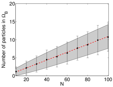
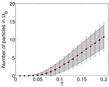
we see that the measured mean values match well with the expected outcomes. For the standard deviations, however, we see that for all values of $T_{\mathrm{final}}^{*}$ and $N$ the measured outcomes are higher than expected. This is an undesired effect and the next section will discuss a way to reduce this artefact.

4 A PBD algorithm with an overlap region

In Section 3.4 we saw that the immediate return of particles from $\Omega_{P}$ into $\Omega_{B}$ in combination with relatively low concentrations close to the interface can lead to errors in the variance of particle concentrations in $\Omega_{B}$. One way to overcome this problem is the introduction of an overlap region where BD simulation and a continuum description exist in parallel, i.e. we will consider the case [B] defined in Section 2 by $\Omega_{B}\cap\Omega_{P}\not=\emptyset$. A sketch of this new set up can be seen in Figure 7 with the overlap region denoted as $O=\Omega_{B}\cap\Omega_{P}$. We also denote the interfaces $I_{1}$ and $I_{2}$ by

$$I_{1}=\partial\Omega_{B}\cap\Omega_{P},\qquad I_{2}=\Omega_{B}\cap\partial\Omega_{P}.$$

In the case of diffusion only, this new setup requires only subtle changes in the algorithm. Molecules are now incorporated into the concentration when they cross the boundary $I_{1}$. The definition of $\widetilde{p}$ is still equal to (14), but we have to redefine $\alpha(t+\Delta t)$ and $p_{2}(x,t+\Delta t)$ as follows

$$\alpha(t+\Delta t) = \int_{\Omega_{B}\setminus\Omega_{P}}\widetilde{p}(x,t+\Delta t)\,\mathrm{d}x\,,$$ (20)

$$p_{2}(x,t+\Delta t) = \frac{\widetilde{p}(x,t+\Delta t)}{\alpha(t+\Delta t)}\,,\qquad\mbox{for}\;x\in\Omega_{B}\setminus\Omega_{P}\,.$$ (21)

The introduction of the overlap region prevents undesired effects generated by molecules crossing over and coming back straight away, as discussed in the thought experiment in Section 3.4. In particular, a molecule initialized as a Dirac $\delta$ function in $\Omega_{P}\setminus\Omega_{B}$ initially contributes very little to the overall probability density near the interface $I_{2}$; by the time it has a significant probability of crossing $I_{2}$ its distribution has become sufficiently spread that it is ‘lost’ in the subdomain $\Omega_{P}$ as is required for the continuous distribution. One time step of the second PBD algorithm is presented in Table 2. As before, we consider that the time step $\Delta t$ is chosen so small that $\alpha(t+\Delta t)\ll 1$. Therefore, we only need to implement cases (i)–(ii) in step (B2), because the probability that two or more molecules are initiated in $\Omega_{B}$ during one time step is negligible.

\begin{overpic}[width=260.17464pt]{./Figure4_1} \put(20.0,2.0){\Large$\Omega_{P}$} \put(70.0,2.0){\Large$\Omega_{B}$} \put(47.0,2.0){\Large$O$} \put(39.0,2.0){\Large$I_{1}$} \put(56.0,2.0){\Large$I_{2}$} \put(20.0,45.0){\color[rgb]{0,0,1}\Large$p(x,t)$} \put(70.0,45.0){\Large$N_{B}(t)$} \put(57.0,34.0){\color[rgb]{0.13,0.55,0.13}\large$x_{i}(t)$} \put(80.0,34.0){\color[rgb]{0.13,0.55,0.13}\large$x_{j}(t)$} \put(94.0,20.0){\large$t$} \put(50.0,-5.0){\Large$x$} \end{overpic}

Fig. 7: Sketch of the PBD algorithm with overlap region and the notation related to it. In $\Omega_{P}$, molecules are described by their density distribution $p(x,t)$, in the microscopic domain $\Omega_{B}$ described by the number $N_{B}(t)$ of molecules and their positions $x_{i}(t)$, $i=1,\dots,N_{B}(t)$. In the overlap region $O$, both descriptions exist in parallel. The interfaces between the various subdomains are denoted $I_{1}$ and $I_{2}$.

1. Calculate $\widetilde{p}(x,t+\Delta t)$ using (14) and $\alpha(t+\Delta t)$ using (20).

2. Generate uniformly distributed random number $r$ in $(0,1)$.

   1. If $r<\alpha(t+\Delta t)$, then create new particle in $\Omega_{B}\setminus\Omega_{P}$ according to the probability density $p_{2}(x,t+\Delta t)$ defined in (21). Set $\beta=\beta_{(i)}$ where $\beta_{(i)}$ is given by (19). Set $N_{B,1}=1.$

   2. If $r\geq\alpha(t+\Delta t)$, then set $\beta=\beta_{(ii)}$ where $\beta_{(ii)}$ is given by (19).
      Set $N_{B,1}=0.$

3. Compute positions $x_{i}(t+\Delta t)$, $i=1,2,\dots,N_{B}(t)$, of BD particles according to (4).

4. Compute new concentration in $\Omega_{P}$ by

   $$p(x,t+\Delta t)=\beta\,\widetilde{p}(x,t+\Delta t)+\sum_{x_{i}(t+\Delta t)\in\Omega_{P}\setminus\Omega_{B}}\!\!\!\!\!\delta(x-x_{i}(t+\Delta t))\,,\quad\mbox{for}\;x\in\Omega_{P}\,.$$

5. Update the number of BD particles by

   $$N_{B}(t+\Delta t)=N_{B}(t)+N_{B,1}-\left|\left\{x_{i}(t+\Delta t)\in\Omega_{P}\setminus\Omega_{B}\;,i=1,\dots,N_{B}(t)\right\}\right|\,.$$

   Terminate computation of trajectories of BD molecules which landed in $\Omega_{P}\setminus\Omega_{B}$ (i.e. the BD particles which satisfy $x_{i}(t+\Delta t)\in\Omega_{P}\setminus\Omega_{B}.$)
   Then continue with step (B1) for time $t+\Delta t$.

Table 2: One time step of the PBD algorithm with overlap region for system of diffusing molecules.

In order to highlight the advantages of the overlap region, we simulate the same diffusion process as in Figure 4 with $\Omega_{P}=(-1,0)$ and $\Omega_{B}=(-0.1,1)$. Then the overlap region is $O=\Omega_{P}\cap\Omega_{B}=(-0.1,0)$. The results are shown in Figure 8. As before, the mean outcome matches well with the exact solution, with stochastic fluctuations inside the overlap region $O$ due to the mixed description. In Figure 8(b) we see that the introduction of the overlap region indeed reduced the problem of high variances inside $\Omega_{B}\setminus\Omega_{P}$.

(a) Mean

(b) Variance

Fig. 8: Simulation results of a diffusion process in $\Omega=(-1,1)$ with no flux boundary conditions and initial conditions $n(x,0)=100\delta(x+0.95)$ with $\Omega_{P}=(-1,0)$, $\Omega_{B}=(-0.1,1)$ and $O=(-0.1,0)$ averaged over 1000 realisations. Dashed (red) line: expected outcome. (a) Solid line: mean value in $\Omega_{P}$; bars: particle concentrations in $\Omega_{B}\setminus O$ (gray) and $O$ (green). (b) (Gray) bars: measured variances in particle concentrations. Parameter values as for Figure 4.

A proof similar to Theorem 1 can be used to show that the PBD algorithm (B1)–(B5) satisfies Conditions (C.1) and (C.3) for $\Delta t>0$. We will now further show that the algorithm describes a diffusion process exactly in the limit $\Delta t\to 0$.

Theorem 2.

Suppose that a PDE-description of the system is used in $\Omega_{P}=(-\infty,0)$, and a BD simulation in $\Omega_{B}=(-d,\infty)$ with the overlap region $O=(-d,0)$ where $d>0$. In the limit that $\Delta t\rightarrow 0$ the expected concentration distribution $P_{P}(x,t)={\mathbb{E}}[p(x,t)]$ in the continuum regime and the expected concentration distribution $P_{B}(x,t)$ in the BD regime obey the equations

$$\frac{\partial P_{P}}{\partial t} =D\frac{\partial^{2}P_{P}}{\partial x^{2}}+\left.D\frac{\partial P_{B}}{\partial x}\right|_{x\rightarrow-d_{+}}\delta\left(x+d\right),\quad\ x\in\Omega_{P}\,,$$ (22)

$$\frac{\partial P_{B}}{\partial t} =D\frac{\partial^{2}P_{B}}{\partial x^{2}}-\left.D\frac{\partial P_{P}}{\partial x}\right|_{x\rightarrow 0_{-}}\delta\left(x\right),\quad\ x\in\Omega_{B}\,,$$ (23)

where

$$P_{P}(0,t)=0\,,\qquad P_{B}(-d,t)=0\,,\qquad\mbox{for}\quad t>0.$$

Extend each distribution to the whole line by defining $P_{P}(x,t)=0$ for $x\in(0,\infty)$ and $P_{B}(x,t)=0$ for $x\in(-\infty,-d)$. Then the sum of these two processes $n(x,t)=P_{P}(x,t)+P_{B}(x,t)$, $x\in\Omega$, $t>0$ satisfies the diffusion equation (9).

Proof.

Consider the function

$$n(x,t)=P_{P}(x,t)+P_{B}(x,t).$$ (24)

Clearly

$$\frac{\partial n}{\partial t}=D\frac{\partial^{2}n}{\partial x^{2}}\qquad\mbox{ for }x\in(-\infty,-d)\cup(-d,0)\cup(0,\infty).$$

Since each of $P_{P}$ and $P_{B}$ is continuous at $x=-d$ and $x=0$, function $n$ will be continuous there. Moreover, since

$$\left[\frac{\partial P_{P}}{\partial x}\right]^{x=0_{+}}_{x=0_{-}}=-\frac{\partial P_{P}}{\partial x}\left(0_{-},t\right),\qquad\left[\frac{\partial P_{B}}{\partial x}\right]^{x=0_{+}}_{x=0_{-}}=\frac{\partial P_{P}}{\partial x}\left(0_{-},t\right),$$

$\partial n/\partial x$ is continuous at $x=0$. Similarly, since

$$\left[\frac{\partial P_{P}}{\partial x}\right]^{x=-d_{+}}_{x=-d_{-}}=-\frac{\partial P_{B}}{\partial x}\left(-d_{+},t\right),\qquad\left[\frac{\partial P_{B}}{\partial x}\right]^{x=-d_{+}}_{x=-d_{-}}=\frac{\partial P_{B}}{\partial x}\left(-d_{+},t\right),$$

$\partial n/\partial x$ is also continuous at $x=-d$. By standard regularity results this is enough to guarantee that $n$ satisfies the diffusion equation on the whole real line. ∎

Remark. For the overlap region to give a different result from the simple PDB algorithm (A1)–(A5), we should choose $d$ much bigger than the mean displacement $\sqrt{2D\Delta t}$ of a particle given the time step $\Delta t$ as defined in (4).

4.1 Dependence of the variance on the system parameters

In order to show that the variances are indeed accurately produced by the PBD algorithm (B1)–(B5), we repeated the numerical experiments conducted in Section 3.4.1. We chose $\Omega_{P}=(-1,0)$, $O=(-0.1,0)$ and $\Omega_{B}=(-0.1,1)$ and measure the number molecules situated in $\Omega_{B}\setminus\Omega_{P}=[0,1)$ at the end of the simulation. We again calculate the mean values and standard deviation and present the results in Figure 9.

(a) $N=10,20,\dots,100,\quad T_{\mathrm{final}}^{*}=0.2$

(b) $T_{\mathrm{final}}^{*}=0.01,0.02,\dots,0.2,\quad N=100$

Fig. 9: Mean values and standard deviations of the number of particles in $\Omega_{B}\setminus\Omega_{P}$ at time $T_{\mathrm{final}}^{*}$ depending on $T_{\mathrm{final}}^{*}$ and $N$. Dashed line: expected number of particles; shaded area: expected standard deviation; dots: measured mean values; error bars: measured standard deviations. Parameters as for Figure 8.

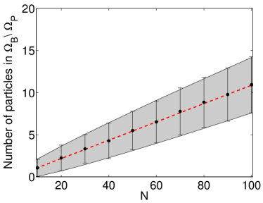
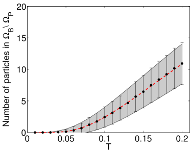
We can clearly see that the adjusted algorithm produces more accurate standard deviations than the original algorithm, whilst keeping the mean values correct. We conclude that the algorithm (B1)–(B5) produces an accurate BD simulation inside $\Omega_{B}\setminus\Omega_{P}$ and therefore satisfies the Conditions (C.1)–(C.3). We will use the PBD algorithm (B1)–(B5) in the remainder of this paper.

5 Reaction-diffusion systems

In the next step we introduce chemical reactions into the system presented in Section 4. We will concentrate on zero-order and first-order reactions [12]. First-order reactions are reactions which only have one reactant, for example,

$$X_{1}\ \stackrel{{\scriptstyle k_{1}}}{{\longrightarrow}}\ X_{2}\,,\qquad\mbox{or}\qquad X_{1}\ \stackrel{{\scriptstyle k_{2}}}{{\longrightarrow}}\ X_{4}+X_{5}\,,$$ (25)

where $X_{i}$ denote chemical species and $k_{1}$ (resp. $k_{2}$) the corresponding rate constant (which has physical units $[$sec${}^{-1}]$). In what follows, we will denote by $\emptyset$ chemical species which are of no interest to a modeller. Then, considering that $X_{1}$ is the only chemical species of interest, we can rewrite the reactions (25) as

$$X_{1}\ \stackrel{{\scriptstyle k_{d}}}{{\longrightarrow}}\ \emptyset,$$ (26)

where $k_{d}=k_{1}+k_{2}$. We will also consider zero-order reactions. An example is:

$$\emptyset\ \stackrel{{\scriptstyle k_{p}}}{{\longrightarrow}}\ X_{1},$$ (27)

where the rate constant $k_{p}$ has physical units $[$M sec${}^{-1}]$, i.e. it is the production rate per unit of volume and unit of time. It is relatively straightforward to implement zero-order and first-order chemical reactions in the PBD algorithms (A1)–(A5) and (B1)–(B5), because these reactions can be treated in the individual parts of the system (continuum and BD simulation) independently. Note that for higher-order reactions this is not necessarily the case, as particles could react with the continuum inside the overlap region $O$. This case is not discussed in this paper.

In the continuum regime reactions are represented by the term $R_{j}(p_{1},p_{2},\dots,p_{M})$ on the right-hand side of the reaction-diffusion PDE (1). For example, if the chemical species $X_{1}$ is subject to chemical reactions (26)–(27), then the reaction-diffusion PDE (1) takes the form

$$\frac{\partial p_{1}}{\partial t}=D_{1}\frac{\partial^{2}p_{1}}{\partial x^{2}}-k_{d}\,p_{1}+k_{p}\,.$$

In the BD simulations, the molecules act independently and the reactions can therefore be treated individually. A summary of how to implement various reactions in BD simulations can be found in [12].

Although implementation of the zero-order and first-order reactions is relatively straighforward, one has to still consider some special effects that are related to the coupling of the two parts of the domain. First, what happens when a particle that is supposed to react at time $t_{1}$ crosses the interface $I_{1}$ at an earlier time $t_{2}<t_{1}$? Since we assumed that all information about particles is lost as soon as they cross the interface $I_{1}$, we incorporate it into the continuum and the reaction at time $t_{1}$ does not happen. Second, what happens when a particle is created inside the overlap region $O$? A number of solutions to this problem are possible: one could split the creation in equal parts, or declare creation to only contribute to either the continuum or the molecular-based description. We will here assume that all creation inside the overlap region occurs in the form of molecules with exact positions.

Finally, let us note that (reactive) boundary conditions on the external boundary $\partial\Omega$ can be treated according to the corresponding modelling regime, i.e. whether the corresponding segment of $\partial\Omega$ is part of $\partial\Omega_{P}$ or $\partial\Omega_{B}$. Derivation of reactive boundary conditions of BD simulations which are consistent with the PDE description can be found in [8]. External boundaries slightly modify the computation of $\widetilde{p}(x,t+\Delta t)$ in $\Omega_{P}$. It is still given by (14) but the kernel (15) has to be updated to take into account the boundary condition imposed on the external boundary $\partial\Omega$. We have already done this when we showed simulations of the diffusion process in Figures 4 and 8 in the finite interval $(-1,1)$ with no flux boundary conditions. However, for small timesteps $\Delta t$ the change is negligible, since all the action takes place near the interface $I_{2}$.

We conclude this section with three examples which illustrate the behaviour of the PBD algorithm (B1)–(B5) for reaction-diffusion systems. They include the modelling of morphogen gradients and chemisorption.

5.1 Example 1: morphogen gradient

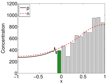
In the first example we compute a steady state for a morphogen gradient model [28, 32, 20]. We consider one chemical species (morphogen) inside the domain $\Omega=(-1,1)$. All parameters are dimensionless for simplicity. The only reaction inside $\Omega=(-1,1)$ is the degradation (26). Additionally to this reaction, we assume a constant influx $J/D$ through the left-hand boundary $x=-1$ to the continuum subdomain $\Omega_{P}=(-1,0)$. We use $O=(-0.1,0)$ and $\Omega_{B}=(-0.1,1)$ with a no flux boundary at $x=1$. Since we only have first-order reaction (26), the exact solution $n(x,t)$ is given by

$$\frac{\partial n}{\partial t}=D\frac{\partial^{2}n}{\partial x^{2}}-k_{1}n\,,\qquad\frac{\partial n}{\partial x}(-1,t)=-J\,,\qquad\frac{\partial n}{\partial x}(1,t)=0\,.$$ (28)

This system is initialised with $n(x,0)=0$, $x\in\Omega$, and we let it run until it (approximately) reaches the steady state. We use $J=1000$ and $k_{1}=1$. The second PBD algorithm (B1)–(B5) is run with the same parameters presented in Section 4 for time $T_{\mathrm{final}}=20$ which is (approximately) a time at which the model settles into the steady state. The reaction (26) is simulated in a time-driven manner in $\Omega_{B}$, which means that for each morphogen molecule it is decided randomly at the end of each time step whether it was degraded or not (the probability of degradation of each molecule is equal to $k_{d}\,\Delta t$ provided that $k_{d}\,\Delta t\ll 1$).

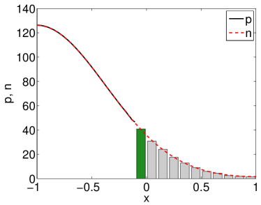
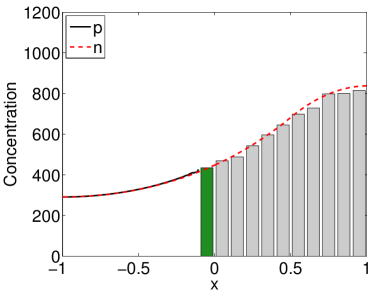
The result of a single simulation of the PBD algorithm (B1)–(B5) is plotted in Figure 10(a). We plot the PDE solution in $\Omega_{P}\setminus O$ as a black line and the (gray) histogram of molecules in $\Omega_{B}\setminus O$. In the overlap region $O$, we compute the total “number” of particles by

$$N_{O}(T_{\mathrm{final}})\equiv\int_{O}p(x,T_{\mathrm{final}})\mathrm{d}x+\big{|}\left\{x_{i}(T_{\mathrm{final}})\in O\;,i=1,2,\ldots,N_{B}(T_{\mathrm{final}})\right\}\big{|}.$$ (29)

The value of $N_{O}(T_{\mathrm{final}})$ is plotted as the green bar in Figure 10(a). The results of a single simulation of the PBD algorithm (B1)–(B5) are compared with the exact solution, which is obtained by solving the PDE (28) numerically until time $T_{\mathrm{final}}$. In this simple example, it is also possible to find an analytical expression for the steady state profile which is approximately equal to the presented dashed line.

Note that the jagged appearance of the continuum solution close to the interface is not numerical error, but represents the fact that as molecules cross from the discrete to the continuum side information about their exact location is lost gradually over time (remember that Figure 10(a) shows just one realisation of the stochastic process). The corresponding distribution on the discrete side $\Omega_{B}\setminus\Omega_{P}$ would be $\delta$ function spikes at the location of the particles, which we have in effect locally averaged by our binning process. Thus the jaggedness can be seen as a gradual transition in the solution from isolated discrete particles to a continuum density distribution. An ensemble average over 100 simulations of the PBD algorithm (B1)–(B5) is shown in Figure 10(b). The stochastic fluctuations are reduced compared to the single simulation and the results compare well with the exact solution for the expected probability density (28).

(a) Single simulation

(b) Average over 100 realisations

Fig. 10: Simulation results for Example 1. Dashed (red) line: exact solution given by $(\ref{eq:exp1:full})$; solid line: $p(x,T_{\mathrm{final}})$; (gray) bars: spatial concentration of particles at $t=T_{\mathrm{final}}$ in $\Omega_{B}\setminus O$; (green) bar: $N_{O}(T_{\mathrm{final}})$ given by $(\ref{numberoverlap})$. Parameters as described in the text.

5.2 Example 2: reversed morphogen gradient

In this example we introduce a second reaction in addition to (26) – a local production of molecules:

$$\emptyset\ \stackrel{{\scriptstyle k_{p}}}{{\longrightarrow}}\ A\qquad\mbox{in }[x_{s},1]\,,$$ (30)

where $x_{s}$ defines the size of the creation zone. As before we consider all parameters to be dimensionless: $k_{p}$ is defined as the rate of production per unit length. For this system we use no flux boundary conditions on both ends. The combination of localized production (30) and degradation (26) ensures that the system settles into a non-trivial steady-state which we will compute with the PBD algorithm (B1)–(B5). The exact solution (which the PBD algorithm (B1)–(B5) approximates) can be described by

$$\frac{\partial n}{\partial t}=D\frac{\partial^{2}n}{\partial x^{2}}-k_{1}n+k_{2}\chi_{[x_{s},1]}\,,\qquad\frac{\partial n}{\partial x}(-1,t)=0\,,\qquad\frac{\partial n}{\partial x}(1,t)=0\,,$$ (31)

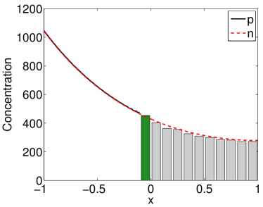
where $\chi_{[x_{s},1]}$ is the characteristic function for the interval $[x_{s},1]$ that takes the value $1$ inside and $0$ outside of the interval. The production reaction (30) was implemented in BD simulations in an event-driven way, such that particles can get created at any time in-between time steps and the number of particles created in one time step is not limited. We used $k_{p}=1$, $k_{d}=2000$ and $x_{s}=0.5$. For the PBD simulations we use the same parameters as in Section 4. In particular, we have $\Omega_{P}=(-1,0)$, $O=(-0.1,0)$ and $\Omega_{B}=(-0.1,1)$.

A single realisation of this process is plotted in Figure 11(a). We plot the PDE solution in $\Omega_{P}\setminus O$ as a black line. The concentration of molecules in $\Omega_{B}\setminus O$ is visualized as a (gray) histogram. In the overlap region $O$, we plot $N_{O}(T_{\mathrm{final}})$ given by (29). The concentration gradient is now reversed, as the creation of particles happens near the right-hand boundary. Again, one can clearly see the stochastic fluctuations in this plot which also have effects on the value of $p(x,t)$ far from the overlap region $O$. However, as we draw an ensemble average over 100 simulations in Figure 11(b), the results converge towards the exact solution which is obtained by solving the PDE (31). It is plotted as a (red) dashed line in Figure 11.

(a) Single simulation

(b) Average over 100 simulations

Fig. 11: Simulation results for Example 2. Dashed (red) line: exact solution given by $(\ref{eq:exp2:full})$; solid line: $p(x,T_{\mathrm{final}})$ in $\Omega_{P}\setminus O$; (gray) bars: spatial concentration of particles at $t=T_{\mathrm{final}}$ in $\Omega_{B}\setminus O$; (green) bar: $N_{O}(T_{\mathrm{final}})$ given by $(\ref{numberoverlap})$. Parameters as described in the text.

5.3 Example 3: chemisorption

Our last example is the polymer coating of a virus surface [14, 11]. We will describe it as irreversible adsorption (chemisorption) of polymers to a two-dimensional surface as was introduced in [9]. This example presents a typical application area of PBD algorithms. A detailed model is used close to the reactive boundary where positions of individual molecules influence the dynamics of diffusion-driven adsorption. On the other hand, a less detailed model can be used far away from the adsorbing surface. In the bulk the behaviour of reactive polymers can be described by the macroscopic reaction-diffusion PDE (1) in the form

$$\frac{\partial p}{\partial t}=D\frac{\partial^{2}p}{\partial z^{2}}-k_{d}\,p\,.$$ (32)

in the semi-infinite domain $\Omega=(0,\infty)$ (here, $z$ is the distance from the reactive surface which is at $z=0$). This equation takes into account two processes which mainly influence chemisorption dynamics [9]: diffusion of polymer molecules and the hydrolysis of reactive groups in the solution. Both processes can be implemented in the BD context as we saw in the previous examples. However, this level of detail is only needed close to the virus surface.

Whenever a polymer molecule interacts with the surface, it is either reflected or (irreversibly) adsorbed. The chemisorption is modelled by a random sequential adsorption (RSA) algorithm [7]: we check whether the corresponding binding site on the surface is free and then the reaction occurs with a certain probability. This probability is related to the reaction rate constant of the binding reaction as given in [8]. The reader can find more details about the model in [9]. In this paper, we show that the PBD algorithms can be used to compute the results from [9]. We will use the same parameters, namely $D=5\times 10^{-5}\,\mbox{mm}^{2}\,\mbox{s}^{-1}$, $k_{d}=1.3\times 10^{-4}\,\mbox{s}^{-1}$ and $\Delta t=0.01\,\mbox{s}$. Then the mean displacement per time step according to (4) is $\sqrt{2D\Delta t}=10^{-3}\,\mbox{mm}$ and we therefore choose the size of the overlap region of the PBD algorithm (B1)–(B5) as $|O|=10^{-2}\,\mbox{mm}$. From the results in [9], we estimate that a maximum length of $L=2\,\mbox{mm}$ is enough to simulate the binding process and use the Dirichlet boundary condition

$$n(L,t)=c_{0}\exp(-k_{d}t)\,,$$

where $c_{0}=1.2\times 10^{4}\,\mbox{molecules}/\mbox{mm}$ is the initial concentration of molecules (i.e. $n(z,0)\equiv c_{0}$ for $z\in\Omega$). To apply the PBD algorithm (B1)–(B5), we choose $\Omega_{B}=[0,1.01)\,\mbox{mm}$, $O=(1,1.01)\,\mbox{mm}$ and $\Omega_{P}=(1,2)\,\mbox{mm}$. The RSA algorithm was performed using a nearest neighbour exclusion on a $100\times 100$ grid of receptor binding positions on the surface [7].

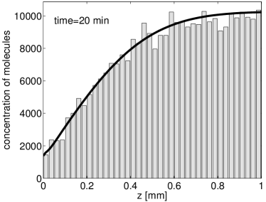
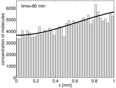
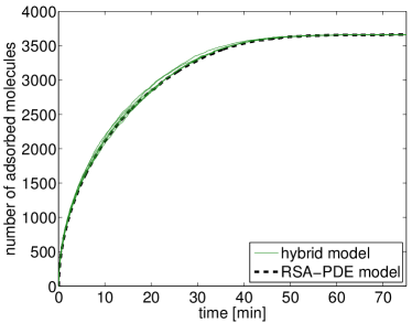
In Figure 12 we plot the concentration profile inside $\Omega_{B}$ of a single simulation at two different times (gray histograms). We compare the results of the PBD algorithm (B1)–(B5) with the results of the RSA-PDE model presented in [9] (black lines). As shown in [9], the RSA-PDE model also compares well with the full BD simulation. The number of molecules which are attached to the surface as a function of time is plotted in Figure 13 (six realisations of the PBD algorithm (B1)–(B5) are plotted as green solid lines). Again, we see an excellent agreement with the result from [9] which is plotted as the black dashed line.

(a) $T_{\mathrm{final}}=20min$

(b) $T_{\mathrm{final}}=80min$

Fig. 12: Example 3 (chemisorption to virus surface). (Gray) histograms: concentration profile in molecules/mm at two given times computed by the PBD algorithm (B1)–(B5); solid line: results of the RSA-PDE model presented in [9]. Parameters as shown in the text.

Fig. 13: Example 3 (chemisorption to virus surface). Number of polymer molecules which are bound to the virus surface as a function of time. (Green) solid lines: six realisations computed by the PBD algorithm (B1)–(B5); (black) dashed line: results of the RSA-PDE model presented in [9]. Parameters as shown in the text.

6 Discussion

In this paper we have presented two PBD algorithms that combine Brownian dynamics with mean-field reaction-diffusion PDEs. This method produces exact Brownian dynamics simulations in one part of the domain and couples them with mean field approximations in another part of the domain. An algorithm of this type is useful for various application areas in computational biology and beyond, for example, when a detailed description of individual molecules is required near a receptor or ion channel, but becomes impractical in the bulk of a cell [5, 16]; or when a detailed stochastic simulation of actin dynamics is required inside filopodia, but becomes impractical in the bulk of a cell [33]. Another application area, chemisorption, was discussed in Section 5.3. By using our approach it would also be possible to use finite-sized particles in the BD simulation and couple these with the corresponding mean field results presented in [3].

In the literature several hybrid models have been developed in the context of fluid dynamics, but they do not discuss issues that arise from the incorporation of chemical reactions. Alexander et al [1] presents a hybrid model that uses virtual particles at the grid point nearest to the interface to calculate fluxes across the boundary and to generate accurate density fluctuations inside the particle region. Reference [31] extends this approach by the introduction of an overlap region similar to $O$ introduced in Section 4. An identical flux exchange with particles confined to a grid is presented in [17]. Chemical reactions in the solution were considered in [9]. This model was discussed in Section 5.3. It couples Brownian dynamics of molecules in the solution with a more detailed description of the adsorbing boundary. In [9] a hybrid (RSA-PDE) model has been developed which replaces BD in the solution by solving the PDE (32) with a suitable stochastic boundary condition. The PBD algorithms are able to replace the stochastic boundary condition by a (small) BD region close to the surface. Although the hybrid RSA-PDE model introduced in [9] was sufficient in the case of (irreversible) adsorption, the situation is becoming more challenging whenever the binding reaction is reversible [21]. In this case, a molecule which is released by the surface will initially stay close to the surface and can rebind to the same receptor (binding site). This geminate recombination can be captured by the PBD approach. Reversible reactions are common in biological applications [21, 16].

Hybrid approaches for reaction-diffusion processes which couple different modelling approaches have also been introduced in the literature [23, 15, 6, 13]. A mesoscopic lattice-based description coupled with macroscopic Fisher-Kolmogorov-Petrovsky-Piscounov PDE was used in [23] to study front propagation in a lattice-based reaction-diffusion model. A hybrid model for reaction-diffusion systems in porous media that combines pore-scale models with Darcy-scale models is presented in [27]. Flegg et al [15] introduced the so-called Two Regime Method which couples a lattice-based (compartment-based) reaction-diffusion model with BD simulations. One advantage of the PBD algorithms over the Two Regime Method is that there are more efficient tools for PDE simulations than for compartment-based reaction-diffusion models. On the other hand, compartment-based models provide more details (including fluctuations) and hybrid models which couple BD simulations with compartment-based models do not require the overlap region [15, 13]. Since it is possible to couple the macroscopic PDE description with (mesoscopic) compartment-based models [6] and compartment-based models with (microscopic) BD simulations [15], then an alternative approach to PBD algorithms would be to use compartment-based models in the overlap region. That is, the computational domain would be divided into three regions where the PDE, compartment-based and BD descriptions would be used. These three regimes would be coupled using the results from the literature [6, 15]. Compartment-based models and macroscopic PDEs can also be coupled through another intermediate regime using a tau-leap method [13]. In this paper, we showed that PDE models and BD simulations can be coupled without using intermediate compartment-based models.

The PBD algorithms presented in this paper should be seen as a first step towards a more general setting. Some parts of the algorithm (B1)–(B5) extend easily (at least theoretically) into higher dimensions, but in practice additionally difficulties are posed. One example is the necessity to sample from a multidimensional probability distribution to find the position of newly created molecules. Additionally, in higher dimensions one can also expect to deal with higher order reactions, including bimolecular reactions. For a discussion of how to implement bimolecular reactions for BD simulations, we refer to [10], but the real problem occurs inside the overlap region $O=\Omega_{B}\cap\Omega_{P}$, where a molecule could react with another molecule, or with the continuum. Since the reaction-diffusion PDEs are solved numerically using a suitable mesh, it is important to study methods for coupling individual molecules with the numerical discretization of macroscopic PDEs [18]. For the ion channel application mentioned before, one also needs to think about how to incorporate electrical charges and resulting forces into the system. One can imagine that these forces act as a boundary condition on the continuum model and as an effective force on the particles.

References

- [1] F. Alexander, A. Garcia, and D. Tartakovsky, Algorithm refinement for stochastic partial differential equations, Journal of Computational Physics, 182 (2002), pp. 47–66.
- [2] S. Andrews and D. Bray, Stochastic simulation of chemical reactions with spatial resolution and single molecular detail, Physical Biology, 1 (2004), pp. 137–151.
- [3] M. Bruna and S. J. Chapman, Excluded-volume effects in the diffusion of hard spheres, Physical Review E, 85 (2012), p. 011103.
- [4] W. Chen, R. Erban, and S. J. Chapman, From Brownian dynamics to Markov chain: an ion channel example. submitted, 2012.
- [5] B. Corry, S. Kuyucak, and S. Chung, Tests of continuum theories as models of ion channels. i. Poisson-Nernst-Planck theory versus Brownian dynamics, Biophysical Journal, 78 (2000), pp. 2364–2381.
- [6] S. Engblom, L. Ferm, A. Hellander, and P. Lötstedt, Simulation of stochastic reaction-diffusion processes on unstructured meshes, SIAM Journal on Scientific Computing, 31 (2009), pp. 1774–1797.
- [7] R. Erban and S. J. Chapman, On chemisorption of polymers to solid surfaces, Journal of Statistical Physics, 127 (2007), pp. 1255–1277.
- [8] , Reactive boundary conditions for stochastic simulations of reaction-diffusion processes, Physical Biology, 4 (2007), pp. 16–28.
- [9] , Time scale of random sequential adsorption, Physical Review E, 75 (2007), p. 041116.
- [10] , Stochastic modelling of reaction-diffusion processes: algorithms for bimolecular reactions, Physical Biology, 6 (2009), p. 046001.
- [11] R. Erban, S. J. Chapman, K. Fisher, I. Kevrekidis, and L. Seymour, Dynamics of polydisperse irreversible adsorption: a pharmacological example, Mathematical Models and Methods in Applied Sciences (M3AS), 17 (2007), pp. 759–781.
- [12] R. Erban, S. J. Chapman, and P. Maini, A practical guide to stochastic simulations of reaction-diffusion processes. 35 pages, available at http://arxiv.org/abs/0704.1908, 2007.
- [13] L. Ferm, A. Hellander, and P. Lötstedt, An adaptive algorithm for simulation of stochastic reaction-diffusion processes, Journal of Computational Physics, 229 (2010), pp. 343–360.
- [14] K. Fisher, Y. Stallwood, N. Green, K. Ulbrich, V. Mautner, and S. L., Polymer-coated adenovirus permits efficient retargeting and evades neutralising antibodies, Gene therapy, 8 (2001), pp. 341–348.
- [15] M. B. Flegg, S. J. Chapman, and R. Erban, The Two Regime Method for optimizing stochastic reaction-diffusion simulations, Royal Society Interface, 9 (2012), pp. 859–868.
- [16] M. B. Flegg, S. Ruediger, and R. Erban, Diffusive spatio-temporal noise increases IP3R calcium channel puff frequency. submitted, 2012.
- [17] E. Flekkøy, J. Feder, and G. Wagner, Coupling particles and fields in a diffusive hybrid model, Physical Review E, 64 (2001), p. 066302.
- [18] B. Franz and R. Erban, Hybrid modelling of individual movement and collective behaviour, to appear in Dispersal, individual movement and spatial ecology: A mathematical perspective, M. Lewis, P. Maini, and S. Petrovskii, eds., Springer, 2012.
- [19] J. Hattne, D. Fange, and J. Elf, Stochastic reaction-diffusion simulation with MesoRD, Bioinformatics, 21 (2005), pp. 2923–2924.
- [20] M. Howard, How to build a robust intracellular concentration gradient, Trends in Cell Biology, 22 (2012), pp. 311–317.
- [21] J. Lipkova, K. Zygalakis, S. J. Chapman, and R. Erban, Analysis of brownian dynamics simulations of reversible bimolecular reactions, SIAM Journal on Applied Mathematics, 71 (2011), pp. 714–730.
- [22] K. Lipkow, S. Andrews, and D. Bray, Simulated diffusion of phosphorylated chey throughthe cytoplasm of escherichia coli, Journal of Bacteriology, 187 (2005), pp. 45–53.
- [23] E. Moro, Hybrid method for simulating front propagation in reaction-diffusion systems, Physical Review E, 69 (2004), p. 060101.
- [24] G. Moy, B. Corry, S. Kuyucak, and S. Chung, Tests of continuum theories as models of ion channels. i. Poisson-Boltzmann theory versus Brownian dynamics, Biophysical Journal, 78 (2000), pp. 2349–2363.
- [25] J. Murray, Mathematical Biology II: Spatial Models and Biomedical Applications, Springer, 3rd ed., 2003.
- [26] K. Takahashi, S. Tanase-Nicola, and P. ten Wolde, Spatio-temporal correlations can drastically change the response of a mapk pathway, PNAS, 107 (2010), pp. 19820–19825.
- [27] A. Tartakovsky, D. Tartakovsky, T. Scheibe, and P. Meakin, Hybrid simulations of reaction-diffusion systems in porous media, SIAM Journal of Scientific Computing, 30 (2008), pp. 2799–2816.
- [28] F. Tostevin, P. ten Wolde, and M. Howard, Fundamental limits to position determination by concentration gradients, PLOS Computational Biology, 3 (2007), pp. 763–771.
- [29] J. van Zon and ten Wolde P., Simulating biochemical networks at the particle level and in time and space: Green’s function reaction dynamics, Physical Review Letters, 94 (2005), p. 128103.
- [30] J. von Neumann, Mathematical Foundations of Quantum Mechanics, Princeton University Press, 1955.
- [31] G. Wagner and E. Flekkøy, Hybrid computations with flux exchange, Philosophical Transactions of the Royal Society A: Mathematical, Physical & Engineering Sciences, 362 (2004), pp. 1655–1665.
- [32] L. Wolpert, R. Beddington, T. Jessel, P. Lawrence, E. Meyerowitz, and J. Smith, Principles of Development, Oxford University Press, 2002.
- [33] P. Zhuravlev and G. Papoian, Molecular noise of capping protein binding induces macroscopic instability in filopodial dynamics, Proceedings of the National Academy of Sciences (PNAS), 106 (2009), pp. 11570–11575.