Kronecker covers, V-construction,

unit-distance graphs and isometric

point-circle configurations

Gábor Gévay

Bolyai Institute, University of Szeged

Aradi vértanúk tere 1, H-6720 Szeged

Hungary

gevay@math.u-szeged.hu

and

Tomaž Pisanski

Faculty of Mathematics and Physics

University of Ljubljana, Jadranska 19, 1111 Ljubljana

Slovenia

Tomaz.Pisanski@fmf.uni-lj.si

Abstract

We call a polytope $P$ of dimension 3 admissible if it has the following two properties: (1) for each vertex of $P$ the set of its first-neighbours is coplanar; (2) all planes determined by the first-neighbours are distinct. It is shown that the Levi graph of a point-plane configuration obtained by $V\!$-construction from an admissible polytope $P$ is the Kronecker cover of its 1-skeleton. We investigate the combinatorial nature of the $V$-construction and use it on unit-distance graphs to construct novel isometric point-circle configurations. In particular, we present an infinite series whose all members are subconfigurations of the renowned Clifford configurations.

Keywords: V-construction, unit-distance graph, isometric point-circle configuration, Kronecker cover, Clifford configuration, Danzer configuration, generalized cuboctahedron graph.

Math. Subj. Class.: 05B30, 51A20, 52B10, 52C30

1 Introduction.

In this paper we investigate and carry over from polytopes to graphs the so-called $V\!$-construction, which was originally introduced in [16]. In this process we explain the construction in terms of the canonical double cover, also called the Kronecker cover of graphs. The reader is referred to [28] for graph coverings and to the monographs [21, 34] for the background on configurations and their Levi graphs.

The first author used convex 3-polytopes in order to define a construction of geometric point-plane configurations in the following way [16].

Let $P$ be a polytope of dimension 3 with the property that for each vertex $v$ the set of its first neighbours $P(v)$ is coplanar. In particular, this will always be true if the graph (or 1-skeleton) of the polytope $P$ is trivalent. There are several other classes of polytopes that have this property. Furthermore, we assume that all planes obtained in this way are distinct. In particular, this condition rules out bipyramids such as the octahedron. Let us call such a polytope admissible.

Proposition 1.

Each 3-polytope with trivalent 1-skeleton is admissible.

Proof. Since each vertex of a 3-polytope with trivalent 1-skeleton has exactly three first-neighbours, they are clearly coplanar. An easy argument shows that if two trivalent vertices of a 3-polytope $P$ share the same set of first-neighbours, then the 1-skeleton of $P$ itself cannot be trivalent. $\square$

Let $S(P)$ denote the set of such planes as above, if they exist. If $V(P)$ denotes the set of vertices of $P$, then the pair $((V(P),S(P))$ defines a geometric incidence structure of points and planes with the usual incidence. We call this procedure the geometric $V\!$-construction. If the 1-skeleton of $P$ is a regular, say $k$-valent graph, then each point of the configuration will sit on $k$ planes. It immediately follows from the definition that each plane contains exactly $k$ points. Let $n$ be the number of vertices of $P$. Therefore, combinatorially, the incidence structure is an $(n_{k})$ configuration.

A natural question is that what is the Levi graph of such a configuration. Recall that the Levi graph $L(C)$ of a configuration $C$ is a bipartite graph whose bipartition classes consist of the points and “blocks” of $C$, respectively, and two points in $L(C)$ are adjacent if and only if the corresponding point and “block” in $C$ are incident. Levi graphs are useful tools in studying configurations, because of the following property [9].

Lemma 2.

A configuration $C$ is uniquely determined by its Levi graph $L(C)$.

Another, much more difficult question is, if we can find any conditions under which such a combinatorial configuration may be realized geometrically as configuration of points and lines. On the other hand, it may happen that a configuration can be realized in both a point-line and a point-plane version (cf. our Example in Section 2). In Section 3 and 5 we also present examples for configurations of which both point-line and point-circle realization exist.

Point-circle configurations themselves are also interesting, since, in contrast to the point-line configurations, relatively little is known about them. The most notable achievement in this respect is undoubtedly Clifford’s infinite series of configurations, going back to 1871 [10, 21]. In the last two sections we present a new construction of Clifford’s configurations, as well as three new infinite series of point-circle configurations.

We note that the construction introduced in [16] is more general than needed here: instead of 3-dimensional polytopes one can take $d$-dimensional polytopes and accordingly, instead of planes one should consider hyperplanes. Also, instead of first-neighbours it is possible to consider second-neighbours. However, we do not consider these aspects of the $V\!$-construction here.

2 Combinatorial $V\!$-construction.

Let us generalize and carry out the $V\!$-construction on the abstract level.

To any regular graph $G$ we may associate a combinatorial configuration. For a vertex $v$ of $G$, denote by $N(v)$ the set of vertices adjacent to $v$. Then take the family $S(G)$ of these vertex-neighbourhoods:

$$S(G)=\{N(v)\,|\,v\in V(G)\}.$$

The triple $(V(G),S(G),\in)$ defines a combinatorial incidence structure, underlying the geometric configuration of points and planes for any 3-polytope $P$ whose 1-skeleton is $G$. We shall denote this structure by $N(G)$.

We note that a closely related construction occurs in the context of combinatorial geometries [30, 37].

The following general result establishes a connection between Levi graphs and Kronecker covers. It will play a central role in our constructions presented in the rest of the paper. First, we recall that a graph $\widetilde{G}$ is said to be the Kronecker cover (or canonical double cover) of the graph $G$ if there exists a $2:1$ surjective homomorphism $f:\widetilde{G}\rightarrow G$ such that for every vertex $v$ of $\widetilde{G}$ the set of edges incident with $v$ is mapped bijectively onto the set of edges incident with $f(v)$ [28].

Theorem 3.

Let $G$ be a graph on $n$ vertices and let $L$ be the Levi graph of the incidence structure $N(G)$. If no two vertices of $G$ have the same neighbourhood, then $L$ is the Kronecker cover of $G$.

Proof. Under the assumption that no two vertices have the same set of neighbours, all sets $N(v)$, for $v\in V(G)$, are distinct. Therefore the set of vertices of $L$ consists of $V$ and $\{N(v)|v\in V(G)\}$. Each edge $e=uv$ from $G$ gives rise to two edges: $uN(v)$ and $vN(u)$. Hence $L$ is a Kronecker cover of $G$. If $|V(G)|\neq|\{N(v)|v\in V(G)\}|$, the argument fails. $\square$

Some direct consequences of Theorem 3 for Levi graphs are as follows.

Proposition 4.

Let $G$ be a graph on $n$ vertices and let $L$ be the Levi graph of the incidence structure $N(G)$. The graph $L$ is connected if and only if $G$ is connected and non-bipartite.

Proof. In case the graph $G$ has no two vertices with a common neighborhood, the result follows from a well-known property of the Kronecker cover, see Proposition 1 of [28]. If this is not the case, the construction of $L$ may be performed in two steps. First we construct the Kronecker cover over $G$ and then identify some pairs of vertices, such as $N(u)$ and $N(v)$, in case $N(u)=N(v)$. Such an identification may occur if and only if the vertices $u$ in $v$ are in the same bipartition set. This means that in the Kronecker cover only vertices in the same connected component may be identified. $\square$

Proposition 5.

Let $G$ be a regular graph of valency $k$ on $n$ vertices and let $L$ be the Levi graph of the incidence structure $N(G)$. Then $N(G)$ is an abstract $(n_{k})$ point-line configuration if and only if $L$ contains no cycle of length 4.

Proof. In the Kronecker cover odd cycles of length $r$ lift to cycles of length $2r$, while even cycles lift to two cycles of the same length. Hence the girth of the Kronecker cover is 4 if and only if the original graph contains a 4-cycle. Since Kronecker cover is bipartite, the alternative means girth at least 6. $\square$

By analogy with geometric $V\!$-construction, we call a graph $G$ admissible if no two of its vertices have a common neighborhood. Recall that a configuration is combinatorially self-polar if there exists an automorphism of order two of its Levi graph interchanging the two parts of bipartition; see for instance [34].

Theorem 6.

A configuration that is obtained by $V\!$-construction from an admissible graph $G$ is combinatorially self-polar.

Proof. By our previous discussion the Levi graph of this configuration is a Kronecker cover over $G$. The involution that switches at the same time the vertices in each fiber is self-polarity. This follows from the fact that any double cover is a regular cover. $\square$

We shall use the following result, which is an easy consequence of Proposition 1 in [28] and our Theorem 3.

Proposition 7.

Let $C$ be a configuration obtained from a graph $G$ by $V\!$-construction. Then the Levi graph $L(C)$ is bipartite. If $G$ is bipartite, then $L(C)$ consists of two disjoint copies of $G$.

Corollary 8.

Applying the $V\!$-construction to the Levi graph of configuration $C$ from Proposition 7 results in a configuration $C^{\prime}$ which consists of two disjoint copies of $C$.

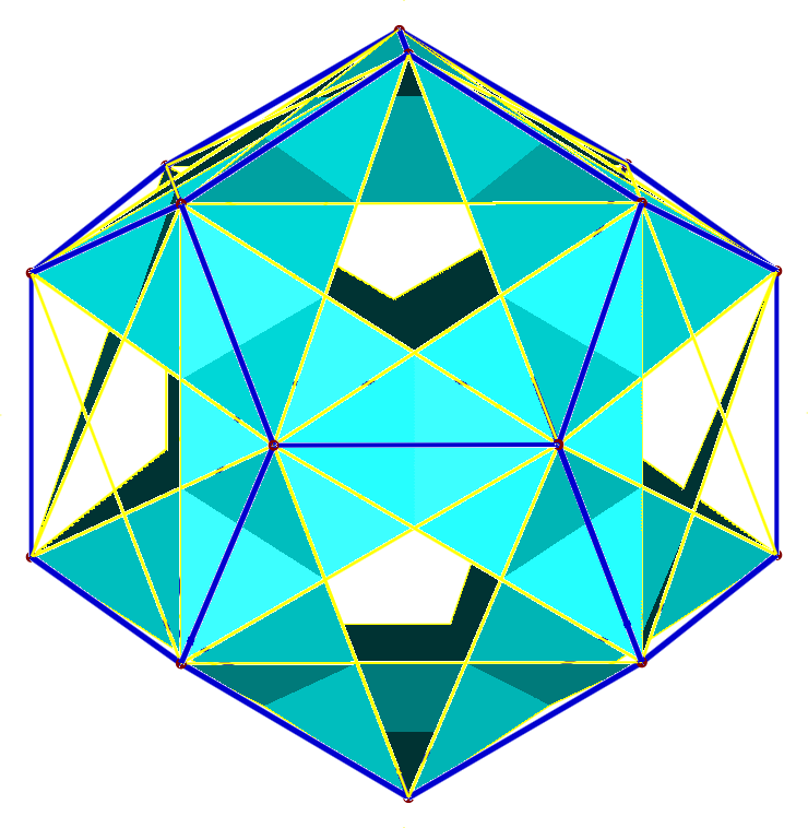
Figure 1: The $(20_{3})$ point-plane configuration obtained from the regular dodecahedron by the $V\!$-construction.

We conclude this section with the following example. Let $G$ be the the dodecahedron graph. Then $N(G)$ is a configuration $(20_{3})$. If $G$ is embedded in $\mathbb{E}^{3}$ as the 1-skeleton of the regular dodecahedron, then $N(G)$ is realized as a geometric point-plane configuration (see Figure 1).

We note that the same configuration is obtained by taking the 20 vertices and the planes spanned by the 20 triangular faces of either the small ditrigonal icosidodecahedron or the great ditrigonal icosidodecahedron (these polyhedra belong to the class of the 53 non-regular non-convex uniform polyhedra [11, 24]).

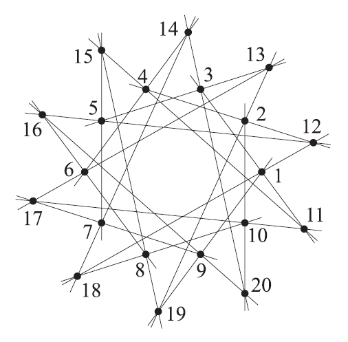
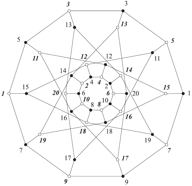
Figure 2: The flag-transitive triangle-free point-line configuration $(20_{3})$ (a), and its Levi graph (b).

On the other hand, we know that the Kronecker cover of the dodecahedron graph is isomorphic with the Levi graph of the $(20_{3})$ point-line configuration which is unique with the properties that it is triangle-free and flag-transitive [5] (Figure 2) (see also Figure 1 in [4]). Thus we can see that $N(G)$ can be realized geometrically as both a point-plane and a point-line configuration. As we show in the next section, a realization as a point-circle configuration may be of interest.

3 $V\!$-construction and configurations of points and circles.

In [16] it was observed that certain point-plane configurations obtained from a 3-polytope $P$ by the $V\!$-construction could also be realized by points and circles. A simple necessary condition for this is that for each vertex $v$ of $P$, the set of the first-neighbours of $v$ forms a concyclic set, i.e. one can draw a circle through its points. Moreover, such point-circle configurations can be carried over to the plane, using stereographic projection. Here the well-known property is used that the stereographic projection is a circle-preserving map, see for instance [25] (also [10, 23]).

Lemma 9.

Under stereographic projection from the sphere $S$ to the plane $\Sigma$ the image of any circle on $S$ is a circle on $\Sigma$.

A straightforward application of this leads to the following result.

Theorem 10.

Any point-circle configuration on the sphere gives rise to a planar point-circle configuration.

Here we explicitly state the result that is presented already in [16] (see Table 1 and 2 there), and follows readily from the above Theorem.

Corollary 11.

The $V\!$-construction of any Platonic or Archimedean polyhedron except for the octahedron gives rise to a planar point-circle configuration.

An example obtained from the regular dodecahedron is depicted in Figure 3. (Note that together with this, we have three distinct geometric realizations of one and the same abstract configuration of type $(20_{3})$; cf. Figures 1 and 2.)

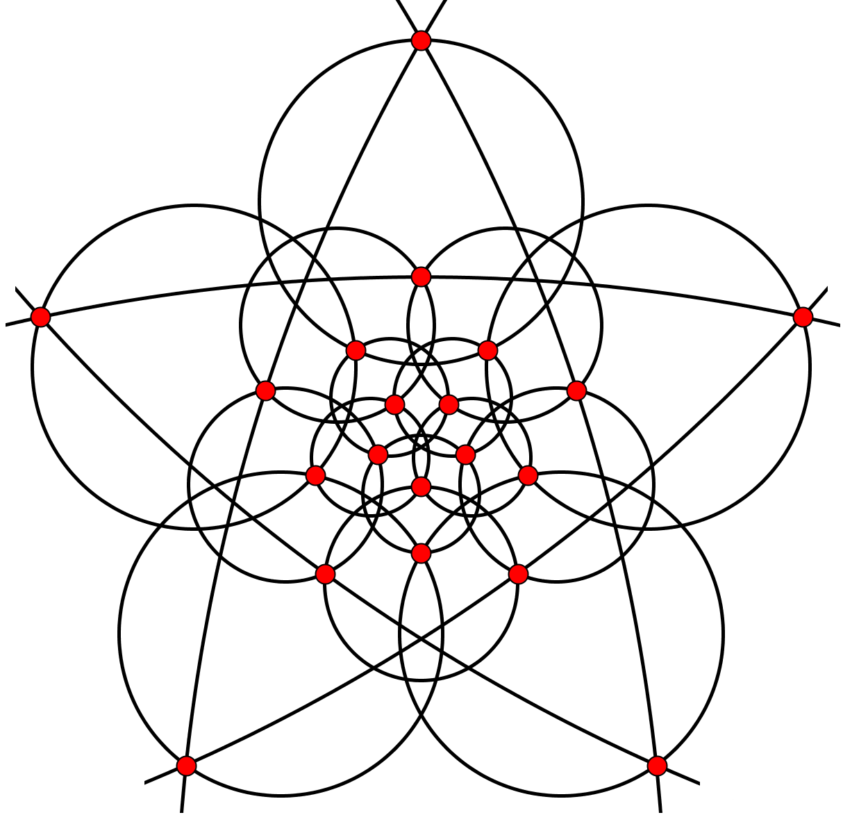
Figure 3: $(20_{3})$ point-circle configuration obtained from the regular dodecahedron by $V\!$-construction.

We remark that applying highly symmetric polytopes as a “scaffolding” for the construction of spatial point-line configurations is extensively used in [17].

In what follows we consider some other cases of $V\!$-construction that also give rise to planar point-circle configurations.

Proposition 12.

Any $(n_{3})$ configuration can be realized by points and circles in the plane.

Proof. We may place the $n$ points in the plane in general position, in such a way that no three lie on a line and no four lie on a circle. Obviously combinatorial lines can be realized by circles, and the combinatorial incidence is carried over to a geometric point-circle incidence. $\square$

The $(n_{3})$ point-circle configurations have an important property that is not shared by all point-circle configurations; namely, they are movable. To see this notion, we should consider that in the simplest case our point-circle configurations are constructed in the Euclidean plane $\mathbb{E}^{2}$. However, by adding to $\mathbb{E}^{2}$ a single point at infinity, we may consider them as lying in the inversive plane [10]. In this latter case, we say that a point-circle configuration is rigid if its geometric realizations form a single class under circle-preserving transformations.

We note that point-circle configurations can also be considered on the extended complex plane; in this case the circle-preserving transformations are just the Möbius transformations, i.e. fractional linear transformations [23]. Incidentally, they play an important role in the so-called Lombardi drawings of graphs, an idea not totally unrelated to point-circle configurations and studied by D. Eppstein and his co-workers, for instance in [12].

A configuration that is not rigid is called movable (cf. the notion of movability of point-line configurations, as defined in [21]). Having defined this notion, the following statement is straightforward.

Proposition 13.

Any $(n_{3})$ point-circle configuration is movable.

We note that movability is not a general property even for point-line configurations; for example, some classes of movable $(n_{4})$ configurations were discovered just recently [2, 3].

There is another property that distinguishes $(n_{3})$ point-circle configurations among all configurations. In general, the circles may be of different size. Let $r$ be the number of radii used in this construction. If $r=1$, all circles are of the same size, and the configuration is called an isometric point-circle configuration. It is not clear which $(n_{3})$ configurations can be realized as planar isometric point-circle configurations.

There is a large class of graphs that yields by V-construction isometric point-circle configurations in a natural way. These are the unit-distance graphs, i.e. graphs whose all edges have the same length (cf. [26, 27, 40]).

Theorem 14.

Let $G$ be a regular $d$-valent graph that is a unit-distance graph on $n$ vertices in the plane. Then $S(G)$ is an $(n_{d})$ configuration, realizable as an isometric point-circle configuration.

Proof. The points of the configuration are the vertices of the graph, as drawn in the plane. Unit-distance property implies that for each vertex, the set of its first-neighbours forms a concyclic set; furthermore, all these circles are of the same size. $\square$

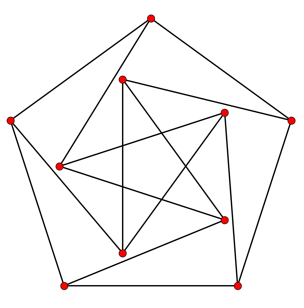
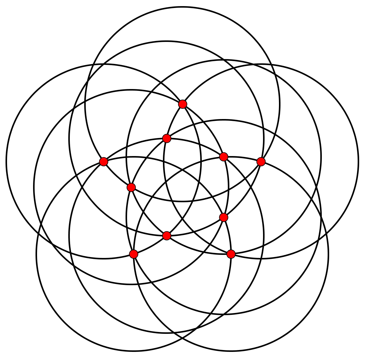
Figure 4: Applying the $V\!$-construction to a unit-distance representation of the Petersen graph (a) yields an isometric point-circle realization of Desargues’ configuration (b).

An interesting example is as follows. We know unit-distance representations of the Petersen graph [27, 40]; on the other hand, it is well known that the Kronecker cover of the Petersen graph is the Desargues graph [28] (which, in turn, is the Levi graph of the Desargues configuration [9]). Thus, on account of Theorem 3, the $V\!$-construction on a unit-distance representation of the Petersen graph yields an isometric point-circle realization of the Desargues configuration (see Figure 4).

We remark that the Desargues graph also has a unit-distance representation [40]. Thus one may also apply to it the $V\!$-construction, so as to obtain an isometric point-circle configuration. By our Corollary 8, this $(20_{3})$ configuration decomposes into two disjoint copies of the $(10_{3})$ Desargues point-circle configuration (see Figure 5, where the construction yields the two $(10_{3})$ copies in centrally symmetric position with respect to their common centre).

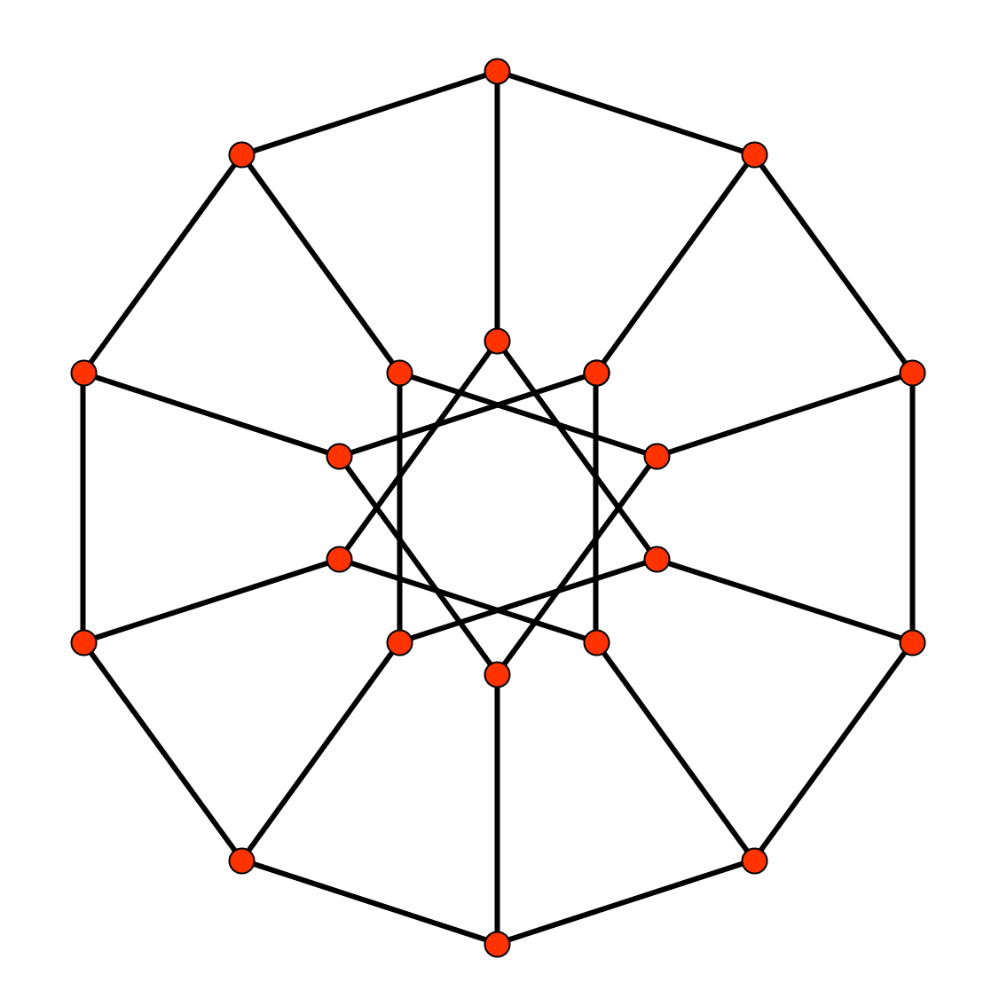
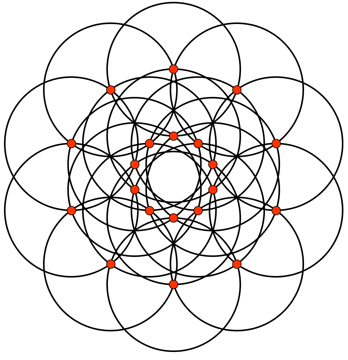
Figure 5: Applying the $V\!$-construction to a unit-distance representation of the Desargues graph (a) yields a configuration consisting of two disjoint copies of another isometric realization of the point-circle Desargues configuration (b). One of the two copies may be viewed in Figure 8.

4 $V\!$-construction on $d$-cubes and Clifford’s point-circle configurations

The particular case of the cube in Corollary 11 can be extended to the whole class of $d$-cubes. Because of its interesting connections, we discuss here the general case in some detail.

We recall that the infinite series of Clifford’s point-circle configurations is associated to his renowned chain of theorems. By Coxeter [9], these theorems can be formulated as follows.

Theorem 15 (Clifford’s chain of theorems).

 
(1) Let $\sigma_{1}$, $\sigma_{2}$, $\sigma_{3}$, $\sigma_{4}$ be four circles of general position through a point $S$. Let $S_{ij}$ be the second intersection of the circles $\sigma_{i}$ and $\sigma_{j}$. Let $\sigma_{ijk}$ denote the circle $S_{ij}S_{ik}S_{jk}$. Then the four circles $\sigma_{234}$, $\sigma_{134}$, $\sigma_{124}$, $\sigma_{123}$ all pass through one point $S_{1234}$.

(2) Let $\sigma_{5}$ be a fifth circle through $S$. Then the five points $S_{2345}$, $S_{1345}$, $S_{1245}$, $S_{1235}$, $S_{1234}$ all lie on one circle $\sigma_{12345}$.

(3) The six circles $\sigma_{23456}$, $\sigma_{13456}$, $\sigma_{12456}$, $\sigma_{12356}$, $\sigma_{12346}$, $\sigma_{12345}$ all pass through one point $S_{123456}$.

And so on.

We know the Levi graph of these configurations (Coxeter [9, 10]).

Lemma 16.

The Levi graph of the Clifford configuration of type $(2^{d-1}_{d})$ is isomorphic to the $d$-cube graph.

It turns out that our $V\!$-construction can be applied so as to obtain Clifford’s configurations.

Theorem 17.

The $V\!$-construction on a $d$-cube graph gives rise to an isometric $(2^{d}_{d})$ point-circle configuration in the plane. This configuration is disconnected and composed of two copies of isometric $(2^{d-1}_{d})$ point-circle configurations which are isomorphic to a member of the same type of Clifford’s infinite series of configurations.

Proof. The $d$-cube graph is the Cartesian product of $d$ edge graphs $K_{2}$. According to [26], it is a unit-distance graph. By Theorem 14, the $V\!$-construction applied on it gives rise to an isometric point-circle configuration $C$. Since the $d$-cube graph is bipartite, its Kronecker cover is composed of two disjoint isomorphic copies of the $d$-cube graph (by Proposition 1 in [28]). By Theorem 3, this Kronecker cover is the Levi graph of $C$. Since a configuration is uniquely determined by its Levi graph (by Lemma 2), it follows from Lemma 16 that $C$ is in fact composed of two disjoint copies of Clifford configurations of type $(2^{d-1}_{d})$. $\square$

Some smallest examples are depicted in Figures 6 and 7.

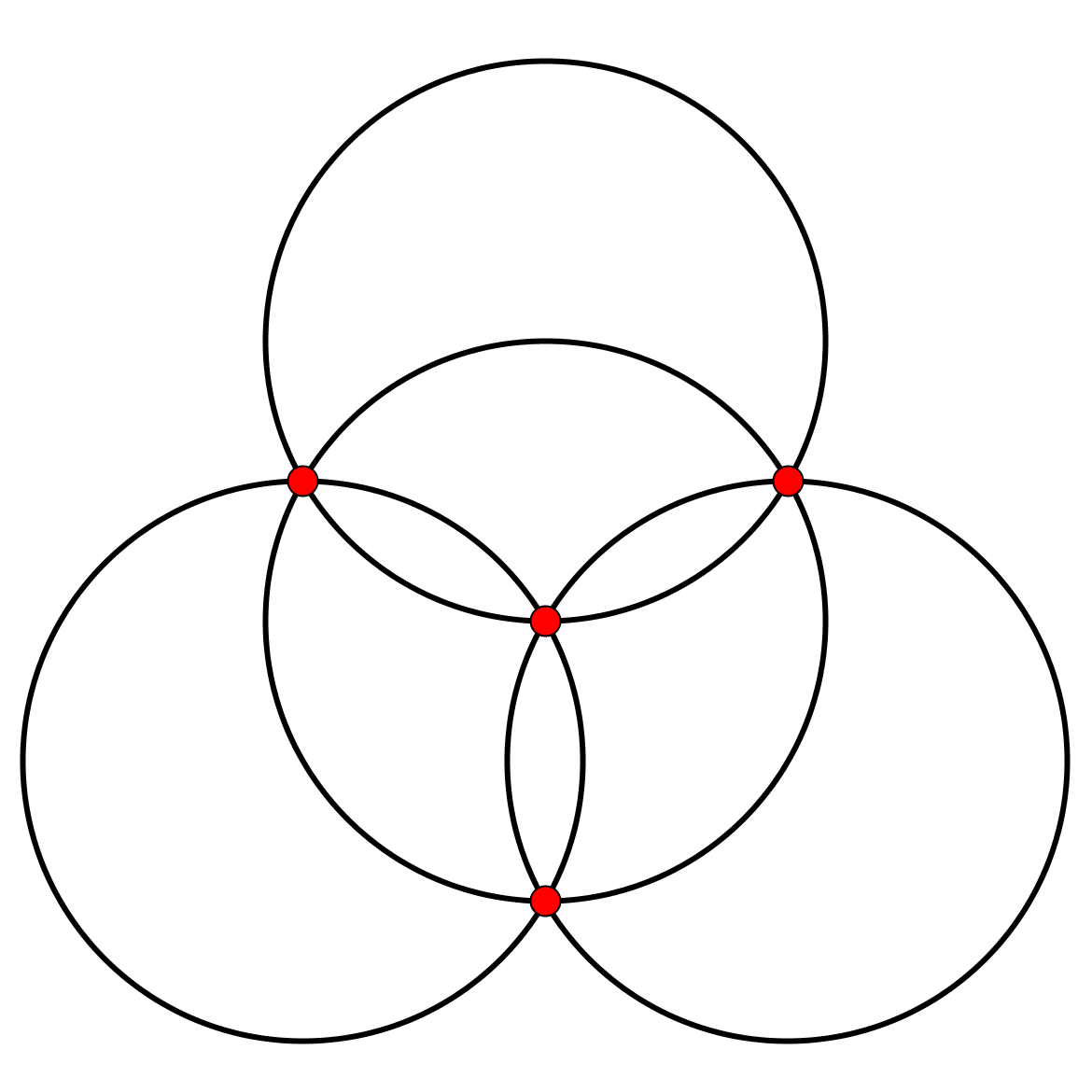
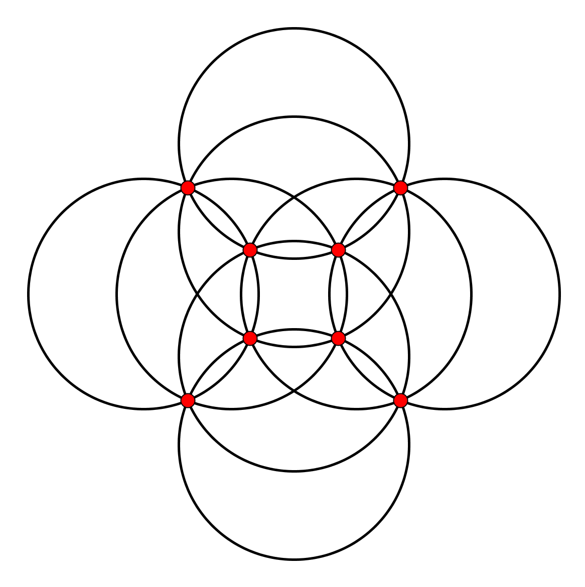
Figure 6: Isometric realization of Clifford configurations: $(4_{3})$ derived from the 3-cube graph (a), and $(8_{4})$ derived from the 4-cube graph (b).

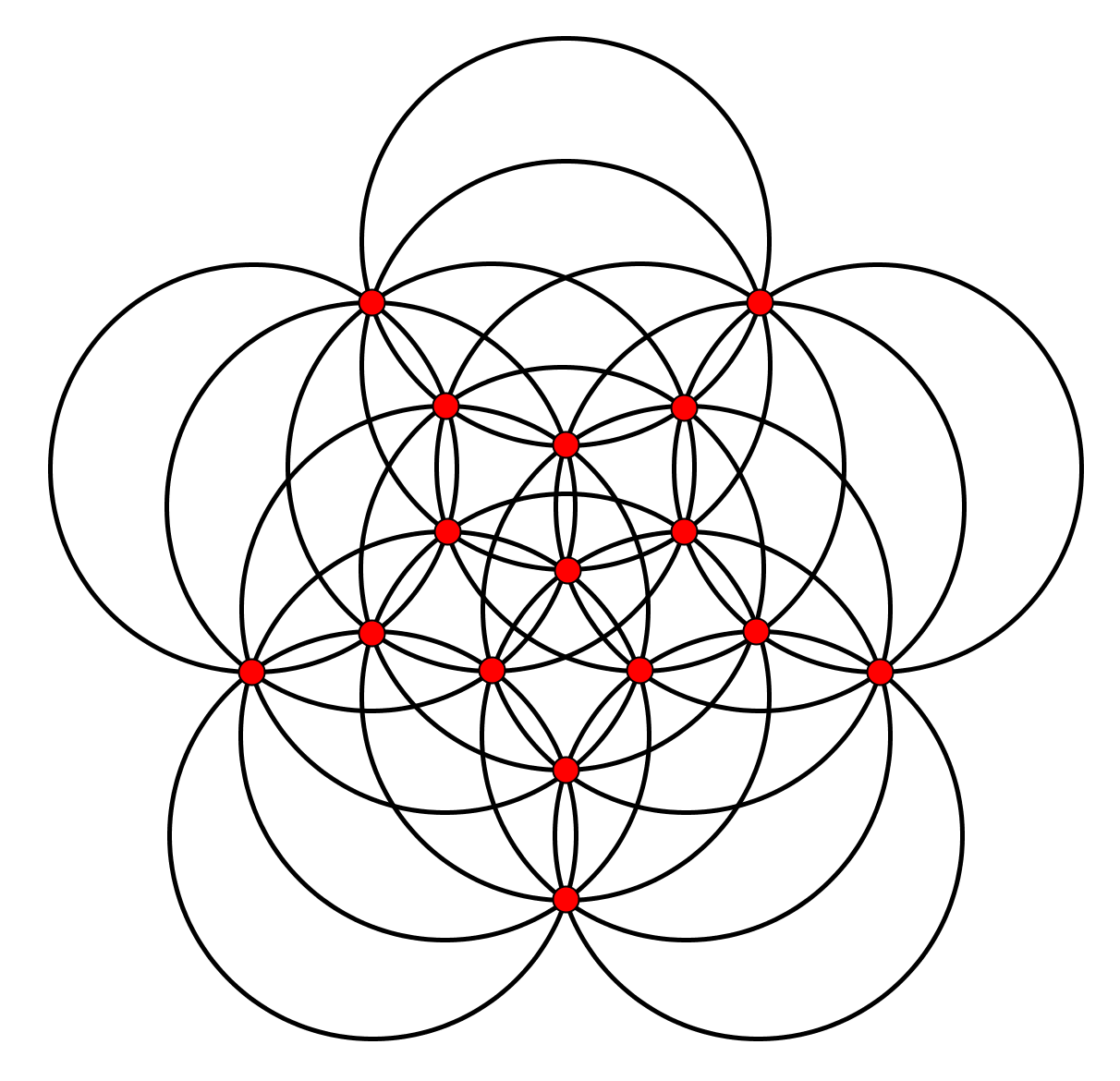
Figure 7: Isometric realization of Clifford’s configuration $(16_{5})$ derived from the 5-cube graph.

It is easy to see that the $d$-cube graph can be realized in the plane as a unit-distance graph in continuum many ways. In fact, take an arbitrary vertex and place it in the center of a unit circle. Its first-neighbours can be placed in different positions on the circle. Positions of the remaining vertices are then uniquely determined by sequences of rhombuses. This immediately gives the following corollary.

Corollary 18.

Every Clifford configuration is realizable as a movable isometric point-circle configuration.

Remark 19.

Realizability of Clifford’s configurations with circles of equal size is already known from [38] (see also [1]). Our approach provides an independent proof of this result.

5 Three new infinite classes of point-circle configurations

We start from the following observation. When applying the $V\!$-construction so as to obtain an isometric point-circle realization of Desargues’ configuration, the underlying Petersen graph need not be represented in unit-distance form. Indeed, compare our Figures 4 and 8. (We remark that the version depicted in Figure 8b is precisely the same as one of the components of the $(20_{3})$ configuration in Figure 5b.)

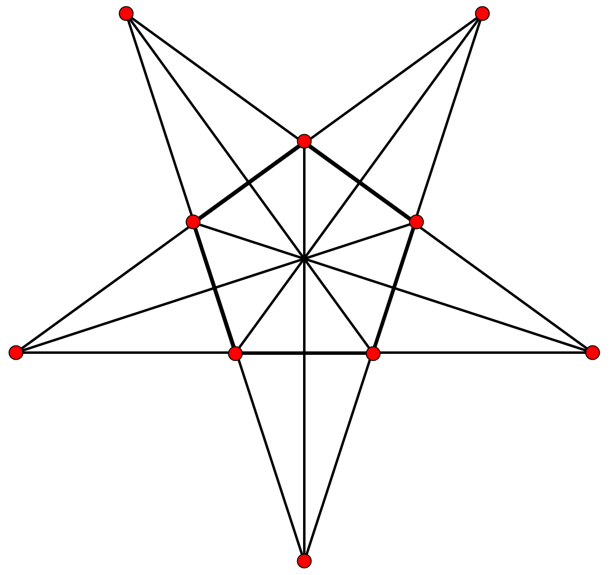
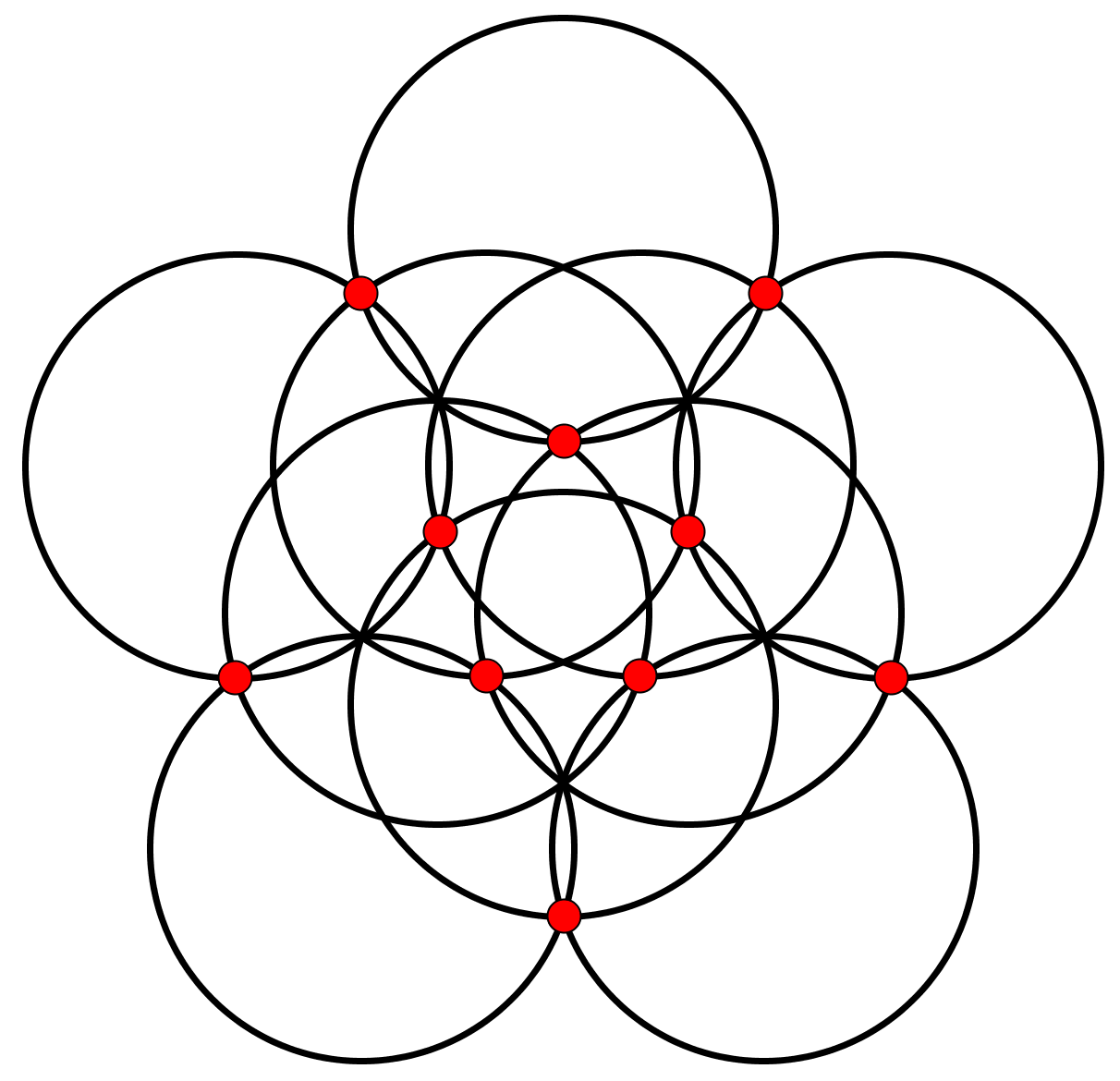
Figure 8: Isometric point-circle realization of Desargues’ configuration arising from a non-unit-distance representation of the Petersen graph. (Note that this is a degenerate representation in the sense that there are edges overlapping along the sides of the inner pentagon.)

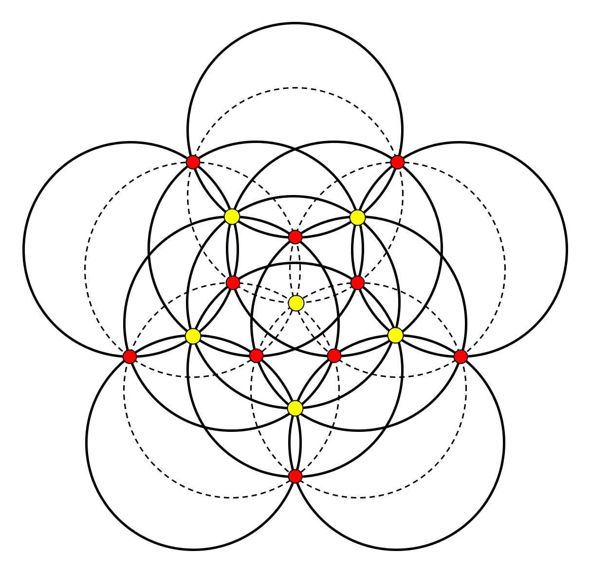
Figure 9: The Desargues point-circle configuration extended to the Clifford configuration $(16_{5})$.

Now Figure 8b suggests that this latter realization can be extended to a Clifford configuration of type $(16_{5})$. Figure 9 shows that such an extension is in fact possible (see also Figure 7). It turns out that this is a particular case of a more general relationship.

Before formulating it, recall that the Kneser graph $K(n,k)$ has as vertices the $k$-subsets of an $n$-element set, where two vertices are adjacent if the $k$-subsets are disjoint [19]. The Kneser graph $K(2n-1,n-1)$ is called an odd graph and is denoted by $O_{n}$. In particular, $O_{3}=K(5,2)$ is isomorphic to the Petersen graph. The bipartite Kneser graph $H(n,k)$ has as its bipartition sets the $k$- and $(n-k)$-subsets of an $n$-element set, respectively, and the adjacency is given by containment. Although the following relationship is well-known, we give a short proof of it.

Lemma 20.

The bipartite Kneser graph $H(n,k)$ is the Kronecker cover of the Kneser graph $K(n,k)$.

Proof. Let $A$ and $B$ be two $k$-subsets and let $A^{\prime}$ and $B^{\prime}$ be their respective $(n-k)$-complements. Clearly $A$ is adjacent to $B$ in $K(n,k)$ if and only if $A$ is adjacent to $B^{\prime}$ and $B$ is adjacent to $A^{\prime}$ in $H(n,k)$, and the result follows readily. $\square$

The bipartite Kneser graph $H(2n-1,n-1)$ is also known as the revolving door graph, or middle-levels graph; the latter name comes from the fact that it is a special subgraph of the $(2n-1)$-cube graph $Q_{2n-1}$ (considering $Q_{2n-1}$ as the Hasse diagram of the corresponding Boolean lattice) [35, 36]. It is a regular graph with degree $n$. Note that middle-levels graph is called a medial layer graph in [32] and is defined for any abstract polytope of odd rank.

Theorem 21.

For all $n\geq 3$, there exists an isometric point-circle configuration of type

$$\left(\dbinom{2n-1}{n-1}_{n}\,\right).$$

It is a subconfiguration of the Clifford configuration of type $\left(2^{2n-2}_{2n-1}\right)$. It can be obtained from the odd graph $O_{n}$ by $V\!$-construction.

Proof. Let $C$ be an incidence structure obtained from the odd graph $O_{n}$ by $V\!$-construction. By Theorem 3, the Levi graph of $C$ is the Kronecker cover of $O_{n}$. Lemma 20 implies that it is the bipartite Kneser graph $H(2n-1,n-1)$. Since this graph is a subgraph of the $(2n-1)$-cube graph $Q_{2n-1}$, from Lemma 2 follows that $C$ is isomorphic to a subconfiguration of the Clifford configuration of type $\left(2^{2n-2}_{2n-1}\right)$. Hence it can be realized as a planar point-circle configuration. The type of this configuration follows from the definition of $O_{n}$. Furthermore, Corollary 18 implies that this configuration also has an isometric realization. $\square$

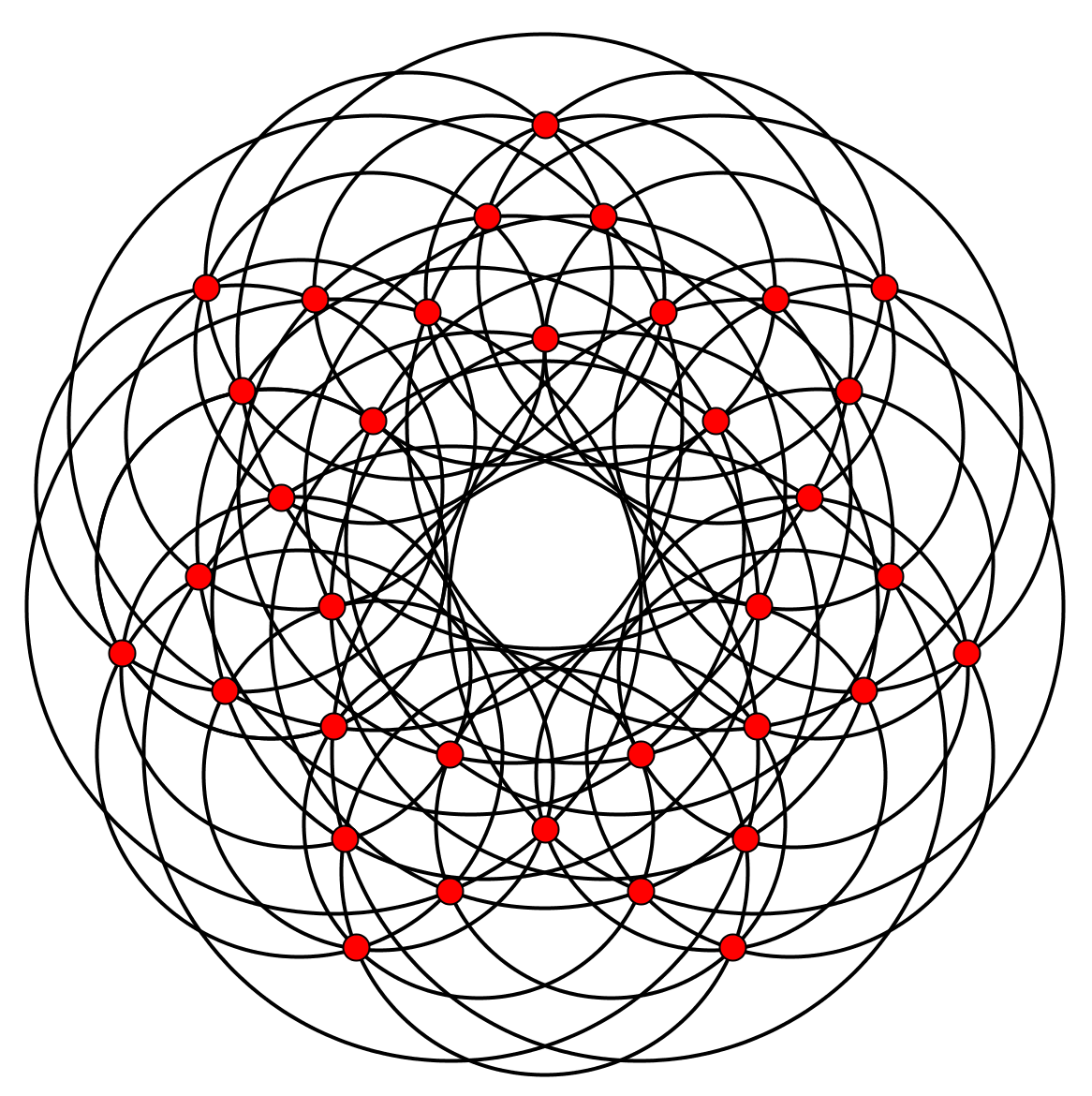
Figure 10: A point-circle realization of Danzer’s $(35_{4})$ configuration.

In the particular case of $n=4$ we have $(35_{4})$, which provides a point-circle realization of Danzer’s $(35_{4})$ point-line configuration (see Figure 10 for a non-isometric version). On this latter, Grünbaum wrote in 2008 [20]: “It seems that any representation of Danzer’s configuration is of necessity so cluttered and unhelpful for visualization that no attempt to present it has ever been made.” (see also [22]). We emphasize the geometric symmetry of this realization, which is the highest possible in the planar case; namely, $D_{7}$.

Our next new class also consists of isometric point-circle configurations.

Theorem 22.

For any $N$ and any $d>2$ there exists an isometric $(n_{d})$ point-circle configuration with $n>N$.

Proof. Take the Cartesian product of a long odd cycle $C_{N}$ and a $(d-2)$-dimensional cube graph. This is a unit-distance graph. Apply the $V\!$-construction to it. $\square$

Finally, we construct an infinite series of non-isometric $(n_{4})$ point-circle configurations. We start from a prism $P$ over an $n$-gon ($n\geq 3$) (the corresponding graph is also called a circular ladder). Then we take its medial $Me(P)$ [19, 33, 14], i.e. a new polyhedron such that its vertices are the midpoints of the original edges, and for each original vertex, the midpoints of the edges emanating from it are connected by new edges, forming a 3-cycle. In terms of solid geometry, the medial corresponds to a truncation of a right $n$-sided prism such that each truncating plane at a vertex is spanned by the midpoints of the edges incident with the given vertex (“deep vertex truncation”, see [39]). Note that in the particular case when the prism is the cube, its medial is the Archimedean solid called a cuboctahedron. Accordingly, we define the generalized cuboctahedron graph as the 1-skeleton of $Me(P)$, and denote it by $CO(n)$. Note that this graph can equivalently be defined as the line graph of the prism graph.

Observe that $CO(n)$ is an $4$-valent regular graph with $3n$ vertices. Moreover, it has a representation in the plane such that it exhibits the symmetry of a regular $n$-gon (thus its symmetry group is $D_{n}$); in this case its vertices lie on three concentric circles, $n$ vertices on each. It follows that the first-neighbour sets of the vertices are concyclic, hence the $V\!$-construction can be applied. Thus we obtain the following result.

Theorem 23.

For any $n\geq 3$, there exists a $((3n)_{4})$ point-circle configuration obtained from the generalized cuboctahedron graph $CO(n)$ by $V\!$-construction. It can be realized in the plane so that its symmetry group is the dihedral group $D_{n}$.

An example with $n=7$ is depicted in Figure 11. It is an open question if any member of the infinite series of these $((3n)_{4})$ configurations has an isometric realization.

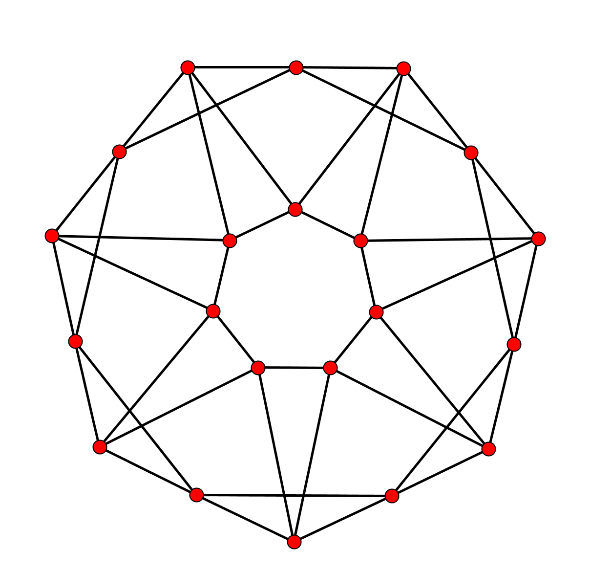
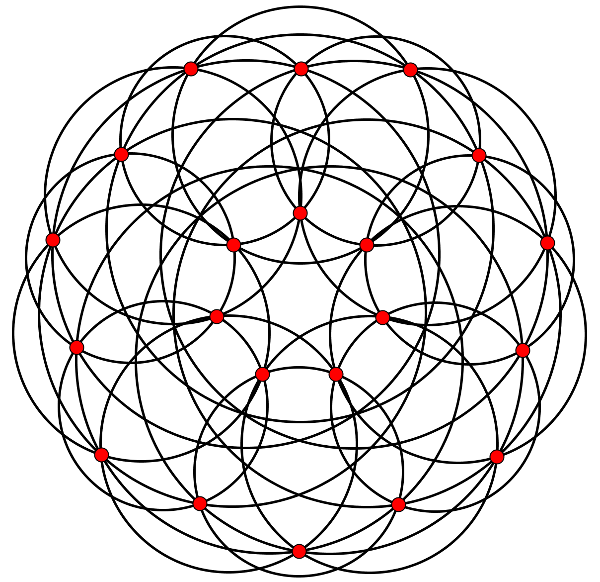
Figure 11: A representation of the generalized cuboctahedron graph with $D_{7}$ symmetry (a), and a $(21_{4})$ point-circle configuration obtained from it by $V\!$-construction (b).

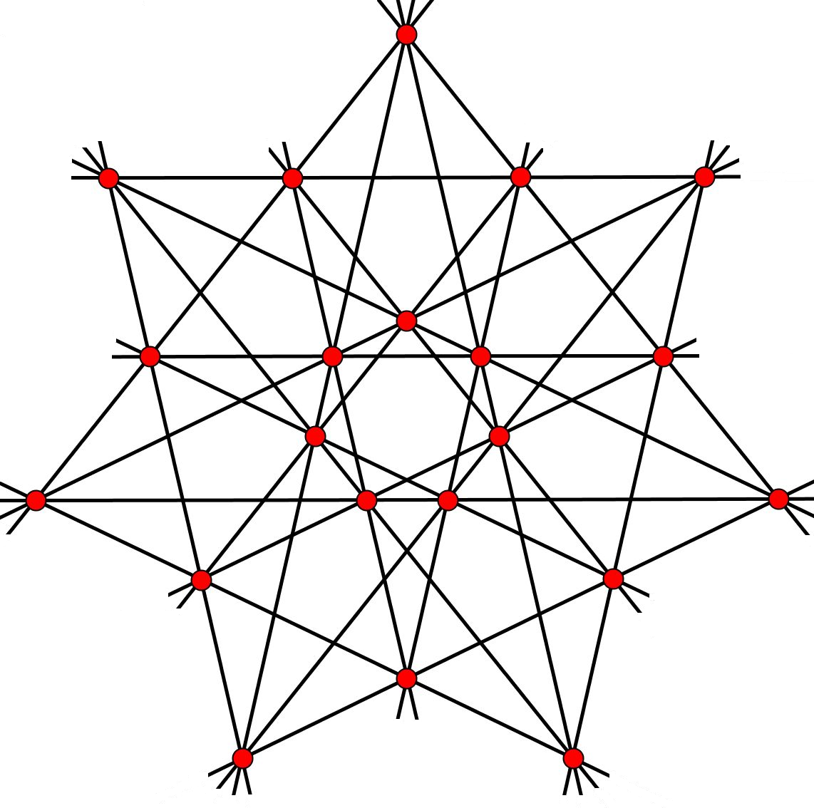
Figure 12: The point-line $(21_{4})$ configuration of Grünbaum and Rigby (a), one of its point-circle realizations with dihedral symmetry (b).

On the other hand, the mutual position of the points on the three orbits makes it possible to arrange the circles in several different ways, so as to obtain new, pairwise non-isomorphic $((3n)_{4})$ configurations. Here we do not investigate this possibility in detail. Instead, we just present an example, also of type $(21_{4})$ (non-isomorphic with the previous one), whose original point-line version is remarkable for several reasons (see Figure 12). We only mention here that it goes back to Felix Klein, 1879 (for further details, see [22]); on the other hand, its first graphic depiction only appeared in 1990 [20, 22]. This configuration also motivated the authors of [31] to present some geometric representations of a certain family of configurations that became later known as polycyclic configurations [6].

We note that several other already known families of graphs can serve as basis for obtaining new point-circle configurations by V-construction; just to mention some of them: generalized Petersen graphs [33], $I$-graphs [7]. In addition, the 1-skeleton of equivelar polyhedra is also a regular graph (see e.g. [18]); hence, finding suitable planar representations among them may also be promising in this respect.

6 Some comparisons beween different realizations of configurations

Comparing point-line and point-circle configurations, several questions arise, in particular, when different kinds of geometric realization of the same abstract configuration is considered. First we make the following conceptual distinction. Clearly, every point-line configuration can be transformed into a point-circle configuration by some suitable inversion. However, in this case, all the circles will have a common point (the inverse image of the point at infinity). To rule out this case, we use the term improper point-circle configuration. Accordingly, we call a point-circle configuration proper if its circles are not all incident with a common point. Clearly, all our examples presented in the previous sections are proper point-circle configurations. In what follows, we shall also speak about such configurations, and mostly omit the attribute “proper”.

A simple consequence of Proposition 12 is that by suitable displacement of the points, any planar ${n_{3}}$ point-line configuration can transformed into a point-circle configuration. For an incidence number larger than 3, it is more difficult to decide the existence of a point-circle representation of a point-line configuration.

Problem 24.

For $k\geq 4$, find an $(n_{k})$ point-line configuration which cannot be represented by a proper point-circle configuration.

The converse problem, in general, can also be quite difficult. However, here we know several examples. One of the oldest one is Miquel’s $(8_{3},6_{4})$ (for a simple proof why it has no point-line representation, see [34]). The infinite series of Clifford configurations also provides quite old, and balanced examples. In fact, since all the higher members contain, as a subconfiguration, the initial member of type $(4_{3})$, they cannot be represented by point-line configurations.

In the particular case of incidence number $k=4$, we have the following lower bound (a result of Bokowski and Schewe [8]).

Theorem 25.

For $n\leq 17$, there are no geometric point-line configurations $(n_{4})$.

As a consequence, consider e.g. the generalized Petersen graph $GP(n,r)$ [33]. For $n\leq 8$ it yields, by $V\!$-construction, a point-circle configuration which has no point-line representation.

In Section 3 we introduced the notion of an isometric point-circle configuration. We may impose two further conditions, which, together with the former, determine a particularly nice class of configurations. We call a point-circle configuration $\mathcal{C}$ lineal if two circles meet in at most one configuration points. Furthermore, $\mathcal{C}$ is called determining if the set of points of $\mathcal{C}$ coincides with the set of points in which more than two circles of $\mathcal{C}$ meet.

Note that these two conditions differ in the sense that the former determines a property on more abstract level, i.e. $\mathcal{C}$ is lineal if and only if it is isomorphic to a combinatorial configuration which is likewise lineal (we may call such a property of a geometric configuration intrinsic). On the other hand, the latter may depend on a particular representation of $\mathcal{C}$. For example, Figure 4b shows a determining representation of the Desargues configuration, while that in Figure 8b is non-determining. (Such a property may be called extrinsic; note that being isometric is another example of an extrinsic property in this sense.)

Now we call $\mathcal{C}$ perfect if it is lineal, isometric and determining. For example, the Desargues configuration in Figure 4b is perfect. A similar question can be posed for point-line configurations.

Problem 26.

Which configurations of points and lines can be realized as perfect point-circle configurations?

Geometric symmetry is also an interesting property which is worth investigating when different realizations of the same abstract configuration are compared. Are all symmetries of a point-line configuration realizable in its representation by points and circles? Of course, the converse question can also arise. Here we only mention that e.g. for the Pappus configuration not only its realization by lines can exhibit the maximal possible symmetry ($D_{3}$), but it can also be realized by circles with the same symmetry (see Figure 13).

On the other hand, it is a remarkable fact that while the Desargues configuration can be represented by points and lines with symmetry group either $C_{5}$ or $D_{5}$ (see Figures 4b and 8b, respectively), its classical point-line version can exist with neither of these symmetries. This follows from the theory developed in the paper [7] on $I$-graphs and the corresponding configurations. (We note that geometric realization of certain combinatorial objects with maximal symmetry is, in general, a problem which is far from trivial, see e.g. [15], and the references therein.)

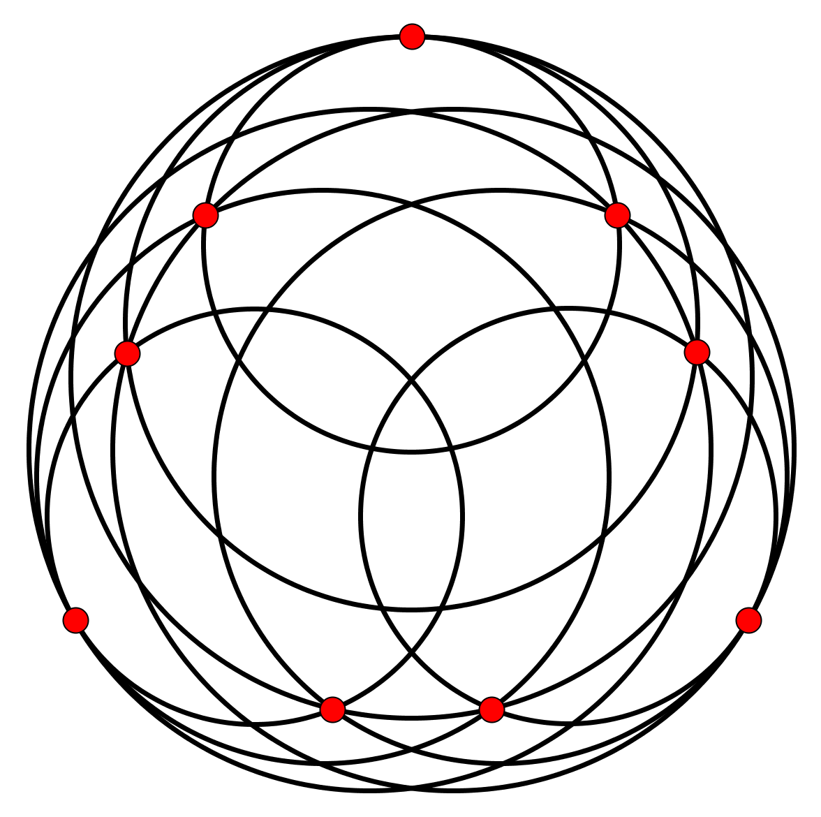
Figure 13: Two different realizations of Pappus’ configuration with symmetry $D_{3}$.

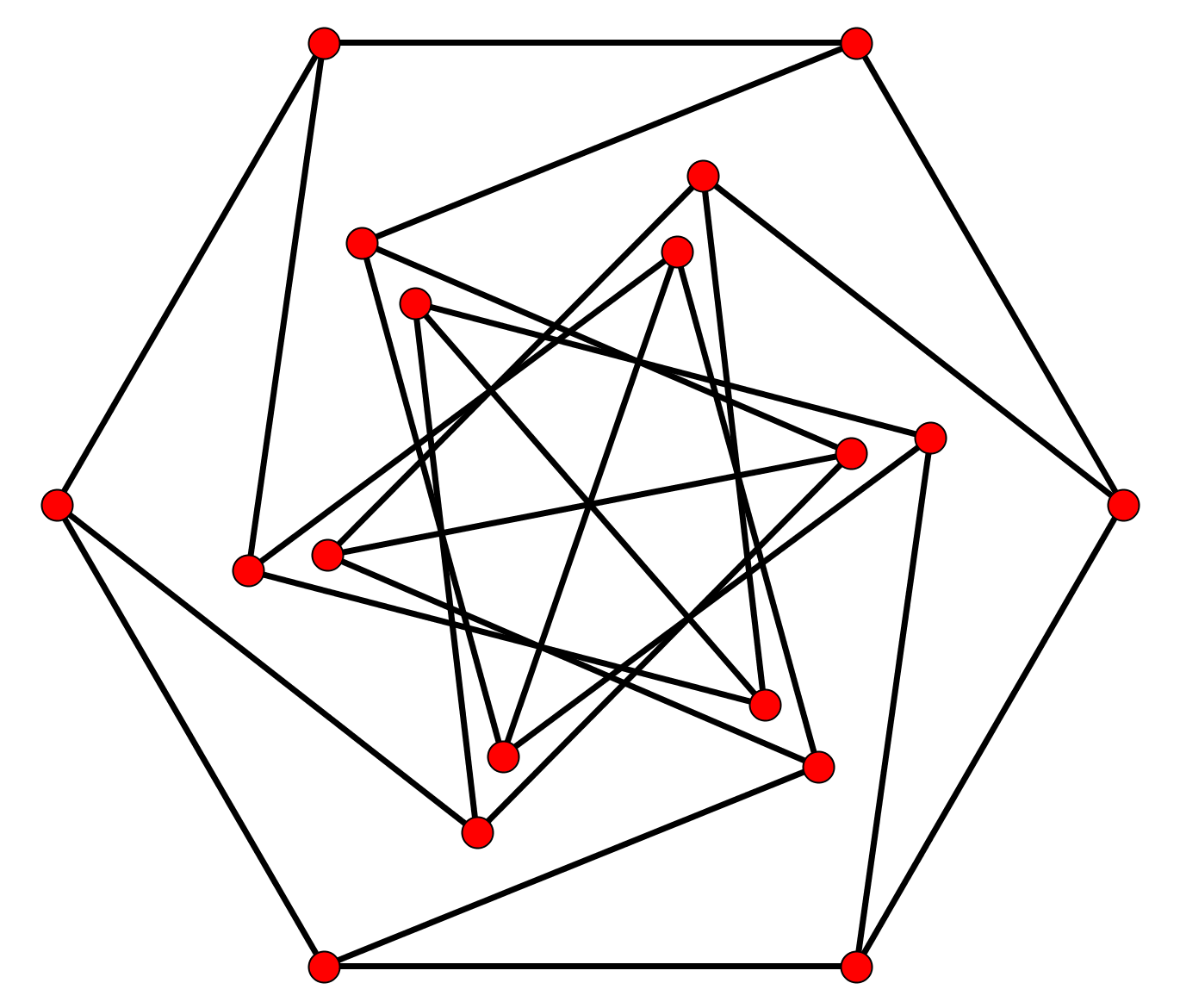
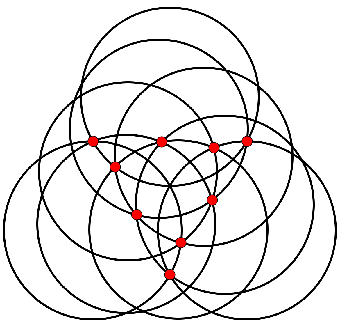
Figure 14: Unit-distance representation of the Pappus graph (a), and isometric point-circle representation of the Pappus configuration derived from it (b).

Considering point-circle realizations of the two oldest configurations, yet another difference occurs. Note that while Desargues’ configuration has a perfect realization (shown by Figure 4b), the realization of Pappus’ configuration shown by Figure 13b is not isometric (thus it is not perfect). On the other hand, when constructing an isometric representation, we find that it loses the property being determining (see the central triple crossing point in Figure 14b). This version is obtained from a unit-distance representation of the Pappus graph (see Figure 14a), using Corollary 8. Note that the symmetry reduces here to $C_{3}$ (for a representation of the Pappus graph with $D_{3}$ symmetry see e.g. [33], Figure 21).

References

- [1] D. W. Babbage, A chain of theorems for circles, Bull. London Math. Soc. 1 (1969), 343–344.
- [2] L. W. Berman, Movable configurations, Electron. J. Combin. 13 (2006), #R104.
- [3] L. W. Berman, J. Bokowski, B. Grünbaum and T. Pisanski, Geometric “floral” configurations, Can. Math. Bull. 52 (2009), 327–341.
- [4] A. Betten, G. Brinkmann and T. Pisanski, Counting symmetric configurations, Discrete Applied Math. 99 (2000), 331–338.
- [5] M. Boben, B. Grünbaum, T. Pisanski and A. Žitnik, Small triangle-free configurations of points and lines, Discrete Comput. Geom. 35 (2006), 405–427.
- [6] M. Boben and T. Pisanski, Polycyclic configurations, European J. Combin. 24 (2003), 431–457.
- [7] M. Boben, T. Pisanski and A. Žitnik, -graphs and the corresponding configurations, J. Comb. Des. 13 (2005) 406–424.
- [8] J. Bokowski and L. Schewe, On the finite set of missing geometric configurations , Comput. Geom. (in press)
- [9] H. S. M. Coxeter, Self-dual configurations and regular graphs, Bull. Amer. Math. Soc. 56 (1950), 413–455. Reprinted in: H. S. M. Coxeter, Twelve Geometric Essays, Southern Illinois University Press, Carbondale, 1968, 106–149.
- [10] H. S. M. Coxeter, Introduction to Geometry, Wiley, New York, 1961.
- [11] H. S. M. Coxeter, M. S. Longuet-Higgins and J. C. P. Miller, Uniform polyhedra, Phil. Trans. Roy. Soc. London Ser. A 246 (1954), 401–450.
- [12] C. A. Duncan, D. Eppstein, M. T. Goodrich, S. G. Kobourov and M. Nöllenburg, Lombardi drawings of graphs, J. Graph Algorithms Appl. 16 (2012), 37–83.
- [13] P. Erdős, F. Harary and W. T. Tutte, On the dimension of a graph, Mathematika 12 (1965) 118–122.
- [14] P. Fowler and T. Pisanski, Leapfrog transformations and polyhedra of Clar type, J. Chem. Soc. Faraday Trans. 90 (1994), 2865–2871.
- [15] G. Gévay, A class of cellulated spheres with non-polytopal symmetries, Canad. Math. Bull. 52 (2009), 366–379.
- [16] G. Gévay, Symmetric configurations and the different levels of their symmetry, Symmetry Cult. Sci. 20 (2009), 309–329.
- [17] G. Gévay, Constructions for large spatial point-line configurations, Ars Math. Contemp., to appear.
- [18] G. Gévay and J. M. Wills, On regular and equivelar Leonardo polyhedra, Ars Math. Contemp. 6 (2013), 1–11.
- [19] C. Godsil and G. Royle, Algebraic Graph Theory, Springer-Verlag, New York, 2001.
- [20] B. Grünbaum, Musings on an example of Danzer’s, European J. Combin. 29 (2008), 1910–1918.
- [21] B. Grünbaum, Configurations of Points and Lines, Graduate Texts in Mathematics, Vol. 103, American Mathematical Society, Providence, Rhode Island, 2009.
- [22] B. Grünbaum and J. F. Rigby, The real configuration , J. London Math. Soc. 41 (1990), 336–346.
- [23] L. Hahn, Complex Numbers and Geometry, The Mathematical Association of America, Washington, D. C. 1994.
- [24] Z. Har’El, Uniform solution for uniform polyhedra, Geom. Dedicata 47 (1993), 57–110.
- [25] D. Hilbert and S. Cohn-Vossen, Geometry and Imagination, Chelsea Publishing Company, NY 1952.
- [26] B. Horvat and T. Pisanski, Products of unit distance graphs, Discrete Math. 310 (2010), 1783–1792.
- [27] B. Horvat and T. Pisanski, Unit-distance representations of the Petersen graph in the plane, Ars Combin. 104 (2012), 393–415.
- [28] W. Imrich and T. Pisanski, Multiple Kronecker covering graphs, European J. Combin. 29 (2008), 1116–1122.
- [29] L. Klug, Az általános és négy különös Pascal-hatszög configuratiója (The Configuration of the General and Four Special Pascal Hexagons; in Hungarian), Ajtai K. Albert Könyvnyomdája, Kolozsvár, 1898. Reprinted in: L. Klug, Die Configuration Des Pascal’schen Sechseckes Im Allgemeinen Und in Vier Speciellen Fällen (German Edition), Nabu Press, 2010.
- [30] C. Lefèvre-Percsy, N. Percsy and D. Leemans, New geometries for finite groups and polytopes, Bull. Belg. Math. Soc. Simon Stevin 7 (2000), 583–610.
- [31] D. Marušič and T. Pisanski, Weakly flag-transitive configurations and half-arc-transitive graphs, European J. Combin. 20 (1999), 559–570.
- [32] B. Monson, T. Pisanski, E. Schulte and A. Ivić Weiss, Semisymmetric graphs from polytopes, J. Combin. Theory A 114 (2007) 421–435.
- [33] T. Pisanski and M. Randić, Bridges between geometry and graph theory, in C. A. Gorini (ed.), Geometry at Work, MAA Notes 53, Math. Assoc. America, Washington, DC, 2000, pp. 174–194.
- [34] T. Pisanski and B. Servatius, Configurations from a Graphical Viewpoint, Birkhäuser Advanced Texts Basler Lehrbücher Series, Birkhäuser Boston Inc., Boston, 2013.
- [35] J. J. Quinn and A. T. Benjamin, Strong chromatic index of subset graphs, J. Graph Theory 24 (1997), 267-273.
- [36] I. Shields, B. J. Shields and C. D. Savage, An update on the middle levels problem, Discrete Math. 309 (2009), 5271–5277.
- [37] H. Van Maldeghem, Slim and bislim geometries, in: A. Pasini (ed.) Topics in Diagram Geometry, Quaderni di Matematiche 12, Aracne, Roma, 2003, pp. 227–254.
- [38] P. Ziegenbein, Konfigurationen in der Kreisgeometrie, J. Reine Angew. Math. 183 (1940) 9–24.
- [39] G. M. Ziegler, Convex polytopes: extremal constructions and -vector shapes, in: E. Miller, V. Reiner and B. Sturmfels (eds.), Geometric Combinatorics, IAS/Park City Mathematics Series 15, American Mathematical Society – Institute for Advanced Study, 2007, pp. 617–691.
- [40] A. Žitnik, B. Horvat and T. Pisanski, All generalized Petersen graphs are unit-distance graphs J. Korean Math. Soc. 49 (2012), 475–491.