Transition to chaos and escape phenomenon in two degrees of freedom oscillator with a kinematic excitation

Abstract

We study the dynamics of a two-degrees-of-freedom (two DOF) nonlinear oscillator representing a quarter–car model excited by a road roughness profile. Modelling the road profile by means of a harmonic function we derive the Melnikov criterion for a system transition to chaos or escape. The analytically obtained estimations are confirmed by numerical simulations. To analyze the transient vibrations we used recurrences.

1 Introduction

The dynamics of a quarter-car model is governed by the road profile excitations and nonlinear suspension characteristics Verros2000 ; Gobbi2001 ; VonWagner2004 ; Litak2008a . These elements were discussed separately using simplified models and jointly by considering the more realistic description of a vehicle motion. For instance Verros et al Verros2000 proposed a quarter-car model with a piecewise linear dynamical characteristics. According to the adapted control strategy, the damping coefficient switched between two different values. Gobbi and Mastinu Gobbi2001 considered a two DOF model to derive a number of analytical formulae describing the dynamic behaviour of passively suspended vehicles running on randomly profiled roads. Their linear model approach was generalized by Von Wagner VonWagner2004 who determined a corresponding high-dimensional probability density by solving the Fokker-Planck equations. Finally, in papers Li2004 ; Litak2008a ; Naik2009 dynamics, bifurcations and appearance of chaotic solutions were discussed.

However the main issues of vehicle dynamics studies were unwanted and harmful vibration responses generated by vehicle as an effect of a rough surface road profile kinematic excitation Verros2000 ; Li2004 ; Turkay2005 ; Verros2005 ; Li2003 ; Shen2005 ; Yang2005a Thus the efficient reduction of them is still a subject of research among automotive manufacturers and research groups Genta2003 ; Andrzejewski2005 . Turkay and Akcay Turkay2005 considered constraints on the transfer functions from the road disturbance to the vertical acceleration, the suspension travel, and the tire deflection are derived for a quarter-car active suspension system using the vertical acceleration and/or the suspension travel measurements for feedback. The recent experimental and theoretical studies involved many new applications of active and semi-active control procedures Yang2005b ; Pan2005 ; Genta2003 ; Andrzejewski2005 ; Gao2004a . Consequently, previous mechanical quarter car models VonWagner2004 ; Shen2005 ; Yang2005a ; Andrzejewski2005 have been re-examined in the context of active damper applications. Dampers based on a magnetorheological fluid with typical hysteretic characteristics have a significant expectation for effective vibration damping in many applications Li2004 ; Gao2004b ; Yang2004 ; Litak2008b ; Siewe2010 ; Naik2011 ; Wu2011 ; Li2011 .

Recent efforts have been also focused on studies of the excitation of an automobile by a road surface profile with harmful noise components VonWagner2004 ; Litak2009a ; Borowiec2010 . Noise like chaotic vibrations, appearing due to the system nonlinearities, have been investigated in simplified single DOF models Li2004 ; Litak2008b ; Naik2009 . These papers follows the rich literature on an escape phenomenon in the symmetric and nonsymmetric Duffing or Helmholtz potentials Ciocogna1987 ; Szemplinska1988 ; Brunsden1989 ; Thompson1989 ; Bruhn1994 , where critical system parameters were determined. Note that the condition for escape could be applied as a criterion of fractality in basins of attraction and also as a transition to chaos Thomson1989. On the other hand, more sophisticated models of vehicle dynamics, namely half-car and full-car models, in the context of nonlinear response including chaotic solutions have been studied by Zhu and Ishitobi and also by Wang et al. Zhu2004 ; Zhu2006 ; Wang2010 .

To study a transition to the chaotic region and the corresponding critical parameters in low dimension dynamical system analytically, the Melnikov theory Melnikov1963 ; Guckenheimer1983 ; Wiggins1990 ; Seoane2010 ; Kwuimy2011 is often advocated. The application of this approach to a simple quarter-car model has been recently proposed by Li et al., and Litak et al. Li2004 ; Litak2008b . In the above papers, a single DOF model was used because of its simplicity. Consequently, the analytic consideration included also multiple scales analysis and harmonic balance Siewe2010 ; Borowiec2006 . The present paper is the continuation of the previous studies with an extension to a more realistic two DOF model, which includes the sprung and unsprung masses (Fig. 1).

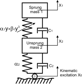
Figure 1: Two-degree-of-freedom quarter-car model ($y=x_{1}-x_{2}$).

Our article is organized in 4 sections. After introduction in the present section (Sec. 1) we present the model and discuss possibility of a global homoclinic bifurcation (Sec. 2). By the reduction of dimension we introduce the foundations of the Melnikov approach to the model. In this section (Sec. 2) we obtain the principal result as a critical curve which define the system parameters regions of regular and non-periodic (chaos, transient chaos or escape) behaviour. The simulation results, illustrating that transition results are also shown. Further results including recurrence analysis confirming the theoretical predictions are provided in Sec. 3. Finally in Sec. 4 we end up with conclusions and final remarks.

2 The model and global bifurcations

We start the analysis from the two DOF model presented in Fig. 1. The dynamics of vehicle excited by the road profile quarter car model is governed by nonlinear suspension characteristics. To examine a transition to the chaotic regime of vibrations, the Melnikov theory has been recently proposed Li2004 ; Litak2008b . In this perturbation approach the authors of previous works used a single DOF model.

In the present note we go beyond this assumption by considering an extension of a vehicle model with the defined unsprung and sprung masses (Fig. 1a). The differential equations of motion for both masses have the following form:

$$\frac{{\rm d}^{2}}{{\rm d}{\rm t}^{2}}x_{1}+\frac{c_{1}}{m_{1}}(\frac{{\rm d}}{\rm dt}x_{1}-\frac{{\rm d}}{\rm dt}x_{2})+\frac{\alpha_{1}}{m_{1}}(x_{1}-x_{2})$$ (1)

$$+\frac{\beta_{1}}{m_{1}}(x_{1}-x_{2})^{3}=0$$

$$\frac{{\rm d}^{2}}{{\rm d}{\rm t}^{2}}x_{2}+\frac{c_{2}}{m_{2}}(\frac{{\rm d}}{\rm dt}x_{2}-\frac{{\rm d}}{\rm dt}x_{0})-\frac{c_{1}}{m_{2}}(\frac{{\rm d}}{\rm dt}x_{1}-\frac{{\rm d}}{\rm dt}x_{2})$$ (2)

$$+\frac{\alpha_{2}}{m_{2}}(x_{2}-x_{0})-\frac{\alpha_{1}}{m_{2}}(x_{1}-x_{2})-\frac{\beta_{1}}{m_{2}}(x_{1}-x_{2})^{3}=0$$

where $m_{1}$, $m_{2}$ denote the corresponding sprung and unsprung masses (Fig. 1) $x_{0}=a\cos\omega t$ and describes the harmonic corrugation of a road profile. $c_{i}$, $\alpha_{i}$ (for $i=1$, 2) $\&$ $\beta_{1}$ are damping and stiffness coefficients, respectively.

Now we define the new variable $y=x_{1}-x_{2}$ of the relative motion:

$$\ddot{y}+\epsilon\frac{c_{1}}{m_{1}}\dot{y}+\frac{\alpha_{1}}{m_{1}}y+\frac{\beta_{1}}{m_{1}}y^{3}=\ddot{x}_{2}.$$ (3)

To adjust the above equations to application of the higher dimensional Melnikov approach Ruzziconi2011 ,the above equations can be approximated by introducing a small parameter $\epsilon$:

$$\ddot{y}+\epsilon\frac{c_{1}}{m_{1}}\dot{y}+\frac{\alpha_{1}}{m_{1}}y+\frac{\beta_{1}}{m_{1}}y^{3}=-\ddot{x}_{2}.$$ (4)

Consequently, the second equation (Eq. 2) gets the new form:

$$\ddot{x}_{2}+\frac{c_{2}}{m_{2}}\dot{x}_{2}+\frac{\alpha_{2}}{m_{2}}x_{2}=\frac{\alpha_{1}}{m_{2}}y+\frac{\beta_{1}}{m_{2}}y^{3}-\frac{c_{2}}{m_{2}}\omega a\epsilon\sin\omega t+\frac{\alpha_{2}}{m_{2}}a\epsilon\cos\omega t.$$ (5)

Using Melnikov approach Melnikov1963 for $y$ coordinate equation (Eq. 3) we study the Hamiltonian system of the nodal kinetic energy defined at the saddle points. In this way, time variability of $y$ and $\dot{y}$ are negligible. The above equations can be rewritten in the dimensionless form:

$$\ddot{y}+\epsilon C_{1}A_{1}\dot{y}+y+A_{3}y^{3}=-\ddot{x}_{2}.$$ (6)

$$\ddot{x}_{2}+C_{2}A_{1}\dot{x}_{2}+A_{2}Mx_{2}=C_{1}M\frac{\sqrt{m_{1}\alpha_{1}}}{m_{1}}\dot{y}+My+A_{3}My^{3}$$ (7)

$$-\epsilon C_{2}Ma\omega\sin(\omega t)+\epsilon A_{2}Ma\cos(\omega t),$$

where $C_{1}=\frac{c_{1}}{\alpha_{1}}$, $C_{2}=\frac{c_{2}}{\alpha_{1}}$, $A_{1}=\frac{\sqrt{\alpha_{1}}}{\sqrt{m_{1}}}$, $A_{2}=\frac{\alpha_{2}}{\alpha_{1}}$, $A_{3}=\frac{\beta_{1}}{\alpha_{1}}$, $M=\frac{m_{1}}{m_{2}}$ are dimensionless parameters. For further consideration we assumed that the system parameters are: $C_{1}=0.001$, $C_{2}=0.5$, $A_{1}=1$, $A_{2}=1$, $A_{3}=-16$, $M=5$. The excitation frequency and the corresponding amplitudes used in the analysis have been fixed to $\omega=1.5$, $a=0.08$ and $a=0.12$. In the numerical simulations we used the sampling time $\delta t=0.00418$.

To analyze a homoclinic bifurcation in the sprung mass vibration we make further approximation. The role of the small parameter $\epsilon$ is to determine the heteroclinic trajectory and decouple the equations of motion into separate equations for sprung and unsprung masses. Thus after above normalizations the equations can be expressed:

$$\dot{v}=-\epsilon C_{1}v-y-A_{3}y^{3}-\ddot{x}_{2},$$ (8)

$$\dot{y}=v,$$

$$\ddot{x}_{2}=-C_{2}\dot{x}_{2}-A_{2}Mx_{2}+M\left(C_{1}v+y+A_{3}y^{3}\right.$$ (9)

$$\left.-\epsilon C_{2}\omega a\sin\omega t+\epsilon A_{2}a\cos\omega t\right).$$

Interestingly, in the limit of small $\epsilon$ limit, $x_{2}$ can be approximated as:

$$x_{2} = \epsilon A\cos(\omega t+\phi-\psi)+x_{st}.$$ (10)

Note that in the above expression $x_{st}$, generated by slowly changing terms with $y$ and $\dot{y}$, is plating a role of the static displacement while $A$ as an amplitude.

Thus, the unperturbed equations (for $\epsilon=0$) can be obtained from the gradient of the unperturbed Hamiltonian $H^{0}(y,v)$:

$$\dot{y}=\frac{\partial H^{0}}{\partial v},\hskip 22.76228pt\dot{v}_{y}=-\frac{\partial H^{0}}{\partial y},$$ (11)

where $H^{0}$ is defined as follows:

$$H^{0}=\frac{v^{2}}{2}+V(y)$$ (12)

The corresponding effective potential is given by the expression:

$$V(y)=\frac{y^{2}}{2}+A_{3}\frac{y^{4}}{4}.$$ (13)

Following the standard Melnikov theory Melnikov1963 ; Guckenheimer1983 ; Wiggins1990 ; Seoane2010 ; Kwuimy2011 , we get the heteroclinic orbits connecting the two hyperbolic saddle points (coinciding with the maxima of the potential $V(y)$ (Eq. 12)): $y=\pm\sqrt{A_{3}^{-1}}$.

They can be expressed analytically as:

$$y^{*}=-\sqrt{A_{3}^{-1}}~{}\tanh\left[(t-t_{0})\frac{\sqrt{2A_{3}}}{2}\right],$$

$$v^{*}=\frac{{\rm d}y^{*}(t)}{{\rm d}t}=-\frac{\sqrt{2}}{2\cosh^{2}\left[(t-t_{0})\frac{\sqrt{2A_{3}}}{2}\right]}.$$ (14)

Figure 2: Potential of the restore force – $V(y)$ (Eq. 12) for different $A_{3}$ (a) and the corresponding heteroclinic orbits (b).

After perturbations the heteroclinic orbits the stable and unstable manifolds are calculated. Because of perturbations they are detracted (Fig. 3). As the characteristic distance between them $d\rightarrow 0$ the system possibilities of mixed solutions (regular and escape) appear which is equivalent to irregular chaotic and chaotic transient solutions. Thus $d=0$ is the ideal criterion for chaos appearance.

Figure 3: Stable and unstable manifolds of perturbed orbits terminated and started in the corresponding saddle points, and the distance between them $d$ (in $y-v$ plane).

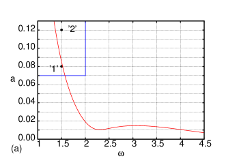
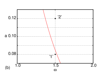
Figure 4: The Melnikov criterion, $a=\eta C_{1}$ versus $\omega$ for system parameters where $A_{3}=-16$, $M=5$, $A_{2}=1.5$, $C_{1}=0.001$ $C_{2}=0.5$. The curve separate the region of regular solutions (below the curve) from the chaotic and escape solutions (above the curve). Note that Fig. 4b magnifies the marked region in Fig. 4a, where the two indicated points symbolizes parameters used for numerical calculation points above and below the critical curve for $a=0.08$ at the point ’1’, and $a=0.12115$ at the point ’2’ ( $\omega=1.5$ for both cases).

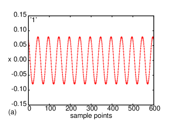
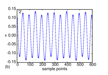
Figure 5: Time series (displacements of the sprung mass) of regular (a) a and irregular (or chaotic transient) (b) solutions for the same system parameters as in points ’1’ and ’2’ in Fig. 4a and b, respectively (the sampling time $\delta t=0.00418$). Note, the larger amplitude and additional modulation in (b).

Formally, the distance $d$ between perturbed stable and unstable manifolds are proportional to the Melnikov integral (Fig. 3) $d\sim\mathcal{M}(t_{0})$ Melnikov1963 ; Guckenheimer1983 ; Wiggins1990 which can be written:

$$\mathcal{M}(t_{0})=\int_{-\infty}^{+\infty}h\left(y^{*}(t),v^{*}(t)\right)\wedge g\left(y^{*}(t),v^{*}(t)\right){\rm d}t$$ (15)

where $\wedge$ denotes a wedge product, the differential form $h$ is the gradient of the unperturbed Hamiltonian and $g$ is related to the perturbation part, and $t_{0}$ is an integration constant. Both forms are defined on unperturbed heteroclinic orbit stable and unstable manifolds $W_{st(unst)}=(y_{st(unst)}^{*},v_{st(unst)}^{*})$.

$$h=v{\rm d}v+(-y-A_{3}y^{3}){\rm d}y$$ (16)

$$g=(A\omega^{2}\cos(\omega t+\phi-\Psi)-C_{1}v){\rm d}y.$$

Thus, after substitution the above forms to the Melnikov function $\mathcal{M}(t_{0})$ (Eq. 14) we get:

$$\mathcal{M}(t_{0})=M\int_{-\infty}^{\infty}\left(-C_{1}v^{*}+A\omega^{2}\cos(\omega t+\phi-\Psi)\right)v^{*}{\rm d}t$$ (17)

The condition for a global homoclinic transition, corresponding to a horse-shoe type of stable and unstable manifolds possible cross-section, can be written as:

$$\bigvee_{t_{0}}\mathcal{M}(t_{0})=0\hskip 42.67912pt{\rm and}\hskip 42.67912pt\frac{\partial\mathcal{M}(t_{0})}{\partial t_{0}}\neq 0.$$ (18)

Consequently, the critical parameter $\eta=a/C_{1}$ is now

$$\eta=\frac{2\sqrt{-A_{3}}}{3\pi\omega^{3}M}\sqrt{\frac{(A_{2}M-\omega^{2})^{2}+C_{2}^{2}\omega^{2}}{A_{2}^{2}+C_{2}^{2}\omega^{2}}}\sinh\left(\frac{\pi\omega}{\sqrt{-2A_{3}}}\right)$$ (19)

The results of the above analysis are presented in Fig. 4a. The curve separate the region of regular solutions from the chaotic and escape ones. The black points represents the parameters used for numerical simulations. To show this region of parameters Fig. 4b magnifies the surrounding area. The corresponding time histories are presented in Fig. 5a and b. Note that in purpose of simulations we used Eqs. 7–8 with $\epsilon=1$.

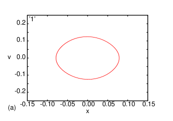
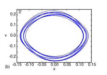
Figure 6: Phase portraits (displacements versus velocity of the sprung mass) of regular (a) and irregular (b) solutions for the same system parameters as point ’1’ and ’2’ in Fig. 4a and b, respectively.

Note that Fig. 5a shows the mono frequency while Fig. 5b more complex responses (multi-frequency or irregular). This is clearly visible in Fig. 6a and b where we show the corresponding phase diagrams. In Fig. 6a one can see a single line while in Fig. 6b lines are split into characteristic three lines patterns. It is worth to mention that the Melnikov criterion (Eq. 18 and Fig. 4) specifies the global transition associated with the destruction of borders between basins of attractions belonging to different solutions. In our case one of basin is related to escape from the potential well. The irregular solution denoted as no. 2 in Fig. 4, (see also Figs. 5b, 6b) must be related to such an escape. Really if someone continue the calculations for long enough time interval one observe the escape in the plot on time series (Fig. 7a) and on the phase portrait (Fig. 7b), respectively.

Focusing on the above solutions we discuss the recurrence properties of numerical results with more details in the next section.

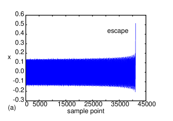
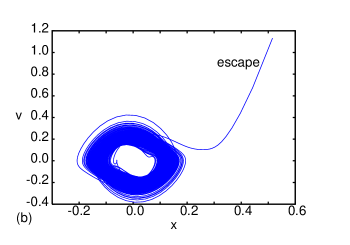
Figure 7: Time series of displacement (a) and phase portrait (b) during transient vibration escape (corresponding time interval $\Delta t=3844.25$, while sampling time $\delta t=0.00418$).

3 Recurrence plots analysis

The numerical solutions of the regular and transient nature can be analyzed more carefully by the recurrence plots. Eckmann1987 ; Casdagli1997 . This method is basing on the recurrences statistics and can be described by the matrix form ${\bf R}^{m,\epsilon}$ with corresponding 0 and 1 elements:

$$R_{ij}^{m,\varepsilon}=\Theta(\varepsilon-|{\bf x_{i}}-{\bf x_{j}}|)~{}~{}~{}{\rm for}~{}~{}~{}|i-j|\geq w~{}.$$ (20)

where ${\bf x_{i}}$ and ${\bf x_{j}}$ are usually defined in the embedding space of $m$ dimension and $\varepsilon$ is the threshold value. Here indices $i$ and $j$ denote the sampling instants. In our case we decided to use the $m=2$ and the embedding space includes the displacements of sprung and unsprung masses: $x_{j}=[y,x_{2}]$ (Eqs. 7–8 with $\epsilon=1$).

Having 0 and 1 values to be translated into the recurrence diagram as an empty place and a coloured dot respectively (see Fig. 9). Here $w$ denotes the Theiler window used to exclude identical and neighbouring points from the analysis Marwan2007 . Webber and Zbilut Webber1994 and later Marwan and collaborators Marwan2003 ; Marwan2007 developed the recurrence quantification analysis (RQA) for recurrence plots.

Shortly after invention $RQA$ were addressed to the biological and physiologic systems Webber1994 ; Marwan2008 . Recently this method has been applied for several technical systems Nichols2006 ; Litak2009b ; Litak2010 The first parameter of the RQA analysis defining the correlation function is the recurrence rate $RR$:

$$RR=\frac{1}{N^{2}}\sum_{i,j=1}^{N}R_{ij}^{m,\varepsilon},$$ (21)

which calculates the number of recurrences. In our case Theiler window $w=0$ in order to get the consistency with correlation sum Marwan2007 . In this language $\varepsilon$ expresses the correlation length of the characteristic sphere radius in the embedded space. Note that the correlation sum is the important tool which could be used to derive correlation dimension $D_{2}$. For small enough $\varepsilon$:

$$D_{2}=\frac{\log RR(\varepsilon)}{\log\varepsilon/\varepsilon_{0}}+const.,$$ (22)

where $\varepsilon_{0}$ is the arbitrary length.

Figure 8: The idea of states summation idea in the embedded space and the sphere of radius $\varepsilon$.

Furthermore the RQA can be used to identify topological structures of diagonal and vertical lines. In its frame RQA provides us with the probability $p(l)$ or $p(v)$ of line distribution according to their lengths $l$ or $v$ (for diagonal and vertical lines). Practically they are calculated

$$p(x)=\frac{P^{\varepsilon}(x)}{\sum_{x=x_{min}}^{N}P^{\varepsilon}(x)},$$ (23)

where $x=l$ or $v$ depending on diagonal or vertical structures in the specific recurrence diagram. $P^{\varepsilon}(x)$ denotes the unnormalized probability for a given threshold value $\varepsilon$. In this way Shannon information entropies ($L_{ENTR}$) can be defined for diagonal line collections

$$L_{ENTR}=-\sum_{l=l_{min}}^{N}p(l){\rm ln}p(l).$$ (24)

Other properties, such as determinism $DET$ and laminarity $LAM$:

$$DET=\frac{\sum_{l=l_{min}}^{N}lP^{\varepsilon}(l)}{\sum_{i,j=1}^{N}lP^{\varepsilon}(l)},$$ (25)

$$LAM=\frac{\sum_{v=v_{min}}^{N}vP^{\varepsilon}(v)}{\sum_{v=1}^{N}vP^{\varepsilon}(v)},$$

where $l_{min}$ and $v_{min}$ denotes minimal values which should be chosen for a specific dynamical system. In our calculations we have assumed $l_{min}=v_{min}=2$.

Table 1: Summary of recurrence quantification analysis (RQA) for $m=2$ and $\varepsilon=0.01$ for ’1’ and ’2’ solutions (see. Fig. 4-6).

type of
motion	$RR$	$DET$	$LAM$	$L_{ENTR}$
(’1’)	0.0348	1.0000	0.6078	1.3135
(’2’)	0.0080	0.9578	0.4743	1.7928

Determinism $DET$ is the measure of the predictability of the examined time series and gives the ratio of recurrent points formed in diagonals to all recurrent points. Note in a periodic system all points would be included in the lines. On the other hand laminarity $LAM$ is a similar measure which corresponds to points formed in vertical lines. This measure indicates the dynamics behind sampling point changes.

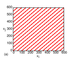
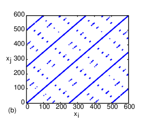
Figure 9: Recurrence plots for regular (a) and irregular (b) solutions for the same system parameters as point ’1’ and ’2’ in Fig. 4a and b, respectively ($\varepsilon=0.01$).

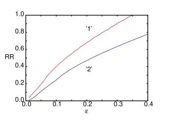
Figure 10: Recurrence rate $RR$ versus threshold value $\varepsilon$ for regular ’1’ and irregular ’2’ solutions (’1’ and ’2’ as Fig. 4a and b, respectively).

The results of our analysis calculated for time series ’1’ and ’2’ (see Fig. 4-6) are presented in Fig. 9 where we present the results of RP for $\varepsilon=0.01$. Note that both plots show regular features. However Fig. 9a is composed of full diagonals lines only, while in Fig. 9b each 5 line is full and between them one observes short line pieces or even insulated points. This would indicate multi-frequency modulated solution. Could be also a transient with basic regular and superimposed chaotic solutions. To shine this difference with more lights we show some estimated RQA parameters in Tab. 1. Obviously $RR$ is smaller for ’2’ (Fig. 9b) as we have broken lines instead of full ones (Fig. 9a). Moreover determinism and laminarity ($DET$ and $LAM$) are smaller smaller telling that that system is less regular. Consequently the more peculiar distribution of line lengths is confirmed by $L_{ENTR}$ which is larger for the solution ’2’. Additionally, in Fig. 10 we present the results of $RR$ versus $\epsilon$ (for relatively small $\epsilon$). One can see the significant difference between both solutions.

4 Summary and Conclusions

We have analyzed the two DOF quarter-car model, assuming that damping, suspension through the unsprung mass excited by the road profile corrugation can act as an perturbation on the main sprung mass. The obtained Melnikov criterion was latter confirmed by numerical simulations. The main conclusion coming from that point would be loss of stability of system appearing as the chaotic or transient chaotic or escape solution. The present investigation is going beyond research dealing with a single DOF quarter-car model Li2004 ; Yang2004 ; Litak2008b ; Litak2009a . In particular, the single DOF model assumes that the unsprung mass is significantly smaller than the sprung mass.

One should note that the model used in this paper, however more realistic than previous single-degree-of-freedom ones, is relatively simple and would not be sufficient to simulate the detailed response of a vehicle or compare to experimental results from real vehicles. Unfortunately, more sophisticated half-car and full-car models Zhu2004 ; Zhu2006 ; Wang2010 cannot be used in the frame of the presented approach as the heteroclinc trajectories could not be defined reliably. Furthermore, in higher DOF systems the analytic perturbation calculations are not possible.

However, the present quarter-car model is able to capture the major nonlinear effects that occur in vehicle dynamics and has demonstrated the transition to chaotic vibrations and synchronization phenomena Borowiec2010 ; Zhu2006 ; Borowiec2006 . Interestingly, the resulting critical amplitude curve (Fig. 4a, Eq. 19) has the maximum for $\omega\approx 3.1$ and the minimum for $\omega\approx 2.2$. The minimum is obviously related to the resonance region of the decoupled unsprung solution $x_{2}$ (Eqs. 8 and 9).

It should be also noted that the recurrence plots technique appeared to be very useful to study the transient signals. Thus the conclusions came from the analytic approach have been confirmed. Indeed, this method is designed for the short time series Marwan2007 ; Litak2010 Interestingly it also works for non-stationary signals Marwan2007 ; Litak2009b . The recurrences for RP and RQA analyzes have been obtain using the available commandline code written by Marwan Marwan . The recurence approach can be also used to higher DOF models of vehicle dynamics. The corresponding results on half and full vehicle models will reported in a separate paper.

References

- (1) G. Verros, S. Natsiavias, and G. Stepan, Control and dynamics of quarter-car models with dual-rate damping, J. Vib. Control 6, 1045–1063 (2000).
- (2) M. Gobbi and G. Mastinu, Analytical description and optimization of the dynamic behaviour of passively suspended road vehicles, J. Sound Vib. 245, 457–481 (2001).
- (3) U. Von Wagner, On non-linear stochastic dynamics of quarter car models, Int. J. Non-Linear Mech. 39 753–765 (2004).
- (4) S. Li, S. Yang, and W. Guo, Investigation on chaotic motion in histeretic non-linear suspension system with multi-frequency excitations, Mech. Res. Commun. 31, 229–236 (2004).
- (5) G. Litak, M. Borowiec, and R. Kasperek, Response of a magneto-rheological fluid damper subjected to periodic forcing in a high frequency limit, ZAMM–Z. Ang. Math. Mech. 88, 1000–1004 (2008).
- (6) R.D. Naik, P.M. Singru, Establishing the limiting conditions of operation of magneto-rheological fluid dampers in vehicle suspension systems, Mech. Res. Comm. 8, 957-962 (2009).
- (7) S. Turkay and H. Akcay, A study of random vibration characteristics of the quarter-car model, J. Sound Vib. 282, 111–124 (2005).
- (8) G. Verros, S. Natsiavas, and C. Papadimitriou, Design optimization of quarter-car models with passive and semi-active suspensions under random road excitation, J. Vib. Control 11, 581–606 (2005).
- (9) S. Li and S. Yang, Chaos in vehicle suspension system with hysteretic nonlinearity, J. Vib. Measure Diagnosis 23, 86-89 (2003).
- (10) Y. Shen, S. Yang, E. Chen and H. Xing, Dynamic analysis of a nonlinear system under semi-active control, J Vib. Eng. 18 219-222 (2005).
- (11) S. Yang, S. Li, and W. Guo, Chaotic motion in hysteretic nonlinear suspension system to random excitation, J. Vib. Measur. Diagnosis 25 22-25 (2005).
- (12) S. Yang, S. Li, X. Wang, F. Gordaninejad, and G. Hitchcock, A hysteresis model for magneto-rheological damper, Int. J Nonlinear Sci Numer. Simul. 6, 139-144 (2005).
- (13) C. Pan, S. Yang, and Y. Shen, An electro-mechanical coupling model of magnetorheological damper. Int. J. Nonlinear Sci. Numer. Simul. 6 69-74 (2005).
- (14) G. Genta, Motor Vehicle Dynamics (World Scientific, Singapore 2003).
- (15) R. Andrzejewski, J. Awrejcewicz, Nonlinear Dynamics of a Wheeled Vehicle (Springer, New York 2005).
- (16) G. Gao, S. Yang, E. Chen, and H. Xing, A study on the modeling of magnetorheological dampers for vehicle suspension based on experiment, Automobile Eng. 26, 683-685 (2004).
- (17) G. Gao, S. Yang, E. Chen, and J. Guo, One local bifurcation of nonlinear system based on magnetorheological dampers, Acta Mech Sinica 36, 564-568 (2004).
- (18) S. Yang, S. Li, Primary resonance reduction of a single-degree-of-freedom system using magnetorheological fluid dampers, J. Dyn. Control 2, 62–66 (2004).
- (19) G. Litak, M. Borowiec, M.I. Friswell, K. Szabelski, Chaotic vibration of a quarter-car model excited by the road surface profile, Commun. Non. Sci. Num. Sim. 13, 1373–1383 (2008).
- (20) M.S. Siewe, Resonance, stability and period-doubling bifurcation of a quarter-car model excited by the road surface profile, Phys. Lett. A 374, 1469–1476 (2010).
- (21) R.D. Naik, P.M. Singru, Resonance, stability and chaotic vibration of a quarter-car vehicle model with time-delay feedback, Commun. Non. Sci. Num. Sim. 16, 3397–3410 (2011)
- (22) C. Wu, W.-R. Wang, B.-H. Xu, X.-L. Li, W.-G. Jiang, Chaotic behavior of hysteretic suspension model excited by road surface profile, Journal of Zhejiang University (Engineering Science) 45, 1259–1264 (2011).
- (23) C. Li, S. Liang, Q. Zhu, Q Xiong, Analysis of chaotic vibration of a nonlinear quarter-vehicle model caused by the consecutive speed control humps, ICIC Express Letters 5, 3201-3207 (2011).
- (24) G. Litak, M. Borowiec, M.I. Friswell, W. Przystupa, Chaotic response of a quarter-car model excited by the road surface profile with a stochastic component, Chaos, Solitons & Fractals 39, 2448–2456 (2009).
- (25) M. Borowiec, J. Hunicz, A.K. Sen, G. Litak, G. Koszalka, and A. Niewczas, Vibrations of a vehicle excited by real road profiles, Forschung im Ingenieurwesen 74, 99–109 (2010).
- (26) G. Ciocogna, F. Popoff, Asymmetric duffing equation and the appearance of chaos. Europhys Lett 3 963–967 (1987).
- (27) W. Szemplinska-Stupnicka W. The refined approximate criterion for chaos in a two-state mechanical systems. Ingenieur Arch 58 554–566 (1988).
- (28) V. Brunsden, J. Coetell, P. Holmes, Power spectra of chaotic vibrations of a buckled beam. J Sound Vib 130 561–577 (1989).
- (29) J.M.T. Thompson, Chaotic phenomena triggering the escape from a potential well, Proc R. Soc. London A 421, 195–225 (1989).
- (30) Bruhn B, Koch BP, Schmidt G. On the onset of chaotic dynamics in asymmetric oscillators, Z. Angew. Math. Mech. 74 325–331 (1994).
- (31) Q. Zhu and M. Ishitobi, Chaos and bifurcations in a nonlinear vehicle model, J. Sound Vibr. 275, 1136-1146 (2004).
- (32) Q. Zhu and M. Ishitobi, Chaotic vibration of a nonlinear full-vehicle model, International Journal of Solids and Structures 43, 747–759 (2006).
- (33) W. Wang, G. Li and Y. Song Nonlinear dynamic analysis of the whole vehicle on bumpy road, Transactions of Tianjin University, 16 50–55.
- (34) V.K. Melnikov, On the stability of the center for time periodic perturbations, Trans. Moscow. Math. Soc. 12, 1-57 (1963).
- (35) J. Guckenheimer and P. Holmes, Nonlinear oscillations, dynamical systems and bifurcations of vectorfields (Springer, New York 1983).
- (36) S. Wiggins, Introduction to applied nonlinear dynamical systems and chaos (Spinger, New York 1990).
- (37) J.M. Seoane, S. Zambrano, I.P. Marino, M.A.F. Sanjuan, Basin boundary metamorphoses and phase control, Europhys. Lett. 90 30002 (2010).
- (38) C.A.K. Kwuimy, C. Nataraj, G. Litak, Melnikov’s criteria, parametric control of chaos, and stationary chaos occurrence in systems with asymmetric potential subjected to multiscale type excitation, Chaos 21, 043113 (2011).
- (39) M. Borowiec, G. Litak, and M.I. Friswell, Nonlinear response of an oscillator with a magneto-rheological damper subjected to external forcing, Applied Mechanics and Materials 5–6, 277–284 (2006).
- (40) L. Ruzziconi, G. Litak, S. Lenci, Nonlinear oscillations, transition to chaos and escape in the Duffing system with non-classical damping, Journal of Vibroengineering 13, 22–38 (2011).
- (41) J.-P. Eckmann, S. O. Kamphorst, and D. Ruelle, Recurrence plots of dynamical systems, Europhys. Lett. 5, 973–977 (1987).
- (42) M. C. Casdagli, Recurrence plots revisited, Physica D 108, 12–44 (1997).
- (43) N. Marwan, Encounters with neighbours: Current Development of Concepts Based on Recurrence Plots and their Applications, PhD Thesis (Universität Potsdam, Potsdam, 2003).
- (44) N. Marwan, M. C. Romano, M. Thiel, and J. Kurths, Recurrence plots for the analysis of complex systems, Phys. Rep. 438, 237–329 (2007).
- (45) C. L. Webber, Jr. and J. P. Zbilut, Dynamical assessment of physiological systems and states using recurrence plot strategies, J. App. Physiol. 76, 965–973 (1994).
- (46) N. Marwan, A historical review of recurrence plots, Eur. Phys. J. Spec. Topics. 164, 3–12 (2008).
- (47) J.M. Nichols, S.T. Trickey, and M. Seaver, Damage detection using multivariate recurrence quantification analysis, Mech. Syst. Signal Process. 20 421–437 (2006).
- (48) G. Litak, R. Longwic, Analysis of repeatability of diesel engine acceleration, Applied Thermal Engineering 29, 3574–3578 (2009).
- (49) G. Litak, M. Wiercigroch, B.W. Horton, and X. Xu, Transient chaotic behaviour versus periodic motion of a pendulum by recurrence plots, ZAMM- Zeit. Angewan. Math. Mech. 90, 33–41 (2010).
- (50) N. Marwan, Commandline Recurrence Plots, http:// www.agnld.uni-potsdam.de/ marwan/ 6.download/ rp.php (visited 2011-08-15).