Low angular momentum flow model for Sgr A*
Abstract
We examine the low angular momentum flow model for Sgr A* using two-dimensional hydrodynamical calculations based on the parameters of the specific angular momentum and total energy estimated in the recent analysis of stellar wind of nearby stars around Sgr A*. The accretion flow with the plausible parameters is non-stationary and an irregularly oscillating shock is formed in the inner region of a few tens to a hundred and sixty Schwarzschild radii. Due to the oscillating shock, the luminosity and the mass-outflow rate are modulated by several per cent to a factor of 5 and a factor of 2-7, respectively, on time-scales of an hour to ten days. The flows are highly advected and the radiative efficiency of the accreting matter into radiation is very low, –, and the input accretion rate yr-1 results in the observed luminosities erg s-1 of Sgr A* if a two-temperature model and the synchrotron emission are taken into account. The mass-outflow rate of the gas originating in the post-shock region increases with the increasing input specific angular momentum and ranges from a few to 99 per cent of the input accreting matter, depending on the input angular momentum. The oscillating shock is necessarily triggered if the specific angular momentum and the specific energy belong to or are located just nearby in the range of parameters responsible for a stationary shock in rotating inviscid and adiabatic accretion flow. The time variability may be relevant to the flare activity of Sgr A*.
keywords:
accretion, accretion discs – black hole physics – hydrodynamics – radiation mechanism: thermal – shock waves – Galaxy: centre.1 Introduction
Disc accretion is an essential process for such phenomena as energetic X-ray sources, active galactic nuclei and protostars. Since the early works by Pringle & Rees (1972) and Shakura & Sunyaev (1973), a great number of papers have been devoted to studies of the disc accretion onto gravitating objects. When the accretion rate is not too high, the accretion disc luminosity is directly in proportion to the accretion rate and can be successfully described by the standard thin disc model (S-S model). Sgr A* in our Galactic centre has been extensively studied in the category of accretion processes because it is a supermassive black hole candidate in our Galaxy and has unique observational features incompatible with the S-S model. One of the features of Sgr A* is that the observed luminosity is five orders of magnitude lower than that predicted by the S-S model. Moreover, the spectrum of Sgr A* differs from the multi-temperature black body spectrum obtained from the S-S model.
Since the observational features of Sgr A* can not be explained by the S-S model, two types of theoretical models, such as the spherical Bondi accretion model without any net angular momentum (Bondi, 1952) and the advection-dominated accretion flow model (ADAF) with high angular momentum (Narayan & Yi, 1994, 1995), have been proposed (Narayan & McClintock 2008, Yuan 2011 for review). Both the Bondi model and the ADAF model result in highly advected flows and the radiative efficiency is so low as to be compatible with the observations. The spherically symmetric Bondi model gave the first detailed model of Sgr A* (Melia, 1992; Melia, Liu & Coker, 2001). This model applies when the circularization radius is smaller than the innermost stable circular orbit. The Bondi model is frequently used to estimate the expected accretion rate near the Bondi radius far from the gravitating object. However, the simple Bondi model can not be extended close to the black hole to satisfy the details of the activity of Sgr A*. In contrast with the Bondi model, the ADAF model applies when the angular momentum at the outer boundary is roughly Keplerian, and a large fraction of the viscously generated heat is advected with the accreting gas and only a small fraction of the energy is radiated. Unlike the cold standard disc, this model results in a high temperature, rapid accretion, sub-Keplerian disc and inefficient radiation in the inner region of the disc. The ADAF models were shown to be generally successful and more advanced models (Yuan, Quataert & Narayan, 2003, 2004), taking into account the parametric description of the outflow and jet, explain well the observations. The important key to these models for Sgr A* is the amount of angular momentum in the accretion flow. However, at present, we have no clear evidence for the angular momentum from observations.
The low angular momentum model belongs to an intermediate case between the Bondi model and the ADAF model and was applied to Sgr A* (Mościbrodzka, Das & Czerny, 2006; Czerny & Mościbrodzka, 2008). Assuming that the Wolf-Rayet star 13 is the dominant source of the matter accreting onto Sgr A* and assuming the wind temperature = 1.0 or 0.5 keV, they estimated the net angular momentum of 1.68–2.16 and the Bernoulli constant of –, where the mass , the speed of light and the Schwarzschild radius are used as the units of mass, velocity and distance. With these flow parameters for and , they showed analytically that there is no continuous flow solution which attains to the event horizon, and the resulting flow would be non-stationary, but that, for the case of the angular momentum = 1.55 lower than the best estimates for Sgr A*, there exists a standard stationary shock solution. Subsequently, they speculated that, for the non-stationary flow, the inflowing matter accumulates and forms a ring or torus and that the ring in the inner region is unstable and may explain the variability of Sgr A*. Motivated by their suggestion and results, we examine the low angular momentum flow model for Sgr A* using 2D hydrodynamical calculations and discuss the results on the activity of Sgr A*.
2 Modelling a low angular momentum flow
We consider a supermassive black hole with mass for Sgr A*. For the accretion flow around Sgr A*, we use the flow parameters and estimated by Mościbrodzka, Das & Czerny (2006) and the mass accretion rate yr-1 in all models. 1D flow solution of a thin, rotating, inviscid and adiabatic accretion flow near the equatorial plane generally depends on the flow model especially on its thickness, for example, the vertical equilibrium model or the constant height model. Assuming the vertical equilibrium model here, we solve the Bernoulli equation with the constant angular momentum , find the outer and inner sonic points and get the Mach number versus radius relation, the sound speed , the thickness of the accretion flow, the radial velocity and the Temperature at a given radius (Chakrabarti, 1989). It should be noticed that the configuration of the Mach number versus radius does not coincide completely with that in Mościbrodzka, Das & Czerny (2006) because of the different flow model used. The Mach number versus radius relations for and 2.16 are similar to theirs, that is, the flow which passes through the outer sonic point never continue to the event horizon. The flow for also shows a flow topology similar to that for , unlike the case of Mościbrodzka, Das & Czerny (2006). The first purpose in this study is to examine how the flow with these specific angular momenta actually behaves. However, in addition to the above parameters, we examined another case of , for which the standing shock is predicted to exist in the inner region.
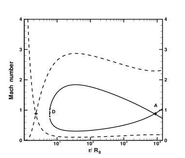
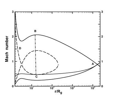
Figs 1 and 2 show the Mach number versus radius in 1D adiabatic flow obtained for the cases of = 1.68 and = (model A) and = 1.35 and = (model D), respectively. In Fig. 1, the particle which passes through the outer sonic point A falls down supersonically inward but never attains the event horizon since it makes a closed loop of the Mach number curve. On the other hand, in Fig. 2, the particle falls supersonically along the solid line AB, jumps at the shock position of from the point B to C in a subsonic state and tends supersonically toward the event horizon along the dashed line CD, where the Mach number curve (dashed line) which passes through the inner sonic point intersects at the point C with the other Mach number curve AC (dotted line) which passes through the outer sonic point and satisfies the Rankine-Hugoniot relation between the solid and the dashed lines. In Fig. 2, there exist two shock positions ( 17 and 19). It is known that usually the inner shock of the two shocks is unstable but the outer one is stable (Nakayama, 1994).
| model | |||||
|---|---|---|---|---|---|
| 1.68 | 3.97 | 1.6 | 4.0 | – | |
| 2.16 | 1.98 | 1.6 | 4.0 | – | |
| 1.55 | 1.98 | 1.6 | 4.0 | – | |
| 1.35 | 1.98 | 1.6 | 4.0 | – | |
| 1.68 | 3.97 | 1.6 | 4.0 | 3/7 | |
| 1.35 | 1.98 | 1.6 | 4.0 | 1/9 |
Thus far, the model parameters are listed in Table 1, where is the adiabatic index. First we examine models A–D using 2D radiation hydrodynamical calculations which include only the free-free transitions in the cooling and heating rate. It is well known that the existence of the sub-millimetre bump in Sgr A* spectra is certainly caused by the synchrotron emission. Secondly, following the results of models A and D, we examine another models of E and F which take account of the synchrotron cooling in the energy equation under an assumption that the magnetic energy density is 10 per cent of the thermal energy density. In models E and F, we adopt a two-temperature model where the ratio of the electron temperature to the ion temperature is initially assumed to be a constant and neglect the radiation transport because the flow is sufficiently optically thin and the flux-limitted diffusion approximation of radiation is less accurate for so optically thin medium.
3 Model equations
The set of relevant equations consists of six partial differential equations for density, momentum, and thermal and radiation energy. These equations include the heating and cooling of gas and radiation transport. The radiation transport is treated in the grey, flux-limited diffusion approximation (Levermore & Pomraning, 1981). We use spherical polar coordinates (,,), where is the radial distance, is the polar angle measured from the equatorial plane and is the azimuthal angle. The flow is assumed to be symmetrical with respect to the -axis () and the equatorial plane. In this coordinate system, we have the basic equations in the following conservative form (Kley, 1989):
| (1) |
| (2) |
| (3) |
| (4) |
| (5) |
and
| (6) |
where is the density, are the three velocity components, is the gravitational constant, is the gas pressure, is the specific internal energy of the gas, is the radiation energy density per unit volume, and is the radiation stress tensor. We adopt the pseudo-Newtonian potential (Paczyńsky & Wiita, 1980) in equation (2). The force density exerted by the radiation field is given by
| (7) |
where and denote the absorption and scattering coefficients and is the radiative flux in the comoving frame. The quantity describes the cooling and heating of the gas,
| (8) |
where is the source function. For this source function, we assume local thermal equilibrium , where is the gas temperature and is the radiation constant. For the equation of state, the gas pressure is given by the ideal gas law, , where is the mean molecular weight and is the gas constant. The temperature is proportional to the specific internal energy, , and satisfies the relation . To close the system of equations, we use the flux-limited diffusion approximation for the radiative flux:
| (9) |
and
| (10) |
where and are the flux-limiter and the Eddington Tensor, respectively, for which we use the approximate formula given in Kley (1989). The formula fulfills the correct limiting conditions in the optically thick diffusion limit, and as for the optically thin streaming limit.
In the two-temperature model with =0 for models E and F, the energy equation (5) is replaced by the following energy equations for ion and electron.
| (11) |
and
| (12) |
where and are the specific internal energy of the ion and electron, and are the ion and electron gas pressure, is the energy transfer rate from the ion to electron by Coulomb collisions, is the cooling rate by synchrotron radiation (Narayan & Yi, 1995), and = + .
4 Numerical methods
The set of partial differential equations (1)–(6) is numerically solved by a finite-difference method under adequate initial and boundary conditions. The numerical schemes used are basically the same as those previously described in Kley (1989) and Okuda, Fujita & Sakashita (1997). These methods are based on an explicit–implicit finite difference scheme. The inner boundary radius is taken to be . In our models, the outer shock will be formed in the region of if it exists. Therefore, the outer boundary radius is set to be 200 so that the predicted shock position never exceed the outer boundary. The computational domain is divided into grid cells, where grid points (=100) in the radial direction are spaced logarithmically as and grid points (=100) in the angular direction are equally spaced.
4.1 Initial flow variables
The initial flow variables in the 2D time-dependent calculation for models A–D are given from the 1D adiabatic flow mentioned in Section 2. To obtain the radiation energy density , we specify the ratio of the gas pressure to the total pressure and the Eddington factor . Then, the gas temperature and the radiation energy density are given by
| (13) |
and
| (14) |
Concerning , we specify its value so that the gas pressure is dominant and the temperature at the Bondi–Hoyle–Lyttleton radius () is comparable to the assumed wind temperature , where is given by the wind velocity 1000 s-1 and the wind temperature = 1.0 (Mościbrodzka, Das & Czerny, 2006). Consequently, and are adopted in all models. Table 2 shows the flow variables of the radial velocity , the Mach number , the density , the gas temperature , the radiation energy density , the relative thickness of the flow at the outer boundary , the radius of the outer sonic point and the gas temperature at the Bondi–Hoyle–Lyttleton radius.
On the other hand, as for the initial flow of models E and F, we use the final numerical results of models A and D, respectively and assume initially that and to maintain the pressure balance throughout the flow, where is the single temperature obtained from models A and D.
| Model | |||||||||
|---|---|---|---|---|---|---|---|---|---|
| ( | ( | ( | () | ( | () | ||||
| 4.75 | 1.91 | 5.86 | 2.45 | 8.86 | 0.45 | 8.359 | 9.5 | 9.6 | |
| 4.88 | 2.02 | 5.90 | 2.30 | 8.35 | 0.43 | 1.677 | 4.7 | 1.0 | |
| 4.95 | 2.06 | 5.83 | 2.28 | 8.20 | 0.43 | 1.681 | 4.7 | 1.0 | |
| 4.97 | 2.07 | 5.81 | 2.28 | 8.16 | 0.45 | 1.682 | 4.7 | 1.0 |
4.2 Initial and boundary conditions
At the outer boundary of the accretion flow, a continuous inflow with the flow variables in Table 2 is always given. The initial atmosphere above the accreting matter in the computational domain is given as a radially hydrostatic equilibrium state with zero azimuthal velocities everywhere. Physical variables at the inner boundary, except for the velocities, are given by extrapolation of the variables near the boundary. However, we impose limit conditions that the radial velocities are given by a free-fall velocity and the angular velocities are zero. On the rotational axis and the equatorial plane, the meridional tangential velocity is zero and all scalar variables must be symmetric relative to these axes. As for the outer boundary region above the outer accreting matter, we use free-floating conditions and allow for the outflow of matter, whereas here any inflow is prohibited. With these initial and boundary conditions, we perform time integration of equations (1)–(6) until a quasi-steady solution is obtained.
5 Numerical results
To get a steady state of flow, we need evolutionary times longer than the following dynamical time .
| (15) |
where is the angular velocity.
This time is a measure of the needed computational time. Actually, because unsteady shock phenomena occurred, we needed more times, of 5–7 , to examine the time variabilities, where s. The total luminosity is also a good measure to check whether a steady state of the accretion flow is attained. The luminosity is given by
| (16) |
5.1 Time variations of the luminosity and the mass–flow rate
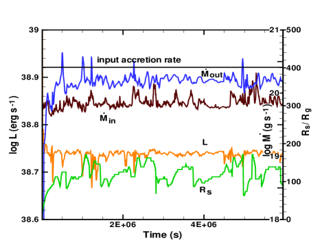
First, we show the results of model A as a typical case. After a time of , the total luminosity through the outer boundary nearly attains a steady value of but is modulated only by a few to ten per cent of the total luminosity. Following the time evolution of the flow, a shock wave is formed in the inner region of and it moves gradually outward. After a time of , the shock wave begins to oscillate irregularly between the radii of 80–160 with time-scales of hours to days. The mass-outflow rate at the outer boundary and the mass-inflow rate at the inner edge are modulated intermittently by a factor around 3. plus is nearly equal to the input accretion rate but it is remarkable that the mass-outflow rate is twice as large as the mass-inflow rate at the inner edge, that is, a large amount of the input accreting matter is ejected as a wind.
Fig. 3 shows the time variations of the total luminosity ( ), the mass-outflow rate ( ), the mass-inflow rate and the shock position on the equatorial plane for model A, where the input accretion rate is indicated by a dotted line and time is taken in units of seconds. The shock wave moves up and down over the spatial pre-shock zone, but it maintains the Mach number of 2 throughout the shock oscillation.
| Model | ( ) | |||||
|---|---|---|---|---|---|---|
| 5.4 | 0.32 | 0.68 | 80–160 | 1.04 | ||
| 5.3 | 1.0 | 0.99 | no shock | – | – | |
| 5.1 | 0.72 | 0.28 | 40–80 | 1.08 | ||
| 5.1 | 0.96 | 0.04 | 15–30 | 1.05 | ||
| 1.3 | 0.30 | 0.70 | 70–130 | |||
| 1.6 | 0.97 | 0.03 | 7–45 |
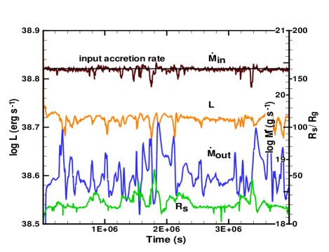
Although in model B with the highest the shock is formed firstly around and moves gradually upstream, it finally disappears and a steady flow is attained. In model C with smaller than model A, the flow features are similar to model A. But the shock oscillates between 40–80 and the mass-outflow rate varies by a factor of 4. Model D differs from the other models because the initial flow of model D is based on the 1D adiabatic flow with stationary standing shocks. Fig. 4 shows the time variations of , , and for model D. First, the shock is formed steadily at and it begins to move between 15 . The luminosity is modulated by several per cent but the mass-outflow rate varies by a factor of 7 although it is two orders of magnitude smaller than the input accretion rate. The Mach number of the shock maintains itself at about and is stronger than those in models A and C, because the shock is formed closer to the black hole.
We may wonder that the flow of model D shows non-stationary behaviours, because the initial flow of model D has been given from the adiabatic solution with the stationary standing shocks. So we examined this model under an adiabatic 2D condition and reconfirmed that the stationary shock is formed constantly at which is slightly smaller than the theoretical values of = 17 and 19 obtained from the 1D adiabatic solution. In model D, unlike the adiabatic case, we notice that the cooling and heating of the gas considerably influence the formation and position of the shock.
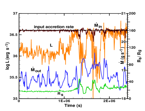
Fig. 5 shows the time variations of the total luminosity by the synchrotron and free-free emissions, , and for model F. The figure also shows the irregularly oscillating shock phenomena similar to model D but the modulation amplitude of the luminosity is much larger than that of model D and the maximum luminosity is as high as five times of the averaged luminosity erg s-1 which is comparable to the observed luminosity of Sgr A*. In the two-temperature models of E and F, the synchrotron emission is one orders of magnitude larger than the free-free emission and the energy transfer rate from the ion to electron by Coulomb collisions is negligibly small compared with the synchrotron emission.
Table 3 shows the averaged values of , and , the shock position on the equatorial plane, the maximum luminosity and the maximum mass-outflow rate , where is the input accretion rate of g s-1. The luminosities of the models A–D are independently of . The radiative efficiency of the accreting matter into the radiation is in models A–E but is far low, , in model F. The mass-outflow rate increases with increasing . In model B with the highest angular momentum, most of the input accreting matter is ejected as the wind, without arriving at the inner edge, and in model D with the lowest , only four per cent of the input matter is ejected as the wind. Conversely, the mass-inflow rate at the inner edge decreases as increases.
5.2 Structure of the flow and of the shock
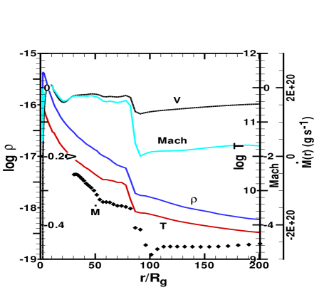
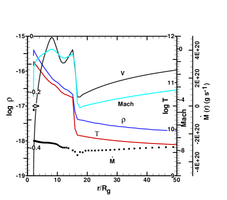
Fig. 6 shows the profiles of density (g ), gas temperature (), radial velocity , its Mach number on the equatorial plane and accreting mass flux (g s-1) versus radius at s for model A. The accreting mass flux is defined as the mass flux of the flow with negative radial velocities above the equatorial plane. Since the flow is convectively unstable in the inner region of , is not correctly defined at according to the above definition. The non-stationary shock is found at a radius of . The temperature at the outer boundary increases to at the pre-shock radius and is enhanced to across the shock. The density is also enhanced by a factor of three across the shock. In Fig. 6, a single shock structure is found but we find two shock features at some phases. The accreting matter falls inward with a constant accretion rate until it attains the shock position and then it decreases (see the scale on the right side of the figure) after the gas passes through the shock. This follows from the fact that the outflow begins in the post-shock region after matter crosses the shock. Fig. 7 shows the profiles of (g ), (), , its Mach number and (g s-1) at s for model D. The shock on the equatorial plane is found at . In this figure, we also find that the accreting mass flux becomes a little small in the post-shock region although it is almost constant until the gas reaches the shock. This is due to the effect of the mass-outflow in the post-shock region. However, the effect on the accreting mass flux is smaller than in model A, because the mass-outflow rate in model D is far smaller than in model A.
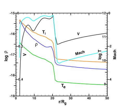
Fig. 8 shows the profiles of density (g ), ion temperature (), electron temperature (), radial velocity , Mach number of the velocity on the equatorial plane and accreting mass flux (g s-1) for model F at s, at which the luminosity takes a maximum value erg s-1. The profiles in the pre-shock region are almost same as the initial one and the ratio is not so different from its initial ratio even in the post-shock region. This means that the steady values of the electron and ion temperatures and accordingly the intrinsic total emission of models E and F may not be still reached by the time integration over s. To obtain exact steady distribution of and , the time-independent differential equations for a stationary state should be solved instead of the method of the time-dependent calculation. In spite of this fact, from the result of the two-temperature model with the input accretion rate of yr-1, we can expect the total emission of erg s-1 compatible with the observed one of Sgr A* if the electron temperatures of – K are obtained in the inner region.
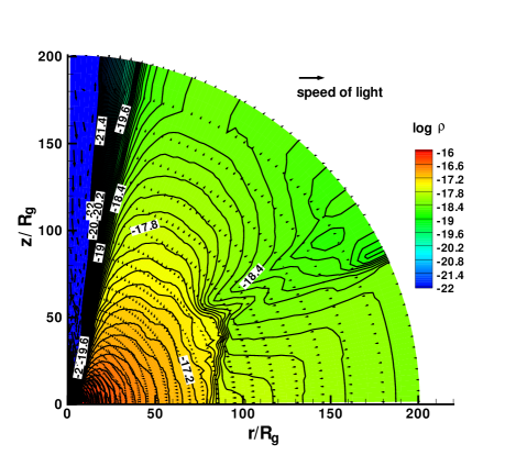
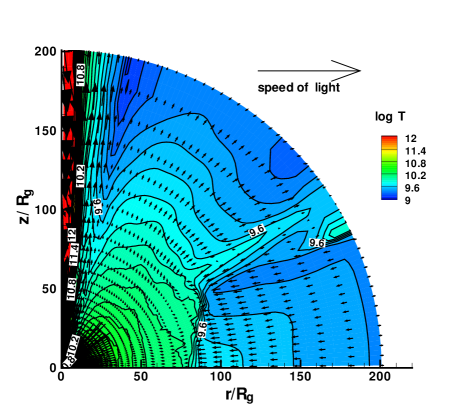
Figs 9 and 10 show the contours of density (g cm-3) and temperature (K) with velocity vectors at s in model A. The shock wave rises obliquely at above the equatorial plane and extends upward to . The velocity vectors in Fig. 10 are amplified by five times, compared with Fig. 9. The initial accreting matter at the outer boundary supersonically falls down towards the gravitating centre and is decelerated at the shock front, enhancing the density and the temperature and becomes subsonic. The post-shock region with high densities and high temperatures results in a strong outward pressure-gradient force also along the -axis and a part of the accreting matter deviates from the disc flow and escapes as the wind flow. The wind velocity becomes – at the outer boundary except for a narrow funnel region along the -axis, where the funnel wall is characterized by the vanishing of the effective potential and the flow velocity within the funnel region is relativistic at . The remaining accreting matter is swallowed into the central black hole. In model A, two thirds of the input accreting matter is expelled from the accretion flow. The mass-ouflow begins after the matter undergoes the shock compression. The circulating flow is also found at , that is, the accretion flow is convectively unstable in the post-shock region.
5.3 Properties of the time-variability of the flow
The most remarkable feature of the low angular momentum flow considered here is the existence of the non-stationary and oscillating shocks found in all models except for model B. This shock phenomenon results in the irregular modulation of the flow variable. .

The luminosity varies synchronously with the mass-outflow rate without any time lag. In spite of the large modulation of the shock position in models A, C, and D, the modulation amplitude of the luminosity is as small as a few to ten per cent , while in models E and F it varies by a factor of 2–5. The outflow consists of a persistent outflow and a large episodic one with irregular intervals of an hour to ten days and the episodic outflow rate is higher by a factor of 2–7 than the averaged mass-outflow rate.
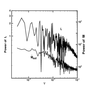
Sgr A* possesses a quiescent state and a flare state. The flares of Sgr A* have been detected in multiple wavebands from radio, sub-millimetre, IR to X-ray (Yusef-Zadeh et al., 2009, 2011). The amplitudes of the variability at radio, IR and X-ray are by factors of below 1/2, 1–5 and 45 or even higher, respectively, a few times per day. The rapid variability in the radio band on time-scales of a few seconds to hours has been observed (Yusef-Zadeh et al., 2011). Although a quasi-periodicity of 20 minutes in the IR flares (Genzel et al., 2003; Meyer et al., 2006a, b; Trippe et al., 2007; Eckart et al., 2008) and radio QPOs of 16, 22, 31 and 56 minutes (Miyoshi et al., 2011) have been reported, they are the subject of a controversy (Meyer et al., 2008; Do et al., 2009). These flare phenomena are interesting in relation to the time variations of the luminosity and the mass-outflow rate in the present models. We consider that the intermittently large modulations of the outflow due to the oscillatory shock may be related to the flares of Sgr A*. Unfortunately, the time resolution in our calculations is at most as small as a few minutes because of the limited time step in the calculations. Therefore, the short time variability at a scale of 10 minutes observed in Sgr A* can not be compared with the result of our models. Figs 11 and 12 show the power spectrum density of the total luminosity and mass-outflow rate and of the disc luminosity and shock radius on the equatorial plane, respectively, for model A, where the disc luminosity is defined at the surface of the inward flow with only negative radial velocities near the equatorial plane. Here, we can not find a conspicuous frequency peak in these power spectra partly due to insufficient statistical power but they are suggestive of semi-regular variabilities on time-scales of hours to days.
The origin of the oscillating shock appearing in the present models is entirely attributed to the range of parameters of the specific energy and the specific angular momentum used here. Generally, the shock formation and its position are very sensitive to the upstream flow parameters. The initial flow variables of the models, except for models D and F with , are based on the 1D adiabatic flow in which parameters never produce a stationary standing shock but are located just nearby in the range of parameters responsible for the stationary shock. Furthermore, we know that the shock becomes unstable when we take account of the energy loss and gain of the gas (Molteni et al., 1996; Okuda et al., 2004).
6 Comparison with the advection-dominated accretion flow
The present low angular momentum flow models are compared with the ADAF model (Narayan & Yi, 1994, 1995; Narayan & McClintock, 2008; Yuan, Quataert & Narayan, 2003) which is referred to as a radiatively inefficient accretion flow model of Sgr A. The region considered here is limited to an inner region of . The ADAF has generally the following properties: (1) the accretion flow becomes geometrically thick, (2) the pressure support in the radial direction is considerable, so the angular velocity is sub-Keplerian, (3) the radial velocity of the gas is much larger than that of the standard disc model and is barely less than Keplerian velocity in the innermost region, and (4) the large radial velocity and the large scale height cause the gas density to be very low, and so the cooling time is very long compared with the dynamical time and the matter is optically thin. These properties are also realized in the present low angular momentum flows. The ADAF solution is gas-pressure dominated and the sound velocity is comparable to the Keplerian velocity, so the gas temperature becomes nearly virial. Gas at such a high temperature radiates copiously at small radii where the temperature can approach . Thus, in the ADAF model, a two-temperature plasma of the ion temperature and the electron temperature is assumed to exist at the small radii. Typical ADAF models have the two temperatures scaling as (Narayan & McClintock, 2008)
| (17) |
In our models A–D, the two-temperature model is not considered but a high temperature of K comparable to the above ion temperature is obtained in the innermost region. The temperature profile is roughly in all models, in agreement with the ADAF. In the ADAF with the constant accretion rate, a self-similar flow with the density profile of gives , while our models show –. The radiative efficiency of the accretion flow in our model F is as small as in the usual ADAFs.
Thus, as far as the inner region of the accretion flow is concerned, the low angular momentum flow model has many properties in common with those of the ADAFs. The distinction between the ADAFs and the present low angular momentum flow is that the former describes a hot, nearly spherical, accretion flow with viscosity, while the latter shows the same accretion flow with lower angular momentum but without viscosity. The remarkable difference between our models and the ADAFs is the existence of the oscillating shock phenomena in the low angular momentum model, except for model B with a relatively larger angular momentum. The shock position is irregularly oscillatory in the inner region of . Another distinctive point of our models is that the mass-outflow is considerable, depending on the specific angular momentum of the model, as mentioned in Section 5.1.
.
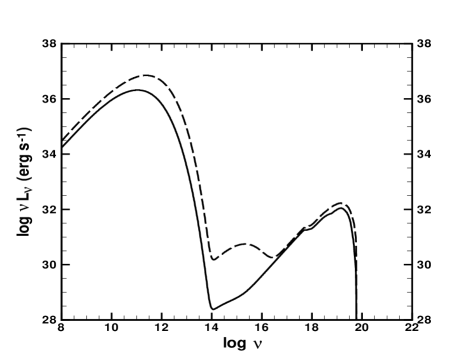
Fig. 13 shows the energy spectra calculated from model F with erg s-1 at s (dashed line) and with erg s-1 at s (solid line). The sub-milimetre and X-ray bumps in these spectra are originated from the synchrotron cooling by thermal electrons and the bremsstrahlung cooling, respectively, whose formulas are prescribed in Narayan & Yi (1995) and Stepney & Guilbert (1983). The intensities in the sub-milimetre bumps of models E and F are a little higher and the peak positions lie in a longer wavelength compared with the observational spectra at the quiescent state of Sgr A*. To the contrary, the intensities in the X-ray band (2–8 keV) are one orders of magnitude lower than the observed one. The radiatively inefficient accretion flow models (Yuan, Quataert & Narayan, 2003), such as the ADAFs, take into account the complicated physics including synchrotron and inverse Compton emission by thermal and non-thermal electrons under the two-temperature assumption and describe the energy spectra very fitted to the observed ones of Sgr A* over a wide range of energy bands from the radio to X-ray. In this respect, the present our model is too simple and insufficient to reproduce the spectra of Sgr A* but it is useful to examine the basic scenario of the low angular momentum flow model.
7 Summary and discussion
Based on the analysis of the angular momentum of the accretion flow around Sgr A* by Mościbrodzka, Das & Czerny (2006), we examined a low angular momentum flow model for Sgr A* using two-dimensional hydrodynamical calculations. The models with the specific angular momenta of 1.35, 1.55, 1.68, and 2.16 (in the usual nondimensional units) and input accretion rates of was considered. We summarize the results as follows.
(1) The accretion flow is very hot, optically thin, geometrically thick, and convectively unstable in the inner region of the accretion flow, as is also found in the ADAFs.
(2) The flow is highly advected and, if the syncrotron cooling and a two-temperature model are taken into account, the radiative efficiency of the accreting matter into radiation is very low, –, and the input accretion rate yr-1 results in the total luminosity which is comparable to the observed luminosity of Sgr A*.
(3) An irregularly oscillating shock is formed in the inner region of a few tens to a hundred and sixty Schwarzschild radii, except for the model with the highest . Due to the oscillating shock, the luminosity and the mass-outflow rate are modulated by several per cent to a factor of 5 and a factor of 2-7, respectively, on time-scales of an hour to ten days.
(4) The mass-outflow rate increases with increasing and it ranges over a few per cent, one-thirds, two-thirds and 99 per cent, of the input accreting matter, corresponding to the cases of = 1.35, 1.55, 1.68 and 2.16, respectively.
(5) The oscillaing shock is necessarily triggered if the specific angular momentum and the specific energy belong to or are located just nearby in the range of parameters responsible for a stationary shock in the rotating inviscid and adiabatic accretion flow.
(6) The time variability may be related to the flare phenomena of Sgr A*.
Since the specific angular momenta used in the models are reasonably estimated, the time variability of Sgr A* may be attributed naturally to the oscillating shock in the low angular momentum model considered here. Further evidence of the low angular momentum of the accretion flow around Sgr A* would confirm the validity of the models. If the specific angular mommentum of the accretion flow around Sgr A* is actually as small as , the time variability itself of the total emission like model F may explain the quiescent and the flare states of Sgr A*. On the other hand, in the case of higher angular momentum i.e. , the time modulation of the total emission is small to explain the flare phenomena of Sgr A*. However, under this circumstance , we expect that the large episodic wind caused by the non-stationary shock may induce the flare phenomena of Sgr A*. The flare phenomena of Sgr A* have been seen to be polarized in the radio, sub-millimetre and IR bands (Genzel et al., 2003; Meyer et al., 2006a, b; Trippe et al., 2007; Eckart et al., 2006). This is a strong evidence for a magnetic field around Sgr A*. The episodic wind in our model may be accelerated as a relativistic jet by some mechanism such as magnetic reconnection process in a current seet under the magnetic field away from the accretion flow (Yuan et al., 2009). The jet will collide with the ambient matter and excite the matter as a hot emitter, especially at times of the episodic wind. The emission from the hot matter may be observed as the flares in X-ray. Furthermore, the jet expands and cools in the far distant interstellar matter and results in the synchrotron emission due to the electrons in the magnetic field. This may be observed as the radio flares with a time lag from the X-ray flares. The existence of the magnetic field plays an important role in the accretion flow. However, the magnetic field was not taken into account simultaneously with the hydrodynamics in our models. Thus, the current low angular momentum flow model is simple and can not reproduce the observed spectra of Sgr A*, as is successfully fitted over a wide range of the wavelength by ADAFs. For a spectral fitting, we have to treat the physics of the synchrotron and inverse Compton emission by the thermal and non-thermal electrons under the two-temperature model. A further magneto-hydrodynamical examination of the flow with a low angular momentum model including the above physics should be pursued in the future.
References
- Bondi (1952) Bondi H., 1952, MNRAS, 112, 195
- Chakrabarti (1989) Chakrabarti S. K., 1989, ApJ, 347, 365
- Czerny & Mościbrodzka (2008) Czerny B., Mościbrodzka M., 2008, in Schoedel R., Eckart A., Pfalzner S., Ros E., eds, Journal of Physics: Conference Series, Proceedings of ‘The Universe Under the Microscope-Astrophysics at High Angular Resolution’, held 21–25 April 2008, in Bad Honnef, Germany, 2008, Vol. 131, p. 012001
- Do et al. (2009) Do T., Ghez A.M., Morris M.R., Yelda S., Meyer L., Lu J.R., Hornstein S.D., Matthews K., 2009, ApJ, 691, 1021
- Genzel et al. (2003) Genzel R., Schödel R., Ott T., Eckart A., Alexander T., Lacombe F., Rouan D., Aschenbach B., 2003, Nature, 425, 934
- Eckart et al. (2006) Eckart A., Schödel R., Meyer L., Trippe S., Ott T., Genzel R., 2006, A&A, 455, 1
- Eckart et al. (2008) Eckart A. et al., 2008, A&A, 492, 337
- Kley (1989) Kley W., 1989, A&A, 208, 98
- Levermore & Pomraning (1981) Levermore C.D., Pomraning G.C., 1981, ApJ, 248, 321
- Melia (1992) Melia F., 1992, ApJ, 387, L25
- Melia, Liu & Coker (2001) Melia F., Liu S., Coker R., 2001, ApJ, 553, 146
- Meyer et al. (2006a) Meyer L., Schödel R., Eckart A., Karas V., Dovčiak M., Duschl W.J., 2006a, A&A, 458, L25
- Meyer et al. (2006b) Meyer L., Eckart A., Schödel R., Duschl W.J., Mužić K., Dovčiak M., Karas, V., 2006b, A&A, 460, 15
- Meyer et al. (2008) Meyer L., Do T., Ghez A., Morris M.R., Witzel G., Eckart A., Bélanger G., Schödel R., 2008, ApJ, 688, L17
- Miyoshi et al. (2011) Miyoshi M., Shen Z.-Q., Oyama T., Takahashi R., Kato Y., 2011, PASJ, 63, 1093
- Molteni et al. (1996) Molteni D., Sponholz H., Chakrabarti S.K., 1996, ApJ, 457, 805
- Mościbrodzka, Das & Czerny (2006) Mościbrodzka M., Das T.K., Czerny B., 2006, MNRAS, 370, 219
- Nakayama (1994) Nakayama K., 1994, MNRAS, 270, 871
- Narayan & Yi (1994) Narayan R., Yi I., 1994, ApJ, 428, L13
- Narayan & Yi (1995) Narayan R., Yi I., 1995, ApJ, 452, 710
- Narayan & McClintock (2008) Narayan R., McClintock J.E., 2008, NewAR, 51, 733
- Okuda, Fujita & Sakashita (1997) Okuda T., Fujita M., Sakashita S., 1997, PASJ, 49, 679
- Okuda et al. (2004) Okuda T., Teresi V., Toscano E., Molteni D., 2004, PASJ, 56, 547
- Paczyńsky & Wiita (1980) Paczyńsky B., Wiita P.J., 1980, A&A, 88, 23
- Pringle & Rees (1972) Pringle J.E., Rees M.J., 1972, A&A, 21, 1
- Shakura & Sunyaev (1973) Shakura N.I., Sunyaev R.A., 1973, A&A, 24, 337
- Stepney & Guilbert (1983) Stepney S., Guilbert P.W., 1983, MNRAS, 204, 1269
- Trippe et al. (2007) Trippe S., Paumard T., Ott T., Gillessen S., Eisenhauer F., Martins F., Genzel, R., 2007, MNRAS, 375, 764
- Yuan (2011) Yuan F., 2011, in Morris M.R., Wang Q.D., Yuan F., eds, The galactic center: A Window to the Nuclear Environment of Disk Galaxies. Proceedings of a workshop held at Shanghai, China on October 19–23, 2009. Astron. Soc. Pac., San Francisco, 2011, p. 346
- Yuan et al. (2009) Yuan F., Lin J., Wu K., Ho L.C., 2009, MNRAS, 395, 2183
- Yuan, Quataert & Narayan (2003) Yuan F., Quataert E., Narayan R., 2003, ApJ, 598, 301
- Yuan, Quataert & Narayan (2004) Yuan F., Quataert E., Narayan R., 2004, ApJ, 606, 894
- Yusef-Zadeh et al. (2009) Yusef-Zadeh F. et al., 2009, ApJ, 706, 348
- Yusef-Zadeh et al. (2011) Yusef-Zadeh F., Wardle M., Miller-Jones J.C.A., Roberts D.A., Grosso N., Porquet D., 2011, ApJ, 729, 44