A derivation of (half) the dark matter distribution function

Abstract

All dark matter structures appear to follow a set of universalities, such as phase-space density or velocity anisotropy profiles, however, the origin of these universalities remains a mystery. Any equilibrated dark matter structure can be fully described by two functions, namely the radial and the tangential velocity distribution functions (VDF), and when we will understand these two then we will understand all the observed universalities. Here we demonstrate that if we know the radial VDF, then we can derive and understand the tangential VDF. This is based on simple dynamical arguments about properties of collisionless systems. We use a range of controlled numerical simulations to demonstrate the accuracy of this result. We therefore boil the question of the dark matter structural properties down to understanding the radial VDF.

1 Introduction

A growing number of seeming universalities have been identified in numerical simulations of dark matter structures. Most of these are integrated quantities, such as the density profile (Navarro et al., 1996; Moore et al., 1998), the pseudo phase-space density (Taylor & Navarro, 2001), and the velocity anisotropy (Hansen & Moore, 2006). The cause of these universalities remains, however, essentially unknown.

The origin of the universalities may lie in some fundamental property of dark matter, be it some statistical mechanics (Lynden-Bell, 1967; Hjorth & Williams, 2010) or optimization of some generalized entropy (Plastino & Plastino, 1993; Hansen et al., 2005; He & Kang, 2010; He, 2012). It may also be associated to dynamical effects, like radial orbit instability (Henriksen, 2009; Bellovary et al., 2008), or phase mixing or violent relaxation (Lynden-Bell, 1967; Kandrup et al., 2003). Alternatively, it could just be a “coincidence”, since all structures have been built up through similar processes of mergers and accretion (González-Casado et al., 2007; Salvador-Sole et al., 2007).

A first step towards answering the question of the origin of the integrated universalities, is to look at the actual distribution of velocities. Also the actual shape of the velocity distribution function (VDF) has been suggested to be universal (Hansen et al., 2006), which naturally could explain all the integrated universalities.

Asking the question about what dark matter structures fundamentally want, is different from asking what dark matter structures in an expanding universe actually end up doing. We will therefore not be considering structures from cosmological simulations, since their profiles often have merger history and environment dependent profiles. We will instead consider a range of numerical simulations where we have better control of their evolution. In this way we can repeatedly perturb the structures in controlled manners, as well as giving the structures sufficiently time that phase mixing between individual perturbations may be more complete than what is the case in cosmological simulations.

A non-trivial dark matter VDF also has direct implications for direct dark matter experiments (see e.g. Vergados et al. (2008); Fairbairn & Schwetz (2009); Kuhlen et al. (2010) for discussions and references).

We here present numerical evidence that the origin of the shape of the tangential VDF is simple dynamics, hence supporting the idea that dark matter wants to follow very simple dynamical rules. This explains the origin of the velocity anisotropy profile in the inner region of dark matter structures, with no seeming need for advanced statistical mechanical or generalized entropic principles. However, as we will point out, we are still left with an unknown origin of the radial VDF and hence also the density profile and the pseudo-phase space density profile are not explained yet.

Below we will explain the surprisingly simple dynamical reason for the full shape of tangential part of the VDF, and we will perform numerical simulations supporting this conclusion.

Some of these physical arguments have been presented previously (Hansen, 2009), however, the simulations presented here are significantly improved. In particular we create a set of controlled perturbations using energy exchange reminiscent of violent relaxation and dynamical friction, which allows the particle distributions to change significantly, without having the structure depart from spherical symmetry. At the same time the structures are analysed only after convergence to a fully stable configuration has been achieved.

2 Decomposition

Let us consider a particle moving in the smooth and spherical potential of many collisionless particles. The velocity of this particular particle can be decomposed into three components, namely the radial and the two tangential components. With such decomposition we can consider all particles in a given radial bin, and get the velocity distribution function (VDF) in both the radial and tangential directions. If the structure is non-rotating, then the two tangential VDF’s will be identical.

It has long been known that the radial and the tangential VDF’s are different, and physically this difference may seem very reasonable for equilibrated systems, as we will now explain.

We will first discuss the radial VDF. Consider a thin spherical bin, at radius $r$. If we consider the velocity components moving outwards in the radial direction, then those must be compensated by particles further out moving inwards. This compensation must depend on the particular density profile of the structure. This is most clearly seen in the Eddington inversion method (Eddington, 1916; Binney & Tremaine, 1987), from which one can easily derive the full radial VDF from the full density profile.

Now, let us instead consider the tangential velocity components. Instantaneously the components are moving in the tangential plane. For particles with the circular speed this means that the component is moving in constant density and constant potential. Particles moving slowly in the tangential plane will still be near the same density and potential after a short time interval. That implies that the equilibrium can be achieved simply by having other components in the same radial bin moving in the opposite direction. Therefore, whereas the radial VDF’s depend on the full radial density profile, then the tangential VDF’s apparently do not have to concern themselves with other radial bins. The tangential VDF could therefore, in principle, be the same at all radii.

This argument only holds instantaneously. Particles whose tangential velocity components are high, will after a longer time interval, $\Delta t$, be moving outwards into lower density regions, and will therefore later have converted their tangential component into both radial and tangential velocity components. Effectively this implies that the argument, that the tangential velocity component moves in constant potential and constant density, only holds for the low velocity particles. Below we will use numerical simulations to show that effectively the breakdown of this argument happens around $70\%$ of the escape velocity, $v_{\rm esc}$.

2.1 Low velocity component

We have argued above that the low velocity component of the tangential VDF should have a simple shape, which should be the shape of collisions-less particles moving in a constant potential and constant density. To simulate a uniform medium is rather difficult using N-body simulations, because any power or noise will induce gravitational collapse, which leads to a departure from homogeneity. Instead one can make a very simple analytical argument, which allows one to derive the VDF of a homogeneous medium.

Let us consider a spherical structure which has a known density profile, $\rho(r)$. If one has $\beta=0$, then we can use Eddington’s method to derive the VDF,

$$f(E)=\frac{1}{\sqrt{8}\pi^{2}}\int_{0}^{E}\frac{d^{2}\rho}{d\Psi^{2}}\frac{d\Psi}{\sqrt{E-\Psi}}\,,$$ (1)

where $\Psi(r)$ is the relative potential as a function of radius, and $E$ is the relative energy, $E=\Psi-mv^{2}/2$. Eddington’s method provides the unique ergodic distribution function (Binney & Tremaine, 1987). We use this method to find the VDF at all radii.

Imagine that the structure is particularly simple, namely with a constant density slope, $\gamma=d{\rm log}\rho/d{\rm log}r$, over a very large radial range. To be concrete, say that $\gamma=-2$ over 20 orders of magnitude in radius, and then truncated abruptly inside and outside this range. Eddington’s method shows us that this (isothermal sphere) has a VDF which is a Gaussian at all radii (except for the details arising from the truncation).

Now, consider a more shallow slope, e.g. $\gamma=-1.2$ or $-0.4$. For any value of $\gamma$ we can use Eddington’s method to calculate the VDF, and at any radius it will have exactly the same shape as function of $v_{r}/\sigma_{r}$. For each density slope we use this method to find the unique distribution function.

Finally we can extrapolate this approach to $\gamma=0$, which is identical to the case of constant density and constant potential. The shape of the VDF for this case is

$$f(v)\sim\left(1+\frac{v^{2}}{3\sigma^{2}}\right)^{-5/2}\,.$$ (2)

$\gamma=0$ is the condition for a particle moving in constant density and potential, and this is therefore the shape for the tangential VDF. In the case with $\gamma=0$ there is no difference between the radial and tangential directions, and the assumption of $\beta=0$ in the derivation is therefore correct, and the technique is thus self consistent.

We now have an analytical expression for the shape of the tangential VDF at small velocities, and only the normalizations are unknown. These are the overall normalization (which must be related to the density at that radius), and the normalization of the velocity (which is related to the tangential velocity dispersion).

2.2 High velocity component

The high velocity components are possibly even simpler to describe. If a velocity component is purely tangential at a given time, then shortly later it will be a combination of tangential and radial (unless it happens to have exactly the circular speed). We should therefore expect that the shape of the tangential and radial components are similar at high velocities.

There is only one complication, namely the normalization. The overall normalization must be identical between the radial and tangential components (since this is just the local density), however, as opposed to the low velocity component discussed above, the normalization of the high velocities components must be absolute, i.e. $v_{\rm rad}\sim v_{\rm tan}$.

2.3 The transition

The transition from the low to the high velocity components in a real system must be smooth, and is probably rather non-trivial, however, for simplicity we will here make the approximation that the transition is abrupt, and we make no attempt to make it smooth. Practically, we simply assume that the transition always happens near $0.7\,v_{\rm esc}$. We will address this issue further in the discussion section.

3 Simulations

The first simulation is a cold collapse, where the inclusion of substructure breaks the spherical symmetry. We distributed $5\times 10^{5}$ particles according to a Hernquist density profile (Hernquist, 1990) with scale radius $1$, and a cutoff at $200$. In addition $5\times 10^{5}$ particles, with the same mass as the main halo particles, were distributed in $24$ identical subhaloes, also having Hernquist density profiles, but with a scale radius of $0.5$ and a cutoff radius of $5$. The centers of the subhaloes were sampled in the same way as the particles in the main halo. The velocities of all the particles were initially zero. The total mass in the simulation was $1$. We ran the simulation for 200 time units, which corresponds to 200 dynamical times at the scale radius for the initial structure. Such a cold collapse is similar to the simulations by van Albada (1982).

For all the non-cosmological simulations discussed here, we used the parallel N-body simulation code, Gadget2 (Springel, 2005). For further details on the cold collapse see Sparre & Hansen (2012).

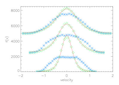
Figure 1: Radial (blue stars) and tangential (green diamonds) VDF for three radial bins in the cold collapse simulation. From top to bottom the radial bins are at $\gamma=-1.6,-2.0$ and $-2.4$, and the bins are shifted vertically to improve readability. The red (solid) lines are all of the same theoretical shape in eq. (2), which are seen to provide an acceptable fit in the low velocity region.

To sample the VDF’s we distribute the particles in radial bins with the same number of particles in each bin. In Figure 1 we show both the radial (blue stars) and tangential (green diamonds) VDF for three radial bins, chosen near a slope of $\gamma=-1.6,-2.0$ and $-2.4$ (from top to bottom). We also show the predicted shape of the tangential VDF (solid line), which is clearly seen to provide an acceptable fit in the low velocity region. It is also clear that the radial and the tangential VDF’s are very different in the low velocity region.

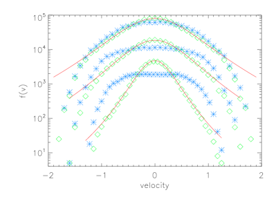
Figure 2: Same as figure 1, only linear-log to see details of the high-energy tail. Radial (blue stars) and tangential (green diamonds) VDF for three radial bins in the cold collapse simulation. From top to bottom the radial bins are at $\gamma=-1.6,-2.0$ and $-2.4$, and the bins are shifted vertically to improve readability. The red (solid) lines are of the theoretical shape for the low velocity region. For the high velocities it is clearly seen that the radial and the tangential VDF’s approach each other rapidly.

To see the details of how the radial and tangential VDF’s start agreeing in the high velocity region we plot the VDF’s from the same three radial bins in a lin-log space in Figure 2. It is clear that for high velocity particles the radial VDF’s (blue stars) are in good agreement with the tangential VDF’s (green diamonds). Interestingly, the tangential VDF’s can be approximated with the theoretical solid curve for low energies, and with the radial VDF’s for high velocities. And for the radially innermost bins (at slopes shallower than $-2$) this transition happens to be just around $v=0.7\,v_{\rm esc}$. Only for radial bins further out than $\gamma=-2$, it seems needed to use a more smooth transition.

3.1 G-perturbations

In order to test further the theoretical claims for the tangential VDF, we wish to construct a perturbation/equilibration scheme, which allows the VDF’s to change significantly, without having the structure depart from spherical symmetry.

We set up structures in perfect equilibrium. These structures may have any density profile, and have zero anisotropy or follow and Osipkov-Merritt beta profile (Binney & Tremaine, 1987). Now we increase the value of the gravitational constant by $20\%$. This increases the potential and makes the structure contract, and after a few dynamical times a new equilibrium is reached. Next we repeatedly increase or decrease the gravitational constant, and between each change we allow the structure to phase-mix and find a new equilibrium. After 20 such perturbations we use the standard value of $G$, and let the structure relax completely. For further details, see  Sparre & Hansen (2012).

In Figure 3 we show three radial bins from a simulation which initially was constructed as an isotropic Hernquist profile. This in particular means that the initial conditions (before the G-perturbations were executed) had identical radial and tangential VDF’s. Now, after the perturbations and subsequent relaxation there is a large difference between the radial and tangential VDF for small velocities. Instead, at high velocities the tangential and radial VDF quickly approach one another. As is also visible from the figure, the tangential VDF is well fitted by the theoretical prediction for small velocities.

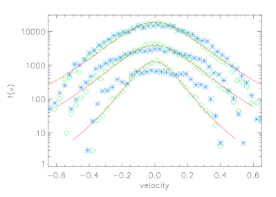
Figure 3: Radial and tangential VDF for three radial bins in the G-perturbation simulation. From top to bottom the radial bins are at $\gamma=-1.8,-2.3$ and $-3$, and the bins are shifted vertically to improve readability. All the red (solid) lines are of the same theoretical shape in eq. (2) for the low velocity region. For the high velocities it is clearly seen that the radial and the tangential VDF’s are very similar.

3.2 Explicit energy exchange

Collisionless particles experience different kinds of energy exchange between each other, in particular through violent relaxation (where the changing potential implies that the particle energies change), and through dynamical friction (which transfers energy from the fast to the slower particles). We therefore consider a perturbation where the spherical symmetry is again conserved, however, we allow the particles to exchange energy amongst each other. This is done in such a way, that each radial bin conserves energy, whereby both density and dispersion profiles are unaffected by the perturbation itself. This energy exchange is instantaneous and the subsequent evolution is with normal collisionless dynamics. After each perturbation we again allow for sufficient phase mixing (see Hansen, Juncher & Sparre, 2010, for details). After sufficiently many perturbations (typically 20 or 30) the structures have converged to a stable state, which will not change when exposed to further similar perturbations (Hansen, Juncher & Sparre, 2010; Barber et al., 2012).

In Figure 4 we present the VDF from three radial bins in the final structure, which are taken at density slopes of $\gamma=-1.7,-2.4$ and $-3.0$. Again we see that the final VDF’s agree well between the radial and tangential for high velocity components, and that the low velocity components are well fitted by the analytical expression.

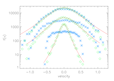
Figure 4: Radial and tangential VDF for three radial bins after perturbations by explicit energy exchange. From top to bottom the radial bins are at $\gamma=-1.7,-2.4$ and $-3.0$, and the bins are shifted vertically to improve readability. The red (solid) lines are of the theoretical shape for the low velocity region. For the high velocities it is clearly seen that the radial and the tangential VDF’s rapidly approach each other.

4 Discussions

We have demonstrated that three extremely different artificial and controlled perturbations all lead to a tangential VDF, which is in good agreement with the theoretical prediction. This result is in good agreement with earlier studies including head-on collisions and galaxy formation (Hansen et al., 2006; Hansen, 2009), and provides very strong evidence that the origin of the shape of the dark matter tangential VDF is indeed as simple as explained in section 2.1. An important difference from earlier studies is that we have here been investigating structures which have been exposed to controlled perturbations, and analysed only after convergence to a stable configuration has been achieved.

Let us remind the idea behind this paper. If we know the radial and the tangential VDF, then we know everything else, such as the phase-space density, the velocity anisotropy and the density profiles. For some idealized structures it is possible to derive the radial VDF directly from the density profile, and our results here imply that in that case we can derive the tangential VDF. That is, if we have the radial VDF, then we can derive the tangential VDF.

In the derivation of the tangential VDF we made no assumptions about the anisotropy of the system, and the tangential VDF should therefore be the same for all systems and at all radii, irrespective of their anisotropy profiles. This statement naturally only holds for realistic systems which have been perturbed and allowed to relax. One can always create systems in a quasi equilibrium states which may even have highly different distribution function. Systems created away from an equilibrium state most often also have very different tangential distribution functions. However, as we are demonstrating in this paper, all systems which are exposed to sufficient perturbations and subsequently allowed to relax to a quasi equilibrium state, will indeed have a tangential VDF of exactly this shape. In figure 5 we present the anisotropy profiles for the 3 systems considered. In particular one sees that the anisotropy has a strong radial variation, going from essentially isotropic in the central region, to radially dominated orbits in the outer regions. And yet the shape of the tangential VDF is the same at all radii.

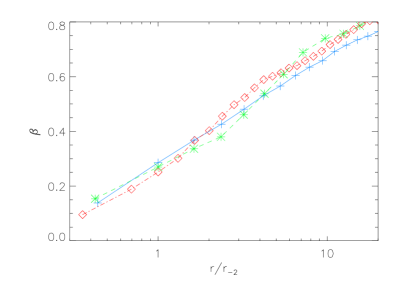
Figure 5: The radial variation of $\beta$ as function of radius for the structures considered in figures 1-4 (solid line HJS perturbation, dashed line G-perturbation, dot-dashed line infall simulation). The structures all have a strong variation, going from essentially isotropic towards the central region, to radial orbits in the outer regions.

It has previously been suggested that possibly the radial VDF is sufficiently close to a rescaled VDF resulting from the Eddington method (Hansen, 2009). We have tested this suggestion by fitting the density profile and then using the Eddington method to extract the radial VDF at all radii. However, the resulting VDF is not an accurate representation of the actual radial VDF. This means that we are still not at the point of understanding the radial VDF.

One interesting aspect of the arguments presented for the shape of the tangential VDF is, that for $\gamma=0$ it should be identical to the radial one. That trend is already clear from the figures, namely that the tangential VDF is suggestively close to the radial one for the innermost bins (upper curves in all figures). To test this further, we selected a radial bin in the inner region (outside of 5 times the softening length for each structure, and also outside a further 30.000 particles). The result is seen in Figure 6, where the tangential (dashed) and radial (solid) VDF’s are seen to be very similar. The local density slope at these bins were ranging from $\gamma=-0.4$ to $-1$ (bottom to top on Figure 6).

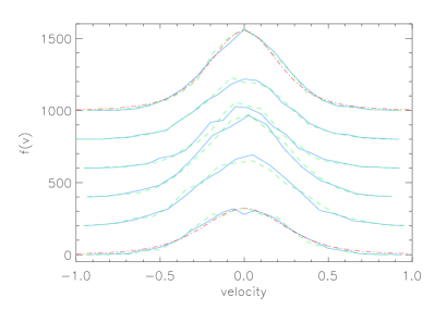
Figure 6: Radial (solid) and tangential (dashed) VDF for an inner bin (but not including approximately 35.000 of the most central particles). It is clear, that for all the structures the radial and tangential VDF are very similar. We add the same theoretical shape of eq. (2) in red (dot-dashed) lines, just to demonstrate the agreement. The structures included here are the cold collapse, two different G-perturbations and three different HJS2010 perturbations, covering a range of initial density and anisotropy profiles, in particular do we here present results for structures which were initially set up with a shallow central density profile. Velocities are scaled by the escape velocity and shifted vertically to improve readability. For this figure we selected structures which were created with zero inner slope, $\gamma_{\rm initial}=0$, before perturbations were applied.

We have discussed that the transition between high and low velocity may be approximated as a rather sharp transition. This is certainly a good approximation for the inner region (inside a slope of $\gamma=-2$). However, at larger radii it is clear, that a more smooth transition would provide a more accurate representation of the tangential VDF. For all the radial bins and for all the structures considered in this paper, we have estimated the best velocity for the transition, $v_{\rm trans}$, and it appears that this transition is in the range $0.6\,v_{\rm esc}<v_{\rm trans}<0.8\,v_{\rm esc}$. Thus, in order to avoid unnecessary fitting parameters, it is a rather good approximation to fix this at $v_{\rm trans}=0.7\,v_{\rm esc}$.

5 Conclusions

We have demonstrated that half of the distribution function (specifically, the tangential velocity distribution function) for dark matter structures can be understood from simple dynamical arguments. This implies that when we will eventually be able to derive the other half (namely the radial velocity distribution function), then we understand all the properties of dark matter structures, including the seeming universalities of the density, phase-space density and velocity anisotropy profiles.

We saw that the derivation of the tangential VDF did not require any reference to statistical mechanics or generalized entropy, but instead appears as a result of very simple dynamics. It now remains to derive the radial VDF, and it will be interesting to see if this will also be possible based on similar basic dynamical arguments.

Acknowledgements
The Dark Cosmology Centre is funded by the Danish National Research Foundation. The simulations were performed on the facilities provided by the Danish Center for Scientific Computing.

References

- Barber et al. (2012) Barber, J. et al. 2012, MNRAS (to appear) arXiv:1204.2764
- Bellovary et al. (2008) Bellovary, J. M., Dalcanton, J. J., Babul, A., et al. 2008, ApJ, 685, 739
- Binney & Tremaine (1987) Binney, J., & Tremaine, S. 1987, Princeton, NJ, Princeton University Press, 1987, 747 p.
- Eddington (1916) Eddington, A. S. 1916, MNRAS, 76, 572
- Fairbairn & Schwetz (2009) Fairbairn, M., & Schwetz, T. 2009, J. Cosmology Astropart. Phys, 1, 37
- González-Casado et al. (2007) González-Casado, G., Salvador-Solé, E., Manrique, A., & Hansen, S. H. 2007, arXiv:astro-ph/0702368
- Hansen (2009) Hansen, S. H. 2009, ApJ, 694, 1250
- Hansen et al. (2005) Hansen, S. H., Egli, D., Hollenstein, L., Salzmann, C. 2005, New Astron. 10, 379
- Hansen, Juncher & Sparre (2010) Hansen, S. H., Juncher, D., & Sparre, M. 2010, ApJ, 718, L68
- Hansen & Moore (2006) Hansen S. H., & Moore B 2006, New Astron., 11, 333
- Hansen et al. (2006) Hansen, S. H., Moore, B., Zemp, M., & Stadel, J. 2006, Journal of Cosmology and Astro-Particle Physics, 1, 14
- He (2012) He, P. 2012, MNRAS, 419, 1667
- He & Kang (2010) He, P., & Kang, D.-B. 2010, MNRAS, 406, 2678
- Henriksen (2009) Henriksen, R. N. 2009, ApJ, 690, 102
- Hernquist (1990) Hernquist, L. 1990, ApJ, 356, 359
- Hjorth & Williams (2010) Hjorth, J., & Williams, L. L. R. 2010, ApJ, 722, 851
- Kandrup et al. (2003) Kandrup, H. E., Vass, I. M., & Sideris, I. V. 2003, MNRAS, 341, 927
- Kuhlen et al. (2010) Kuhlen, M., Weiner, N., Diemand, J., et al. 2010, J. Cosmology Astropart. Phys, 2, 30
- Lynden-Bell (1967) Lynden-Bell, D. 1967, MNRAS, 136, 101
- Moore et al. (1998) Moore, B., Governato, F., Quinn, T., Stadel, J. & Lake G. 1998, ApJ, 499, 5
- Navarro et al. (1996) Navarro, J. F., Frenk, C. S., & White, S. D. M. 1996, ApJ, 462, 563
- Plastino & Plastino (1993) Plastino, A. R., & Plastino, A. 1993, Physics Letters A, 174, 384
- Salvador-Sole et al. (2007) Salvador-Solé, E., Manrique, A., González-Casado, G., & Hansen, S. H. 2007, ApJ, 666, 181
- Sparre & Hansen (2012) Sparre, M. & Hansen, S.H. 2012, subm to JCAP
- Springel (2005) Springel, V. 2005, MNRAS, 364, 1105
- Taylor & Navarro (2001) Taylor, J. E., & Navarro, J. F. 2001, ApJ, 563, 483
- Vergados et al. (2008) Vergados, J. D., Hansen, S. H., & Host, O. 2008, Phys. Rev. D, 77, 023509