Towards a Holographic Realization of Homes’ Law

Abstract:

Gauge/gravity duality has proved to be a very successful tool for describing strongly coupled systems in particle physics and heavy ion physics. The application of the gauge/gravity duality to quantum matter is a promising candidate to explain questions concerning non-zero temperature dynamics and transport coefficients. To a large extent, the success of applications of gauge/gravity duality to the quark-gluon plasma is founded on the derivation of a universal result, the famous ratio of shear viscosity and entropy density. As a base for applications to condensed matter physics, it is highly desirable to have a similar universal relation in this context as well. A candidate for such a universal law is given by Homes’ law: High $T_{c}$ superconductors, as well as some conventional superconductors, exhibit a universal scaling relation between the superfluid density at zero temperature and the conductivity at the critical temperature times the critical temperature itself. In this work we describe progress in employing the models of holographic superconductors to realize Homes’ law and to find a universal relation governing strongly correlated quantum matter. We calculate diffusive processes, including the backreaction of the gravitational matter fields on the geometry. We consider both holographic s-wave and p-wave superconductors. We show that a particular form of Homes’ law holds in the absence of backreaction. Moreover, we suggest further steps to be taken for holographically realizing Homes’ law more generally in the presence of backreaction.

*xcolor *color

1 Introduction

Gauge/gravity duality has proved to be a valuable tool for exploring strongly coupled regimes of field theories. The best studied example so far for applications to experimentally accessible strongly coupled systems is the application to the quark-gluon plasma. A very important example for this is the derivation of the famous result for the ratio of the shear viscosity and the entropy density [1],

$$\frac{\eta}{s}=\frac{1}{4\pi}\frac{\hbar}{k_{\text{B}}}.$$ (1)

Here the physical constants $\hbar$ and $k_{\text{B}}$ are written out explicitly in order to illustrate the influence of quantum mechanics and thermal physics. It has been shown [2, 3, 4] that this result applies universally for any isotropic gauge/gravity duality model based on an Einstein-Hilbert action on the gravity side. Exceptions are found by considering higher curvature corrections [5] or anisotropic configurations, see[6, 7] and [8]. Recently, the focus of applying the tools of the gauge/gravity duality has been widened to other strongly coupled systems in physics, especially to problems in condensed matter physics. In particular, significant progress has been made in describing holographic fermions (see [9, 10, 11] and references therein), superconductors/superfluids (for instance [12, 13, 14, 15, 16] and references therein) and to some extent also to lattices [17, 18]. For obtaining a solid general framework for condensed matter applications of the gauge/gravity duality, it would be very useful to derive a universal relation, similar in importance to (1), designed in particular for applications in condensed matter physics. Interestingly, the result (1) may be understood in the context of condensed matter physics by a time scale argument. Here, the properties of quantum critical regions [19, 20] give rise to a universal lower bound

$$\tau_{\hbar} =\frac{\hbar}{k_{\text{B}}T},$$ (2)

sometimes called “Planckian dissipation” [21] which can be compared to the possible lower bound for $$\nicefrac{{\eta}}{{s}}$$ given in (1). This seems to imply that the “strange metal phase” is a nearly perfect fluid without a quasi-particle description as is the quark-gluon plasma, since both cases do not allow for long-lived excitations compared to the energy

$$\frac{\hbar}{\tau} \ll\epsilon,$$ (3)

but rather describe a regime characterized by

$$\tau \sim\frac{\hbar}{\epsilon}.$$ (4)

In the case of the quark-gluon plasma, a possible characteristic time scale can be defined by

$$\eta \sim\epsilon\tau.$$ (5)

In typical condensed matter problems at quantum critical points, the relevant energy scale $\epsilon$ is set by the thermal energy $\epsilon\sim k_{\text{B}}T$. An interesting, yet unresolved problem, are the high temperature superconductors and their possible relation to quantum critical regions. A very interesting universality shown by almost all types of superconductors is Homes’ law. As explained in Section 2 in detail, this shows some connections to quantum critical regions and the “Planckian dissipation” time $\tau_{\hbar}$. Thus, it is an exciting candidate to find a universal relation for strongly coupled condensed matter systems [22] where the usual quasi-particle picture seems to fail.
In this paper, we outline how Homes’ law may be implemented in holography. We follow a simple approach which allows to demonstrate the validity of Homes’ law in the absence of backreaction of the matter fields on the geometry. We also find that our straightforward approach requires modifications in the presence of backreaction. We present and discuss possible generalizations and indicate directions for further research. The paper is organized as follows. In Section 2 we give a self-contained exposition of Homes’ law and discuss related condensed matter concepts and their holographic realization. In the Sections 3 and 4 we consider holographic s-wave and p-wave superconductors, respectively. In particular, we focus on the effects that arise from the backreaction of the gravitational interaction with the matter fields onto the geometry, governing the gravity dual. For this purpose, we numerically determine the phase diagram where we use the strength of the backreaction as parameter in addition to the ratio of temperature and chemical potential. This sets the ground for the calculations of various diffusion constants, which are discussed for the s-wave superconductor in Section 3.5 and for the p-wave superconductor in Section 4.3. We focus on the critical diffusion and associated time scales, i.e. the diffusion at the critical ratio of temperature and chemical potential depending on the backreaction at which the system transits to the superconducting phase. We find that a particular version of Homes’ law is satisfied if the backreaction is absent, while further work is required for the case with backreaction, as we explain. Finally, in Section 5 we summarize our results and give some possible explanations why Homes’ law is not confirmed in the approach considered here once the backreaction on the geometry is turned on. Some extensions of our original setup to remedy this are discussed in Section 6 along with some new perspectives on holographic superfluids/superconductors that might be of interest to pursue on their own.

2 Homes’ Law

With the discovery of high temperature superconductors, the new era heralded by the discovery of novel phases of (quantum) matter boosted the need for a new understanding of the classification of condensed matter systems. The experimental progress in controlling strongly correlated electronic systems and the exploration of strongly coupled fermionic/bosonic systems with the help of ultracold gases presented a new picture of nature that shook the old foundations of traditional condensed matter theory, i.e. Landau’s Fermi liquid theory and transitions between different phases classified by their symmetries. Famous examples departing from this old scheme are – apart form the high temperature superconductors – topological insulators, quantum critical regions connected to quantum critical points, and (fractional) quantum Hall effects, just to name a few (see [23, 24, 19, 20, 25] and references therein). As in particle physics, modern condensed matter theory is concerned with low-energy excitations that are described most efficiently by quantum field theories which reveal the universality of very different microscopic quantum many-body systems. However, in the strongly interacting cases, the “mapping” between the relevant degrees of freedom in the low-energy regime and the microscopic degrees of freedom are far from being clear and understood. Furthermore, it seems that quantum field theory alone is not enough to tackle strongly correlated systems and to explain these new states of (quantum) matter. Interestingly, the universality of Homes’ law seems to go beyond the artificial distinction between traditional and modern condensed matter physics since it displays a relation that works for conventional superconductors and high temperature superconductors which can be regarded as representatives of the old and the yet to be developed framework.

2.1 Homes’ Law in Condensed Matter

An interesting phenomenon to look for universal behavior in condensed matter systems, as advertised in the introduction to this section, is the universal scaling law for superconductors empirically found by Homes et al. [26] by collecting experimental results. This so-called Homes’ law describes a relation between different quantities of conventional and unconventional superconductors, i.e. the superfluid density $\rho_{\text{s}}$ at zero temperature and the conductivity $\sigma_{\text{DC}}$ times the critical temperature $T_{c}$,

$$\rho_{\text{s}}=C\sigma_{\text{DC}}(T_{c})T_{c},$$ (6)

where Homes et al. report two different values of the constant $C$ in units $\mathrm{[cm]^{-2}}$ for the different cases considered in [27]. The value $C=35$ is true for in-plane cuprates and elemental BCS superconductors, whereas for the cuprates along the c-axis and the dirty limit BCS superconductors they find $C=65$. The superfluid density $\rho_{\text{s}}$ is a measure for the number of particles contributing to the superfluid phase. It can be thought of as the square of the plasma frequency of the superconducting phase $\omega_{\text{Ps}}^{2}$, because the superconductor becomes “transparent” for electromagnetic waves with frequencies larger than

$$\rho_{\text{s}}\equiv\omega_{\text{Ps}}^{2}=\frac{4\pi n_{\text{s}}e^{2}}{m^{*}}.$$ (7)

Here $n_{\text{s}}$ denotes the superconducting charge carrier density which describes the number of superconducting charge carriers per volume (and is very different from the superfluid density $\rho_{\text{s}}$), $e$ is the elementary charge and $m^{*}$ is the effective mass of the charge carrier renormalized due to interactions. Another way to think about the superfluid density $\rho_{\text{s}}$ is the London penetration depth $\lambda_{\text{L}}$ which is basically the inverse of the superconducting plasma frequency, such that frequencies larger than $\omega_{\text{Ps}}$ correspond to length scales smaller than $\lambda_{\text{L}}$, i.e. $\rho_{\text{s}}\equiv\lambda_{\text{L}}^{-2}$. The critical temperature $T_{c}$ is determined by the onset of superconductivity. The conductivity $\sigma_{\text{DC}}$ and the superconducting plasma frequency $\omega_{\text{Ps}}$ are for instance obtained from reflectance measurements by extrapolation to the $\omega\to 0$ limit of the complex optical conductivity $\sigma(\omega)$,

$$\sigma_{\text{DC}} =\lim_{\omega\to 0}\operatorname{Re}\sigma(\omega), \omega_{\text{Ps}}^{2} =\lim_{\omega\to 0}\big{(}-\omega^{2}\operatorname{Re}\epsilon(\omega)\big{)},$$ (8)

since the high frequency limit of the real part of the dielectric function $\epsilon(\omega)$ is given by

$$\operatorname{Re}\epsilon(\omega)=\epsilon_{\infty}-\frac{\omega_{\text{Ps}}^{2}}{\omega^{2}}.$$ (9)

where $\epsilon_{\infty}$ is set by the screening due to interband transitions.

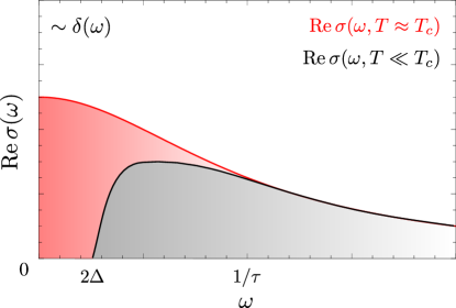
Figure 1: Schematic plots of the optical conductivity above the critical temperature $T_{c}$ and near the absolute zero $T=0$ for a dirty BCS superconductor. In the superconducting phase a gap develops for frequencies $\omega<2\Delta$. Note that in the dirty limit the quasi-particle scattering rate $\nicefrac{{1}}{{\tau}}$ is larger than $2\Delta$. The missing area (red shaded region) i.e. the difference between the area under the curve of $\operatorname{Re}\sigma(\omega,T\approx T_{c})$ and $\operatorname{Re}\sigma(\omega,T\ll T_{c})$ which condenses into the $\delta$-peak at $\omega=0$ and thus the superfluid strength (being the coefficient of the $\delta(\omega)$-function) is proportional to the missing area. Following the definitions given in (11) we see that the area under the $\operatorname{Re}\sigma(\omega,T\ll T_{c})$ curve determines $N_{\text{s}}$ whereas the red shaded area yields $N_{\text{n}}-N_{\text{s}}$.

Alternatively, the superconducting plasma frequency may be obtained from the optical conductivity measured above and below the critical temperature with the help of the oscillator strength sum rule

$$\frac{\omega_{\text{P}}^{2}}{8}=\int_{0}^{\infty}\operatorname{d\mathit{\omega}}\operatorname{Re}\sigma(\omega),$$ (10)

for the optical conductivity. This gives rise to an alternative definition of the superfluid density as compared to (8). We define the spectral weight in the normal and superconducting phase as follows,

$$N_{\text{n}} =\left.\int_{0}^{\infty}\operatorname{d\mathit{\omega}}\operatorname{Re}\sigma(\omega)\right|_{T>T_{c}}=\frac{\omega_{\text{Pn}}^{2}}{8}, N_{\text{s}} =\left.\int_{0^{+}}^{\infty}\operatorname{d\mathit{\omega}}\operatorname{Re}\sigma(\omega)\right|_{T<T_{c}}.$$ (11)

The superfluid density $\rho_{\text{s}}$ describes the degrees of freedom in the superconducting phase which have condensed into a Dirac $\delta$-peak at zero frequency, where $\rho_{\text{s}}$ can be viewed as the coefficient of $\delta(\omega)$. This $\delta$-peak in the real part of the conductivity gives rise to an infinite DC conductivity or zero resistivity. The superfluid density is equal to the difference between the integral over the optical conductivity (10) evaluated for $T<T_{c}$ and $T>T_{c}$ and generally yields identical values as compared to (8). Using the definitions of the spectral weight (11) we find

$$\rho_{\text{s}}=8\left(N_{\text{n}}-N_{\text{s}}\right).$$ (12)

This is the Ferrell-Glover-Tinkham sum rule. Note that in the definition of $N_{\text{s}}$ we have excluded the $\delta$-peak at $\omega=0$ because the oscillator strength sum rule (10) requires that the area under the optical conductivity curve is identical above and below $T_{c}$, i.e. in the superconducting and normal state. Thus (12) determines the missing area of the spectral weight that condensed into the $\delta$-peak at $\omega=0$, as illustrated in Figure 1. Although the gap describes the creation of Cooper pairs, it is really the missing area which gives rise to superconductivity, since according to (12) the missing area is equal to the degrees of freedom which condense at zero frequency, thus forming a new (coherent) macroscopic ground state with off-diagonal long range order. Semiconductors for instance are systems exhibiting an energy gap in their spectrum as well, but are not necessarily superconducting since there is no missing area and hence no new ground state let alone a phase transition. On the other hand, superconductors retain their properties even if the energy gap is removed (e.g. by magnetic impurities) due to the missing area under the $\operatorname{Re}\sigma(\omega)$ curve. As a caveat, let us note that high temperature superconductors may not satisfy the Ferrell-Glover-Tinkham sum rule, while it is expected to hold for dirty BCS superconductors.
In order to see clearly the relation between superfluid density and the product of the conductivity at the critical temperature and the critical temperature expressed by Homes’ law in (6), we have reproduced Table I from [27] with and without the elemental superconductors niobium Nb and lead Pb in Figure 2.

      

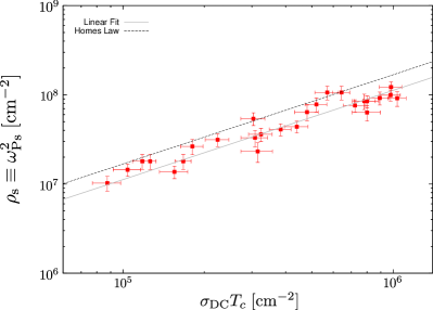
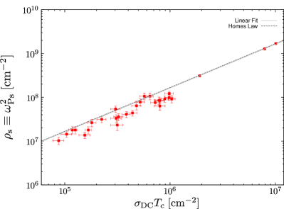
Figure 2: Plots of the complete data in Table 1 in [27]. The error bars are calculated by $\Delta(\omega_{\text{P}}^{2})=2\omega_{\text{P}}\Delta\omega_{\text{P}}$ and $\Delta(\sigma_{\text{DC}}T_{c})=T_{c}\Delta\sigma_{\text{D}C}$. The left plot shows data from high $T_{c}$ superconductors and for Ba_1-xK_xBiO3, while the one on the right includes three data points from elemental superconductors. As shown on the right the elemental conventional superconductors, two data points for Nb and one coming from the Pb superconductor, actually give Homes’ law as stated in [27]. If these three data points are ignored, as shown in the left panel, the linear fit is shifted and the data points are below the Homes’ law line.

Furthermore, in [26, 21, 27, 29] some possible explanations are given concerning the origin of Homes’ law: Conventional dirty-limit superconductors, marginal Fermi-liquid behavior, for cuprates a Josephson coupling along the c-axis or unitary-limit impurity scattering. Furthermore, the authors discuss limits where the relation breaks down, which is true in the overdoped region of cuprates. For dirty limit BCS superconductors, Homes’ law can be explained by the very broad Drude-peak which is condensing into the superconducting $\delta$-peak at $\omega=0$. The spectral weight of the condensate may then be estimated by an approximate rectangle of area $\rho_{\text{s}}\approx\sigma_{\text{DC}}\cdot 2\Delta$ in an optical conductivity plot, similar to Figure 1, where the gap in the energy of the superconducting state is denoted by $2\Delta$ and $\sigma_{\text{DC}}$ is the maximum of the curve at $\omega=0$. According to the BCS model, the energy gap in the superconducting phase is proportional to the critical temperature $T_{c}$ and thus $\rho_{\text{s}}\propto\sigma_{\text{DC}}T_{c}$. For high $T_{c}$ temperature superconductors the most striking argument can be found in [21] which links the universal behavior to the “Planckian dissipation” giving rise to a perfect fluid description of the “strange metal phase” with possible universal behavior, comparable to the viscosity of the quark-gluon plasma. The argument, reproduced here for completeness, relies on the fact that the right structure of $\rho_{\text{s}}$, $\sigma_{\text{DC}}$ and $T_{c}$ may be worked out by dimensional analysis: First, as already stated above (7) the superfluid density must be proportional to the density of the charge carriers in the superconducting state. The natural dimension for this quantity is $(\text{time})^{-2}$ so the product of $\sigma_{\text{DC}}$ and $T_{c}$ should have the same physical dimension. Second, the normal state possesses two relevant time scales, the normal state plasma frequency $\omega_{\text{Pn}}$ and the relaxation time scale $\tau$, which describes the dissipation of internal energy into entropy by inelastic scattering. One of the simplest combinations is the product of the two time scales which will yield the dimension $(\text{time})^{-1}$. Therefore we may take the optical conductivity to be of the Drude-Sommerfeld form (see Appendix B for details) given by

$$\sigma_{\text{D}C}=\frac{\omega_{\text{Pn}}^{2}\tau}{4\pi}=\frac{n_{\text{n}}e^{2}\tau}{m^{*}}.$$ (13)

The last and most crucial step is to convert the critical temperature into the dimension $(\text{time})^{-1}$. Energy and time are related by Heisenberg’s uncertainty principle and thus quantum physics and the idea of “Planckian dissipation” will enter,

$$\tau_{\hbar}(T_{c})^{-1} =\frac{k_{\text{B}}T_{c}}{\hbar}.$$ (14)

This time scale is the lowest possible dissipation time for a given temperature. For smaller time scales the system will only allow for quantum mechanical dissipationless motion. Interestingly, at finite temperature the lower bound can only be reached if the system is in a quantum critical state [19]. This implies that high $$T_{c}$$ superconductors exhibit a quantum critical region above the superconducting dome, which is supported by experimental evidence [30, 20]. To connect the expression on the right-hand-side of (6) with the left-hand-side, we can employ Tanner’s law [31] which states that

$$n_{\text{s}} \approx\frac{1}{4}n_{\text{n}}\,,$$ (15)

relating the superfluid density to the normal state plasma frequency, as can be seen from (7) and (13). This “explanation” of Homes’ law will guide us in order to find a holographic realization. We will expand on this idea in Section 2.2.

2.2 Homes’ Law in Holography

An obstacle towards checking Homes’ law directly within holography is that due to the conformal symmetry and the absence of a lattice, the Drude peak of the conductivity is given by a delta distribution even at finite temperatures above the critical temperature, i.e.

$$\operatorname{Re}\sigma(\omega) \sim\delta(\omega) \Leftrightarrow \qquad\operatorname{Im}\sigma(\omega) \sim\frac{1}{\omega}.$$ (16)

Thus, it is not possible to evaluate $\rho_{\text{s}}$ directly, which is related only to the superconducting degrees of freedom condensing at $\omega=0$. We therefore rewrite Homes’ law in such a way that it becomes accessible to simple models of holography. As we now discuss, this can be achieved by using the idea of Planckian dissipation following [21] for high temperature superconductors, as outlined above at the end of Section 2.1, or by employing the Ferrell-Glover-Tinkham sum rule (12) for dirty BCS superconductors as can be found in [29].
For simplicity, let us make two assumptions about holographic superconductors: First, let us assume that they satisfy the sum rule which requires that the area under the optical conductivity curve is identical in the superconducting phase and the normal phase. Second, we assume that all degrees of freedom condense in the superconducting state. Using the definition of the spectral weight in the normal phase $N_{\text{n}}$ (11) and the definition of the superconducting plasma frequency (7), we see that both plasma frequencies must be equal

$$\omega_{\text{Ps}}^{2} =\omega_{\text{Pn}}^{2},$$ (17)

which implies that $$N_{\text{s}}=0$$ in (12). Here we clearly neglect possible missing spectral weight as explained in the second paragraph of Section 2.1. In the holographic context, similar sum rules have been investigated in [32, 33, 34]. Alternatively, we may assume that the holographic superconductors obey Tanner’s law (18)

$$n_{\text{s}} =Bn_{\text{n}},$$ (18)

where $$n_{\text{s}} n_{\text{n}} B$$ and denotes the charge carrier density in the superconducting and the normal phase, respectively, and is a numerical constant. With either one of these two assumptions, we may rewrite Homes’ law in such a way that it becomes accessible to holography. Let us begin with the assumption that holographic superconductors fulfill the sum rule and that all degrees of freedom are participating in the superconducting phase: Starting from

$$\rho_{\text{s}}\equiv\omega_{\text{Ps}}^{2} =C\sigma_{\text{DC}}(T_{c})T_{c},$$ (19)

and assuming that the Drude-Sommerfeld model is still a useful approximation (see Appendix B for details) we can replace the conductivity by a characteristic time scale and the plasma frequency in the normal conducting phase

$$\sigma_{\text{D}C} =\frac{\omega_{\text{Pn}}^{2}\tau}{4\pi},$$ (20)

and thus (19) reads

$$\omega_{\text{Ps}}^{2} =C\frac{\omega_{\text{Pn}}^{2}}{4\pi}\tau_{c}T_{c},$$ (21)

where $$\tau_{c} \tau(T_{c})$$ denotes . (21) can be simplified using the assumption (17),

$$\tau_{c}T_{c} =\frac{4\pi}{C}.$$ (22)

(22) holds if there is no missing spectral weight and that all the spectral weight associated with the charge carriers condenses in the superconducting phase and hence contributes to the $$\delta$$-peak. This enables us to identify the plasma frequencies in the two different phases. Alternatively, we can use the assumption that the charge carrier densities in both states are proportional to each other. Starting again with

$$\rho_{\text{s}}\equiv 4\pi\frac{n_{\text{s}}e^{2}}{m^{*}} =C\sigma_{\text{DC}}(T_{c})T_{c},$$ (23)

and inserting the Drude-Sommerfeld optical conductivity in terms of the charge carrier density $$n_{\text{n}}$$

$$\sigma_{\text{D}C} =\frac{n_{\text{n}}e^{2}}{m^{*}}\tau,$$ (24)

we may write (23) as

$$n_{\text{s}} =\frac{C}{4\pi}n_{\text{n}}\tau_{c}T_{c}.$$ (25)

Assuming that the holographic superconductors obey (18) we arrive at

$$\tau_{c}T_{c} =\frac{4\pi B}{C}.$$ (26)

Note that the proportionality constants in (22) and in (26) may not coincide. If they do not, this will indicate that holographic superconductors behave either more like in–plane high temperature superconductors or like dirty-limit BCS superconductors. In any case the above simplifications allow us to circumvent the need to calculate spectral weights in the superconducting phase or the plasma frequency in either phase (some obstructions are discussed in Section 2.3), and to perform the calculation solely in the normal phase. Therefore we will extract the time scales in the normal phase of the s- and p-wave superconductors from diffusion constants, basically the momentum and R-charge diffusion denoted by $$D_{\text{M}} D_{\text{R}} D(T_{c})\propto\tau_{c}$$ and , respectively. In particular, since we obtain

$$D(T_{c})T_{c} =\text{const}.$$ (27)

This relation is directly accessible to holography. In fact, without including the backreaction of the gauge and matter fields on gravity, the diffusion constants are given by [1, 35, 36]

$$D_{\text{M}} =\frac{1}{4\pi T}, D_{\text{R}} =\frac{1}{4\pi T}\frac{d}{d-2},$$ (28)

such that

$$D_{\text{M}}T =\frac{1}{4\pi}=\text{const.}, D_{\text{R}}T =\frac{1}{4\pi}\frac{d}{d-2}=\text{const.},$$ (29)

where $d$ denotes the dimensionality of the spacetime, and thus Homes’ law is trivially satisfied in this case. This can be derived simply by dimensional analysis as is done in [37]. Extending the calculation of the diffusion constants to include backreaction we checked analytically and numerically that our results reduce to the known results in the limit where the backreaction vanishes. (see Sections 3.5 and 4.3 for details).

2.3 The Drude-Sommerfeld Model and Holography

The Drude-Sommerfeld model describes the properties of metals (i.a. electrical/thermal conductivities, heat capacities) by a simple model incorporating the behavior of the underlying charge carriers. The optical conductivity of the Drude-Sommerfeld model (13)

$$\sigma_{\text{D}C}=\frac{\omega_{\text{Pn}}^{2}\tau}{4\pi}=\frac{n_{\text{n}}e^{2}\tau}{m^{*}}.$$ (30)

possesses two scales, the plasma frequency $\omega_{\text{Pn}}^{2}$ setting the scale above which electromagnetic waves can enter the metal and the relaxation time scale $\tau$, connected to the mean free path $l=v_{\text{F}}\tau$ of the charge carriers (where the charge carrier density is denoted by $n$). Interactions between the charge carriers are included by the renormalization procedure generating effective masses $m^{*}$ and correction to the relaxation time. The inverse of the real part of the optical conductivity describes absorption processes/loss of energy which is related to dissipation, whereas the imaginary part describes dispersive processes/change of phase which is related to energy transport. The resistivity is defined as $(\operatorname{Re}\sigma(\omega=0))^{-1}$ and is the inverse of the maximum of the real part, the so called Drude peak. The width of the Drude peak is set by the relaxation rate $\tau^{-1}$. The imaginary part of (30) is a Lorentzian-shaped curve with maximal energy transport at resonance for $\omega=\tau^{-1}$. For very high frequencies $\omega>\omega_{\text{Pn}}$ the charge carriers are not able to follow the external excitation and thus the optical conductivity must approach zero.
Comparing our holographic setup to the above condensed matter discussion, we first notice that we do not have an underlying lattice. This implies that the Drude peak turns into a delta distribution (or $\delta$-peak) at $\omega=0$ since momentum conservation does not allow any dissipative process. In the large frequency limit, the optical conductivity approaches the non-vanishing conformal result, i.e. $\sigma(\omega\to\infty)=\text{const.}$, since the conformal symmetry does not permit any scale. In this sense there is no well-defined plasma frequency above which the system will become transparent, but a finite absorption due to the non-vanishing real part of the optical conductivity will be retained. A possible workaround is to define a regulated plasma frequency [32] which obey the Kramers-Kronig relations and thus the sum-rules. Moreover, we cannot compute effective masses $m^{*}$ or more generally, we cannot describe any physical parameter related to the lattice. Additionally, interesting physics is hidden in the zero frequency limit of the optical conductivity, which cannot be resolved without a lattice due to the $\delta$-peak arising from momentum conservation. One way to remedy these problems is to introduce a lattice explicitly as is done in different ways in [38, 17, 18, 39]. One of the results in [17] is the emergence of the Drude-Sommerfeld conductivity (102) in the low-frequency limit and – even more excitingly – in the mid-frequency range they find scaling behavior similar to cuprate superconductors. The use of an explicit lattice may be avoided by using the simplified form of Homes’ law stated in (22) or (26) which assumes either the validity of the sum rule or Tanner’s law, respectively. This fits in our overall scheme of looking at universal scaling behavior which should not be affected by an underlying microscopic lattice.

3 Holographic s-Wave Superconductor

In this section we give a self-contained exposition of the solution to the equations of motion derived from the Einstein-Maxwell action minimally coupled to a charged scalar field. For obtaining a family of holographic s-wave superconductors, we include the backreaction of the gauge field and the scalar field on the metric into our analysis. After explaining the normal phase solutions, i.e. solutions with a vanishing scalar field, we will employ a quasi-normal-mode analysis in order to determine the onset of the spontaneous condensation of the operator dual to the charged scalar field. For this purpose, we expand the action up to the quadratic order in the fluctuations about the background and derive the corresponding equations of motion. Finally, we determine the R-charge and momentum diffusion related to the gauge field fluctuations and the metric fluctuations, respectively. This allows us to calculate the function relevant for testing Homes’ law at finite backreaction.

3.1 Einstein-Maxwell Action

The best known (bottom up) holographic model to describe superconductivity is given by the Einstein-Maxwell action coupled to a charged scalar on the gravity side dual to a field theory with a conserved $U(1)$ current and an operator describing the condensate [40, 41, 13]. Rescaling the gauge field $A\to eA$ and the scalar field $\Phi\to e\Phi$ allows us to write the action in the form

$$S=\frac{1}{2\kappa^{2}}\int\operatorname{d^{\mathit{d+}1}\mathit{x}}\sqrt{-g}\left[R-2\Lambda-\frac{2\kappa^{2}}{e^{2}}\left(\frac{1}{4}F_{ab}F^{ab}-\left\lvert\nabla\Phi-\mathrm{i}A\Phi\right\rvert^{2}-V(\left\lvert\Phi\right\rvert)\right)\right],$$ (31)

where we have a dimensionless coupling parameter

$$\alpha^{2}L^{2}=\frac{\kappa^{2}}{e^{2}},$$ (32)

describing the strength of the backreaction onto the geometry exerted by the gauge field and the scalar field. On the field theory side, this parameter describes the ratio of charged degrees of freedom to the total degrees of freedom and thus can be considered as an effective chemical potential or in a loose sense some kind of “doping”. The equations of motions for the charged scalar field $\Phi$ derived from (31) are given by

$$\left(\nabla_{a}+\mathrm{i}A_{a}\right)\left(\nabla^{a}+\mathrm{i}A^{a}\right)\Phi^{\ast}-\frac{1}{2}V^{\prime}(\left\lvert\Phi\right\rvert)\frac{\Phi^{\ast}}{\left\lvert\Phi\right\rvert} =0,$$ (33)

$$\left(\nabla_{a}-\mathrm{i}A_{a}\right)\left(\nabla^{a}-\mathrm{i}A^{a}\right)\Phi-\frac{1}{2}V^{\prime}(\left\lvert\Phi\right\rvert)\frac{\Phi}{\left\lvert\Phi\right\rvert} =0.$$

Additionally, we have the Maxwell equations in curved spacetime

$$\nabla^{a}F_{ab}=j_{b},$$ (34)

which can be simplified to

$$\frac{1}{\sqrt{-g}}g_{ab}\partial_{c}\left(\sqrt{-g}F^{cb}\right)=\mathrm{i}\big{[}\Phi^{\ast}\left(\nabla_{b}-\mathrm{i}A_{b}\right)\Phi-\Phi\left(\nabla_{b}+\mathrm{i}A_{b}\right)\Phi^{\ast}\big{]}.$$ (35)

Finally, the Einstein equations sourced by the gauge field and by the scalar field are

$$R_{ab}-\frac{1}{2}Rg_{ab}+\Lambda g_{ab}=\alpha^{2}L^{2}\left(T_{ab}^{\text{em}}+T_{ab}^{\Phi}\right),$$ (36)

with

$$T_{ab}^{\text{em}} =g^{cd}F_{ac}F_{bd}-\frac{1}{4}g_{ab}F_{cd}F^{cd},$$ (37)

$$T_{ab}^{\Phi} =\left(\nabla_{a}\Phi^{\ast}+\mathrm{i}A_{a}\Phi^{\ast}\right)\left(\nabla_{b}\Phi-\mathrm{i}A_{b}\Phi\right)+\left(\nabla_{a}\Phi-\mathrm{i}A_{a}\Phi\right)\left(\nabla_{b}\Phi^{\ast}+\mathrm{i}A_{b}\Phi^{\ast}\right)$$

$$\hskip 12.0pt-g_{ab}\left(\nabla_{c}\Phi^{\ast}+\mathrm{i}A_{c}\Phi^{\ast}\right)\left(\nabla^{c}\Phi-\mathrm{i}A^{c}\Phi\right)-g_{ab}V(\left\lvert\Phi\right\rvert).$$ (38)

The most general planar and rotational symmetric solution to the set of equations (33)-(36) is the AdS-Reissner-Nordström black hole solution with scalar hair . Note that it is sufficient to assume that only quadratic terms are present in the potential $V(\left\lvert\Phi\right\rvert)=m^{2}\left\lvert\Phi\right\rvert^{2}$, since we are only interested in the behavior near the critical point where higher order interactions do not contribute.

3.2 Normal Phase Solutions of the Background Fields

As we are only interested in the phase diagram and since we are including the backreaction, it is advisable to simplify our discussion by considering the normal phase background solutions, i.e. $\Phi\equiv 0$, which reduces the equations of motion to

$$R_{ab}-\frac{1}{2}Rg_{ab}-\frac{d(d-1)}{2L^{2}}g_{ab} =\alpha^{2}L^{2}T_{ab}^{\text{em}},$$ (39)

$$g^{ab}\nabla_{a}F_{bc} =0.$$ (40)

The solutions to these equations are given by

$$\operatorname{d\mathit{s}}^{2}=\frac{L^{2}}{u^{2}}\left(-f(u)\operatorname{d\mathit{t}}^{2}+\operatorname{d\mathit{\mathbfit{x}}}^{2}+\frac{\operatorname{d\mathit{u}}^{2}}{f(u)}\right),$$ (41)

with

$$f(u) =1-\bar{M}\frac{u^{d}}{u_{\text{H}}^{d}}+\bar{Q}^{2}\frac{u^{2(d-1)}}{u_{\text{H}}^{2(d-1)}}, \bar{M} =1+\bar{Q}^{2}, \bar{Q} =\sqrt{\frac{d-2}{d-1}}\mu u_{\text{H}}\alpha,$$ (42)

where $\bar{M}$ and $\bar{Q}$ denotes the dimensionless mass and the dimensionless charge of the black hole, respectively. The gauge field solution including the constraints on the black hole horizon may be written as

$$A=\mu\left(1-\frac{u^{d-2}}{u_{\text{H}}^{d-2}}\right)\operatorname{d\mathit{t}},$$ (43)

where $\mu$ is the chemical potential, describing the difference in the electric potential between the horizon of the black hole at $u=u_{\text{H}}$ and the boundary of the AdS space (at $u=0$) and thus the energy of adding another charged particle to the black hole. Furthermore we may define a temperature related to the Bekenstein entropy by

$$T=\frac{1}{2\pi}\left[\frac{1}{\sqrt{g_{uu}}}\operatorname{\frac{d}{d\mathit{u}}}\sqrt{-g_{tt}}\right]_{u=u_{\text{H}}}=\frac{d-(d-2)\bar{Q}^{2}}{4\pi u_{\text{H}}}.$$ (44)

Since we are dealing with a scale invariant theory in the UV, the only dimensionless physical parameter is the ratio $\nicefrac{{T}}{{\mu}}$ which will be controlled (numerically) by the dimensionless chemical potential $\bar{\mu}=\mu u_{\text{H}}$. Using (42) we may write this ratio in terms of the charge of the black hole,

$$\frac{T}{\mu}=\frac{d-\frac{(d-2)^{2}}{d-1}\bar{\mu}^{2}\alpha^{2}}{4\pi\bar{\mu}}=\frac{d-(d-2)\bar{Q}^{2}}{\frac{4\pi}{\alpha}\sqrt{\frac{d-1}{d-2}}\bar{Q}},$$ (45)

and conversely

$$\bar{Q}_{\pm}=\frac{-2\pi\sqrt{d-1}\left(\frac{T}{\mu}\right)\pm\sqrt{4\pi^{2}(d-1)\left(\frac{T}{\mu}\right)^{2}+d(d-2)^{2}\alpha^{2}}}{\alpha(d-2)^{\frac{3}{2}}}.$$ (46)

In order to be consistent with the probe limit $\alpha\to 0$, we pick the positive solution of the quadratic equation for the black hole charge $\bar{Q}$, such that $\lim_{\alpha\to 0}\bar{Q}_{+}=0$.

3.3 Quasi-Normal-Mode Analysis and Phase Diagram

We use the holographic dissipation-fluctuation theorem [42] in order to determine the complex-valued Green’s function of scalar fluctuations about the fixed scalar background in the normal phase. Therefore we derive the quadratic action in the fluctuations

$$\phi(t,\mathbfit{x},u) =\Phi(u)+\delta\phi(t,\mathbfit{x},u),$$ (47)

$$A_{a}(t,\mathbfit{x},u) =A_{a}^{\text{B}}(u)+a_{a}(t,\mathbfit{x},u),$$

$$g_{ab}(t,\mathbfit{x},u) =G_{ab}(u)+h_{ab}(t,\mathbfit{x},u).$$

The detailed calculations and solutions are shown in Appendix C. For convenience we state the equation of motion for the scalar field fluctuations (107),

$$\delta\phi^{\prime\prime}(u)+\left(\frac{f^{\prime}(u)}{f(u)}-\frac{d-1}{u}\right)\delta\phi^{\prime}(u)+\left[\frac{(\omega+A_{t})^{2}}{f(u)^{2}}-\frac{\mathbfit{k}^{2}}{f(u)}-\frac{L^{2}m^{2}}{u^{2}f(u)}\right]\delta\phi(u)=0,$$ (48)

which we will use in order to determine the phase diagram. We are interested in the spontaneous symmetry breaking induced by the condensation of the operator dual to the scalar field $\Phi$. For a second order phase transition we can use the dissipation-fluctuation theorem to look for instabilities in the fluctuations. Thus, for a given fixed value of the backreaction $\alpha$, we vary the dimensionless parameter $\nicefrac{{T}}{{\mu}}$ and look for a quasi-normal mode crossing the origin of the complex frequency plane. Numerically, we solve (48) with infalling boundary conditions at the black hole horizon and calculate the corresponding retarded Green’s function for $\mathbfit{k}=\mathbfit{0}$ and $\omega=0$. We expect to find a gapless mode which is related to a pole in the retarded Green’s function, such that we may determine the set of parameters $(\alpha,\nicefrac{{T}}{{\mu}})$ yielding critical curves as shown in Figure 3.

      

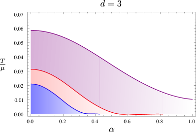
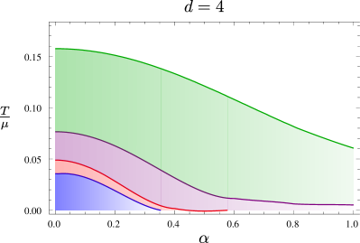
Figure 3: Phase diagram of the holographic s-wave superconductor for $d=4$ and $d=3$ as a function of the backreaction parameter $\alpha$, depending on the scalar field mass. Colored regions (for $d=3$ are encoded as $\color[rgb]{0,0,1}m^{2}L^{2}=4$, $\color[rgb]{1,0,0}m^{2}L^{2}=0$, $\color[rgb]{0.5,0,0.5}m^{2}L^{2}=-2$ and for $d=4$ we have $\color[rgb]{0,0,1}m^{2}L^{2}=5$, $\color[rgb]{1,0,0}m^{2}L^{2}=0$, $\color[rgb]{0.5,0,0.5}m^{2}L^{2}=-3$, $\color[rgb]{0,0.66796875,0}m^{2}L^{2}=-4$) show phases where the scalar field condenses yielding a superfluid phase.

Additionally, we can also vary the mass of the scalar field related to the scaling dimension of the dual operator via

$$\Delta_{\pm} =\frac{1}{2}\left(d\pm\sqrt{d^{2}+4L^{2}m^{2}}\right), \qquad\qquad m^{2}L^{2} =\Delta_{\pm}\left(\Delta_{\pm}-d\right).$$ (49)

The critical value of the backreaction for $T=0$ can be determined analytically by looking at the IR behavior near the black hole horizon. The corresponding charge of the black hole is given by

$$\bar{Q}^{2}=\frac{d}{d-2}.$$ (50)

Inserting this value into the metric (41), we find a double zero giving rise to an $\text{AdS}_{2}\times\mathds{R}^{d-1}$ metric and thus an IR fixed point

$$\operatorname{d\mathit{s}}^{2}_{\text{AdS}_{2}}=L^{2}\left(\varrho^{2}\operatorname{d\mathit{\tilde{t}}}+\frac{\operatorname{d\mathit{\varrho}}^{2}}{\varrho^{2}}\right),$$ (51)

with $\varrho=(u-u_{\text{H}})$ and rescaled $t$ and $\mathbfit{x}$ coordinates, accordingly. The $\text{AdS}_{2}$ radius is related to the $\text{AdS}_{d+1}$ radius by

$$L_{\text{AdS}_{2}}^{2}=\frac{L^{2}}{d(d-1)}.$$ (52)

The near horizon expansion of the background gauge field reads

$$A_{t}^{2}\approx\frac{d(d-1)}{u_{\text{H}}^{4}\alpha^{2}}(u-u_{\text{H}})^{2}=\frac{d(d-1)}{u_{\text{H}}^{4}\alpha^{2}}\varrho^{2}.$$ (53)

Finally, (48) can be written as

$$\delta\psi^{\prime\prime}(\varrho)+\frac{2}{\varrho}\delta\psi^{\prime}(\varrho)-\frac{L^{2}_{\text{AdS}_{2}}m^{2}}{\varrho^{2}}\delta\psi(\varrho)=0,$$ (54)

and the effective mass term can be compared to the Breitenlohner-Freedman stability bound for $\text{AdS}_{2}$,

$$L^{2}_{\text{AdS}_{2}}m^{2}_{\text{eff}}=\frac{1}{d(d-1)}\left(L^{2}m^{2}-\frac{1}{\alpha^{2}}\right)\leq L^{2}_{\text{AdS}_{2}}m^{2}_{\text{BF}}=-\frac{1}{4}.$$ (55)

This leads to a condition on $\alpha$ for scalar field condensation to occur,

$$\alpha^{2}\leq\frac{1}{\frac{d(d-1)}{4}+L^{2}m^{2}}.$$ (56)

We see if the mass is already below the $\text{AdS}_{2}$ Breitenlohner-Freedman bound, there is no critical value for $\alpha$ and hence no quantum critical point or phase transition at zero temperature between the condensed phase and the normal phase. The different masses used in the numerical calculation and the corresponding values for the scaling and the critical backreaction strength are listed in Table 1.

	$d=3$			$d=4$
$m^{2}L^{2}$	$4$	$0$	$-2$	$5$	$0$	$-3$	$-4$
$\Delta_{-}$	$-1$	$0$	$1$	$-1$	$0$	$1$	$2$
$\Delta_{+}$	$4$	$3$	$2$	$5$	$4$	$3$	$2$
$\alpha^{2}_{c}$	$\dfrac{2}{11}$	$\dfrac{2}{3}$	$-2$	$\dfrac{1}{8}$	$\dfrac{1}{3}$	$\infty$	$-1$

Table 1: List of the critical value for the strength of the backreaction $\alpha$ for different masses in three and four dimensions. Note that the instability condition is satisfied for $\alpha<\alpha_{c}$. In particular for the negative values we do not have a critical value of $\alpha\in\mathds{R}$, so in this case for $T=0$ we always find a condensed/superfluid phase.

Our results as displayed in Figure 3 show that the critical temperature decreases with increasing backreaction strength $\alpha$. Moreover, if the scalar mass is larger than a critical value, the critical temperature goes to zero for a finite value of $\alpha$. This is the case most reminiscent of a real high $T_{c}$ superconductor, when the dome in Figure 3 has similarities with the right hand side of the dome in the phase diagram of a high $T_{c}$ superconductor.
The physical interpretation of $\alpha$ is that it corresponds to the ratio of the number of $SU(2)$ charged degrees of freedom over all degrees of freedom [43]. The phase diagrams above indicate that an increase of $\alpha$ reduces the numbers of degrees of freedom which can participate in pair formation and condensation, such that $T_{c}$ is lowered. A similar mechanism also seems to be at work when adding a double trace deformation to the holographic superconductor [44], and has been discussed within condensed matter physics using a BCS approach in [45]. For holographic superconductors, this mechanism is most clearly visible for the top-down holographic superconductors involving D7 brane probes [46, 47] in which the dual field theory Lagrangian and thus the field content of the condensing operator are known. In these models, there is an $U(2)$ symmetry which factorizes into an $SU(2)_{I}\times U(1)_{B}$, i.e. into an isospin and a baryonic symmetry. A chemical potential is switched on for the $SU(2)_{I}$ isospin symmetry and the condensate is of $\rho$-meson form,

$$J_{x}{}^{1}=\bar{\psi}\sigma^{1}\gamma_{x}\psi+\bar{\phi}\sigma^{1}\partial_{x}\phi=\bar{\psi}_{\uparrow}\gamma_{x}\psi_{\downarrow}+\bar{\psi}_{\downarrow}\gamma_{x}\psi_{\uparrow}+\text{bosons},$$ (57)

where $\psi=(\psi_{\uparrow},\psi_{\downarrow})$ and $\phi=(\phi_{\uparrow},\phi_{\downarrow})$ are the quark and squark doublets, respectively, which involve up and down flavors, with $\sigma^{i}$ the Pauli matrices in isospin space and $\gamma_{\mu}$ the Dirac matrices. As an additional control parameter, a chemical potential $\mu_{B}$ for the baryonic $U(1)_{B}$ symmetry may be turned on. This leads to a decrease of $T_{c}$ [48] (see also [49]) which may be understood as follows: Under the $U(1)_{B}$ symmetry, $\psi$ and ${\bar{\psi}}$ have opposite charge. The same applies to $\phi$ and $\bar{\phi}$. Turning on $\mu_{B}$ leads to an excess of $\psi$ over $\bar{\psi}$ degrees of freedom, which implies that less degrees of freedom are available to form the pairs (57). The same applies to $\phi$ and $\bar{\phi}$ degrees of freedom. Thus in this case, charge carriers in the normal state are also present in the superconducting phase, leading to the formation of a pseudo-gap.

3.4 Diffusion Constants

As explained in Section 2, an analysis of Homes’ law requires the definition of a relevant time scale. Possible candidates for time scales are associated with diffusive processes. We may determine two different types of diffusion, momentum diffusion $D_{\text{M}}$ and R-charge diffusion $D_{\text{R}}$, respectively. The former can be related to the shear viscosity by studying hydrodynamic modes,

$$D_{\text{M}}=\frac{\eta}{\varepsilon+P},$$ (58)

such that it can be solely described by thermodynamic quantities using the famous result (1). The latter, however, cannot be calculated solely by thermodynamic quantities in general, such that an independent calculation for each background is necessary. Usually the charge diffusion constant can be read off from the dispersion relation $\omega=-\mathrm{i}D\mathbfit{k}^{2}$ of the conserved current, which can be derived from Fick’s law and the continuity equation

$$\mathbfit{j} =-D\nabla\rho, \qquad\dot{\rho}+\nabla\bm{\cdot}\mathbfit{j} =0, \longrightarrow \qquad\quad\dot{\rho}-D\nabla^{2}\rho =0.$$ and (59)

Fortunately, this work has already been done by [35] without backreaction.

Momentum Diffusion with Backreaction

Since we are working with a fixed chemical potential, we take the grand canonical ensemble to describe the momentum diffusion in the thermodynamic limit. Using the gauge/gravity duality the grand canonical potential is given by

$$\Omega=\frac{1}{\beta}I=TI,$$ (60)

where $I$ denotes the regularized Euclidean on-shell action given by

$$I=-\frac{L^{d-1}}{2\kappa^{2}}\frac{V_{d-1}}{T}\frac{1}{u_{\text{H}}^{d}}\left(1+\bar{Q}^{2}\right).$$ (61)

Using the Gauge/Gravity dictionary, we derive the charge density, the energy density and the entropy density from (60), with the help of the relations

$$s =\frac{4\pi}{2\kappa^{2}}\frac{L^{d-1}}{u_{\text{H}}^{d-1}},$$ (62)

$$\varepsilon =\frac{d-1}{2\kappa^{2}L^{d-1}}\frac{1+\bar{Q}^{2}}{u_{\text{H}}^{d}},$$

$$n =\sqrt{(d-1)(d-2)}\frac{L^{d-1}}{\kappa^{2}}\frac{\alpha\bar{Q}}{u_{\text{H}}^{d-1}}.$$

The black hole horizon $u_{\text{H}}$ should be understood as a function of $\mu$ or $T$, respectively, defined by solving either (42) or (44) for $u_{\text{H}}$, whereas $\bar{Q}$ is a function of $\nicefrac{{T}}{{\mu}}$ defined by the inversion of (46). Starting from the definition of the momentum diffusion and using the relations (1) and the first law of thermodynamics $\varepsilon=Ts-P+\mu n$, we find

$$D_{\text{M}}=\frac{\eta}{\varepsilon+P}=\frac{\frac{s}{4\pi}}{Ts+\mu n}=\frac{1}{4\pi T}\frac{1}{1+\frac{\mu}{T}\frac{n}{s}}.$$ (63)

Inserting the relations (45) for $\nicefrac{{\mu}}{{T}}$ and (62) for $\nicefrac{{n}}{{s}}$ we finally arrive at

$$D_{\text{M}}=\frac{1}{4\pi T}\left(1+\frac{2(d-1)\bar{Q}^{2}}{d-(d-2)\bar{Q}^{2}}\right)^{-1}.$$ (64)

R-Charge Diffusion with Backreaction

As explained in the previous subsection it is not straightforward to generalize the R-charge diffusion with backreaction to arbitrary dimensions. To our knowledge the functional dependence on the backreaction of $D_{\text{R}}$ in $d=3$ dimensions is not known yet, let alone for arbitrary dimensions $d$. Surely, this would be an interesting result which is beyond the scope of this work. In $d=4$ the R-charge diffusion with backreaction is determined in [50]. Converting the expression for $D_{\text{R}}$ into the form given by our conventions we find

$$D_{\text{R}}=\frac{1}{4\pi T}\frac{(2-\bar{Q}^{2})(2+\bar{Q}^{2})}{2(1+\bar{Q}^{2})}\,,$$ (65)

where the dimensionless black hole charge is defined in (42). Furthermore, we may look at the ratio of the two different diffusion constants,

$$\frac{D_{\text{R}}}{D_{\text{M}}}=2+\bar{Q}^{2}.$$ (66)

3.5 Discussion

Diffusion without backreaction for arbitrary $d$

      

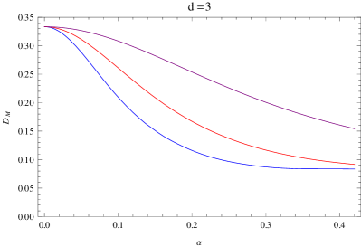
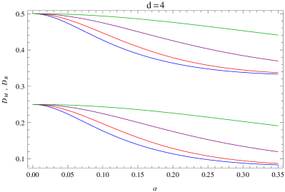
Figure 4: Plots of momentum diffusion constant $D_{\text{M}}$ for $d=3$ (left panel) and R-charge diffusion $D_{\text{R}}$ and momentum diffusion $D_{\text{M}}$ for $d=4$ (right panel) versus the backreaction strength $\alpha$. The color coding of the different scalar field masses follows Figure 3. The probe limit properties for $\alpha=0$ are reproduced, i.e. for $d=3$ we find $D_{\text{M}}=\nicefrac{{1}}{{3}}$ and in the case of $d=4$ $D_{\text{M}}=\nicefrac{{1}}{{4}}$ and $D_{\text{R}}=\nicefrac{{1}}{{2}}$, independently of the scalar field mass.

First of all we check our results by taking the limit of vanishing backreaction, i.e. setting $\alpha$ and $\bar{Q}$ to zero in (64) and (65). We see that the dimensionless temperature $\bar{T}$ (44) has the fixed value of $\nicefrac{{d}}{{4\pi}}$ and thus

$$\bar{D}_{\text{M}}=\frac{1}{4\pi\bar{T}}=\frac{1}{d},$$ (67)

is equal for all masses of the scalar field. Similarly, the R-charge diffusion is given by [37]

$$\bar{D}_{\text{R}}=\frac{1}{4\pi\bar{T}}\frac{d}{d-2}=\frac{1}{d-2},$$ (68)

and the ratio is given by

$$\frac{D_{\text{R}}}{D_{\text{M}}}=\frac{d}{d-2}.$$ (69)

Comparing these results to our numerical solutions shown in Figure 4, we see that for $\alpha=0$, we obtain for $d=3$ dimensions a dimensionless value of $\nicefrac{{1}}{{3}}$ for $D_{\text{M}}$. This is consistent with the values obtained form the analytic calculation without backreaction (67). In particular, we see that the momentum diffusion does not depend on the mass of the background scalar field since all diffusion constants for different masses (indicated in the figure by different colors) converge to the same value. Similarly for $d=4$, we check our numerical values for the momentum and the R-charge diffusion by comparing to the results without backreaction. As is displayed in Figure 4, we find that $D_{\text{M}}=\nicefrac{{1}}{{4}}$ and $\bar{D}_{\text{R}}=\nicefrac{{1}}{{2}}$ as stated in (67) and (68), as well as the correct value of the ratio $\nicefrac{{D_{\text{R}}}}{{D_{\text{M}}}}=2$. Again our numerical results are consistent with the analytic solutions without backreaction and we see the same convergence effect for the different masses of the scalar field for each diffusion constant displaying the independence on the scalar fields’ mass.

Momentum Diffusion for $d=3$

Inserting the critical values for $\nicefrac{{T}}{{\mu}}$ at a fixed $\alpha$, we may check how much the momentum diffusion is varying with respect to $\alpha$. As shown in Figure 5, there is a mild variation of the momentum diffusion in the sense that we are approaching the values for $\alpha=0$ in a linear way.

      

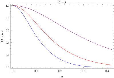
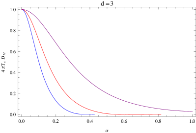
Figure 5: The constant $C_{\text{M}}$ related to momentum diffusion $D_{\text{M}}$ for $d=3$ and different masses of the scalar field (color coded as $\color[rgb]{0,0,1}m^{2}L^{2}=4$, $\color[rgb]{1,0,0}m^{2}L^{2}=0$ and $\color[rgb]{0.5,0,0.5}m^{2}L^{2}=-2$) plotted depending on the strength of the backreaction $\alpha$, defined in (32). The left panel shows the numerical values found by a minimization algorithm up to the $\alpha$ where poles of higher excitations in the Green’s function overlays with the lowest modes, thus leading to a breakdown of the algorithm. Only in the case of $\color[rgb]{0,0,1}m^{2}L^{2}=-2$, we have tested our algorithm up to $\alpha=1$. In the right panel we included the analytically determined critical points $\alpha_{c}$ for $\color[rgb]{0,0,1}m^{2}L^{2}=4$ and $\color[rgb]{1,0,0}m^{2}L^{2}=0$ given in Table 1 which corresponds to the zero temperature case with $\bar{Q}^{2}=\nicefrac{{d}}{{(d-2)}}$ and thus $C_{\text{M}}=0$. Due to the reduced number of data points we use an interpolation function in the region $\alpha\in[0.35,\sqrt{\nicefrac{{2}}{{3}}}\approx 0.82]$. For this reason the curves for $\color[rgb]{0,0,1}m^{2}L^{2}=4$ and $\color[rgb]{1,0,0}m^{2}L^{2}=0$ should not be trusted to be very accurate. Since for $\color[rgb]{0.5,0,0.5}m^{2}L^{2}=-2$ there is no critical value of $\alpha$, so $C_{\text{M}}$ approaches zero asymptotically.

In order to compare our numerical results to the constant governing Homes’ law rewritten in the form (22) or (26), we introduce the function

$$C_{\text{M}}=4\pi T_{c}D_{\text{M}}(T_{c})=\left(1+\frac{4\bar{Q}^{2}}{3-\bar{Q}^{2}}\right)^{-1},$$ (70)

plotted in Figure 5. Here we assume that the diffusive process is proportional to a time scale $\tau_{c}\propto D_{\text{M}}(T_{c})$, such that the proportionality does not depend on $\bar{Q}$ or $\alpha$.

R-Charge Diffusion and Momentum Diffusion for $d=4$

We now repeat the discussion of the previous subsection for the four-dimensional case. In addition to the momentum diffusion, we may also calculate the R-charge diffusion which will give us an additional time scale to choose.

      

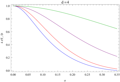
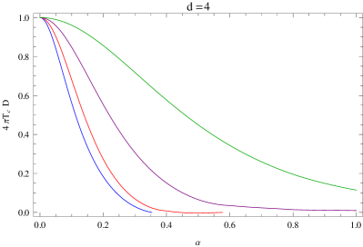
Figure 6: For $d=4$ dimensions: Dimensionless momentum diffusion given by $C_{\text{M}}$ depending on the backreaction $\alpha$ (for different masses of the scalar field color coded as $\color[rgb]{0,0,1}m^{2}L^{2}=5$, $\color[rgb]{1,0,0}m^{2}L^{2}=0$, $\color[rgb]{0.5,0,0.5}m^{2}L^{2}=-3$ and $\color[rgb]{0,0.66796875,0}m^{2}L^{2}=-4$). As already explained in Figure 5, the endpoint in the curves for scalar field mass $\color[rgb]{0,0,1}m^{2}L^{2}=5$ and $\color[rgb]{1,0,0}m^{2}L^{2}=0$ as shown in the right panel is set by the critical values of $\alpha$ listed in Table 1. Due to the interpolation these curves should be taken with a grain of salt in the vicinity of the critical point $\alpha_{c}$.

The constant related to $4\pi\tau_{c}T_{c}$ for the R-charge diffusion reads

$$C_{\text{R}} =\frac{(2-\bar{Q}^{2})(2+\bar{Q}^{2})}{2(1+\bar{Q}^{2})}.$$ (71)

Note that this function is running from $$2 0 \alpha\in[0,\alpha_{c}] \nicefrac{{1}}{{(2\pi T)}} d=4$$ to for since the R-charge diffusion without backreaction is given by see (68). For , the constant for the momentum diffusion reads

$$C_{\text{M}} =\left(1+\frac{3\bar{Q}^{2}}{2-\bar{Q}^{2}}\right)^{-1}.$$ (72)

Note also that the ratio $\nicefrac{{C_{\text{R}}}}{{C_{\text{M}}}}$ is given by $2$ in compliance with the ratio for the diffusion constants (69). The plots of $C_{\text{M}}$ and $C_{\text{R}}$ are shown in Figure 6 and Figure 7, respectively.

      

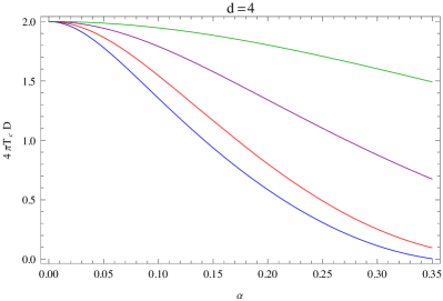
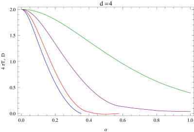
Figure 7: Dimensionless R-charge diffusion given by $C_{\text{R}}=4\pi T_{c}D_{\text{R}}$. Note that we have used the same prefactor in the definition (71) as for the dimensionless momentum $C_{\text{M}}$, which leads to the probe limit value of two. The color coding of the scalar field masses is identical to Figure 6.

We see that the numerically solutions are virtually the same as in the three dimensional case. In both dimensions the numerical solutions display the same properties:

• Instead of the behavior $D(T_{c})T_{c}=const.$ predicted by Homes’ law in combination with the sum rules as discussed in Section 2.2, we observe a decrease of this quantity with increasing backreaction strength $\alpha$. We discuss possible explanations for this behavior below in section 5.

• A test on our calculations is provided by the fact that numerically, we reproduce the results known from probe limit calculations where by definition $C_{\text{M}}$ and $C_{\text{R}}$ are one or two, respectively.

• The region where our minimization algorithm is working safely is approximately given by $\alpha\approx 0.35$. For higher values we use an interpolation function for the curves associated to the non-negative scalar field masses including the zero temperature values obtained analytically.

• At the endpoints where we encounter a quantum critical point with vanishing critical temperature, $C_{\text{M}}$ and $C_{\text{R}}$ are zero since these points correspond to the critical $\alpha$ stated in Table 1. For the negative masses there exists no critical $\alpha$ and the curves are reaching zero only asymptotically.

4 Holographic p-Wave Superconductor

In this section we discuss the Einstein-Yang-Mills theory including backreaction in asymptotically $AdS_{5}$ which give rise to a holographic p-wave superfluid at low temperatures [43]. In addition to the Abelian symmetry the rotational symmetry $SO(3)$ is spontaneously broken down to $SO(2)$. As far as Homes’ law is concerned, we observe very similar dependence of $D(T_{c})T_{c}$ on the backreaction as in the s-wave case.

4.1 Einstein-Yang-Mills Action

In addition to gravity, we consider here gauge fields transforming under some gauge group. This system is described by the Einstein-Yang-Mills action. In the following we specialize to $(4+1)$-dimensional asymptotically AdS space and to the gauge group $SU(2)$ with field strength tensor

$$F^{a}_{\mu\nu}=\partial_{\mu}A^{a}_{\nu}-\partial_{\nu}A^{a}_{\mu}+\epsilon^{abc}A^{b}_{\mu}A^{c}_{\nu},$$ (73)

where $\epsilon^{abc}$ is the total antisymmetric tensor and $\epsilon^{123}=+1$. In analogy with QCD, we call the $SU(2)$ isospin symmetry.
The Einstein-Yang-Mills action reads

$$S=\int\operatorname{d^{5}\mathit{x}}\sqrt{-g}\left[\frac{1}{2\kappa_{5}^{2}}(R-\Lambda)-\frac{1}{4\hat{g}_{\text{YM}}^{2}}F^{a}_{\mu\nu}F^{a\mu\nu}\right]\,,$$ (74)

where $\kappa_{5}$ is the five-dimensional gravitational constant, $\Lambda=-12/R^{2}$ is the cosmological constant, with $R$ being the AdS radius and $\hat{g}_{\text{YM}}$ the Yang-Mills coupling.
The Einstein and Yang-Mills equations derived from the above action are

$$R_{\mu\nu}+\frac{4}{R^{2}}g_{\mu\nu} =\kappa_{5}^{2}\left(T_{\mu\nu}-\frac{1}{3}T^{\rho}_{\rho}g_{\mu\nu}\right)\,,$$ (75)

$$\nabla_{\mu}F^{a\mu\nu} =-\epsilon^{abc}A^{b}_{\mu}F^{c\mu\nu}\,,$$

where the Yang-Mills energy-momentum tensor $T_{\mu\nu}$ is

$$T_{\mu\nu}=\frac{1}{\hat{g}_{\text{YM}}^{2}}\left[F^{a}_{\mu\rho}{F^{a}_{\nu}}^{\rho}-\frac{1}{4}g_{\mu\nu}F^{a}_{\sigma\rho}F^{a\sigma\rho}\right]\,.$$ (76)

A known solution of these equations of motion is the AdS Reissner-Nordström black hole discussed in 3.2 where $\alpha=\kappa_{5}/\hat{g}_{\text{YM}}$. The gauge field is given by

$$A=\mu\left(1-\frac{u^{2}}{u_{\mathrm{H}}^{2}}\right)\tau^{3}\operatorname{d\mathit{t}}\,.$$ (77)

where $\tau^{3}=\sigma^{3}/2\mathrm{i}$ with $\sigma^{3}$ the third Pauli matrix. We consider the diagonal representations of the gauge group since we may rotate the flavor coordinates until the chemical potential lies in the third isospin direction.
Another solution which corresponds to the holographic p-wave solution may be obtained if we choose a gauge field ansatz [51, 43]

$$A=\phi(r)\tau^{3}\operatorname{d\mathit{t}}+w(r)\tau^{1}\operatorname{d\mathit{x}}\,.\\$$ (78)

The motivation for this ansatz is as follows: In the field theory we introduce an isospin chemical potential by the the boundary values of the time components of the gauge field $\phi$. This breaks the $SU(2)$ symmetry down to a diagonal $U(1)$ which is generated by $\tau^{3}$. We denote this $U(1)$ as $U(1)_{3}$. In order to study the transition to the superfluid state, we allow solutions with non-zero $\langle J_{x}^{1}\rangle$ such that we include the dual gauge field $A_{x}^{1}=w$ in the gauge field ansatz. Since we consider only isotropic and time-independent solutions in the field theory, the gauge fields exclusively depend on the radial coordinate $r$. With this ansatz the Yang-Mills energy-momentum tensor defined in (76) is diagonal. Solutions with $\langle J_{x}^{1}\rangle\not=0$ also break the spatial rotational symmetry $SO(3)$ down to $SO(2)$ such that our metric ansatz will respect only $SO(2)$. In addition, the system is invariant under the $\mathds{Z}_{2}$ parity transformation $P_{\parallel}:x\to-x$ and $w\to-w$. Furthermore, given that the Yang-Mills energy-momentum tensor is diagonal, a diagonal metric is consistent,

$$\operatorname{d\mathit{s}}^{2}=-N(r)\sigma(r)^{2}\operatorname{d\mathit{t}}^{2}+\frac{1}{N(r)}\operatorname{d\mathit{r}}^{2}+r^{2}f(r)^{-4}\operatorname{d\mathit{x}}^{2}+r^{2}f(r)^{2}\left(\operatorname{d\mathit{y}}^{2}+\operatorname{d\mathit{z}}^{2}\right)\,,$$ (79)

with $N(r)=-2m(r)/r^{2}+r^{2}/R^{2}$.
Inserting our ansatz into the Einstein and Yang-Mills equations leads to six equations of motion for $m(r),\sigma(r),f(r),\phi(r),w(r),\psi(r)$ and one constraint equation from the $rr$ component of the Einstein equations. The dynamical equations may be written as

$$m^{\prime} =\frac{\alpha^{2}rf^{4}w^{2}\phi^{2}}{6N\sigma^{2}}+\frac{r^{3}\alpha^{2}\phi^{\prime 2}}{6\sigma^{2}}+N\left(\frac{r^{3}f^{\prime 2}}{f^{2}}+\frac{\alpha^{2}}{6}rf^{4}w^{\prime 2}\right)\,,$$ (80)

$$\sigma^{\prime} =\frac{\alpha^{2}f^{4}w^{2}\phi^{2}}{3rN^{2}\sigma}+\sigma\left(\frac{2rf^{\prime 2}}{f^{2}}+\frac{\alpha^{2}f^{4}w^{\prime 2}}{3r}\right)\,,$$

$$f^{\prime\prime} =-\frac{\alpha^{2}f^{5}w^{2}\phi^{2}}{3r^{2}N^{2}\sigma^{2}}+\frac{\alpha^{2}f^{5}w^{\prime 2}}{3r^{2}}-f^{\prime}\left(\frac{3}{r}-\frac{f^{\prime}}{f}+\frac{N^{\prime}}{N}+\frac{\sigma^{\prime}}{\sigma}\right)\,,$$

$$\phi^{\prime\prime} =\frac{f^{4}w^{2}\phi}{r^{2}N}-\phi^{\prime}\left(\frac{3}{r}-\frac{\sigma^{\prime}}{\sigma}\right)\,,$$

$$w^{\prime\prime} =-\frac{w\phi^{2}}{N^{2}\sigma^{2}}-w^{\prime}\left(\frac{1}{r}+\frac{4f^{\prime}}{f}+\frac{N^{\prime}}{N}+\frac{\sigma^{\prime}}{\sigma}\right)\,.$$

The equations of motion are invariant under five scaling transformations (invariant quantities are not shown),

(I) $$\qquad\sigma \to\lambda\sigma, \qquad\phi \to\lambda\phi,$$ (81)

(II) $$f \to\lambda f, w \to\lambda^{-2}w,$$

(III) $$r \to\lambda r, m \to\lambda^{4}m, w \to\lambda w, \phi \to\lambda\phi,$$

(IV) $$r \to\lambda r, m \to\lambda^{2}m, R \to\lambda R, \phi \to\lambda^{-1}\phi,\quad\;\alpha\to\lambda\alpha,$$

where in each case $\lambda$ is some real positive number. We use (I) and (II) to set the boundary values of both $\sigma$ and $f$ to one, so that the metric will be asymptotically $AdS$. Also we can use (III) to set $r_{h}$ to one, but we will keep it as a bookkeeping device. We use (IV) to set the AdS radius $R$ to one.

4.2 Phase Diagram

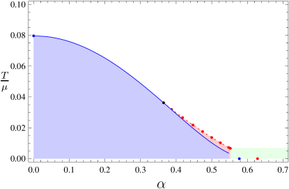
Figure 8: Phase structure of the p-wave superconductor theory: In the blue and red region the broken phase is the thermodynamically preferred phase, while in the white region the Reissner-Nordström black hole is the ground state. In the blue region the Reissner-Nordström black hole is unstable and the transition from the white to the blue region is second order. In the red region the Reissner-Nordström black hole is still stable. The transition form the white to the red region is first order. The black dot determines the critical point where the order of the phase transition changes. In the green region we cannot trust our numerics.

Let us now discuss the phase structure of this theory. At temperature below the critical temperature the thermodynamically favored phase is the holographic superfluid. By varying the parameter $\alpha$, the critical temperature changes. In addition in [43] it was found that the order of the phase transition depends on the ratio of the coupling constants $\alpha$. For $\alpha\leq\alpha_{c}=0.365$, the phase transition is second order while for larger values of $\alpha$ the transition becomes first order. The critical temperature decreases as we increase the parameter $\alpha$. The quantitative dependence of the critical temperature on the parameter $\alpha$ is given in Figure 8. The broken phase is thermodynamically preferred in the blue and red region while in the white region the Reissner-Nordström black hole is favored. The Reissner-Nordström black hole is unstable in the blue region and the phase transition from the white to the blue region is second order. In the red region, the Reissner-Nordström black hole is still stable however the state with non-zero condensate is preferred. The transition from the white to the red region is first order. In the green region we cannot trust our numerics. At zero temperature, the data is obtained as described in [52, 53].

4.3 Diffusion Constants

We now determine the diffusion constants at the critical temperature. Since the system is still described by a Reissner-Nordström black hole as in the holographic s-wave superfluid and thus the equations of motion for the fluctuations coincide, we can use the same expressions to calculate the diffusion constants for the holographic p-wave superfluid. The only change is the dependence of the critical temperature on the parameter $\alpha$. The numerical results are shown in Figure 9. Comparing the phase diagram of Figure 8 and the diffusion constants of Figure 9, we see that they are virtually identical. Furthermore, the analytical expression converting the curve of critical values of $\nicefrac{{T}}{{\mu}}$ into the product $D(T_{c})T_{c}$ is the same for both holographic superconductors. Thus, it is not surprising that we will find answers that have a very large resemblance. Moreover, the same is true for the s-wave superconductors and the comparison between the s-wave and the p-wave superconductor: All curves for $D(T_{c})T_{c}$ are very similar in both cases. In the following section we will give a detailed conclusion and explain some possible mechanisms which may lead to the decrease of $D(T_{c})T_{c}$ in the backreacted case.

      

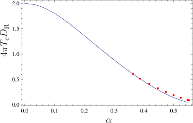
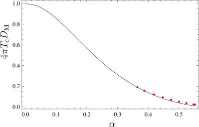
Figure 9: $C_{R}=4\pi T_{c}D_{R}(T_{c})$ and $C_{M}=4\pi T_{c}D_{M}(T_{c})$ related to charge diffusion $D_{\mathrm{R}}$ and momentum diffusion $D_{\mathrm{M}}$ depending on the strength of the backreaction $\alpha$ for the holographic p-wave superfluid with $d=4$. The blue line corresponds to the constants evaluated at the temperature at which the Reissner-Nordström black hole becomes unstable (see blue line in Figure 8). The red dots corresponds to the constants evaluated at the critical temperature at which the superfluid phase is thermodynamically preferred (see red dots in Figure 8).

5 Conclusions

Let us summarize the main results of our paper: Motivated by Homes’ law we have analyzed the diffusion constants in holographic s- and p-wave superconductors with backreaction. In particular we have discussed the temperature and density dependence of the momentum and R-charge diffusion for various masses of the scalar field (in the s-wave case) and for different strengths of the backreaction. We have found that the diffusion constants decrease with increasing backreaction and that the decay of the diffusion constants increases with increasing mass of the scalar field. For non-negative masses of the s-wave superconductor scalar field, we find an emerging $\text{AdS}_{2}$ at zero temperature which defines a critical strength of the backreaction $\alpha_{c}$. Above this critical backreaction there is no phase transition to the superfluid/condensed phase, thus implying that $\alpha_{c}$ defines a quantum phase transition between the normal and the condensed phase. These results are of intrinsic interest within holography.
Let us now discuss these results in relation to Homes’ law: We have found that without backreaction, holographic superconductors obey Homes’ law since $\tau_{c}T_{c}=\text{const.}$ in all spacetime dimensions greater than two. In the case of s-wave superconductors, this holds for all scalar field masses. Without backreaction, the result $\tau_{c}T_{c}=\text{const.}$ is almost automatic since the diffusion constant $D$ scales as $1/T$. Turning on the backreaction, we find that $D(T_{c})T_{c}$ is no longer constant, but decreases with increasing backreaction strength. Both for s-wave and p-wave holographic superconductors, we obtain virtually the same curves for the various diffusion constants in three and four dimensions. In particular, the s-wave superconductor shows this behavior in three and four dimensions for different masses of the scalar field. This is a strong indication that there is a universal principle at work, although we do not find a true constant. There are several possibilities how corrections may arise:

1. The simplest explanation is the fact that we cannot assume the validity of the assumption (17) for holographic superconductors. As discussed at the end of Section 3.5, increasing the backreaction $\alpha$ leads to the formation of a pseudo-gap and there are normal state charge carriers present in the superconducting phase as well. The dependence of the pseudo-gap on the backreaction has been studied holographically in [54] where it was found that the pseudo-gap arising in the superconducting phase becomes larger with increasing backreaction, as clearly visible in Figure 4 of [54]. Assuming that the Ferrell-Glover-Tinkham sum rule (12) is still valid in the presence of the pseudo-gap, $N_{\text{s}}$ in (12) is no longer zero. This leads to correction terms to (17) and (22),

   $$\omega_{\text{Ps}}^{2} =\omega_{\text{Pn}}^{2}-8N_{\text{s}} \Leftrightarrow \qquad\tau_{c}T_{c} =\frac{4\pi}{C}\left(1-\frac{N_{\text{s}}}{N_{\text{n}}}\right).$$ (82)

   Thus, we would expect the “constant” in (26) to decrease and this is exactly what we see in Figure 5, 6, 7 and 9.

2. Even more dramatically, the sum rule (12) may not be valid for holographic superconductors in the presence of the backreaction. In this case Homes’ law will be implied by Tanner’s law (18) which applies to high $T_{c}$ superconductors. It would be interesting to study Tanner’s law in a holographic context (regardless of its relevance to Homes’ law). Our result leads to the conjecture that the relation between the superconducting charge carrier and the normal state charge carrier concentration is dependent on the strength of the backreaction

   $$n_{\text{s}} =B(\alpha)n_{\text{n}},$$ (83)

   such that (26) is modified by the monotonically decreasing function $$B(\alpha)$$ yielding

   $$\tau_{c}T_{c} =4\pi\frac{B(\alpha)}{C}.$$ (84)

3. The proportionality between the time scale and the diffusion constant could in principle depend on $\alpha$ and $\bar{Q}$, i.e. a function $A(\alpha)$, say. In this case the question arises if there might be some additional dynamics concerning diffusion in holographic superfluids/superconductors which would have to be taken into account. This would lead to the modified version of (27),

   $$D(T_{c})T_{c}=\frac{4\pi}{A(\alpha)C}.$$ (85)

4. From a condensed matter point of view, we should look at the dominant time scale which is given by the energy relaxation time. This needs not necessarily to be the same as the momentum time scale. However, the Einstein-Higgs models obey relativistic symmetries and therefore the momentum diffusion/time scales are related to the energy diffusion/time scales. In fact, the energy diffusion constant is identical to the momentum diffusion as expected from the symmetries, up to a factor depending on the spacetime dimensions: Conformal symmetry implies that the bulk viscosity vanishes, which ensures that hydrodynamic modes corresponding to energy and momentum diffusion are related. So the natural choice is indeed to look at momentum and R-charge diffusive processes to determine the relevant time scales, as done in this paper. Nevertheless, this issue deserves further investigation.

5. A more speculative and interesting correction could originate from the fact that we already have an infinite Drude peak in the normal phase indicating an ideal conductor, i.e. $\operatorname{Re}\sigma(\omega)\propto\delta(\omega)$, since there is no lattice present in our model. Entering the superconducting phase seems to add additional spectral weight due to the condensation of the scalar field. This in turn implies that the perfect conducting metal in the normal state does not turn into a superconductor but that the ideal conductor and the superconductor coexist in the superconducting phase. Here we would again expect a violation of equal spectral weight, or of the Ferrell-Glover-Tinkham sum rule (12), as well as having a simple relation between the normal state charge carrier concentration and the one in the superconducting state. In order to really understand what happens in the superconducting phase, one needs to determine the behavior of $\rho_{\text{s}}$ for small temperatures and to check that only the contribution to the superconducting state is considered. It is believed that exactly at $T=0$ the normal state delta shaped Drude peak vanishes and the coefficient of the delta distribution is really the superfluid strength, yet this is not explicitly shown so far to our knowledge.

6 Outlook

As is explained in Section 5, the most striking explanation for corrections to $\tau_{c}T_{c}=\text{const.}$ in the backreacting case comes from additional degrees of freedom in the pseudo-gap. Let us give a list of open questions which needs to be addressed to make further progress:

• An explicit calculation to verify the validity of the sum rules of holographic superconductors is in itself an interesting question. Therefore one needs to calculate the superfluid density including its dependence on the backreaction at zero temperature as well as the optical conductivity above the critical temperature and near zero temperature. The conceptual setting is quite clear, but the numerical implementation might be challenging.

• In order to confirm the assumptions made in (18) one needs to check if the holographic superconductors show a relation between $n_{\text{s}}$ and $n_{\text{n}}$, i.e. Tanner’s law. The same challenges might arise as in the aforementioned point.

• It would be interesting to understand if the holographic superconductors consists of an ideal metal coexisting with a superconductor following the speculative point 5 made in the conclusion. If so, one needs to devise a scheme to calculate the superfluid strength by removing the influence of the perfectly conducting metal. There are several ways to achieve this: First of all it would be interesting to look for the Meißner-Ochsenfeld effect, i.e. to calculate the transversal response of the gauge field which is only sensitive to the superfluid strength deep in the superconducting phase. Alternatively, a further idea is to change the geometry such that the degrees of freedom of the normal state become very massive and are thus “gapped out” of the spectrum. Possible candidates are the hard-wall geometry, studied in the condensed matter context in [55], or a more smooth realization emerging in the AdS-soliton solutions [56], focusing in particular on the AdS-soliton to AdS-soliton superconductor transition. A suppression of normal low energy spectral weight has also been observed recently in a different context in [57]. It will also be interesting to consider holographic systems with lattice structure, such as [17] and [18], in the context explained here. These do not have the $\delta$-peak in the normal phase, as expected for a system with an underlying lattice.

• Since within condensed matter physics, energy diffusion is relevant to Homes’ law, a systematic investigation of the relation between energy diffusion and momentum diffusion in the holographic context appears to be highly desirable, in particular in the presence of finite density and backreaction. As explained in the conclusion, our assumption that energy and momentum diffusion are related within holography is well-motivated. Nevertheless this is a crucial issue which requires systematic study.

• It would also be useful to calculate the dependence of fermionic excitations on the backreaction, for instance by generalizing the work of [53] and [58].

In any case it is very important to disentangle the different contributions to the $\delta$-peak in the superconducting phase in order to learn the differences which arise in holographic superfluids/superconductors as compared to “real world” systems.

Appendices

Appendix A Plasma-Frequency

Here we give a brief overview over the plasma frequency and the relations to the dielectric function and its role in terms of the superfluid density. Formally, the plasma frequency is defined as

$$\frac{\omega_{\text{P}}^{2}}{8}=\int_{0}^{\infty}\operatorname{d\mathit{\omega}}\operatorname{Re}\sigma(\omega),$$ (86)

using the optical sum rule. Using the relations between the complex dielectric function $\epsilon(\omega)$ and the complex optical conductivity $\sigma(\omega)$,

$$\epsilon =\epsilon_{\infty}+\frac{4\pi\mathrm{i}}{\omega}\sigma(\omega) \Rightarrow \qquad\operatorname{Re}\sigma(\omega) =\frac{\omega}{4\pi}\operatorname{Im}\epsilon(\omega),$$ (87)

we may rewrite the plasma frequency in terms of the dielectric function as

$$\omega_{\text{P}}^{2}=\frac{2}{\pi}\int_{0}^{\infty}\operatorname{d\mathit{\omega}}\omega\operatorname{Im}\epsilon(\omega).$$ (88)

With the help of the Kramers-Kronig relation for non-negative frequencies

$$\operatorname{Re}f(\omega) =\frac{2}{\pi}\mathcal{P}\int_{0}^{\infty}\operatorname{d\mathit{\omega}}^{\prime}\frac{\omega^{\prime}\operatorname{Im}f(\omega^{\prime})}{\omega^{\prime 2}-\omega^{2}}, \operatorname{Im}f(\omega) =-\frac{2\omega}{\pi}\mathcal{P}\int_{0}^{\infty}\operatorname{d\mathit{\omega}}^{\prime}\frac{\operatorname{Re}f(\omega^{\prime})}{\omega^{\prime 2}-\omega^{2}},$$ (89)

we may relate $\operatorname{Im}\epsilon(\omega)$ to $\operatorname{Re}\epsilon(\omega)-1$. Note that for the dielectric function the polarization $P(\omega)$ is the response to the applied electric field $E(\omega)$,

$$4\pi P(\omega)=\left(\epsilon(\omega)-1\right)E(\omega).$$ (90)

Therefore a convenient form to write the Kramers-Kronig relation for the dielectric function is to include the additional $-1$ in the real part of $\epsilon(\omega)$,

$$\operatorname{Re}\epsilon(\omega)-1 =\frac{2}{\pi}\mathcal{P}\int_{0}^{\infty}\operatorname{d\mathit{\omega}}^{\prime}\frac{\omega^{\prime}\operatorname{Im}\epsilon(\omega^{\prime})}{\omega^{\prime 2}-\omega^{2}}=-\frac{2}{\pi}\frac{1}{\omega^{2}}\mathcal{P}\int_{0}^{\infty}\operatorname{d\mathit{\omega}}^{\prime}\frac{\omega^{\prime}\operatorname{Im}\epsilon(\omega^{\prime})}{1-\frac{\omega^{\prime 2}}{\omega^{2}}}$$

$$\overset{\omega\gg\omega^{\prime}}{=}-\frac{2}{\pi}\frac{1}{\omega^{2}}\int_{0}^{\infty}\operatorname{d\mathit{\omega}}^{\prime}\omega^{\prime}\operatorname{Im}\epsilon(\omega^{\prime})=-\frac{\omega_{\text{P}}^{2}}{\omega^{2}},$$ (91)

where we are interested in the high frequency regime ($\omega\gg\nicefrac{{1}}{{\tau}}$) since the sum rule is strictly valid only for $\omega\to\infty$. In experiments we deal with finite frequencies only, and thus it is possible to extract the plasma frequency by the following extrapolation of experimental data,

$$\omega_{\text{P}}^{2}=\lim_{\omega\to 0}\left(-\omega^{2}\operatorname{Re}\epsilon(\omega)\right).$$ (92)

As explained in the main text the superconducting plasma frequency determines the frequency above which the superconductors becomes “transparent” in analogy with the normal metal plasma frequency. The reason for this terminology follows from the fact that photons can only penetrate the superconductor for length scales smaller than the London penetration depth $\lambda_{\text{L}}$ which corresponds to $\omega_{\text{Ps}}$. Here, the superconducting plasma frequency should be understood with the aforementioned analogy to normal metals in mind, described by the Drude-Sommerfeld form of the optical conductivity (102). In this case the (superconducting) plasma frequency is given by

$$\omega_{\text{Ps}}^{2}=8\frac{ne^{2}}{m}\int_{0}^{\infty}\operatorname{d\mathit{(\omega\tau)}}\frac{1}{1+(\omega\tau)^{2}}=8\frac{ne^{2}}{m}\arctan(\omega\tau)\Big{|}_{0}^{\infty}=4\pi\frac{ne^{2}}{m}=\lambda_{\text{L}}^{-2}.$$ (93)

Experimentally, we cannot reach infinite frequencies and thus the sum rule is modified by a cut-off frequency $\omega_{c}$, sometimes called the partial optical sum rule of the Drude-Sommerfeld form

$$\int_{0}^{\omega_{\text{c}}}\operatorname{d\mathit{(\omega\tau)}}\frac{1}{1+(\omega\tau)^{2}}=8\frac{ne^{2}}{m}\arctan(\omega\tau)\Big{|}_{0}^{\omega_{\text{c}}}=\frac{\omega_{\text{P}}^{2}}{4\pi}\arctan(\omega_{\text{c}}\tau).$$ (94)

Expanding the inverse tangent function for $\omega_{c}\to\infty$, we get a series expansion in the relaxation rate $\nicefrac{{1}}{{\tau}}$ which reads

$$\arctan\left(\omega_{\text{c}}\tau\right) =\frac{\pi}{2}-\frac{1}{\omega_{\text{c}}\tau}+\mathcal{O}\left(\frac{1}{\omega_{\text{c}}^{3}\tau^{3}}\right),$$ (95)

and thus

$$\int_{0}^{\omega_{\text{c}}}\operatorname{d\mathit{\omega}}\operatorname{Re}\sigma(\omega) \approx\frac{\omega_{\text{P}}^{2}}{8}\left(1-\frac{2}{\pi}\frac{1}{\omega_{\text{c}}\tau}\right),$$ (96)

from which we recover (86) for $\omega_{\text{c}}\to\infty$.

Appendix B Drude-Sommerfeld Model

In the previous sections we made use of some facts of Drude-Sommerfeld theory, which we now discuss in some detail. The original Drude model is a purely classical model describing a gas of electrons diffusing through a fixed lattice of ions. These generate a positively charge background to balance the negative charge of the electron gas. Even after the discovery of quantum mechanics, the Drude model can still be used but some modifications are needed: The electrons are described by a fermionic gas obeying Fermi-Dirac statistics. This extension of the original model is usually called Drude-Sommerfeld model. There are several ways to arrive at the Drude formula used in (20) each with their own set of approximations. Essentially, there are three approaches:

1. A classical approach assuming the existence of an average relaxation time describing the relaxation to equilibrium after turning off an external electric field, i.e. the relaxation time approximation which operationally replaces the collision integral by a linearized approximation including only the relaxation time scale and the Maxwell-Boltzmann distribution in the kinetic/Boltzmann transport equation. Strictly speaking, this derivation is borrowed from hydrodynamics where the collisions refer to a gas of weakly interacting particles.

2. A semi-classical approach taking into account the quantum nature of the electron gas. Thus the free mean path is determined by the Fermi velocity of the electrons $\ell=v_{\text{F}}\tau$ and only electrons near the Fermi surface can participate.

3. A full microscopic approach considering an interacting electron gas employing Fermi liquid theory in combination with a diagrammatic expansion (and additional approximations such as the random phase approximation). Here the assumptions of Fermi liquid theory, in particular adiabatic continuity, are needed. Furthermore, it is useful to introduce an effective frequency dependent mass $m^{*}(\omega)$ for the quasi-particles of Fermi liquid theory incorporating the effects of electron-phonon and electron-electron interactions as well as a frequency dependent effective time scale $\tau^{*}(\omega)$. However, in the case of impurity scattering the ratio $\nicefrac{{\tau^{*}}}{{m^{*}}}$ is identical to the bare values since the renormalization of the lifetime cancels the renormalization of the mass. This can be explicitly seen in a diagrammatic calculation of the current-current correlator using the Kubo formula. Here the mass renormalization cancels since the diagrams included in the self-energy are also included in the two particle diagrams. This is in agreement with Fermi liquid theory stating that the current of the quasi particles is independent of the interaction.

Since we do not know in general if there are really quasi-particles involved in strongly correlated systems (apart from heavy Fermi liquids), it seems to be a good strategy not attempt to explain Homes’ law microscopically, but to take the “effective field theory” philosophy that focuses on the macroscopic rather than the microscopic degrees of freedom. In particular dealing with “Planckian dissipation” there is no particle transport and we are primarily interested in quantum critical transport at finite density. Therefore we may follow the standard derivation using the Kubo formula without resorting to the aforementioned technicalities. A nice exposition of this derivation can be found in [59]. Here we will just state the main ideas and the result. We start with an interaction Hamiltonian

$$\mathcal{H}_{\text{int}}=-\frac{1}{c}\mathbfit{J}\bm{\cdot}\mathbfit{A},$$ (97)

and use the Kubo formula for the conductivity,

$$\sigma(\omega,\mathbfit{k})=\sum_{s}\frac{1}{\hbar\omega}\int\operatorname{d\mathit{t}}\left\langle s\middle|\>\mathbfit{J}(0,\mathbfit{k})\bm{\cdot}\mathbfit{J}(t,\mathbfit{k})^{\ast}\>\middle|s\right\rangle\,\mathrm{e}^{-\mathrm{i}\omega t}\,.$$ (98)

The current density operator $\mathbfit{J}$ can be rewritten in terms of the momentum operator. Assuming an exponential decay with a single time scale for all current-current correlators (relaxation time approximation) and the dipole approximation (the external electric field is constant over the characteristic length scale which is surely valid for $v_{\text{F}}\ll c$) we arrive at

$$\sigma(\omega)=\frac{e^{2}\tau}{m^{*}}\frac{f}{1-\mathrm{i}\omega\tau},$$ (99)

where $f$ describes the oscillator strength measuring the transition probability between two states given by

$$f=2\sum_{j,s,s^{\prime}}\frac{\left\lvert\left\langle s\middle|\>\mathbfit{p}_{j}\>\middle|s^{\prime}\right\rangle\right\rvert^{2}}{m^{*}\hbar(\omega_{s}-\omega_{s^{\prime}})}.$$ (100)

Furthermore the oscillator strength can be evaluated under the assumption of free electrons i.e.

$$m^{*}\hbar(\omega_{s}-\omega_{s^{\prime}}) =\frac{\hbar^{2}\mathbfit{k}^{2}}{2} \qquad\sum_{s,s^{\prime}}\left\lvert\left\langle s\middle|\>\mathbfit{p}_{j}\>\middle|s^{\prime}\right\rangle\right\rvert^{2} =\left\langle\mathbfit{p}_{j}^{2}\right\rangle=\frac{\hbar^{2}\mathbfit{k}^{2}}{4},$$ and (101)

since the self-interaction or electron-lattice interactions are already taken care of in the renormalization of the mass $m^{*}(\omega)$ and the relaxation rate $\tau^{-1}(\omega)=\tau^{-1}_{\text{impurity}}+\tau^{-1}_{\text{el-ph}}+\tau^{-1}_{\text{el-el}}$. Inserting (101) into (100) the oscillator strength $f$ is given by the electron (or charge carrier) density $n$ and thus

$$\sigma(\omega)=\frac{ne^{2}\tau}{m^{*}}\frac{1}{1-\mathrm{i}\omega\tau}=\frac{\omega_{\text{p}}^{2}}{4\pi}\frac{1}{\frac{1}{\tau}-\mathrm{i}\omega},$$ (102)

using the definition of the plasma frequency (7) which in the limit of $\omega\to 0$ reduces to (20). If we assume the correction of $\tau_{\text{el-ph}}$ and $\tau_{\text{el-el}}$ to be small compared to $\tau_{\text{impurity}}$ we can follow the reasoning presented in point 3 and replace $\nicefrac{{\tau^{*}}}{{m^{*}}}$ by $\nicefrac{{\tau}}{{m}}$. The maximum of the real part of the optical conductivity (102) at $\omega=0$ is called the Drude peak, whereas the imaginary part shows a maximum at $\omega=\nicefrac{{1}}{{\tau}}$.

Appendix C Equations of Motion for the s–Wave Fluctuations

First we expand the matter Lagrangian up to quadratic order in the fluctuations

$$\mathcal{L}^{(0)}_{cd} =-\left(\nabla_{c}\Phi+\mathrm{i}A_{c}\Phi\right)\left(\nabla_{d}\Phi-\mathrm{i}A_{d}\Phi\right)-m^{2}\Phi^{2},$$ (103)

$$\mathcal{L}^{(1)}_{cd} =-\nabla_{c}\delta\phi^{\ast}\nabla_{d}\Phi-\nabla_{d}\delta\phi\nabla_{c}\Phi+\mathrm{i}\nabla_{c}\Phi A_{d}\delta\phi-\mathrm{i}\nabla_{d}\Phi A_{c}\delta\phi^{\ast}-\mathrm{i}A_{c}\nabla_{d}\delta\psi\Phi$$

$$\hskip 12.0pt+\mathrm{i}A_{d}\nabla_{c}\delta\phi^{\ast}\Phi-A_{c}A_{d}\Phi\left(\delta\phi+\delta\phi^{\ast}\right)-\left(A_{c}a_{d}+A_{d}a_{c}\right)\Phi^{2}-m^{2}\Phi\left(\delta\phi+\delta\phi^{\ast}\right),$$

$$\mathcal{L}^{(2)}_{cd} =-\nabla_{c}\delta\phi\nabla_{d}\delta\phi^{\ast}-\mathrm{i}A_{c}\nabla_{d}\delta\phi\delta\phi^{\ast}+\mathrm{i}A_{d}\nabla_{c}\delta\phi^{\ast}\delta\phi-\mathrm{i}a_{c}\nabla_{d}\delta\phi\Phi+\mathrm{i}a_{d}\nabla_{c}\delta\phi^{\ast}\Phi$$

$$\hskip 12.0pt+\mathrm{i}\nabla_{c}\Phi a_{d}\delta\phi-\mathrm{i}\nabla_{d}\Phi a_{c}\delta\phi^{\ast}-A_{c}A_{d}\delta\phi\delta\phi^{\ast}-\left(A_{c}a_{d}+A_{d}a_{c}\right)(\delta\phi+\delta\phi^{\ast})$$

$$\hskip 12.0pt-a_{a}a_{b}\Psi^{2}-m^{2}\delta\phi^{\ast}\delta\phi,$$

as well as the Maxwell Lagrangian

$$\mathcal{L}_{\text{M}}^{(1)}=\alpha^{2}L^{2}\sqrt{-G}\left[-\frac{1}{4}G^{ce}G^{df}\left(F_{cd}\delta F_{ef}+\delta F_{cd}F_{ef}\right)+G^{cd}\mathcal{L}^{(2)}_{cd}\right.\\[6.0pt] -\frac{1}{4}\left(G^{cs}G^{et}h_{st}G^{df}+G^{ds}G^{ft}h_{st}G^{ce}+\frac{1}{2}G^{st}h_{st}G^{ce}G^{df}\right)F_{cd}F_{ef}\\[6.0pt] \left.+\left(G^{cs}G^{dt}h_{st}+\frac{1}{2}G^{st}h_{st}G^{cd}\right)\mathcal{L}^{(0)}_{cd}\right],$$ (104)

$$\mathcal{L}_{\text{M}}^{(2)}=\alpha^{2}L^{2}\sqrt{-G}\left\{-\frac{1}{4}G^{ce}G^{df}\delta F_{cd}\delta F_{ef}+G^{cd}\mathcal{L}^{(2)}_{cd}\right.\\[6.0pt] -\frac{1}{4}\left(G^{cs}G^{et}h_{st}G^{df}+G^{ds}G^{ft}h_{st}G^{ce}+\frac{1}{2}G^{st}h_{st}G^{ce}G^{df}\right)\left(F_{cd}\delta F_{ef}+\delta F_{cd}F_{ef}\right)\\[6.0pt] +\left(G^{cs}G^{dt}h_{st}+\frac{1}{2}G^{st}h_{st}G^{cd}\right)\mathcal{L}^{(1)}_{cd}\\[6.0pt] -\frac{1}{4}\left[G^{cs}G^{et}h_{st}G^{dm}g^{fn}h_{mn}+\frac{1}{2}G^{mn}h_{mn}\left(G^{cs}G^{et}h_{st}G^{df}+G^{ds}G^{ft}h_{st}g^{ce}\right)\right.\\[6.0pt] +\left.\left(\frac{1}{8}g^{st}G^{mn}-\frac{1}{4}G^{tm}G^{sn}\right)h_{st}h_{mn}G^{ce}G^{df}\right]F_{ce}F_{df}\\[6.0pt] +\left.\left[\frac{1}{2}G^{st}h_{st}G^{cm}G^{dn}h_{mn}+\left(\frac{1}{8}G^{st}G^{mn}h_{st}h_{mn}-\frac{1}{4}G^{tm}G^{sn}\right)h_{st}h_{mn}G^{cd}\right]\mathcal{L}^{(0)}_{cd}\right\}.$$ (105)

The corresponding equations of motion for the scalar fluctuations are involved expressions so we will simplify them according to our needs. Since we are working in the normal phase we can set $\Phi(u)\equiv 0$. Furthermore, the only non-vanishing component of the background gauge field is $A_{t}(u)$ with all other components being zero. In order to work out the quasi-normal modes we apply a Fourier transformation and assume plain wave behavior for the spatial dependence

$$\delta\phi(t,\mathbfit{x},u) =\int\frac{\operatorname{d\mathit{\omega}}\operatorname{d^{\mathit{d}--1}\mathit{\mathbfit{k}}}}{(2\pi)^{d}}\,\mathrm{e}^{-\mathrm{i}\omega t+\mathrm{i}\mathbfit{k}\bm{\cdot}\mathbfit{x}}\,\delta\phi(u),$$ (106)

$$a_{a}(t,\mathbfit{x},u) =\int\frac{\operatorname{d\mathit{\omega}}\operatorname{d^{\mathit{d}--1}\mathit{\mathbfit{k}}}}{(2\pi)^{d}}\,\mathrm{e}^{-\mathrm{i}\omega t+\mathrm{i}\mathbfit{k}\bm{\cdot}\mathbfit{x}}\,a_{a}(u),$$

$$h_{ab}(t,\mathbfit{x},u) =\int\frac{\operatorname{d\mathit{\omega}}\operatorname{d^{\mathit{d}--1}\mathit{\mathbfit{k}}}}{(2\pi)^{d}}\,\mathrm{e}^{-\mathrm{i}\omega t+\mathrm{i}\mathbfit{k}\bm{\cdot}\mathbfit{x}}\,h_{ab}(u).$$

Thus, we end up with the following equation of motion for the scalar fluctuations

$$\delta\phi^{\prime\prime}(u)+\left(\frac{f^{\prime}(u)}{f(u)}-\frac{d-1}{u}\right)\delta\phi^{\prime}(u)+\left[\frac{(\omega+A_{t})^{2}}{f(u)^{2}}-\frac{\mathbfit{k}^{2}}{f(u)}-\frac{L^{2}m^{2}}{u^{2}f(u)}\right]\delta\phi(u)=0,$$ (107)

and for the gauge field fluctuations we have

$$a_{t}^{\prime\prime}(u)-\frac{d-3}{u}a_{t}^{\prime}(u)-\left(\frac{\mathbfit{k}^{2}}{f(u)}\right)a_{t}(u)-\frac{\omega}{f(u)}\mathbfit{k}\bm{\cdot}\mathbfit{a}(u)+\mathrm{i}\omega\left(a_{u}^{\prime}(u)-\frac{d-3}{u}a_{u}(u)\right)\\[6.0pt] -\frac{3u^{2}A_{t}^{\prime}(u)}{2L^{2}f(u)}h_{tt}^{\prime}(u)+\frac{u^{2}A_{t}^{\prime}(u)}{2L^{2}}\sum_{i=1}^{d-1}h_{ii}^{\prime}(u)+\frac{3u^{2}f(u)A_{t}^{\prime}(u)}{2L^{2}}h_{uu}^{\prime}(u)\\[6.0pt] +\frac{u}{L^{2}}A_{t}^{\prime}(u)\sum_{i=1}^{d-1}h_{ii}(u)+\frac{\mathrm{i}uA_{t}^{\prime}(u)}{L^{2}}\sum_{i=1}^{d-1}h_{ui}(u)k_{i}+\frac{3}{2}\frac{u^{2}f(u)}{L^{2}}\left(\frac{f^{\prime}(u)}{f(u)}+\frac{2}{u}\right)A_{t}^{\prime}(u)h_{uu}(u)=0,$$ (108)

$$\mathbfit{a}^{\prime\prime}(u)+\left(\frac{f^{\prime}(u)}{f(u)}-\frac{d-3}{u}\right)\mathbfit{a}^{\prime}(u)+\left(\frac{\omega^{2}}{f(u)^{2}}-\frac{\mathbfit{k}_{\perp}^{2}}{f(u)}\right)\mathbfit{a}(u)+\frac{\mathbfit{k}}{f(u)}\big{(}\mathbfit{k}_{\perp}\bm{\cdot}\mathbfit{a}(u)\big{)}\\[6.0pt] +\frac{\omega\mathbfit{k}}{f(u)^{2}}a_{t}(u)-\mathrm{i}\mathbfit{k}\left[a^{\prime}_{u}(u)+\left(\frac{f^{\prime}(u)}{f(u)}-\frac{d-3}{u}\right)a_{u}(u)\right]\\[6.0pt] -\frac{u^{2}A_{t}^{\prime}(u)}{L^{2}f(u)}\mathbfit{h}_{t}^{\prime}(u)-\frac{2uA_{t}^{\prime}(u)}{L^{2}f(u)}\mathbfit{h}_{t}(u)-\frac{\mathrm{i}u^{2}\omega A_{t}^{\prime}(u)}{L^{2}f(u)}\mathbfit{h}_{u}(u)=0,$$ (109)

$$\frac{\omega}{f(u)}a_{t}^{\prime}(u)+\mathbfit{k}\bm{\cdot}\mathbfit{a}^{\prime}(u)-\mathrm{i}\left(\mathbfit{k}^{2}-\frac{\omega^{2}}{f(u)}\right)a_{u}(u)\\[6.0pt] -\frac{3}{2}\frac{u^{2}\omega A_{t}^{\prime}(u)}{L^{2}f(u)^{2}}h_{tt}(u)-\frac{u^{2}A_{t}^{\prime}(u)}{L^{2}f(u)}\sum_{i=1}^{d-1}h_{ti}k_{i}+\frac{u^{2}\omega A_{t}^{\prime}(u)}{2L^{2}f(u)}\sum_{i=1}^{d-1}h_{ii}(u)+\frac{3}{2}\frac{u^{2}\omega A_{t}^{\prime}(u)}{L^{2}}h_{uu}(u)=0.$$ (110)

where $\mathbfit{h}_{t}(u),\mathbfit{h}_{u}(u)$ denotes the spatial entries of the corresponding row/column and $\mathbfit{k}_{\perp}$ denotes the transverse vector orthogonal to the directions given by the particular equations for the component of $\mathbfit{a}(u)$. For instance, we can look at the equation for one of the $d-1$ spatial components, $\mathbfit{a}(u)=a_{x}(u)\mathbfit{e}_{x}$ say, so $\mathbfit{k}_{\perp}=k_{y}\mathbfit{e}_{y}+k_{z}\mathbfit{e}_{z}+\dotsm$ and hence $\mathbfit{k}_{\perp}\bm{\cdot}\mathbfit{a}$ couples the complementary components to the one chosen, i.e. $a_{y}(u),a_{z}(u),\dotsc$. Furthermore, assuming $\mathbfit{k}=k_{x}\mathbfit{e}_{x}$ , we see that the equations of the $a_{x}(u)$ component couples only with the $a_{t}(u)$ component (in this case $\mathbfit{k}_{\perp}=\mathbfit{0}$), whereas the equations for all other $d-2$ spatial components decouple. Looking at the transverse directions e.g. $\mathbfit{k}=k_{y}\mathbfit{e}_{y}+k_{z}\mathbfit{e}_{z}+\dotsm$, the equation for the fluctuations in the $x$-direction will decouple from all other $d-2$, but the equations for the remaining $d-2$ fluctuations will couple with each other and $a_{t}(u)$.

References

- [1] P. Kovtun, D. T. Son and A. O. Starinets, Holography and Hydrodynamics: Diffusion on Stretched Horizons, JHEP 0310 (2003) 064 [hep-th/0309213].
- [2] A. Buchel and J. T. Liu, Universality of the Shear Viscosity in Supergravity, Phys.Rev.Lett. 93 (2004) 090602 [hep-th/0311175].
- [3] P. Kovtun, D. Son and A. Starinets, Viscosity in Strongly Interacting Quantum Field Theories from Black Hole Physics, Phys.Rev.Lett. 94 (2005) 111601 [hep-th/0405231].
- [4] N. Iqbal and H. Liu, Universality of the Hydrodynamic Limit in AdS/CFT and the Membrane Paradigm, Phys.Rev. D79 (2009) 025023 [0809.3808].
- [5] A. Sinha and R. C. Myers, The Viscosity Bound in String Theory, Nucl.Phys. A830 (2009) 295C–298C [0907.4798].
- [6] J. Erdmenger, P. Kerner and H. Zeller, Non-universal shear viscosity from Einstein gravity, Phys.Lett. B699 (2011) 301–304 [1011.5912].
- [7] J. Erdmenger, P. Kerner and H. Zeller, Transport in Anisotropic Superfluids: A Holographic Description, JHEP 1201 (2012) 059 [1110.0007].
- [8] A. Rebhan and D. Steineder, Violation of the Holographic Viscosity Bound in a Strongly Coupled Anisotropic Plasma, Phys.Rev.Lett. 108 (2012) 021601 [1110.6825].
- [9] H. Liu, J. McGreevy and D. Vegh, Non-Fermi liquids from holography, Phys.Rev. D83 (2011) 065029 [0903.2477].
- [10] M. Cubrovic, J. Zaanen and K. Schalm, String Theory, Quantum Phase Transitions and the Emergent Fermi-Liquid, Science 325 (2009) 439–444 [0904.1993].
- [11] N. Iqbal, H. Liu and M. Mezei, Lectures on Holographic Non-Fermi Liquids and Quantum Phase Transitions, 1110.3814.
- [12] S. A. Hartnoll, Lectures on Holographic Methods for Condensed Matter Physics, Class.Quant.Grav. 26 (2009) 224002 [0903.3246].
- [13] C. P. Herzog, Lectures on Holographic Superfluidity and Superconductivity, J.Phys.A A42 (2009) 343001 [0904.1975]. 39 pages, 9 figures, lectures given at the Trieste Spring School on Superstring Theory and Related Topics.
- [14] G. T. Horowitz, Introduction to Holographic Superconductors, 1002.1722.
- [15] M. Kaminski, Flavor Superconductivity & Superfluidity, Lect.Notes Phys. 828 (2011) 349–393 [1002.4886].
- [16] J.-H. She, B. J. Overbosch, Y.-W. Sun, Y. Liu, K. Schalm, J. A. Mydosh and J. Zaanen, Observing the Origin of Superconductivity in Quantum Critical Metals, Phys.Rev. B84 (2011) 144527 [1105.5377].
- [17] G. T. Horowitz, J. E. Santos and D. Tong, Optical Conductivity with Holographic Lattices, JHEP 1207 (2012) 168 [1204.0519].
- [18] Y. Liu, K. Schalm, Y.-W. Sun and J. Zaanen, Lattice Potentials and Fermions in Holographic Non Fermi-Liquids: Hybridizing Local Quantum Criticality, 1205.5227.
- [19] S. Sachdev, Quantum Phase Transition. Cambridge University Press, 2011.
- [20] S. Sachdev and B. Keimer, Quantum Criticality, Phys.Today 64N2 (2011) 29 [1102.4628].
- [21] J. Zaanen, Superconductivity: Why the Temperature is High, Nature 430 (Jul, 2004) 512–513.
- [22] M. Ammon, Gauge/Gravity Duality Applied to Condensed Matter Systems, Fortsch.Phys. 58 (2010) 1123–1250.
- [23] X.-G. Wen, Quantum Field Theory of Many-Body Systems: From the Origin of Sound to an Origin of Light and Electrons. Oxford University Press, 2004.
- [24] M. Z. Hasan and C. L. Kane, Topological Insulators, Rev.Mod.Phys 82 (Oct, 2010) 3045–3067 [1002.3895].
- [25] J. Zaanen, A Modern, but way too short history of the theory of superconductivity at a high temperature, ArXiv e-prints (Dec, 2010) [1012.5461].
- [26] C. C. Homes, S. V. Dordevic, M. Strongin, D. A. Bonn, R. Liang, W. N. Hardy, S. Komiya, Y. Ando, G. Yu, N. Kaneko, X. Zhao, M. Greven, D. N. Basov and T. Timusk, A Universal Scaling Relation in High-Temperature Superconductors, Nature 430 (Jul, 2004) 539–541.
- [27] C. C. Homes, S. V. Dordevic, T. Valla and M. Strongin, Scaling of the Superfluid Density in High-Temperature Superconductors, Phys. Rev. B 72 (Oct, 2005) 134517.
- [28] A. Altland and B. Simons, Condensed Matter Field Theory. Cambridge University Press, 2006.
- [29] J. L. Tallon, J. R. Cooper, S. H. Naqib and J. W. Loram, Scaling Relation for the Superfluid Density of Cuprate Superconductors: Origins and Limits, Phys. Rev. B 73 (May, 2006) 180504.
- [30] D. v. d. Marel, H. J. A. Molegraaf, J. Zaanen, Z. Nussinov, F. Carbone, A. Damascelli, H. Eisaki, M. Greven, P. H. Kes and M. Li, Quantum Critical Behaviour in a High-Tc Superconductor, Nature 425 (Sep, 2003) 271–274.
- [31] D. Tanner, H. Liu, M. Quijada, A. Zibold, H. Berger, R. Kelley, M. Onellion, F. Chou, D. Johnston, J. Rice, D. Ginsberg and J. Markert, Superfluid and Normal Fluid Density in High-Tc Superconductors, Physica B: Condensed Matter 244 (Jan, 1998) 1–8.
- [32] J. Mas, J. P. Shock and J. Tarrio, Sum Rules, Plasma Frequencies and Hall phenomenology in Holographic Plasmas, JHEP 1102 (2011) 015 [1010.5613].
- [33] D. R. Gulotta, C. P. Herzog and M. Kaminski, Sum Rules from an Extra Dimension, JHEP 1101 (2011) 148 [1010.4806].
- [34] U. Gürsoy, E. Plauschinn, H. Stoof and S. Vandoren, Holography and ARPES Sum-Rules, JHEP 1205 (2012) 018 [1112.5074].
- [35] D. T. Son and A. O. Starinets, Hydrodynamics of R-Charged Black Holes, JHEP 0603 (2006) 052 [hep-th/0601157].
- [36] D. T. Son and A. O. Starinets, Viscosity, Black Holes, and Quantum Field Theory, Ann.Rev.Nucl.Part.Sci. 57 (2007) 95–118 [0704.0240].
- [37] P. Kovtun and A. Ritz, Universal Conductivity and Central Charges, Phys.Rev. D78 (2008) 066009 [0806.0110].
- [38] S. A. Hartnoll and D. M. Hofman, Locally Critical Resistivities from Umklapp Scattering, Phys.Rev.Lett. 108 (2012) 241601 [1201.3917].
- [39] N. Iizuka and K. Maeda, Towards the Lattice Effects on the Holographic Superconductor, 1207.2943.
- [40] S. A. Hartnoll, C. P. Herzog and G. T. Horowitz, Building a Holographic Superconductor, Phys.Rev.Lett. 101 (2008) 031601 [0803.3295].
- [41] S. A. Hartnoll, C. P. Herzog and G. T. Horowitz, Holographic Superconductors, JHEP 0812 (2008) 015 [0810.1563].
- [42] D. T. Son and A. O. Starinets, Minkowski-Space Correlators in AdS/CFT Correspondence: Recipe and Applications, JHEP 09 (2002) 042 [hep-th/0205051].
- [43] M. Ammon, J. Erdmenger, V. Grass, P. Kerner and A. O’Bannon, On Holographic p-wave Superfluids with Back-Reaction, Phys.Lett. B686 (2010) 192–198 [0912.3515].
- [44] T. Faulkner, G. T. Horowitz and M. M. Roberts, Holographic Quantum Criticality from Multi-Trace Deformations, JHEP 1104 (2011) 051 [1008.1581].
- [45] J.-H. She and J. Zaanen, BCS superconductivity in quantum critical metals, Phys. Rev. B 80 (Nov, 2009) 184518.
- [46] M. Ammon, J. Erdmenger, M. Kaminski and P. Kerner, Superconductivity from Gauge/Gravity Duality with Flavor, Phys.Lett. B680 (2009) 516–520 [0810.2316].
- [47] M. Ammon, J. Erdmenger, M. Kaminski and P. Kerner, Flavor Superconductivity from Gauge/Gravity Duality, JHEP 0910 (2009) 067 [0903.1864].
- [48] J. Erdmenger, V. Grass, P. Kerner and T. H. Ngo, Holographic Superfluidity in Imbalanced Mixtures, JHEP 1108 (2011) 037 [1103.4145].
- [49] F. Bigazzi, A. L. Cotrone, D. Musso, N. P. Fokeeva and D. Seminara, Unbalanced Holographic Superconductors and Spintronics, JHEP 1202 (2012) 078 [1111.6601].
- [50] N. Banerjee, J. Bhattacharya, S. Bhattacharyya, S. Dutta, R. Loganayagam et. al., Hydrodynamics from Charged Black Branes, JHEP 1101 (2011) 094 [0809.2596].
- [51] S. S. Gubser and S. S. Pufu, The Gravity Dual of a p-Wave Superconductor, JHEP 0811 (2008) 033 [0805.2960].
- [52] P. Basu, J. He, A. Mukherjee and H.-H. Shieh, Hard-Gapped Holographic Superconductors, Phys.Lett. B689 (2010) 45–50 [0911.4999].
- [53] S. S. Gubser, F. D. Rocha and A. Yarom, Fermion Correlators in Non-Abelian Holographic Superconductors, JHEP 1011 (2010) 085 [1002.4416].
- [54] Q. Pan and B. Wang, General Holographic Superconductor Models with Backreactions, 1101.0222.
- [55] S. Sachdev, A Model of a Fermi Liquid using Gauge-Gravity Duality, Phys.Rev. D84 (2011) 066009 [1107.5321].
- [56] T. Nishioka, S. Ryu and T. Takayanagi, Holographic Superconductor/Insulator Transition at Zero Temperature, JHEP 1003 (2010) 131 [0911.0962].
- [57] S. A. Hartnoll and E. Shaghoulian, Spectral Weight in Holographic Scaling Geometries, JHEP 1207 (2012) 078 [1203.4236].
- [58] M. Ammon, J. Erdmenger, M. Kaminski and A. O’Bannon, Fermionic Operator Mixing in Holographic p-wave Superfluids, JHEP 05 (2010) 053 [1003.1134].
- [59] M. Dressel and G. Grüner, Electrodynamics of Solids. Cambridge University Press, 2003.