Tomography and state reconstruction with superconducting single-photon detectors
Abstract
We investigate the performance of a single-element superconducting single-photon detector (SSPD) for quantum state reconstruction. We perform quantum state reconstruction, using the measured photon counting behavior of the detector. Standard quantum state reconstruction assumes a linear response; this simple model fails for SSPDs, which are known to show a non-linear response intrinsic to the detection mechanism. We quantify the photon counting behaviour of the SSPD by a sparsity-based detector tomography technique and use this to perform quantum state reconstruction of both thermal and coherent states. We find that the nonlinearities inherent in the detection process enhance the ability of the detector to do state reconstruction compared to a linear detector with similar efficiency for detecting single photons.
I Introduction
We investigate the photon counting abilities of Superconducting Single-Photon Detectors (SSPDs) (Goltsman et al., 2001), motivated by the recent upsurge in the use of such detectors in quantum optics (Zinoni et al., 2007; Natarajan et al., 2010) and quantum cryptography (Hadfield et al., 2006; Collins et al., 2007) experiments. SSPDs are fast (Kerman et al., 2006), spectrally broadband (Verevkin et al., 2004; Korneev et al., 2004; Verevkin et al., 2002) single-photon sensitive detector with low noise (Korneev et al., 2005). These detectors consist of an ultrathin meandering strip of a superconductor with low Cooper pair density, typically NbN. When biased close to the critical current, the absorption of a photon produces a transition from the superconducting to the normal state, resulting in the creation of a resistive area and the appearance of a voltage pulse in the external read-out circuit.
It was previously shown (Goltsman et al., 2001; Divochiy et al., 2008; Renema et al., 2012; Akhlaghi et al., 2012; Bitauld et al., 2010) that depending on the bias current through the superconductor, the detector has multiphoton regimes, where the energy from several photons is required to break the superconductivity. These multiphoton detection events - which depend on several photons being absorbed close together - increase the probability of the detector clicking in a nontrivial way (Akhlaghi2009a; Akhlaghi et al., 2012; Renema et al., 2012).
Quantum state reconstruction involves finding the photon number distribution of an unknown quantum state of light from the response of some detector. This task is of fundamental importance for any quantum optics or quantum communication experiment, as the final step in such an experiment is always the measurement of the photon occupation number in a particular detection mode. Surprisingly, the reconstruction of a radiation field can be one with a single detector that has only an on/off output (Zambra et al., 2005). This is possible because measuring the count rate at different settings of the detector (e.g. at different efficiencies) produces a response curve characteristic for each photon number. The reconstructed distribution of photon numbers for an unknown state is then given by the linear combination of response curves that best describes the measured count rates of that state (Mogilevtsev, 1998; Rossi and Paris, 2004; Zambra et al., 2005; Rehacek et al., 2003; Banaszek, 1998; Banaszek et al., 1999; Banaszek and Wódkiewicz, 1996; Rossi et al., 2004). By taking into account the finite efficiency of the detector, it is possible to reconstruct the state at the input of the detector rather than the statistics of the absorbed photons.
The results in this paper are divided into three parts. In Section III, we perform a modified version of detector tomography (Lundeen et al., 2008) on the SSPD. This tomography quantifies the complex behaviour of the device, enabling the use of the SSPD in situations where responses to several different photon numbers are important. By using a technique which has minimal assumptions, we overcome the problem that the understanding of the working of the detector is still incomplete (Hofherr et al., 2010), harnessing the SSPD for quantitative multiphoton applications. Our tomographic technique is based on sparsity. The advantage of a sparsity-based technique is its robustness (Renema et al., 2012). We show explictly how to apply this tomographic technique to an SSPD.
Next, in Section IV, we perform quantum state reconstruction with the SSPD. We reconstruct states with average photon numbers up to , thereby showing that the tomographic process was succesful, and demonstrating that it is possible to use a nonlinear device for quantum state reconstruction. We reconstruct both coherent and thermal states.
Lastly, in Section V, we evaluate the effect of these nonlinearities on the quality of the state reconstruction process. By evaluating the Cramer-Rao bound - the theoretical limit on the amount of information that may be extracted from a measurement - we establish that the intrinsic nonlinearities of an SSPD are benificial for quantum state reconstruction.
II Theory: quantum state reconstruction
The goal of Quantum State Reconstruction is to reconstruct the diagonal elements of the input state of the light. From observations at different configurations of the detector, it is possible to reconstruct the state because each photon number gives a particular response on the detector that is characteristic of that photon number. The task is to find from the set of response curves the linear combination of photon numbers that best describes the measured count rate of some unknown state. The response of the detector at each setting of the tuning parameter is described by a Positive Operator-Valued Measure (POVM) element , and the detector responds to the state with a probability . The POVM contains a full quantitative description of the measurement process.
Due to the shot noise associated with the discreteness of the photon counting process, the problem of solving this set of equations simulataneously is inevitably statistical in nature, since the equations will not be analyticaly invertible. This problem can be solved by a maximum likelihood (ML) technique, using the Expectation Maximization (EM) algorithm (Mogilevtsev, 1998; Rossi and Paris, 2004; Zambra et al., 2005; Rehacek et al., 2003; Banaszek, 1998; Banaszek et al., 1999; Banaszek and Wódkiewicz, 1996; Rossi et al., 2004) to find the best solution, while respecting the normalization of the state. A derivation is given in (Banaszek, 1998). The i-th iteration of this algorithm is given by:
| (1) |
where is the state at the i-th iteration, is the total number of experimental preparations, is the measured click probability at the -th experimental configuration and is the calculated click probability at the -th experimental configuration. It is known that this algorithm converges to the ML solution, for which the standard errors are given by the Cramer-Rao bound (Rossi et al., 2004). It is also known that this algorithm can take many iterations to converge. Following earlier work (Mogilevtsev, 1998; Rossi and Paris, 2004; Zambra et al., 2005; Rehacek et al., 2003; Banaszek, 1998; Banaszek et al., 1999; Banaszek and Wódkiewicz, 1996; Rossi et al., 2004), we take our number of iterations to be .
III Experimental setup
The SSPD used in this experiment is a commercial NbN meander produced by Scontel. The width of the wire is 100 nm, and the distance between the wires is 150 nm. The size of the active area is 10 m by 10 m. The device was cooled in a bath cryostat to a temperature of 1.7 K. The measured overall system quantum efficiency for the one-photon Fock state was 2.8% at a bias current of 13.3 A (corresponding to ) and a wavelength of nm.
For our detector tomography procedure, we illuminate the device with a series of coherent states varying from 130 fW to 108 nW (0.05 to 4.1 photons/pulse). The low powers were achieved with a computer-controlled variable attenuator, whose linearity to -60 dB was verified independently. From the measured response to coherent states, we reconstruct the POVM using the method described below. The coherent states were generated by a Fianium supercontinuum pulsed laser. The repetition rate of this laser was 20 MHz, the specified pulse width < 7 ps. The light was filtered to have a center wavelength nm and a spectral width nm. The observed POVM was then used to reconstruct coherent and thermal states. We verified independently that the output from our supercontinuum laser is indeed a coherent state. We measure with a coincidence circuit and obtain .
We generate pseudothermal states by the standard technique of a rotating ground glass plate (Martienssen and Spiller, 1964), which was illuminated with the coherent states described above. The exponential probability distribution of the intensity of the resulting speckles creates photon statistics that are equivalent to thermal light when averaged over many realizations of the angle setting of the plate.
Unfortunately, after the reconstruction of the coherent states, the alignment of the detector in the cryostat was degraded. We therefore recharacterized the device in its new configuration with a set of coherent states before performing the reconstruction of the thermal states. The degradation manifests itself as an increased dark count probability, which was 0.01 / pulse at .
IV Sparsity-based tomography
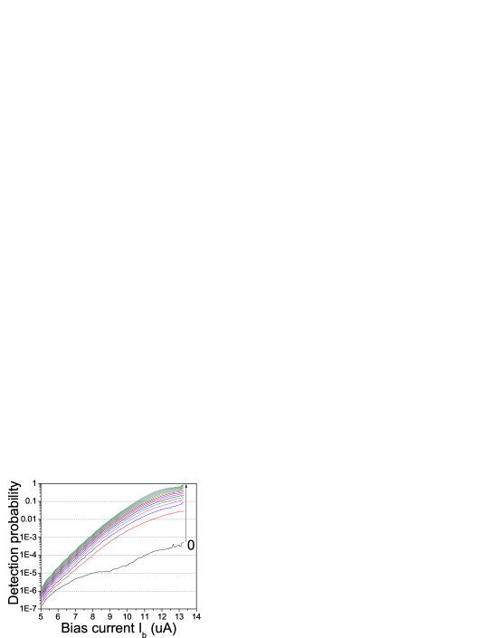
We start by measuring the detector response curves, i.e. the detection probablity versus detector bias current, for a set of coherent states. From these, we deduce the more fundamental response curves for Fock states. Fig. 1 shows the resulting set of inferred detector response curves, i.e. the probability of the detector to respond to a certain Fock state. The detector tomography is performed by a method based on the one described in (Renema et al., 2012). The essential assumption is one of sparsity: we describe the detector by as few physical parameters as possible, while not restricting the possible range of behaviours that our model describes. More specifically, we describe our detector by a combination of linear attenuation (given by linear losses in the detection process such as the finite absorption of the NbN layer) followed by a nonlinear photodetection process inside the NbN layer. The reason for including a linear efficiency seperately is that it significantly reduces the number of parameters required to model the detector, making the tomography more robust.
A second reason is that nonunity linear efficiency introduces correlations between the various at one bias current. The reason for this is that at nonunity efficiency, the photons necessary for an -photon nonlinear process could have come from any number of incident photons. By explicitly including this effect, we make sure that our reconstructed POVM is compatible with this process.
This description in terms of a linear absorber and a nonlinear process, which we showed to be applicable to the NbN nanodetector (Bitauld et al., 2010) is applicable to the SSPD as well. We can therefore write for the click probability:
| (2) |
where is the linear efficiency, is the mean photon number, is the count rate at a given bias current and the are the POVM elements prior to the inclusion of the finite linear efficiency. These elements now only include the nonlinear effects of the detector, i.e. the photon number threshold regime that the detector is in, which depends on the bias current.
After each fit, where the fits at different currents are completely independent, we reinclude the into the to produce the POVM element by the following procedure: first, we fix the number at which we are going to truncate the Hilbert space for the reconstruction. Then, we construct a vector of length , where the first 5 elements are and the other elements are equal to 1. Finally, we multiply this vector by a Bernouilli transformation (Scully1969) , absorbing the linear losses into the POVM. We perform state reconstruction with the POVM consisting of all obtained at different currents.
For this experiment, we are not interested in separating the linear and nonlinear effects, but rather in finding a description of the entire detector. Therefore, we truncate the sum at for all currents. This is equivalent to assuming that the detector is governed only by linear effects at sufficiently high photon numbers. This choice is motivated by the fact that we do not enter the three-photon regime in the current range over which we operate our detector and is justified by the good fits obtained with this model.
For the analysis, we grid our measured count rates by linear interpolation, producing 165 current settings, from 5 A to 13.25 A, which is the current range over which we could measure count rates at enough powers to create a good fit. This is also the current range over which we perform the state reconstruction.
V Quantum state reconstruction
Fig 2. shows a representative sample of the reconstructed coherent and thermal states. We reconstruct a series of coherent and thermal states, using the algorithm given by Eq. (1), iterated times. For the quality of our reconstruction we use the fidelity, defined as , where represents the density matrix of the coherent state corresponding to the average number of photons found in the reconstruction.
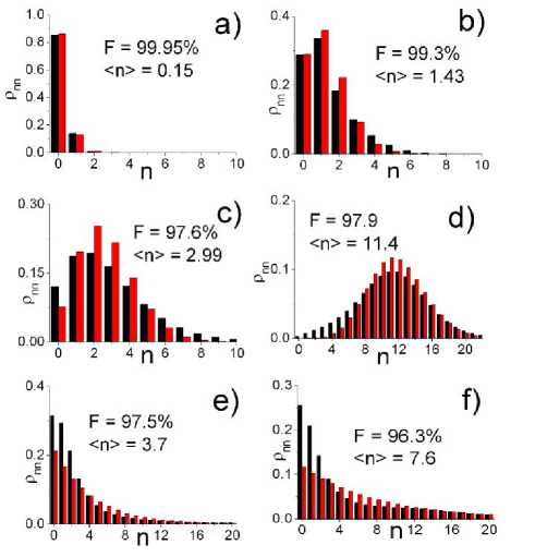
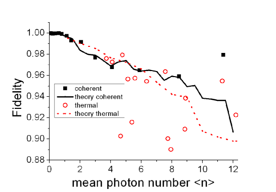
Fig. 3 shows the fidelity of the state reconstruction, as a function of mean photon number. We observe that the quality of the reconstruction degrades as the average number of photons increases. This can be understood from Fig. 1: as the number of photons increases, the curves lie closer together, making it more difficult to distinguish the contributions from various photon numbers.
The theoretical curves in Fig. 3 were generated by simulating the experiment. Each experiment was simulated 30 times, to obtain a reasonable estimate of the expected fidelity. The simulations were performed by calculating expected count rates from the POVM and a given state. For each calculated count rate curve we assumed a constant relative error. We made the approximation that these errors are uniformly distrubuted within the interval .
We compared the mean square error for the reconstructed coherent and thermal states with the theoretically expected count rates for coherent and thermal statistics. From this analysis we conclude that we can successfully distinguish between coherent and thermal states. At larger values of the value of becomes large, indicating that the state reconstruction becomes inaccurate and loses its ability to correctly predict the quantum state. This happens at and for the thermal and coherent states respectively.
By comparison with the measurements, we find that the relative error is 2% for the coherent states, and 6% for the thermal states. These numbers are justified by the observed deviations between count rates expected from the reconstructed states and the measured count rates. We attribute this error to the uncertainty in setting the bias current through the device, where corresponds to 40 nA of uncertainty in the bias current. We attribute the higher uncertainty for the thermal states to residual variations in the input intensity caused by the rotating ground glass plate.
VI Nonlinearity-enhanced QSR
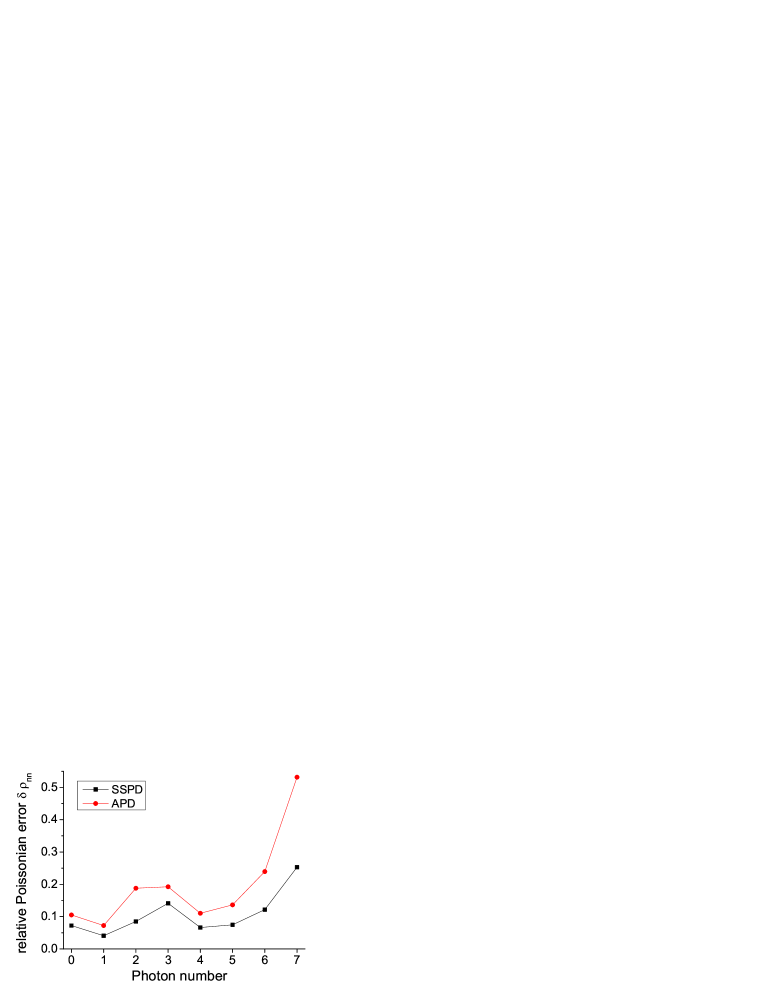
In Fig. 4, we show the effect of the Poissonian (shot-noise) errors on our reconstruction, calculated from the Cramér-Rao bound (Rossi et al., 2004; Zambra et al., 2005). In this figure, we compare the expected error bars for state reconstruction of our SSPD with those of an APD of linear efficiency equal to the SSPD. The shot-noise error is the fundamental lower limit on the error and is fixed for a given state. Therefore, it is relevant to investigate the state reconstruction abilities of a detector.
Fig. 4 shows that the errors in the reconstruction of the SSPD are 50% lower than those of an APD with equivalent efficiency. We attribute this to the nonlinear effects which give our detector higher efficiency at the multiphoton level (Akhlaghi et al., 2012). The physical reason for this nonlinearity is that two photons which are absorbed close together on the nanowire have an enhanced probability to make the detector click. This is in contrast with an avalanche photodiode, where - as long as each photon overcomes the bandgap - there is no mechanism where the photons assist one another in producing an avalanche.
VII Discussion
In previous state reconstruction experiments, avalanche photodiodes (APDs) were used as detectors (Zambra et al., 2005), where the tuning parameter was the attenuation of an extra attenuator inserted in front of the detector. These detectors have a POVM element determined only by linear attenuation, combined with single-photon threshold behaviour. Banaszek has noted before (Banaszek, 1998) that state reconstruction is not limited to containing only linear attenuation. To our knowledge this is the first time that state reconstruction has been performed with a POVM that contains nonlinear as well as linear terms.
We find that the practical limitations of our experiment are the accuracy with which we can set the current. We note, however, that this is no fundamental limitation, as there are current meters available which have a much higher resolution than the one used in our experiment. Furthermore, we note that the Cramer-Rao bound (CRB) has the usual square-root dependence on the number of measurements made, indicating that longer measurement times will improve the quality of the reconstruction as well.
The EM algorithm is known to converge to a solution that saturates the CRB, meaning that we achieve the lowest possible variance (i.e. the optimal solution) for our reconstruction. Moreover, through propagation of errors, the limits on state reconstruction set hard limits on the ability of the detector to measure other quantitites which are functions of the input state, such as the second-order correlation function (van der Vaart, 2000). Therefore, state reconstruction is a fundamental tool to investigate detectors operating at the few-photon level, e.g. multi-element SSPD detectors(Marsili et al., 2009a, b; Jahanmirinejad et al., 2012; Divochiy et al., 2008). Since state reconstruction is performed at the limit of the amount of information that can be extracted from a measurement, investigating the state reconstruction abilities of a detector may yield better understanding of its capabilities. Furthermore, since QSR probes the limits of the abilities of a detector, we propose it as a useful benchmark tool to compare various SSPDs.
In this work, we have used a commercial SSPD, with an efficiency of up to 2.8%. However, recently, great strides have been taken in making SSPDs more efficient, by including cavity structures on the SSPD (Rosfjord et al., 2006; Eduard; Kermanproc), by switching to different materials such as WSi (Marsili93) and by incorporation of SSPDs in nanophotonic waveguides (Goltsmanarxiv; Dondu). Marsili et al report efficiencies as high as 93%. The present work opens up the possibility of using such high-efficiency devices for quantum state reconstruction.
It is an open question whether these more efficient detectors would have beneficial multiphoton nonlinearities similar to the detector reported on in the present work. We note that this nonlinear effect has also been reported in (Akhlaghi et al., 2012), and since it is due to a physical effect that will also be present in more efficient detectors (namely the absorption of two photons close together) there is nothing that precludes it. Detector tomography of a high-efficiency SSPD is necessary to answer this question.
The present work opens up the possibility of applying the ideas of optimal experimental design to the design of SSPDs. For quantum tomography of a spin-1/2 system, there has been work (Nunn et al., 2010) on how to optimize the POVM used in a measurement to yield the optimal tomography result. Similar reasoning may be applied to design an SSPD that is particularly suitable for reconstructing particular states, or for measuring particular properties of states. Such optimization - constrained by what is possible with present production techniques - would focus on the width of the wire (which governs the nonlinearity), length of wire segments, number of elements in a multi-element detector, and the relative size and detection efficiency of each element.
VIII Conclusions
We have shown quantum state reconstruction with an SSPD. The SSPD is especially suited for this task because of its low noise, fast response time, its intrinsic tuning parameter in the form of the bias current through the device, and the nonlinearities which enhances the state reconstruction abilities.
Since the fundamental physics of this device is not known, we have performed a detector tomography procedure in order to find the parameters describing the response of this device (POVM). We thus demonstrate state reconstruction with an experimentally determined POVM. This illustrates the utility of detector tomography.
Acknowledgements.
We thank T. B. Hoang for experimental assistance with the detector. This work is part of the research programme of the Foundation for Fundamental Research on Matter (FOM), which is financially supported by the Netherlands Organisation for Scientific Research (NWO) and was partially funded by the European Commission through FP7 project Q-ESSENCE (Contract No. 248095).References
- Lobino et al. [2008] M. Lobino, D. Korystov, C. Kupchak, E. Figueroa, B. C. Sanders, and A. I. Lvovsky, Science pp. 563–566 (2008).
- Rahimi-Keshari et al. [2011] S. Rahimi-Keshari, A. Scherer, A. Mann, A. T. Rezakhani, A. I. Lvovsky, and B. C. Sanders, New J Phys 13, 013006 (2011).
- Feito et al. [2009] A. Feito, J. S. Lundeen, H. Coldenstrodt-Ronge, J. Eisert, M. B. Plenio, and I. A. Walmsley, New J Phys 11, 093038 (2009).
- Akhlaghi et al. [2012] M. K. Akhlaghi, A. H. Majedi, and J. S. Lundeen, Opt. Express 19 (2012).
- Artiles et al. [2005] L. Artiles, R. Gill, and M. Guta, J. Roy. Stat. Soc. B Met. 67, 109 (2005).
- Banaszek and Wódkiewicz [1996] K. Banaszek and K. Wódkiewicz, Phys. Rev. Lett. 76, 4344 (1996).
- Lundeen et al. [2008] J. S. Lundeen, A. Feito, H. Coldenstrodt-Ronge, K. L. Pregnell, C. Silberhorn, T. C. Ralph, J. Eisert, M. B. Plenio, and I. A. Walmsley, Nat. Phys. 5 (2008).
- Zambra et al. [2005] G. Zambra, A. Andreoni, M. Bondani, M. Gramegna, M. Genovese, G. Brida, A. Rossi, and M. Paris, Phys. Rev. Lett. 95, 063602 (2005).
- Lundeen et al. [2009] J. S. Lundeen, K. L. Pregnell, A. Feito, B. J. Smith, W. Mauerer, C. Silberhorn, J. Eisert, M. B. Plenio, and I. A. Walmsley, J. Mod. Opt. pp. 1–9 (2009).
- Blatt and Wineland [2008] R. Blatt and D. Wineland, Nature 453, 1008 (2008).
- Chuang et al. [1998] I. L. Chuang, N. Gershenfeld, M. G. Kubinec, and D. W. Leung, P. Roy. Soc. A-Math. Phy. 454, 447 (1998).
- Mogilevtsev [1998] D. Mogilevtsev, Opt. Commun. 156 (1998).
- Rossi and Paris [2004] A. R. Rossi and M. G. Paris, Euro. Phys. J. D 32, 223 (2004).
- Rehacek et al. [2003] J. Rehacek, Z. Hradil, O. Haderka, J. Perina, and M. Hamar, Phys. Rev. A 67, 061801 (2003).
- Banaszek [1998] K. Banaszek, Acta Phys. Slovaca 48, 6 (1998).
- Banaszek et al. [1999] K. Banaszek, M. G. A. Paris, and M. F. Sacchi, Phys. Rev. 61, 010304 (1999).
- Rossi et al. [2004] A. Rossi, S. Olivares, and M. Paris, Phys. Rev. A 70, 5 (2004).
- Goltsman et al. [2001] G. N. Goltsman, O. Okunev, G. Chulkova, A. Lipatov, A. Semenov, K. Smirnov, B. Voronov, A. Dzardanov, C. Williams, and R. Sobolewski, Appl. Phys. Lett. 79, 705 (2001).
- Zinoni et al. [2007] C. Zinoni, B. Alloing, L. H. Li, F. Marsili, A. Fiore, L. Lunghi, A. Gerardino, Y. B. Vakhtomin, K. V. Smirnov, and G. N. Goltsman, Appl. Phys. Lett. 91, 031106 (2007).
- Natarajan et al. [2010] C. M. Natarajan, A. Peruzzo, S. Miki, M. Sasaki, Z. Wang, B. Baek, S. Nam, R. H. Hadfield, and J. L. OBrien, Appl. Phys. Lett. 96, 211101 (2010).
- Hadfield et al. [2006] R. H. Hadfield, J. L. Habif, J. Schlafer, R. E. Schwall, and S. W. Nam, Appl. Phys. Lett. 89, 241129 (2006).
- Collins et al. [2007] R. Collins, R. Hadfield, V. Fernandez, S. Nam, and G. Buller, Electron. Lett. 43, 180 (2007).
- Kerman et al. [2006] A. J. Kerman, E. A. Dauler, W. E. Keicher, J. K. W. Yang, K. K. Berggren, G. Goltsman, and B. Voronov, Appl. Phys. Lett. 88, 111116 (2006).
- Verevkin et al. [2004] A. Verevkin, A. Pearlman, W. Slysz, J. Zhang, M. Currier, A. Korneev, G. Chulkova, O. Okunev, P. Kouminov, K. Smirnov, et al., J. Mod. Opt. 51, 1447 (2004).
- Korneev et al. [2004] A. Korneev, P. Kouminov, V. Matvienko, G. Chulkova, K. Smirnov, B. Voronov, G. N. Goltsman, M. Currie, W. Lo, K. Wilsher, et al., Appl. Phys. Lett. 84, 5338 (2004).
- Verevkin et al. [2002] A. Verevkin, J. Zhang, R. Sobolewski, A. Lipatov, O. Okunev, G. Chulkova, A. Korneev, K. Smirnov, G. N. Goltsman, and A. Semenov, Appl. Phys. Lett. 80, 4687 (2002).
- Korneev et al. [2005] A. Korneev, V. Matvienko, O. Minaeva, I. Milnostnaya, I. Rubtsova, G. Chulkova, K. Smirnov, V. Voronov, G. Goltsman, W. Slysz, et al., IEEE T. Appl. Supercon. 101, 49 (2005).
- Divochiy et al. [2008] A. Divochiy, F. Marsili, D. Bitauld, A. Gaggero, R. Leoni, F. Mattioli, A. Korneev, V. Seleznev, N. Kaurova, O. Minaeva, et al., Nat. Phot. 2, 302 (2008).
- Renema et al. [2012] J. J. Renema, G. Frucci, Z. Zhou, F. Mattioli, A. Gaggero, R. Leoni, M. J. A. D. Dood, A. Fiore, and M. P. V. Exter, Opt. Express 20, 2806 (2012).
- Hofherr et al. [2010] M. Hofherr, D. Rall, K. Ilin, M. Siegel, A. Semenov, H.-W. Hübers, and N. a. Gippius, J. Appl. Phys. 108, 014507 (2010).
- Bitauld et al. [2010] D. Bitauld, F. Marsili, A. Gaggero, F. Mattioli, R. Leoni, S. Jahanmiri Nejad, F. Lévy, and A. Fiore, Nano Lett. 10, 2977 (2010).
- Martienssen and Spiller [1964] W. Martienssen and E. Spiller, Am. J. Phys. 32, 919 (1964).
- van der Vaart [2000] A. van der Vaart, Asymptotic Statistics (Cambridge University Press, 2000).
- Marsili et al. [2009a] F. Marsili, D. Bitauld, A. Gaggero, S. Jahanmirinejad, R. Leoni, F. Mattioli, and a. Fiore, New J. Phys. 11, 045022 (2009a), ISSN 1367-2630.
- Marsili et al. [2009b] F. Marsili, D. Bitauld, A. Fiore, A. Gaggero, R. Leoni, F. Mattioli, A. Divochiy, A. Korneev, V. Seleznev, N. Kaurova, et al., J. Mod. Opt. 56, 334 (2009b).
- Jahanmirinejad et al. [2012] S. Jahanmirinejad, G. Frucci, F. Mattioli, D. Sahin, A. Gaggero, R. Leoni, and A. Fiore (2012), eprint ArXiv:1203.5477.
- Rosfjord et al. [2006] K. M. Rosfjord, J. K. W. Yang, E. A. Dauler, A. J. Kerman, V. Anant, B. M. Voronov, G. N. Goltsman, and K. K. Berggren, Opt. Express 14, 527 (2006).
- Verma et al. [2012] V. B. Verma, F. Marsili, B. Baek, A. E. Lita, T. Gerrits, J. A. Stern, R. P. Mirin, and S. W. Nam, CLEO Technical Digest (2012).
- Nunn et al. [2010] J. Nunn, B. J. Smith, G. Puentes, and I. A. Walmsley, Phys. Rev. A 81, 042109 (2010).