Signal Processing and Optimal Resource Allocation for the Interference Channel

1   Introduction

1.1    Resource Allocation in Communication Networks

Resource allocation is a fundamental task in the design and management of communication networks. For example, in a wireless network, we must judiciously allocate transmission power, frequency bands, time slots, and transmission waveforms/codes across multiple interfering links in order to achieve high system performance while ensuring user fairness and quality of service (QoS). The same is true in wired networks such as the Digital Subscriber Lines (DSL).

The importance of resource allocation can be attributed to its key role in mitigating multiuser interference. The latter is the main performance limiting factor for heterogeneous wireless networks where the number of interfering macro/pico/femto base stations (BS) can be very large. In addition, resource allocation provides an efficient utilization of limited resources such as transmission power and communication spectrum. These resources are not only scarce but also expensive. In fact, wireless system operators typically spend billions of dollars to acquire licences to operate certain frequency bands. Moreover, the rising cost of electricity for them to operate the infrastructure has already surpassed the salary cost to employees in some countries. Thus, from the system operator’s perspective, efficient spectrum/power utilization directly leads to high investment return and low operating cost (see e.g., Goldsmith (2005) and Cave et al. (2007)). The transmission power of a mobile terminal is another scarce resource. In this case, careful and efficient power allocation is the key to effectively prolong the battery life of mobile terminals.

Current cellular networks allocate orthogonal resources to users. For example, in a time-division multiplex access (TDMA) or a frequency-division multiplex access (FDMA) network, users in the same cell transmit in different time slots/frequency bands, and users in the neighboring cells transmit using orthogonal frequency channels. Although the interference from neighboring cells is suppressed, the overall spectrum efficiency is reduced, as each BS only utilizes a fraction of the available spectrum. According to a number of recent studies FCC (2002); Sahai et al. (2009) current spectrum allocation strategies are not efficient, as at any given time and location, much of the allocated spectrum appears idle and unused. Moreover, users in cell edges still suffer from significant interference from non-neighboring cells, or pico/femto cells. In addition, for cell edge users the signal power from their own cells are typically quite weak. All of these factors can adversely affect their service quality.

To improve the overall system performance as well as user fairness, future wireless standards 3GPP (2011) advocate the notion of a heterogeneous network, in which low-power BSs and relay nodes are densely deployed to provide coverage for cell edge and indoor users. This new paradigm of network design brings the transmitters and receivers closer to each other, thus is able to provide high link quality with low transmission power (Damnjanovic et al. (2011) and Chandrasekhar Andrews (2008)). Unfortunately, close proximity of many transmitters and receivers also introduces substantial in-network interference, which, if not properly managed, may significantly affect the system performance. Physical layer techniques such as multiple input multiple output (MIMO) antenna arrays and multiple cell coordination will be crucial for effective resource allocation and interference management in heterogeneous networks.

An effective resource allocation scheme should allow not only flexible coordination among BS nodes but also sufficiently distributed implementation. Coordination is very effective for interference mitigation among interfering nodes (e.g., Coordinated Multi-Point (CoMP)), but is also costly in terms of signalling overhead. For example, CoMP requires full BS coordination as well as the sharing of transmit data among all cooperating BSs. In contrast, a distributed resource allocation requires far less signaling overhead and no data sharing, albeit at the cost of a possible performance loss. For in-depth discussions of various design issues in heterogenous networks, we recommend the recent articles and books including Foschini et al. (2006), Gesbert et al. (2007), Gesbert et al. (2010), Sawahashi et al. (2010), Damnjanovic et al. (2011), Martín-Sacristán et al. (2009) and Khan (2009).

In this article, we examine several design and complexity aspects of the optimal physical layer resource allocation problem for a generic interference channel (IC). The latter is a natural model for multi-user communication networks. In particular, we characterize the computational complexity, the convexity as well as the duality of the optimal resource allocation problem. Moreover, we summarize various existing algorithms for resource allocation and discuss their complexity and performance tradeoff. We also mention various open research problems throughout the article.

1.2    Notations

Throughout, we use bold upper case letters to denote matrices, bold lower case letters to denote vectors, and regular lower case letters to denote scalars. For a symmetric (or Hermitian) matrix $\mathbf{X}$, the notation $\mathbf{X}\succeq\mathbf{0}$ (or $\mathbf{X}\succ\mathbf{0}$) signifies $\mathbf{X}$ is positive semi-definite (or definite). Users are denoted by subscripts, while frequency tone indices are denoted by superscripts. Zero mean normalized complex Gaussian distributions are denoted by ${\cal CN}(\mathbf{0},\mathbf{I})$.

1.3    Interference Channels

An interference channel (IC) represents a communication network in which multiple transmitters simultaneously transmit to their intended receivers in a common channel. See Fig. 2 for a graphical illustration of the IC. Due to the shared communication medium, each transmitter generates interference to all the other receivers. The IC model can be used to study many practical communication systems. The simplest example is a wireless ad hoc network in which transmitters and their intended receivers are randomly placed. When all these nodes are equipped with multiple antenna arrays, the channel becomes a MIMO IC. See Fig. 2 for a graphical illustration of a 2-user MIMO IC. If each transmitter and receiver pair communicates over multiple parallel subchannels, the resulting overall channel model becomes a parallel IC. This parallel IC model can be used to describe communication networks employing Orthogonal Frequency Division Multiple Access (OFDMA) where the available spectrum is divided into multiple independent tones/channels. Networks of this kind include the DSL network or the IEEE 802.11x networks.

Another practical network is the multi-cell heterogenous wireless network. In the downlink of such network a set of interfering transmitters (BSs) simultaneously transmit to their respective groups of receivers. This channel is hitherto referred as an interfering broadcast channel (IBC). The uplink of this network can be modeled as an interfering multiple access channel (IMAC). See Fig. 4 and Fig. 4 for graphical illustrations of these two channel models. Note that both IMAC and IBC reduce to an IC when there is only a single user in each cell.

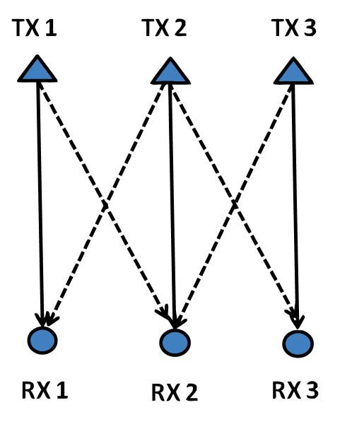
Figure 1: The Interference Channel model. The solid lines represent the direct channels, while the dotted lines represent the interfering channels.

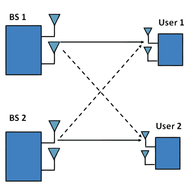
Figure 2: Illustration of a 2-user multiple input multiple output (MIMO) interference channel.

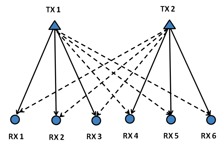
Figure 3: The Interfering Broadcast Channel model. The solid lines represent the direct channels, while the dotted lines represent the interfering channels.

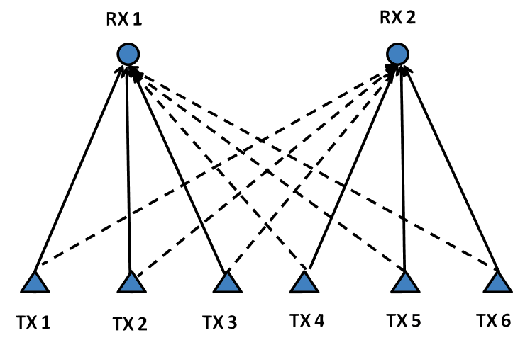
Figure 4: The Interfering Multiple Access Channel model. The solid lines represent the direct channels, while the dotted lines represent the interfering channels.

Our ensuing discussions will be focussed on these channel models. We will illustrate key computational challenges associated with optimal resource allocation and suggest various practical resource allocation approaches to overcome them.

1.4    System Model

We now give mathematical description for three types of IC model – the scalar, parallel and MIMO IC models. Let us assume that there are $K$ transmitter and receive pairs in the system, and we refer to each transceiver pair as a user. Let $\mathcal{K}=\{1,\cdots,K\}$ denote the set of all the users.

1     Scalar IC Model

In a scalar IC model each user transmits and receives a scalar signal. Let $x_{k}\in\mathcal{C}$ denote user $k$’s transmitted signal, and let $p_{k}=|x_{k}|^{2}$ denote its power. Let $\bar{p}_{k}$ denote user $k$’s power constraint: $p_{k}\leq\bar{p}_{k}$. Let $z_{k}\sim\mathcal{CN}(0,1)$ denote user $k$’s normalized complex Gaussian noise with unit variance. Note that we have normalized the power of the noise to unity. Let $H_{lk}\in\mathcal{C}$ denote the channel between transmitter $l$ and receiver $k$. Then user $k$’s received signal $y_{k}\in\mathcal{C}$ can be expressed as

$$y_{k}=\underbrace{H_{kk}x_{k}}_{\textrm{user $k$'s intended signal}}+\underbrace{\sum_{l\neq k}H_{lk}x_{l}}_{\mbox{multiuser interference}}+z_{k}.$$ (1)

The signal to interference plus noise ratio (SINR) for user $k$ is defined as

$$\mbox{SINR}_{k}=\frac{|H_{kk}|^{2}p_{k}}{1+\sum_{l\neq k}|H_{lk}|^{2}p_{l}}.$$ (2)

We denote the collection of all the users’ transmit powers as $\mathbf{p}=\left[p_{1},\cdots,p_{K}\right]^{T}$.

1     Parallel IC Model

In a parallel IC model, the spectrum is divided into $N$ independent non-overlapping bands, each giving rise to a parallel subchannel. Let $\mathcal{N}$ denote the set of all subchannels. Let $x^{n}_{k}\in\mathcal{C}$ denote the transmitted signal of user $k$ on channel $n$, and let $p^{n}_{k}=|x^{n}_{k}|^{2}$ denote its power. We use $\bar{p}_{k}$ to denote user $k$’s power budget so that $\sum_{n=1}^{N}p^{n}_{k}\leq\bar{p}_{k}$. Let $H^{n}_{lk}\in\mathcal{C}$ denote the channel coefficient between the transmitter of user $l$ and the receiver of user $k$ on channel $n$. Let $z^{n}_{k}\sim\mathcal{CN}(0,1)$ denote the Gaussian channel noise. The received signal of user $k$ on subchannel $n$, denoted as $y^{n}_{k}\in\mathcal{C}$, can be expressed as

$$y^{n}_{k}=\underbrace{H^{n}_{kk}x^{n}_{k}}_{\textrm{user $k$'s intended signal}}+\underbrace{\sum_{l\neq k}H^{n}_{lk}x^{n}_{l}}_{\mbox{multiuser interference}}+z^{n}_{k}.$$ (3)

We define the collection of user $k$’s transmit power as $\mathbf{p}_{k}=\left[p^{1}_{k},\cdots,p^{N}_{k}\right]^{T}$, and define all the users’ transmit powers as $\mathbf{p}=\left[\mathbf{p}^{T}_{1},\cdots,\mathbf{p}^{T}_{K}\right]^{T}$.

1     MIMO IC Model

In a MIMO IC model the receivers and transmitters are equipped with $N_{r}$ and $N_{t}$ antennas, respectively. Let $\mathbf{x}_{k}\in\mathcal{C}^{N_{t}}$ and $\mathbf{y}_{k}\in\mathcal{C}^{N_{r}}$ denote the transmitted and received signal of user $k$. Let $\mathbf{H}_{lk}\in\mathcal{C}^{N_{r}\times N_{t}}$ represent the channel gain coefficient matrix between transmitter $l$ and receiver $k$.

Suppose each user $k$ transmits/receives $d_{k}$ data streams, and let $\mathbf{s}_{k}\in\mathcal{C}^{d_{k}\times 1}$ and $\widehat{\mathbf{s}}_{k}\in\mathcal{C}^{d_{k}\times 1}$ denote the transmitted symbols and the received estimated symbols, respectively. Assume that the data vector $\mathbf{s}_{k}$ is normalized so that $\mathbb{E}[\mathbf{s}_{k}\mathbf{s}_{k}^{H}]=\mathbf{I}$, and that the data signals for different users are independent from each other. Throughout this article, we will focus on linear strategies in which users use beamformers to transmit and receive data symbols. Let $\mathbf{V}_{k}\in\mathcal{C}^{N_{t}\times d_{k}}$ and $\mathbf{U}_{k}\in\mathcal{C}^{N_{r}\times d_{k}}$ denote the transmit and receive beamformers, respectively. Let $\mathbf{z}_{k}\sim\mathcal{CN}(0,\mathbf{I}_{N_{r}})$ denote the normalized complex Gaussian noise vector at receiver $k$, where $\mathbf{I}_{N_{r}}$ is the $N_{r}\times N_{r}$ identity matrix. Then the transmitted and received signal for user $k$ can be expressed as

$$\mathbf{x}_{k}=\mathbf{V}_{k}\mathbf{s}_{k}.$$ (4)

$$\mathbf{y}_{k}=\underbrace{\mathbf{H}_{kk}\mathbf{x}_{k}}_{\textrm{user $k$'s intended signal}}+\underbrace{\sum_{l\neq k}\mathbf{H}_{lk}\mathbf{x}_{l}}_{\textrm{multiuser interference}}+{\mathbf{z}_{k}}$$ (5)

$$\widehat{\mathbf{s}}_{k}=\mathbf{U}^{H}_{k}\mathbf{y}_{k}.$$ (6)

Let $\mathbf{Q}_{k}=E[\mathbf{x}_{k}\mathbf{x}_{k}^{H}]$ denote the covariance matrix of the transmitted signal of user $k$. We assume that each transmitter has an averaged total power budget of the form

$$\mbox{Tr}(\mathbf{Q}_{k})\leq\bar{p}_{k},~{}k=1,\cdots,{K}.$$ (7)

When we have a single stream per user, $\mathbf{V}_{k}$ and $\mathbf{U}_{k}$ reduce to vectors $\mathbf{v}_{k}\in\mathcal{C}^{N_{t}\times 1}$ and $\mathbf{u}_{k}\in\mathcal{C}^{N_{r}\times 1}$. In this case the SINR for user $k$’s stream can be defined as

$$\mbox{SINR}_{k}=\frac{|\mathbf{u}^{H}_{k}\mathbf{H}_{kk}\mathbf{v}_{k}|^{2}}{\|\mathbf{u}_{k}\|^{2}+\sum_{l\neq k}|\mathbf{u}^{H}_{k}\mathbf{H}_{lk}\mathbf{v}_{l}|^{2}}.$$ (8)

Multiple Input Single Output (MISO) IC is a special case of MIMO IC in which the receivers only have a single antenna. In this case each user can only transmit a single stream ($d_{k}=1$, $s_{k}\in\mathcal{C}$), and the beamforming matrix $\mathbf{V}_{k}$ reduces to a beamforming vector $\mathbf{v}_{k}\in\mathcal{C}^{N_{t}\times 1}$. The channel coefficient matrix $\mathbf{H}_{kl}$ becomes a row vector $\mathbf{h}_{kl}$, the received signal $\mathbf{y}_{k}$ reduces to a scalar, which can be expressed as

$${y}_{k}=\underbrace{\mathbf{h}_{kk}\mathbf{x}_{k}}_{\textrm{user $k$'s intended signal}}+\underbrace{\sum_{l\neq k}\mathbf{h}_{lk}\mathbf{x}_{l}}_{\textrm{multiuser interference}}+{{z}_{k}}.$$ (9)

The SINR for each user $k$ can be expressed as

$$\mbox{SINR}_{k}=\frac{|\mathbf{h}_{kk}\mathbf{v}_{k}|^{2}}{1+\sum_{l\neq k}|\mathbf{h}_{lk}\mathbf{v}_{l}|^{2}}.$$ (10)

The power budget constraint becomes

$$\|\mathbf{v}_{k}\|^{2}\leq\bar{p}_{k},~{}k=1,\cdots,K.$$ (11)

2   Information-Theoretic Results

2.1    Capacity Results for IC Model

In this subsection we briefly review some information theoretical results related to the capacity of the interference channel.

Consider a single user point to point additive white Gaussian noise (AWGN) scalar channel in the following form

$$y=Hx+z$$ (12)

where $x$, $y$, $H$, $z$ are the transmitted signal, the received signal, the channel coefficient and the Gaussian noise, respectively. Assume that the noise is independently distributed as $z\sim\mathcal{CN}(0,1)$, and that the signal has a power constraint $|x|^{2}\leq\bar{p}$. An achievable transmission rate $R$ for this channel is defined as the rate that can be transmitted and decoded with diminishing error probability. The capacity of a channel $C$ is the supremum of all achievable rates. Let us define the signal to noise ratio (SNR) of the channel as $\mbox{SNR}={\bar{p}|H|^{2}}$, then the capacity of the Gaussian channel is given by

$$C(\mbox{SNR})=\log_{2}\left(1+\mbox{SNR}\right)~{}\textrm{bit per transmission}.$$ (13)

We refer the readers’ to the classic books such as Cover Thomas (2005) and the online course for an introductory treatment of information theory.

Now consider a 2-user interference channel

$$y_{1} = H_{11}x_{1}+H_{21}x_{2}+z_{1}$$

$$y_{2} = H_{22}x_{2}+H_{12}x_{1}+z_{2}.$$ (14)

The capacity region of this channel is the set of all achievable rate pairs of user $1$ and user $2$. Unlike the previous point to point channel, the complete characterization of the capacity region in this simplest 2-user IC case is an open problem in information theory. The largest achievable rate region for the interference channel is the Han-Kobayashi region Han Kobayashi (1981), and it is achieved using superposition coding and interference subtraction. Recently, Etkin et al. (2008) showed that this inner region is within one bit of the capacity region for scalar ICs. The capacity of the scalar interference channel under strong or very strong interference has been found in Carleial (1975), Sato (1981) and Han Kobayashi (1981). In particular, in the very strong interference case, i.e., $\frac{|H_{21}|^{2}}{{|H_{11}|^{2}}}\geq 1+\bar{p}_{1}$ and $\frac{|H_{12}|^{2}}{{|H_{22}|^{2}}}\geq 1+\bar{p}_{2}$, the capacity region is given as

$$R_{k}\leq\log_{2}\left(1+{|H_{kk}|^{2}\bar{p}_{k}}\right),~{}k=1,2$$ (15)

where $R_{k}$ is the transmission rate for user $k$. This result indicates that in very strong interference case the capacity is not reduced. The references Shang et al. (2010) and Chung Cioffi (2007) include recent results that establish the capacity region for more general MIMO and parallel ICs in the strong interference case. However, for the general case where the interference is moderate, the capacity region remains unknown.

The capacity of a communication channel can be approximated by the notion of degrees of freedom. Recall that in the high SNR regime the capacity of a point to point link can be expressed as

$$C(\mbox{SNR})=d\log_{2}(\mbox{SNR})+o(\log_{2}(\mbox{SNR})).$$ (16)

In this case we say the channel has $d$ degrees of freedom. In a 2-user interference channel, the degrees of freedom region can be characterized as follows. Let the sum transmit power across all the transmitters be $\rho$, and let $R_{k}(\rho)$ denote the transmission rate achievable for user $k$. Then the capacity region $C(\rho)$ of this 2-user channel is the set of all achievable rate tuples $(R_{1}(\rho),R_{2}(\rho))$. The degree of freedom region $\mathcal{D}$ for this channel approximates the capacity region, and is defined as (see Cadambe Jafar (2008a))

$$\mathcal{D} = \Bigg{\{}(d_{1},d_{2})\in\mathcal{R}^{2}_{+}:\forall(w_{1},w_{2})\in\mathcal{R}^{2}_{+},w_{1}d_{1}+w_{2}d_{2}$$ (17)

$$\leq \lim_{\rho\to\infty}\sup\left[\sup_{(R_{1}(\rho),R_{2}(\rho))\in C(\rho)}[w_{1}R_{1}(\rho)+w_{2}R_{2}(\rho)]\frac{1}{\log_{2}(\rho)}\right]\Bigg{\}}.$$

The goal of resource allocation is to achieve the optimal performance established by information theory, subject to resource budget constraints. Unfortunately, optimal strategies for achieving the information theoretic limits are often unknown, too difficult to compute or too complicated to implement in practice. For practical considerations, we usually rely on simple transmit/receive strategies (such as linear beamformers) for resource allocation, with the goal of attaining an approximate information theoretic performance bounds. The latter can be in terms of the degrees of freedom or some approximate capacity bounds which we describe next.

2.2    Achievable Rate Regions When Treating Interference as Noise

Due to the difficulties in characterizing the capacity region and the optimal transmit/receive strategy for a general interference channel, many works in the literature study simplified transmit/receive strategies and the corresponding achievable rate regions. One such simplification, which is well motivated from practical considerations, is to assume that low-complexity single user receivers are used and that the multiuser interference is treated as additive noise. The authors of Shang et al. (2009, 2011) show that treating interference as noise in a Gaussian IC actually achieves the sum-rate channel capacity if the channel coefficients and power constraints satisfy certain conditions. These results serve as a theoretical justification for this simplification. In the rest of this article we will treat interference as noise at the receivers. Let us first review some achievable rate region results for different IC models with this simplified assumption.

2     Definition of Rate Region

Consider the 2-user scalar IC (14). The users’ transmission powers are constrained by $0\leq p_{1}\leq\bar{p}_{1}$ and $0\leq p_{2}\leq\bar{p}_{2}$, respectively. The following rates are achievable when the users treat their respective interference as noise

$$R_{1}(p_{1},p_{2}) =\log_{2}\left(1+\mbox{SINR}_{1}\right)$$

$$R_{2}(p_{1},p_{2}) =\log_{2}\left(1+\mbox{SINR}_{2}\right)$$

where the term $\mbox{SINR}_{k}$ has been defined in (2). The directly achievable rate region $\bar{\mathcal{R}}$ is defined as the union of the achievable rate tuples $(R_{1}(p_{1},p_{2}),R_{2}(p_{1},p_{2}))$

$$\bar{\mathcal{R}}=\left\{(R_{1}(p_{1},p_{2}),R_{2}(p_{1},p_{2})):0\leq p_{1}\leq\bar{p}_{1},0\leq p_{2}\leq\bar{p}_{2}\right\}.$$ (18)

The directly achievable rate region represents the set of achievable rates when the transmitters are not able to synchronize with each other (Hui Humblet (1985)). If transmitter synchronization is possible, time-sharing among the extreme points of the directly achievable rate region can be performed. In this case, the achievable rate region becomes the convex hull of the directly achievable rate region (18). Sometimes for convenience, we will refer the directly achievable rate regions simply as rate regions. The exact meaning of the rate region should be clear from the corresponding context.

For a parallel IC model, user $k$’s achievable rate on channel $n$, $R^{n}_{k}$, can be expressed as

$$R^{n}_{k}(p^{n}_{1},\cdots,p^{n}_{K})=\log_{2}\left(1+\frac{|H^{n}_{kk}|^{2}p^{n}_{k}}{1+\sum_{l\neq k}|H^{n}_{lk}|^{2}p^{n}_{l}}\right).$$ (19)

User $k$’s achievable sum rate is the sum of the rates achievable on all the channels

$$R_{k}=\sum_{n=1}^{N}R^{n}_{k}(p^{n}_{1},\cdots,p^{n}_{K}).$$ (20)

The directly achievable rate region $\bar{\mathcal{R}}$ in this case can be expressed as

$$\bar{\mathcal{R}}=\left\{(R_{1},\cdots,R_{K}):\sum_{n=1}^{N}{p^{n}_{k}}\leq\bar{p}_{k},p_{k}\geq 0,\forall~{}k\in\mathcal{K}\right\}.$$ (21)

For a MIMO IC model, user $k$’s achievable rate when treating all other users’ interference as noise is

$$R_{k}(\mathbf{Q}_{1},\cdots,\mathbf{Q}_{K}) =\log_{2}\det\left(\mathbf{I}_{N_{r}}+\mathbf{H}_{kk}\mathbf{Q}_{k}\mathbf{H}_{kk}^{H}\left(\mathbf{I}_{N_{r}}+\sum_{l\neq k}\mathbf{H}_{lk}\mathbf{Q}_{l}\mathbf{H}_{lk}^{H}\right)^{-1}\right).$$ (22)

The directly achievable rate region $\bar{\mathcal{R}}$ can be expressed as

$$\bar{\mathcal{R}}=\left\{(R_{1},\cdots,R_{K}):\mbox{Tr}(\mathbf{Q}_{k})\leq\bar{p}_{k},~{}\mathbf{Q}_{k}\succeq 0,~{}\forall~{}k\in\mathcal{K}\right\}.$$ (23)

2     Characterization of the Directly Achievable Rate Regions

Resource allocation requires a good understanding of the achievable rate regions. The (directly achievable) rate regions of the 2-user and the more general $K$-user scalar IC have been recently characterized in Charafeddine et al. (2007); Charafeddine Paulraj (2009). We briefly elaborate the 2-user rate region and its properties. Let $\Phi(p_{1},p_{2})$ denote a point in the rate region with $x,y$ coordinates representing $R_{1}(p_{1},p_{2})$ and $R_{2}(p_{1},p_{2})$, respectively. Let $\bar{p}_{1}=\bar{p}_{2}=\bar{p}$. Define two functions $\Phi_{1}(p_{2})=\Phi(\bar{p},p_{2})$, and $\Phi_{2}(p_{1})=\Phi(p_{1},\bar{p})$. Then the boundary of the 2-user rate region consists of the union of two axis and the following two curves

$$\Phi_{1}(p_{2}) = \log_{2}\left(1+\frac{\frac{|H_{22}|^{2}}{|H_{21}|^{2}}(|H_{11}|^{2}\bar{p}-(2^{R_{1}}-1))}{(2^{R_{1}}-1)(1+|H_{12}|^{2}\bar{p})}\right),~{}0\leq p_{2}\leq\bar{p}$$ (24)

$$\Phi_{2}(p_{1}) = \log_{2}\left(1+\frac{|H_{22}|^{2}\bar{p}}{1+\frac{|H_{12}|^{2}}{|H_{11}|^{2}}(1+|H_{21}|^{2}\bar{p})(2^{R_{1}}-1)}\right),~{}0\leq p_{1}\leq\bar{p}.$$ (25)

Each of the above two curves consists of the set of rates achievable by one transmitter using its full power, while the other transmitter sweeping over its range of transmit powers. The convexity of this 2-user directly achievable rate region is studied in Charafeddine Paulraj (2009). The following two conditions are sufficient to guarantee the convexity of the directly achievable rate region

$$\frac{\partial^{2}\Phi_{1}(p_{2})}{\partial R^{2}_{1}}\bigg{|}_{p_{2}}<0,~{}\forall~{}0\leq p_{2}\leq\bar{p}$$ (26)

$$\frac{\partial^{2}\Phi_{2}({p}_{1})}{\partial R^{2}_{1}}\bigg{|}_{p_{1}}<0,~{}\forall~{}0\leq p_{1}\leq\bar{p}.$$ (27)

In particular, a necessary condition for (26)-(27) is

$$|H_{22}|^{2}|H_{12}|^{2}\bar{p}(1+|H_{21}|^{2}\bar{p})-|H_{11}|^{2}(1+|H_{22}|\bar{p})<0$$ (28)

which requires that the maximum possible interference to be sufficiently small. As the interference increases, the directly achievable rate regions become non-convex. Fig. 5 shows the transition of the directly achievable rate regions as well as the time-sharing regions when the interference levels change from strong to weak. Clearly, when the interference is strong ($\alpha=2$ in this figure), orthogonal transmission such as TDMA or FDMA is optimal.

Figure 5: The rate regions for a 2-user IC with different interference conditions. $\bar{p}_{1}=\bar{p}_{2}=1$, $|H_{11}|^{2}=|H_{22}|^{2}=1$, $|H_{12}|^{2}=|H_{21}|^{2}=\alpha$. At point $A$ and $C$, a single user transmits using full power. The solid lines are the directly achievable rate frontier. The dotted lines represents the rate boundary that can be achieved by time sharing. Note that the time sharing boundary for $\alpha=0.1$ is the same as the rate region frontier.

The same authors also characterize the achievable rate regions for the general $K$-user case. However the conditions for the convexity of the $K$-user regions are not available and deserve investigation. These conditions can be useful in solving resource allocation problems for an interference network.

More generally, it remains an open problem to derive a complete characterization of the (directly achievable) rate region for a parallel IC. The exact conditions for its convexity (or the lack of) are still unknown, although it is clear that the rate region will be convex if the interference coefficients are sufficiently small.

Several efforts have been devoted to characterizing certain interesting points (such as sum-rate optimal point) on the Pareto boundary of the rate region. Hayashi Luo (2009) have shown that in a parallel IC model with channel gains satisfying the following strong interference conditions

$$\frac{|H^{n}_{lk}|^{2}}{|H^{n}_{kk}|^{2}}>\frac{1}{2},~{}\mbox{and}~{}\frac{|H^{n}_{lk}|^{2}}{|H^{n}_{kk}|^{2}}\frac{|H^{n}_{kl}|^{2}}{|H^{n}_{ll}|^{2}}>\frac{1}{4}\left(1+\frac{1}{C-1}\right)^{2},~{}\forall~{}n\in\mathcal{N},(l,k)\in\mathcal{K}\times\mathcal{K}$$ (29)

where $C\geq 2$ is the minimum number of subchannels used by any user, then the sum rate maximization point can only be achieved using an FDMA strategy. In the special case of 2-user $N$ channel model, the following condition is sufficient for the optimality of FDMA strategy

$$\frac{|H^{n}_{12}|^{2}}{|H^{n}_{22}|^{2}}\frac{|H^{n}_{21}|^{2}}{|H^{n}_{11}|^{2}}>\frac{1}{4}\left(1+\frac{1}{C-1}\right)^{2},~{}\forall~{}n\in\mathcal{N}.$$ (30)

The MIMO IC model is even more general than the parallel IC, hence its achievable rate region is also difficult to characterize. To see this, assuming that $N_{t}=N_{r}=N$; let all the channel matrices be diagonal: $\mathbf{H}_{lk}=\mbox{diag}\left([H^{1}_{lk},\cdots,H^{N}_{lk}]\right)$, $(l,k)\in\mathcal{K}\times\mathcal{K}$; let all the transmission covariances be diagonal as well: $\mathbf{Q}_{k}=\mbox{diag}\left([p^{1}_{k},\cdots,p^{N}_{k}]\right),~{}k\in\mathcal{K}$. In this simplified model, user $k$’s transmission rate reduces to

$$R_{k}(\mathbf{Q}_{1},\cdots,\mathbf{Q}_{K}) = \log_{2}\det\left(\mathbf{H}_{kk}\mathbf{Q}_{k}\mathbf{H}_{kk}^{H}\left(\mathbf{I}_{N_{r}}+\sum_{l\neq k}\mathbf{H}_{lk}\mathbf{Q}_{l}\mathbf{H}_{lk}^{H}\right)^{-1}+\mathbf{I}_{N_{r}}\right)$$ (31)

$$= \sum_{n=1}^{N}\log_{2}\left(1+\frac{p^{n}_{k}|H^{n}_{kk}|^{2}}{1+\sum_{l\neq k}|H^{n}_{lk}|^{2}p^{n}_{l}}\right)$$

which is exactly the rate expression for the $N$ channel $K$ user parallel IC as expressed in (19) and (20).

Larsson Jorswieck (2008) and Jorswieck Larsson (2008) have characterized the achievable rate region of a 2-user MISO IC. In this case, user $k$’s achievable transmission rate reduces to

$$R_{k}(\mathbf{v}_{1},\cdots,\mathbf{v}_{k})=\log_{2}\left(1+\mbox{SINR}_{k}\right)$$ (32)

where the SINR for user $k$ is defined in (10).

Define the maximum-ratio transmission (MRT) and the zero forcing (ZF) beamformers for both users as

$$\begin{array}[]{lll}&\displaystyle\mathbf{v}^{{MRT}}_{1}=\bar{p}_{1}\frac{\mathbf{h}^{H}_{11}}{\|\mathbf{h}^{H}_{11}\|},{}&\displaystyle\mathbf{v}^{{MRT}}_{2}=\bar{p}_{2}\frac{\mathbf{h}^{H}_{22}}{\|\mathbf{h}^{H}_{22}\|}\\[10.0pt] &\displaystyle\mathbf{v}^{{ZF}}_{1}=\bar{p}_{1}\frac{\Pi^{\bot}_{\mathbf{h}^{H}_{12}}\mathbf{h}^{H}_{11}}{\|\Pi^{\bot}_{\mathbf{h}^{H}_{12}}\mathbf{h}^{H}_{11}\|},&\displaystyle\mathbf{v}^{{ZF}}_{2}=\bar{p}_{2}\frac{\Pi^{\bot}_{\mathbf{h}^{H}_{21}}\mathbf{h}^{H}_{22}}{\|\Pi^{\bot}_{\mathbf{h}^{H}_{21}}\mathbf{h}^{H}_{22}\|}\\ \end{array}$$ (33)

where $\Pi^{\bot}_{\mathbf{X}}$ represents the orthogonal projection on to the complement of the column space of $\mathbf{X}$. The authors show that any point on the Pareto boundary is achievable with the beamforming strategy

$$\begin{array}[]{l}\displaystyle\mathbf{v}_{1}(\lambda_{1})=\bar{p}_{1}\frac{\lambda_{1}\mathbf{v}_{1}^{ZF}+(1-\lambda_{1})\mathbf{v}_{1}^{MRT}}{\|\lambda_{1}\mathbf{v}^{ZF}_{1}+(1-\lambda_{1})\mathbf{v}_{1}^{MRT}\|}\\[10.0pt] \displaystyle\mathbf{v}_{2}(\lambda_{2})=\bar{p}_{2}\frac{\lambda_{2}\mathbf{v}_{2}^{ZF}+(1-\lambda_{2})\mathbf{v}_{2}^{MRT}}{\|\lambda_{2}\mathbf{v}^{ZF}_{2}+(1-\lambda_{2})\mathbf{v}_{2}^{MRT}\|}\end{array}$$

where $0\leq\lambda_{1},\lambda_{2}\leq 1$. Intuitively, it is clear that $\mathbf{v}_{1}(\lambda_{1}),\mathbf{v}_{2}(\lambda_{2})$ should stay in the subspace spanned by the channel vectors $\mathbf{h}^{H}_{11},\mathbf{h}^{H}_{22}$. Since this subspace is spanned by the MRT and ZF beamformers, it is no surprise that $\mathbf{v}_{1}(\lambda_{1}),\mathbf{v}_{2}(\lambda_{2})$ can be written as linear combinations of the MRT and ZF beamformers. The novelty of (2.2.2) lies in the claim that the parameters $\lambda_{1},\lambda_{2}$ are real numbers and lie in the interval $[0,1]$. Similar to the characterization (24)-(25) for the rate region of a scalar IC, the characterization (2.2.2) of optimal beamforming strategy can be used to computationally determine the rate region for a 2-user MISO IC.

In Jorswieck et al. (2008), the authors extend their 2-user MISO channel work to a general $K$-user MISO IC. In particular, any point in the achievable rate region can be achieved using a set of beamformers $\{\mathbf{v}_{k}\}_{k=1}^{N}$ that is characterized by $K^{2}$ complex numbers $\{\epsilon_{kl}\}_{(k,l)\in\mathcal{K}\times\mathcal{K}}$ as

$$\begin{array}[]{l}\displaystyle\mathbf{v}_{k}=\sum_{l=1}^{K}\epsilon_{kl}\mathbf{h}^{H}_{kl},~{}\forall~{}k\in\mathcal{K}\\[10.0pt] \displaystyle\|\mathbf{v}_{k}\|^{2}=\bar{p}_{k},~{}\forall~{}k\in\mathcal{K}.\end{array}$$

However, because of the large number of (complex) parameters involved, this characterization appears less useful computationally in the determination of the rate region. We refer the readers to the web pages of Jorswieck and Larsson for more details. We emphasize again that except for these limited results, the structure of a general MIMO IC rate region is still unknown when the interference is treated as noise.

3   Optimal Resource Allocation in Interference Channel

As is evident from the discussions in Section 2, the most interesting points on the boundaries of the rate regions can only be achieved by careful resource allocation. In this section we discuss optimal resource allocation schemes for the general IC models. Such optimality is closely related to the choice of a performance metric for the communication system under consideration.

3.1    Problem Formulations

A communication system should provide users with QoS guarantees, fairness through efficient resource utilization. Mathematically, the resource allocation problem can be formulated as the problem of optimizing a certain system level utility function subject to resource budget constraints.

A popular family of utility functions is the so called “$\alpha$-fair” utility functions, which can be expressed as

$$U\left(\{R_{k}\}_{k=1}^{K}\right)=\sum_{k=1}^{K}\frac{(R_{k})^{1-\alpha}}{1-\alpha}$$ (34)

where $R_{k}$ denotes the transmission rate of user $k$. As pointed out in Mo Walrand (2000), different choices of the parameter $\alpha$ give different priorities to user fairness and overall system performance. We list four commonly used utility functions that belong to the family of $\alpha$-fair utility functions:
a) The sum rate utility: $U_{1}(\{R_{k}\}_{k=1}^{K})=\sum_{k=1}^{K}R_{k}$, obtained by setting $\alpha=0$;
b) The proportional fair utility: $U_{2}(\{R_{k}\}_{k=1}^{K})=\sum_{k=1}^{K}\ln(R_{k})$, obtained by letting $\alpha\to 1$;
c) The harmonic-rate utility: $U_{3}(\{R_{k}\}_{k=1}^{K})=\left(\sum_{k=1}^{K}R^{-1}_{k}\right)^{-1}$, obtained by setting $\alpha=2$;
d) The min-rate utility ($\alpha\to\infty$): $U_{4}(\{R_{k}\}_{k=1}^{K})=\min_{1\leq k\leq K}R_{k}$, obtained by letting $\alpha\to\infty$.
In terms of overall system performance, these utility functions can be ordered as

$$U_{1}\geq U_{2}\geq U_{3}\geq U_{4}.$$ (35)

In terms of user fairness, the order is reversed. We note that except for the case in which the interference is weak, these utility functions are nonconcave in general. For example, in Fig. 6 we plot the sum rate utility for a 2-user scalar IC in cases where the interference is either weak or strong. Moreover, in most cases, it is not possible to represent these utility functions as concave ones via a nonlinear transformation. See Boche et al. (2011) for an impossibility result in scalar interference channel. This is consistent with the complexity status (NP-hard) of the utility maximization problems Luo Zhang (2008); Liu et al. (2011a); Razaviyayn et al. (2011b) (see discussions in Section 3.2).

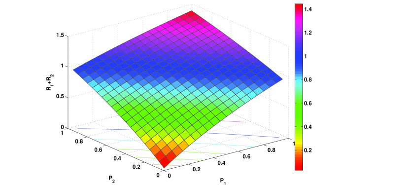
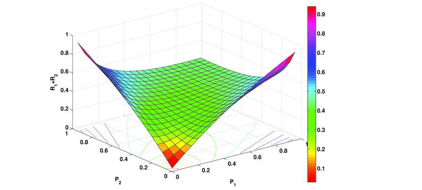
Figure 6: The sum rate utility for a 2-user scalar IC with different interference conditions. $\bar{p}_{1}=\bar{p}_{2}=1$, $|H_{11}|^{2}=|H_{22}|^{2}=1$, $|H_{12}|^{2}=|H_{21}|^{2}=\alpha$. In the left panel, $\alpha=0.5$. In the right panel, $\alpha=5$.

If we wish to find a resource allocation scheme that maximizes the system level performance, then we need to determine the conditions under which the system level problem is easy to solve. Whenever such conditions are met, efficient system level resource allocation decision can be carried out by directly solving a convex optimization problem. Intuitively, when the crosstalk coefficients are zero or sufficiently small (low interference regime), the utility functions should be concave. It will be interesting to analytically determine how small the crosstalk coefficients need to be in order to preserve concavity.

From a practical perspective, the conditions for the concavity of the utility function (in terms of the crosstalk coefficients) are valuable because they can be used to find high quality approximately optimal resource allocation schemes. In particular, we can use these conditions to partition the users into small groups within which the interference is less and resource allocation is easy. Different groups can be put on orthogonal resource dimensions, because the groups cause too much interference to each other. Ultimately a good resource allocation scheme in an interference limited network will likely involve a hybrid scheme whereby some small groups of users share resources, while different groups are separated from competition.

The lack of concavity (or more generally, the lack of concave reformulation/transformation) has made it difficult to numerically maximize these utility functions for resource allocation. To circumvent the computational difficulties, and to reduce the amount of channel state information required for practical implementation, some researchers have proposed to use alternative utility functions for resource allocation. For example, both the mean squared error (MSE) and the leakage power cost functions have been proposed as potential substitutes for the rate-based utility functions listed above Shi et al. (2007) Ulukus Yates (2001) Sadek et al. (2007) and Ho Gesbert (2010). Recently, a number of studies Boche Schubert (2008a); Stanczak et al. (2007); Boche et al. (2011); Boche Schubert (2010) have characterized a family of system utility functions that, under appropriate transformations, admit concave representations. Such transformations allow the associated utility maximization problems to be easily solvable. We refer the readers to Holger Boche’s web page for details on this topic. Unfortunately these utility functions are not directly related to individual users’ transmission rates, hence the solutions of the associated optimization problems tend to give suboptimal system performance (in terms of the users’ achievable rates). We shall not further elaborate on these resource allocation approaches in this article. Instead, we will focus on the use of above listed rate-based utility functions for resource allocation.

Let us describe several utility maximization problems to be considered in this article.

1) Utility maximization for the scalar IC model:

$$\max_{\{p_{k}\}_{k}} U(\{R_{k}\}^{K}_{k=1})$$

s.t. $$R_{k}=\log_{2}\left(1+\frac{|H_{kk}|^{2}p_{k}}{1+\sum_{l\neq k}|H_{lk}|^{2}p_{l}}\right),~{}k=1\cdots,K,$$

$$0\leq{p_{k}}\leq\bar{p}_{k},~{}k=1,\cdots,K.$$

2) Utility maximization for the parallel IC model:

$$\max_{\{p^{n}_{k}\}_{k,n}} U(\{R_{k}\}^{K}_{k=1})$$ (37)

s.t. $$R_{k}=\sum_{n=1}^{N}\log_{2}\left(1+\frac{|H^{n}_{kk}|^{2}p^{n}_{k}}{1+\sum_{l\neq k}|H^{n}_{lk}|^{2}p^{n}_{l}}\right),~{}k=1,\cdots,K,$$

$$\sum_{n=1}^{N}{p^{n}_{k}}\leq\bar{p}_{k},~{}k=1,\cdots,K,$$

$$p^{n}_{k}\geq 0,~{}(k,n)\in\mathcal{K}\times\mathcal{N}.$$

3) Utility maximization for the MISO IC model:

$$\max_{\{\mathbf{v}_{k}\}_{k}} U(\{R_{k}\}^{K}_{k=1})$$ (38)

s.t. $$R_{k}=\log_{2}\left(1+\frac{|\mathbf{h}_{kk}\mathbf{v}_{k}|^{2}}{1+\sum_{l\neq k}|\mathbf{h}_{lk}\mathbf{v}_{l}|^{2}}\right),~{}k=1,\cdots,K,$$

$$\|\mathbf{v}_{k}\|^{2}\leq\bar{p}_{k},~{}k=1,\cdots,K.$$

4) Utility maximization for the MIMO IC model:

$$\max_{\{\mathbf{Q}_{k}\}_{k}} U(\{R_{k}\}^{K}_{k=1})$$ (39)

s.t. $$R_{k}=\log_{2}\det\left(\mathbf{H}_{kk}\mathbf{Q}_{k}\mathbf{H}_{kk}^{H}\left(\mathbf{I}_{N_{r}}+\sum_{l\neq k}\mathbf{H}_{lk}\mathbf{Q}_{l}\mathbf{H}_{lk}^{H}\right)^{-1}+\mathbf{I}_{N_{r}}\right),~{}k=1,\cdots,K$$

$$\mbox{Tr}(\mathbf{Q}_{k})\leq\bar{p}_{k},~{}\mathbf{Q}_{k}\succeq 0,~{}k=1,\cdots,K.$$

5) Utility maximization for the MIMO IC model (single stream per user):

$$\max_{\{(\mathbf{u}_{k},\mathbf{v}_{k})\}_{k=1}^{K}} U(\{R_{k}\}_{k=1}^{K})$$ (40)

s.t. $$R_{k}=\log_{2}\left(1+\frac{|\mathbf{u}^{H}_{k}\mathbf{H}_{kk}\mathbf{v}_{k}|^{2}}{\|\mathbf{u}_{k}\|^{2}+\sum_{l\neq k}|\mathbf{u}^{H}_{k}\mathbf{H}_{lk}\mathbf{v}_{l}|^{2}}\right),~{}k=1,\cdots,K,$$

$$\|\mathbf{v}_{k}\|^{2}\leq\bar{p}_{k},~{}k=1,\cdots,K.$$

A “dual” paradigm for the design of the resource allocation algorithm is to provide QoS guarantees to all the users while minimizing the total power consumption. This formulation traditionally finds its application in voice communication networks where it is desirable to maintain a minimum communication rate (or SINR level) for each user in the system. Define $\{\gamma_{k}\}_{k=1}^{K}$ as the set of SINR targets. We list several QoS constrained min-power problem to be considered in this article.

6) Power minimization for the scalar IC model:

$$\min \sum_{k=1}^{K}p_{k}$$

s.t. $$\mbox{SINR}_{k}\geq\gamma_{k},~{}k=1,\cdots,K,$$

$$\mbox{SINR}_{k}=\frac{|H_{kk}|^{2}p_{k}}{1+\sum_{l\neq k}|H_{lk}|^{2}p_{l}},~{}k=1,\cdots,K.$$

7) Power minimization for the MISO IC model:

$$\min_{\{\mathbf{v}_{k}\}_{k=1}^{K}} \sum_{k=1}^{K}\|\mathbf{v}_{k}\|^{2}$$ (42)

s.t. $$\mbox{SINR}_{k}\geq\gamma_{k},~{}k=1,\cdots,K,$$

$$\mbox{SINR}_{k}=\frac{|\mathbf{h}_{kk}\mathbf{v}_{k}|^{2}}{1+\sum_{l\neq k}|\mathbf{h}_{lk}\mathbf{v}_{l}|^{2}},~{}k=1,\cdots,K.$$

8) Power minimization for the MIMO IC model (single stream per user):

$$\min_{\{(\mathbf{u}_{k},\mathbf{v}_{k})\}_{k=1}^{K}} \sum_{k=1}^{K}\|\mathbf{v}_{k}\|^{2}$$ (43)

s.t. $$\mbox{SINR}_{k}\geq\gamma_{k},~{}k=1,\cdots,K,$$

$$\mbox{SINR}_{k}=\frac{|\mathbf{u}^{H}_{k}\mathbf{H}_{kk}\mathbf{v}_{k}|^{2}}{\|\mathbf{u}_{k}\|^{2}+\sum_{l\neq k}|\mathbf{u}^{H}_{k}\mathbf{H}_{lk}\mathbf{v}_{l}|^{2}},~{}k=1,\cdots,K.$$

A hybrid formulation combines the above two approaches. It aims to provide QoS guarantees while at the same time maximizing a system level utility function. This hybrid formulation is useful in data communication networks where besides the minimum rate constraints, it is preferable to deliver high system throughput. We list two such formulations to be considered later in this article.

9) Hybrid formulation for the scalar IC model:

$$\max U(\{p_{k}\}_{k=1}^{K})$$

s.t. $$\mbox{SINR}_{k}\geq\gamma_{k},~{}k=1,\cdots,K,$$

$$0\leq{p_{k}}\leq\bar{p}_{k},~{}k=1,\cdots,K.$$

10) Hybrid formulation for the parallel IC model:

$$\max_{\{p^{n}_{k}\}_{k,n}} U(\{R_{k}\}^{K}_{k=1})$$ (45)

s.t. $$R_{k}=\sum_{n=1}^{N}\log_{2}\left(1+\frac{|H^{n}_{kk}|^{2}p^{n}_{k}}{1+\sum_{l\neq k}|H^{n}_{lk}|^{2}p^{n}_{l}}\right),~{}k=1,\cdots,K,$$

$$R_{k}\geq\zeta_{k},~{}k=1,\cdots,K,$$

$$\sum_{n=1}^{N}{p^{n}_{k}}\leq\bar{p}_{k},~{}k=1,\cdots,K,$$

$$p^{n}_{k}\geq 0,~{}(k,n)\in\mathcal{K}\times\mathcal{N}$$

where $\{\zeta_{k}\}_{k=1}^{K}$ is a set of rate targets.

We note that for the latter two formulations, the minimum rate/SINR requirements provide fairness to the users, while the optimization objectives are aimed at efficient utilization of system resource (e.g., spectrum or power). For both of these two problems, the feasibility of the set of rate/SINR targets needs to be carefully examined, as the rate/SINR requirements may not be simultaneously satisfiable.

3.2    Complexity of the Optimal Resource Allocation Problems

The aforementioned optimal resource allocation problems are nonconvex. However, the lack of convexity does not necessarily imply that the problem is difficult to solve. In some cases, it may be possible for a nonconvex problem to be appropriately transformed into an equivalent convex one and solved efficiently. A principled approach to characterize the intrinsic difficulty of an utility maximization problem is by way of the computational complexity theory Garey Johnson (1979).

In the following, we summarize a number of recent studies on the computational complexity status of these resource allocation problems. These complexity results suggest that in most cases solving the utility maximization problems to global optimality is computationally intractable as the number of users in the system increases.

Table 1 lists the complexity status for resource allocation problems with specific utility functions for the parallel and MISO IC models. Note that the scalar IC model is included as a special case.

Table 2 summarizes the complexity status for the minimum rate utility maximization problem and the sum power minimization problem with the QoS constraint in MIMO IC model (i.e., problem (40) with min-rate utility and problem (43)). Note that the results in Table 2 are based on the assumption that all transmitters and receivers use linear beamformers and that each mobile receives a single data stream.

Table 1: Complexity status of utility maximization problems for the parallel and MISO IC models (Luo Zhang (2008), Liu et al. (2011a))

	Sum Rate	Proportional Fair	Harmonic Mean	Min-Rate
Parallel IC, $K$=1, $N$ arbitrary	Convex Opt	Convex Opt	Convex Opt	Convex Opt
Parallel IC, $K\geq 2$ fixed, $N$ arbitrary	NP-hard	NP-hard	NP-hard	NP-hard
Parallel IC, $N\geq 2$ fixed, $K$ arbitrary	NP-hard	NP-hard	NP-hard	NP-hard
Parallel IC, $N=1$, $K$ arbitrary	NP-hard	Convex Opt	Convex Opt	LP
MISO IC, $N_{t}\geq 2$, $K$ arbitrary	NP-hard	NP-hard	NP-hard	Poly. Time Solvable

Table 2: Complexity status of the min-rate utility maximization for the MIMO IC model (Liu et al. (2011b)), Razaviyayn et al. (2011b)

	$N_{t}=1$	$N_{t}=2$	$N_{t}\geq 3$
$N_{r}=1$	Poly. Time Solvable	Poly. Time Solvable	Poly. Time Solvable
$N_{r}=2$	Poly. Time Solvable	NP-hard	NP-hard
$N_{r}\geq 3$	Poly. Time Solvable	NP-hard	NP-hard

Recall that the MIMO IC is a generalization of the Parallel IC (see Section 2.2.1). It follows that the complexity results in Table 1 hold true for the MIMO IC model with an arbitrary number of data streams per user. We refer the readers to the author’s web page for recent developments in the complexity analysis as well as other resource allocation algorithms.

3.3    Algorithms for Optimal Resource Allocation

We now describe various utility maximization based algorithms for resource allocation. These algorithms will be grouped and discussed according to their main algorithmic features. Since the min-rate utility function is non-differentiable, it requires a separate treatment that is different from the other utility functions. We begin our discussion with resource allocation algorithms based on the min-rate utility maximization.

3     Algorithms for Min-Rate Maximization

Early works on resource allocation aimed to find optimal transmission powers that can maximize the min-SINR utility. In case of the scalar IC, this problem can be formulated as

$$\max_{\{p_{k}\}_{k\in\mathcal{K}}} \min_{k\in\mathcal{K}}\mbox{SINR}_{k}$$

s.t. $$p_{k}\geq 0,~{}\forall~{}k\in\mathcal{K},$$

$$\mbox{SINR}_{k}~{}\mbox{defined in (\ref{eqSINRScalar})}.$$

In Foschini Miljanic (1993), Zander (1992b) and Zander (1992a), the authors studied the feasibility of this problem and proposed optimal power allocation strategies for it. For randomly generated scalar interference channels, they showed that with probability one, there exists a unique optimum value to the above problem. This optimal value, denoted as $\gamma^{*}$, can be expressed as

$$\gamma^{*}=\frac{1}{\rho(\mathbf{Z})-1}$$ (47)

where $\rho(\mathbf{Z})$ represents the maximum eigenvalue of the matrix $\mathbf{Z}$; $\mathbf{Z}\in\mathcal{R}^{K\times K}$ is a matrix with its $(k,l)^{th}$ element defined as $[\mathbf{Z}]_{k,l}=\frac{|H_{lk}|^{2}}{|H_{kk}|^{2}}$. Distributed power allocation algorithms for this problem were also developed. For example, Foschini Miljanic (1993) proposed an autonomous power control (APC) algorithm that iteratively adjusts the users’ power levels as follows

$$\frac{|H_{kk}|^{2}p^{(t+1)}_{k}}{1+\sum_{l\neq k}|H_{lk}|^{2}p^{(t)}_{l}}=\frac{|H_{kk}|^{2}p^{(t)}_{k}}{1+\sum_{l\neq k}|H_{lk}|^{2}p^{(t)}_{l}}-\beta(\mbox{SINR}^{(t)}_{k}-\gamma^{*})$$ (48)

where $\beta$ is a small positive constant and $t$ is the iteration index. We refer the readers to Hanly Tse (1999) and the web page of Hanly for further discussion of power control techniques for a scalar IC.

For a MISO IC model, the problem of finding optimal transmit beamformers for the maximization of the min-SINR utility has been considered by Bengtsson Ottersten (2001); Wiesel et al. (2006). The corresponding resource allocation problem can be equivalently formulated as

$$\max_{\{\mathbf{v}_{k}\}_{k\in\mathcal{K}}} \gamma$$

s.t. $$\mbox{SINR}_{k}\geq\gamma,~{}k=1,\cdots,K,$$

$$\|\mathbf{v}_{k}\|^{2}\leq\bar{p}_{k},~{}k=1,\cdots,K,$$

$$\mbox{SINR}_{k}~{}\mbox{defined in (\ref{eqMISOSINR})}.$$

This optimization problem (3.3.1) is nonconvex, but can be relaxed to a semidefinite program ( or SDP; see Luo Yu (2006) for an introduction to the related concepts and algorithms). Surprisingly, Bengtsson Ottersten (2001) established that the SDP relaxation for (3.3.1) is tight; see the subsequent section “Algorithms for QoS Constrained Power Minimization” for more discussions. Later, Wiesel et al. (2006) further showed that this nonconvex optimization problem can be solved via a sequence of second order cone programs (SOCP); see Luo Yu (2006) for the definition of SOCP. The key observation is that for a fixed $\gamma$, checking the feasibility of (3.3.1) is an SOCP, which can be solved efficiently by the standard interior point methods. Let $\gamma^{*}$ denote the optimal objective for problem (3.3.1), this max-min SINR problem can be solved by a bisection technique:

1) choose $\epsilon>0$ (termination parameter), $\gamma_{l}$ and $\gamma_{u}$ such that $\gamma^{*}$ lies in $[\gamma_{l},~{}\gamma_{u}]$; 2) let $\gamma_{mid}=(\gamma_{l}+\gamma_{u})/2$; 3) check the feasibility of problem (3.3.1) with $\gamma=\gamma_{mid}$. If feasible, let $\gamma_{l}=\gamma_{mid}$, otherwise set $\gamma_{u}=\gamma_{mid}$. 4) terminate if $\gamma_{u}-\gamma_{l}\leq\epsilon$; else go to step 2) and repeat.

More recently, the max-min fairness resource allocation problem has been considered by Liu et al. (2011b) for the MIMO IC model. Unfortunately, the problem becomes NP-hard in this case (see Table 2).

The joint transceiver beamformer design for the min-SINR maximization problem in a MIMO IC (i.e., problem (40) with min-rate utility) has recently been considered in Liu et al. (2011b) . As shown in Section 3.2, this problem is in general NP-hard. Consequently, they proposed a low-complexity algorithm that converges to a stationary point of this problem. A key observation is that when the receive beamformers $\{\mathbf{u}_{k}\}_{k=1}^{K}$ are fixed, the considered problem can be written as

$$\max_{\{\mathbf{v}_{k}\}_{k=1}^{K}} \gamma$$ (50)

s.t. $$\frac{|\mathbf{u}^{H}_{k}\mathbf{H}_{kk}\mathbf{v}_{k}|^{2}}{\|\mathbf{u}_{k}\|+\sum_{l\neq k}|\mathbf{u}^{H}_{k}\mathbf{H}_{lk}\mathbf{v}_{l}|^{2}}\geq\gamma,~{}k=1,\cdots,K,$$

$$\|\mathbf{v}_{k}\|^{2}\leq\bar{p}_{k},~{}k=1,\cdots,K$$

which has the same form as the MISO min-SINR problem in (3.3.1), and thus can be solved using bisection and SOCP. As a result, the authors propose to alternate between the following two steps to solve the min-rate maximization problem:

1) for fixed $\{\mathbf{u}^{(t)}_{k}\}_{k=1}^{K}$, solve (50) via SOCP to obtain $\{\mathbf{v}^{(t+1)}_{k}\}_{k=1}^{K}$; 2) for fixed $\{\mathbf{v}^{(t+1)}_{k}\}_{k=1}^{K}$, update $\{\mathbf{u}^{(t+1)}_{k}\}_{k=1}^{K}$ to the minimum mean square error (MMSE) receiver:
   $\mathbf{u}_{k}^{(t+1)}=\left(\sum_{l=1}^{K}\mathbf{H}_{lk}\mathbf{v}^{(t+1)}_{l}(\mathbf{H}_{lk}\mathbf{v}_{l}^{(t+1)})^{H}+\mathbf{I}\right)^{-1}\mathbf{H}_{kk}\mathbf{v}^{(t+1)}_{k}$.

Unlike the MISO min-SINR case, only local optimal solutions can be found in the MIMO case. Extending the above algorithm to the MIMO IC/IBC/IMAC case with multiple data streams per user is not a trivial task. For a MIMO IC model, the feasibility problem becomes

$$R_{k}=\log_{2}\det\left(\mathbf{H}_{kk}\mathbf{Q}_{k}\mathbf{H}_{kk}^{H}\left(\mathbf{I}_{N_{r}}+\sum_{l\neq k}\mathbf{H}_{lk}\mathbf{Q}_{l}\mathbf{H}_{lk}^{H}\right)^{-1}+\mathbf{I}_{N_{r}}\right)\geq\zeta,~{}k=1,\cdots,K$$

$$\mbox{Tr}(\mathbf{Q}_{k})\succeq 0,~{}\mbox{Tr}(\mathbf{Q}_{k})\leq\bar{p}_{k},~{}k=1,\cdots,K.$$

This problem is nonconvex and there is no known convex reformulation for it. Finding efficient and preferably distributed algorithms for these channel models is a challenging problem which deserves investigation.

3     Algorithms for Weighted Sum-Utility Maximization

In addition to the min-rate (min-SINR) utility, we can use other utility functions to allocate resources. For instance, let $\{\mu_{k}\}_{k=1}^{K}$ denote a set of positive weights that represent the relative priorities of the users in the system. Then the weighted sum-rate maximization (WSRM) problem for a parallel IC can be formulated as

$$\max_{\{p^{n}_{k}\}_{k,n}} \sum_{k=1}^{K}\mu_{k}R_{k}$$ (51)

s.t. $$R_{k}=\sum_{n=1}^{N}\log_{2}\left(1+\frac{|H^{n}_{kk}|^{2}p^{n}_{k}}{1+\sum_{l\neq k}|H^{n}_{lk}|^{2}p^{n}_{l}}\right),$$

$$\sum_{n=1}^{N}{p^{n}_{k}}\leq\bar{p}_{k},~{}p_{k}\geq 0,~{}k=1,\cdots,K.$$

This simply corresponds to the problem (37) with $\sum_{k=1}^{K}\mu_{k}R_{k}$ as the objective function. WSRM is a central problem for physical layer resource allocation. Many sum-utility maximization problems can be reduced to solving a sequence of WSRM problems for the single channel $N=1$ case, see Luo Zhang (2009). Unfortunately, the complexity results in Section 3.2 indicate that WSRM is in general a hard problem which can not be solved to global optimality by a polynomial time algorithm (unless NP=P). As a result, many works are devoted to finding high quality locally optimal solutions for the WSRM problem.

Algorithms based on Lagrangian dual decomposition

The linear additive structure of the power budget constraints in the weighted sum-utility maximization problem (37) can be exploited by Lagrangian dualization. In particular, Yu Lui (2006) (see also Luo Zhang (2008, 2009)) considered the Lagrangian dual relaxation of the utility maximization problem (37) for the parallel IC model. Let us define the dual function of the primal problem (37) as

$$d({\mbox{\boldmath$\lambda$}})=\max_{\{p^{n}_{k}\geq 0\}_{k,n}}\left\{U(\{R_{k}\}^{K}_{k=1})-\sum_{k=1}^{K}\lambda_{k}\left(\sum_{n=1}^{N}{p^{n}_{k}}-\bar{p}_{k}\right)\right\}$$ (52)

where ${\mbox{\boldmath$\lambda$}}=\{\lambda_{k}\geq 0\}_{k=1}^{K}$ is the set of dual variables associated with the sum power constraints. Then the dual problem of the utility maximization problem can be expressed as follows

$$\min_{{\mbox{\boldmath$\lambda$}}} ~{}d({\mbox{\boldmath$\lambda$}})$$ (53)

s.t. $$\lambda_{k}\geq 0,~{}k=1,\cdots,K.$$

Denote the optimal objective values of the primal problem (37) and the dual problem (53) with $N$ channels as $p^{*}_{N}$ and $d^{*}_{N}$, respectively. By the standard duality theory in optimization Boyd Vandenberghe (2004), we have that the duality gap $d^{*}_{N}-p^{*}_{N}$ satisfies

$$d^{*}_{N}-p^{*}_{N}\geq 0.$$ (54)

When the primal problem is convex, strong duality holds and the inequality becomes equality. When restricted to the FDMA (Frequency Division Multiple Access) solutions, the Lagrangian dual problem decomposes across tones and is efficiently solvable Hayashi Luo (2009) and Luo Zhang (2009). However, when the dual optimal solutions are not unique, it is difficult to construct a primal optimal solution for the problem (37). Luo Zhang (2009) proposed to use an additional randomized step to generate a primal feasible solution from the dual optimal solution.

When the primal problem is not restricted to the FDMA solutions, the Lagrangian dual function is difficult to compute, let alone optimize (see the complexity results in Section 3.2). Yu Lui (2006) proposed an iterative spectrum balancing (ISB) algorithm that alternates between the following two steps to solve the WSRM problem (51):

1) given a ${\mbox{\boldmath$\lambda$}}\geq\mathbf{0}$, use a coordinate ascent strategy to approximately evaluate the dual function until convergence; 2) update $\lambda$ using the subgradient method or the ellipsoid method.

Due to the inexactness of step 1), this algorithm is not guaranteed to converge to a global optimal solution of the WSRM problem (51).

A surprising observation in Yu Lui (2006) is that when $N$ (the number of channels) goes to infinity, the duality gap vanishes. Luo Zhang (2008, 2009) rigorously proved this result using Lyapunov theorem in functional analysis. In particular, Lyapunov’s theorem implies that for the continuous formulation of the WSRM problem (infinite number of channels), the rate region is actually convex. With additional steps to estimate of the approximation of Lebesque integrals, Luo Zhang (2009) showed that for some constant $L$, an estimate of the duality gap is bounded by

$$0\leq d^{*}_{N}-p^{*}_{N}\leq\frac{L}{\sqrt{N}}.$$ (55)

Clearly the gap vanishes as $N$ goes to infinity. Using this estimate, Luo Zhang (2009) further developed a polynomial time approximation scheme to find an optimal FDMA solution for the continuous version of the WSRM problem (51).

Algorithms based on interference pricing

In a number of related works Huang et al. (2006); Yu (2007); Wang et al. (2008); Wu Tsang (2008), the authors proposed a modified iterative water-filling (M-IWF) algorithm that iteratively solves $K$ subproblems. The subproblem related to user $k$ can be expressed as

$$\max_{\{p^{n}_{k}\}_{k,n}} R_{k}-\sum_{n=1}^{N}p^{n}_{k}T^{n}_{k}$$ (56)

s.t. $$\sum_{n=1}^{N}{p^{n}_{k}}\leq\bar{p}_{k},$$

$$p^{n}_{k}\geq 0,~{}n\in\mathcal{N}.$$

where $T^{n}_{k}$ is defined as

$$T^{n}_{k}=\sum_{l\neq k}\left(\frac{|H^{n}_{kl}|^{2}}{\sum_{j\neq k}|H^{n}_{jl}|^{2}p^{n}_{j}+1}-\frac{|H^{n}_{kl}|^{2}}{\sum_{j=1}^{K}|H^{n}_{jl}|^{2}p^{n}_{j}+1}\right).$$ (58)

This term can be viewed as the interference price that user $k$ needs to pay on channel $n$ for the unit of interference it causes to all other users in the system. In other words, the price $T^{n}_{k}$ corresponds to the marginal decrease in the sum-rate utility per unit increase in interference power $p^{n}_{k}$. If the interference price is set to zero, then we are led to the standard iterative water-filling algorithm Yu et al. (2002). The M-IWF algorithm works by iteratively performing the following steps:

1) fix $\left\{T^{n,(t)}_{k}\right\}_{n,k}$, each user iteratively computes the optimal solution $\left\{p^{n,(t+1)}_{k}\right\}_{n,k}$ to the convex subproblem (56) until convergence; 2) update $\left\{T^{n,(t+1)}_{k}\right\}_{n,k}$ according to (58) using $\left\{p^{n,(t+1)}_{k}\right\}_{n,k}$.

We note that the overall computational complexity of step 1) is $O(TKN\log N)$, where $T$ is the total number of iterations needed for convergence. It was conjectured that this algorithm converges at least to a stationary point of the WSRM problem, but no formal proof was given. In Shi et al. (2009a), the authors successfully established the convergence (to the stationary point) of this type of pricing algorithm under the condition that the users act sequentially, i.e., step 1) of M-IWF, only a single user solves its optimization problem (56). They interpreted this sequential M-IWF as a successive linear approximation of the WSRM problem, and showed that the term $-\sum_{n=1}^{N}\sum_{k=1}^{K}p^{n}_{k}T^{n}_{k}$ is the first order Taylor approximation (up to an additive constant term) of $\sum_{l\neq k}R_{l}$, the non-concave part of the objective function. With this interpretation, the M-IWF algorithm can be seen as letting each user sequentially solve a partially linearized version of the WSRM problem. Since the first order Taylor approximation is a locally tight approximation of the weighted sum-rate objective function, the weighted sum-rates computed by the sequential M-IWF algorithm improve monotonically. Moreover, since the users update their power allocations locally, the M-IWF algorithm can be implemented in a distributed manner as long as the interference prices are exchanged among the users at each iteration. We shall refer to the sequential modification of the M-IWF as the multichannel distributed pricing (MDP) algorithm.

The interference pricing idea has been extended to the MISO IC in Shi et al. (2008); Schmidt et al. (2008), and to the MIMO IC with single stream per user in Shi et al. (2009b). The reference Kim Giannakis (2008) considered interference pricing for the general MIMO IC without the single data stream per user restriction. Similar to the parallel IC situation, the convergence of the interference pricing algorithm for the MIMO IC has only been analyzed for the sequential user update case. It will be interesting to see how the pricing technique (and its convergence proof) can be extended to the MIMO IC/IBC/IMAC models with an arbitrary number of streams per user, while allowing simultaneous user updates. A step in this direction was taken by Venturino et al. (2010) which extended the interference pricing technique to the MISO IBC model. Their algorithm (named Iterative Coordinated BeamForming (ICBF)) calculates proper pricing coefficients that enable each BS to update their respective beamformers. Convergence was always observed in the simulation, but no formal proof was given. A recent survey of various pricing techniques used in wireless networks can be found in Schmidt et al. (2009a). We also refer the readers to the web pages of Berry and Honig for other related works on this topic.

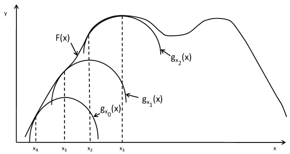
Figure 7: Graphical illustration of the family of algorithms using successive convex approximation. In this example, $x_{0}$ is the initial point. At $x_{0}$, a (strictly) concave function $g_{x_{0}}(x)$ is used to approximate the original non-convex function $F(x)$. The optimal solution of $g_{x_{0}}(x)$, $x_{1}$, is found by standard optimization technique. Then the (strictly) concave function $g_{x_{1}}(x)$ is constructed at the point $x_{1}$. $g_{x_{1}}(x)$ is then optimized to obtain the point $x_{2}$. Continue this process, a stationary solution of the original function $F(x)$ can be found.

Algorithms based on successive convex approximation

The MDP algorithm belongs to a class of algorithms called successive convex approximation (SCA). The idea is to construct and maximize a series of (concave) lower bounds of the original WSRM problem, so that a high quality solution can be obtained asymptotically. See Fig. 7 for a graphical illustration of how this class of algorithms work. In Papandriopoulos Evans (2009), an algorithm called Successive Convex Approximation for Low complExity (SCALE) is proposed to improve the spectral efficiency of the DSL network. This algorithm transforms the noncocave sum rate maximization problem into a series of convex problems by utilizing the following lower bound

$$\alpha\log_{2}(z)+\beta\leq\log_{2}(1+z)$$ (59)

$$\alpha=\frac{z_{0}}{1+z_{0}},~{}\beta=\log_{2}(1+z_{0})-\frac{z_{0}}{1+z_{0}}\log_{2}z_{0}$$ (60)

where the inequality (59) is tight at $z=z_{0}$. This lower bound allows the WSRM problem to be approximated by

$$\max_{\{p^{n}_{k}\}_{k,n}} \sum_{k=1}^{K}\mu_{k}\sum_{n=1}^{N}\alpha^{n}_{k}\log_{2}\left(\frac{|H^{n}_{kk}|^{2}p^{n}_{k}}{1+\sum_{l\neq k}|H^{n}_{lk}|^{2}p^{n}_{l}}\right)+\beta^{n}_{k}$$ (61)

s.t. $$\sum_{n=1}^{N}{p^{n}_{k}}\leq\bar{p}_{k},~{}k=1,\cdots,K$$

$$p^{n}_{k}\geq 0,~{}(k,n)\in\mathcal{K}\times N.$$

After a log transformation $\widetilde{p}^{n}_{k}=\log_{2}(p^{n}_{k}),~{}(k,n)\in\mathcal{K}\times N$, this relaxed problem turns out to be concave in $\widetilde{p}^{k}_{n}$. The SCALE algorithm alternates between the following two steps:

1) fix $\left\{(\alpha^{n,(t)}_{k},\beta^{n,{(t)}}_{k})\right\}_{k,n}$, solve (61) and obtain $\left\{p^{n,(t+1)}_{k}\right\}_{n,k}$; 2) update the parameters $\left\{(\alpha^{n,(t+1)}_{k},\beta^{n,(t+1)}_{k})\right\}_{k,n}$ according to (60) using $\left\{p^{n,(t+1)}_{k}\right\}_{n,k}$.

Step 1) can be solved either in a centralized fashion using Geometric Programming (GP) technique, or by solving the dual problem of (61) in a distributed way. This algorithm is guaranteed to reach a stationary point of the original sum rate maximization problem. We briefly compare the major differences of the MDP and SCALE algorithms in Table 3.

Table 3: Comparison of SCALE and MDP algorithms

	user update schedule	approximation methods	computation per iteration	dual updates
SCALE	simultaneously	concave approximation	iterative	subgradient
MDP	sequentially	linear approximation	closed form	bisection

In Tsiaflakis et al. (2008), a different lower bound is proposed for the WSRM problem. Specifically, the authors decompose the objective function as the difference of two concave functions of $\{p_{k}^{n}\}_{n,k}$ (referred to as the “dc” function)

$$\sum_{k=1}^{K}\sum_{n=1}^{N}\log_{2}\left(1+\frac{|H^{n}_{kk}|^{2}p^{n}_{k}}{1+\sum_{l\neq k}|H^{n}_{lk}|^{2}p^{n}_{l}}\right)$$ (62)

$$= {\sum_{k=1}^{K}\sum_{n=1}^{N}\log_{2}\left(1+\sum_{l\neq k}|H^{n}_{lk}|^{2}p^{n}_{l}+|H^{n}_{kk}|^{2}p^{n}_{k}\right)}-\sum_{k=1}^{K}\sum_{n=1}^{N}\log_{2}\left({1+\sum_{l\neq k}|H^{n}_{lk}|^{2}p^{n}_{l}}\right).$$

Similar to the steps of SCA introduced earlier, in each iteration of the algorithm, the second sum is replaced with its linear lower bound, and the resulting concave maximization problem is solved. Compared to the MDP algorithm which linearizes $\sum_{l\neq k}R_{l}$, this algorithm linearizes all the interference terms in each iteration. As such, it linearizes more terms than the MDP algorithm per iteration.

A related algorithm has been proposed in the recent work Liu et al. (2011a) where the authors considered the general utility maximization problem in MISO IC (i.e., problem formulation (38)). Besides providing complexity results, the authors proposed an algorithm that is able to converge to local optimal solutions for problem (38) with any smooth (twice continuously differentiable) utility functions. The basic idea is to let the users cyclically update their beamformers using projected gradient ascent algorithm. In particular, at iteration $t$, user $k$ takes a gradient projection step to compute the direction $\mathbf{d}_{k}^{(t+1)}$ by solving the following problem

$$\max_{{\mathbf{d}_{k}}} \langle\nabla_{\mathbf{v}_{k}}U(\{\mathbf{v}^{(t)}_{l}\}^{K}_{l=1}),\mathbf{d}_{k}\rangle-\frac{1}{2}\|\mathbf{d}_{k}\|^{2}$$ (63)

s.t. $$\|\mathbf{d}_{k}+\mathbf{v}_{k}^{(t)}\|^{2}\leq\bar{p}_{k},\$$

In contrast to the MDP and SCALE, the subproblem (63) linearizes the entire objective function of (38) at the current point $\{\mathbf{v}_{k}^{(t)}\}_{k\in\mathcal{K}}$, and has an additional quadratic regularization term $\frac{1}{2}\|\mathbf{d}_{k}\|^{2}$. This subproblem is a convex quadratic minimization problem over a ball. As such, it is easier to solve than the corresponding subproblems of MDP and SCALE which are based on partial linearization of the original WSRM objective function. We list below the main steps of this cyclic coordinate ascent (CCA) algorithm:

1) select a user $k\in\mathcal{K}$ and compute its gradient projection direction $\mathbf{d}^{(t+1)}_{k}$ by solving (63); 2) determine stepsize $\alpha^{(t+1)}_{k}$ for user $k$ using a line search strategy; 3) update beamformer: $\mathbf{v}^{(t+1)}_{k}=\mathbf{v}^{(t)}_{k}+\alpha^{(t+1)}_{k}\mathbf{d}^{(t+1)}_{k}$, and go to Step 1).

The CCA algorithm only works in MISO IC case, and it is not clear how to extend it to the MIMO IC.

Algorithms based on weighted MMSE minimization

A different weighted sum-rate maximization approach was proposed in Christensen et al. (2008) for the MIMO broadcast downlink channel, where the WSRM problem is transformed to an equivalent weighted sum MSE minimization (WMMSE) problem with some specially chosen weight matrices. Since the optimal weight matrices are generally unknown, the authors of Christensen et al. (2008) proposed an iterative algorithm that adaptively chooses the weight matrices and updates the linear transmit/receive beamformers at each iteration. A nonconvex cost function was constructed in Christensen et al. (2008) and shown to monotonically decrease as the algorithm progresses. But the convergence of the iterates to a stationary point (or the global minimum) of the cost function is not known. Later, a similar algorithm was proposed in Schmidt et al. (2009b) for the interference channel where each user only transmits one data stream.

It turns out that this WMMSE based resource allocation approach can be extended significantly to handle the MIMO-IC and MIMO-IBC/IMAC models as well as general utility functions. In particular, the authors of Shi et al. (2011a, b) established a general equivalence result between the global (and local) minimizers of the weighted sum-utility maximization problem (e.g., (39) and (51)) and a suitably defined weighed MMSE minimization problem. The latter can be effectively optimized by utilizing the block coordinate descent technique, resulting in independent, closed form iterative update across the transmitters and receivers. The resulting algorithm is named the WMMSE algorithm.

To gain some insight, let us consider the special case of a scalar IC system where the equivalence of the WSRM problem (51) and a weighted sum MSE minimization can be seen more directly. Let $v_{j},\;u_{k}$ denote the complex gains used by the transmitter $j$ and receiver $k$ respectively. Consider the following weighted sum-MSE minimization problem

$$\begin{array}[]{ll}\displaystyle\min_{\{w_{k},u_{k},v_{k}\}_{k=1}^{K}}&\displaystyle\sum_{k=1}^{K}\mu_{k}\left(w_{k}e_{k}-\log w_{k}\right)\\ \textrm{s.t.}&|v_{k}|^{2}\leq{\bar{p}}_{k},~{}k=1,2,\ldots,K\end{array}$$ (64)

where $w_{k}$ is a positive weight variable, and $e_{k}$ is the mean square estimation error

$$e_{k}\triangleq|u_{k}H_{kk}v_{k}-1|^{2}+\sum_{j\neq k}|u_{k}H_{jk}v_{j}|^{2}+|u_{k}|^{2}.$$

To see the equivalence, we can check the first order optimality condition to find the optimal $w_{k}$ and $u_{k}$

$$u_{k}^{opt}=\frac{\overline{H_{kk}v_{k}}}{\sum_{j=1}^{K}|H_{jk}|^{2}|v_{j}|^{2}+1},\quad w_{k}^{opt}=e_{k}^{-1},\quad\forall\ k=1,2,\ldots,K.$$

Plugging these optimal values in (64) gives the following equivalent optimization problem

$$\begin{array}[]{ll}\displaystyle\max_{\{v_{k}\}_{k=1}^{K}}&\displaystyle\sum_{k=1}^{K}\mu_{k}\log\left(1-\frac{|H_{kk}|^{2}|v_{k}|^{2}}{\sum_{j=1}^{K}|H_{jk}|^{2}|v_{j}|^{2}+1}\right)^{-1}\\ \textrm{s.t.}&|v_{k}|^{2}\leq{\bar{p}}_{k},\quad k=1,2,\ldots,K,\end{array}$$

which, upon a change of variable $p_{k}=|v_{k}|^{2}$, is equivalent to

$$\begin{array}[]{ll}\displaystyle\max_{\{p_{k}\}_{k=1}^{K}}&\displaystyle\sum_{k=1}^{K}\mu_{k}\log\left(1+\frac{|H_{kk}|^{2}p_{k}}{\sum_{j\neq k}|H_{jk}|^{2}p_{j}+1}\right)\\ \textrm{s.t.}&p_{k}\leq{\bar{p}}_{k},\quad k=1,2,\ldots,K.\end{array}$$

This establishes the equivalence of the WMMSE problem (64) and the WSRM problem (51). More importantly, the equivalence goes one step further: there is a one-to-one correspondence between the local minimums of the two problems (see Shi et al. (2011a, b)).

The equivalence relation implies that maximizing the weighted sum-rate can be accomplished via iterative weighted MSE minimization. The latter problem is in the space of $(u,v,w)$ and is easier to handle since optimizing each variable while holding the others fixed is convex and easy (e.g., closed form). This property has been exploited in Shi et al. (2011a, b) to design the WMMSE algorithm. In contrast, the original sum-rate maximization problem (51) is in the space of $\mathbf{p}$ and is nonconvex, which makes the iterative optimization process difficult.

The general form of the WMMSE algorithm can handle any utility functions satisfying the following conditions

(Separability) $$U(\{R_{k}\}_{k=1}^{K})=\sum_{k=1}^{K}u_{k}(R_{k})$$ (65)

(Concavity) $$-u_{k}(-\log_{2}\det(\mathbf{X}))~{}~{}\mbox{strictly concave in $\mathbf{X}\succ\mathbf{0}$}~{},\forall~{}k\in\mathcal{K}$$ (66)

(Differentiability) $$u_{k}(x)~{}~{}\mbox{increasing and twice continuously differentiable in $x$}~{},\forall~{}k\in\mathcal{K};$$ (67)

In addition, it also handles a wide range of channel models, e.g., MIMO and parallel IC/IBC/IMAC. It is well known that $R_{k}=\max_{\mathbf{U}_{k}}\log_{2}\det\left(\mathbf{E}_{k}^{-1}(\mathbf{U}_{k},\{\mathbf{V}_{k}\}_{k=1}^{K})\right)$, where $\mathbf{E}_{k}$ is the mean square error (MSE) matrix for user $k$. Define a set of new functions: $c_{k}\left(\mathbf{E}_{k}\right)=-u_{k}\left(-\log\det\left(\mathbf{E}_{k}(\mathbf{U}_{k},\{\mathbf{V}_{k}\}_{k=1}^{K})\right)\right)$, $k=1,\cdots,K$. Similar to the scalar IC case, the equivalence of the following two optimization problems can be established

$$\min_{\{(\mathbf{U}_{k},\mathbf{V})\}_{k=1}^{K}} \sum_{k=1}^{K}c_{k}\left(\mathbf{E}_{k}\right)$$ (68)

s.t. $$\mbox{Tr}(\mathbf{V}_{k}\mathbf{V}^{H}_{k})\leq\bar{p}_{k},~{}k=1,\cdots,K.$$

$$\min_{\{(\mathbf{U}_{k},\mathbf{V}_{k},\mathbf{W}_{k})\}_{k=1}^{K}} \sum_{k=1}^{K}\mbox{Tr}\left(\mathbf{W}^{H}_{k}\mathbf{E}_{k}\right)+c_{k}\left(\phi_{k}(\mathbf{W}_{k})\right)-\mbox{Tr}\left(\mathbf{W}^{H}\phi_{k}(\mathbf{W}_{k})\right)$$ (69)

s.t. $$\mbox{Tr}(\mathbf{V}_{k}\mathbf{V}^{H}_{k})\leq\bar{p}_{k},~{}k=1,\cdots,K.$$

where $\phi_{k}(\mathbf{W}_{k})$ is the inverse map of $\triangledown c_{k}(\mathbf{E}_{k})$. The WMMSE algorithm finds a stationary point of the alternative problem (69). In particular, it alternately updates the three sets of variables $\{\mathbf{U}_{k}\}_{k=1}^{K}$, $\{\mathbf{V}_{k}\}_{k=1}^{K}$ or $\{\mathbf{W}_{k}\}_{k=1}^{K}$ for problem (69), each time keeping two sets of variables fixed. The WMMSE algorithm for a MIMO IC is listed in the following table:

1) Initialize $\{\mathbf{V}_{k}\}_{k\in\mathcal{K}}$ such that $\mbox{Tr}(\mathbf{V}_{k}\mathbf{V}^{H}_{k})={\bar{p}_{k}}$; 2) repeat 3) $\mathbf{W}^{{}^{\prime}}_{k}\leftarrow\mathbf{W}_{k},~{}\forall~{}k\in\mathcal{K}$; 4) $\mathbf{U}_{k}\leftarrow\bigg{(}\sum_{l\in\mathcal{K}}\mathbf{H}_{lk}\mathbf{V}_{l}\mathbf{V}^{H}_{l}\mathbf{H}^{H}_{lk}+\mathbf{I}\bigg{)}^{-1}\mathbf{H}_{kk}\mathbf{V}_{k},~{}\forall~{}k\in\mathcal{K}$; 5) $\mathbf{W}_{k}\leftarrow\left(\mathbf{I}-\mathbf{U}^{H}_{kk}\mathbf{H}_{kk}\mathbf{V}_{k}\right)^{-1},~{}\forall~{}k\in\mathcal{K}$; 6) $\mathbf{V}_{k}\leftarrow\mu_{k}\bigg{(}\sum_{l\in\mathcal{K}}\mu_{l}\mathbf{H}^{H}_{kl}\mathbf{U}_{l}\mathbf{W}_{l}\mathbf{U}^{H}_{l}\mathbf{H}_{kl}+\lambda_{k}^{*}\mathbf{I}\bigg{)}^{-1}\mathbf{H}^{H}_{kk}\mathbf{U}_{k}\mathbf{W}_{k},~{}\forall~{}k\in\mathcal{K}$; 7) until $\left|\sum_{l\in\mathcal{K}}\log\det\left(\mathbf{W}_{l}\right)-\sum_{l\in\mathcal{K}}\log\det\left(\mathbf{W}^{{}^{\prime}}_{l}\right)\right|\leq\epsilon$.

We note that in Step 6), $\lambda_{k}^{*}\geq 0$ is the Lagrangian multiplier for the constraint $\mbox{Tr}(\mathbf{V}_{k}\mathbf{V}^{H}_{k})\leq\bar{P}_{k}$. This multiplier can be found easily by bi-section method. Also, notice that all updates are in closed form (except for $\lambda_{k}^{*}$) and can be performed simultaneously across users.

To compare the performance and the efficiency of various resource allocation methods, we consider a simple simulation experiment involving a parallel-IC and a MIMO-IC. We first specialize the WMMSE algorithm to the parallel-IC scenario and compare it with SCALE and MDP algorithms described earlier. To specialize the WMMSE algorithm for a parallel IC, let us restrict the transmit/receive matrices for each user to be diagonal. That is, the beamforming directions are fixed to be unit vectors and we only optimize power loading factors on the parallel channels. Let $\mathbf{v}_{k}\in\mathcal{C}^{N\times 1}$ denote the user $k$’s transmit filter vector, with ${v}^{n}_{k}$ corresponding to the complex scaling coefficient to be used for the data stream on channel $n$. Similarly, the receive filter vector and the weight vector are denoted by $\mathbf{u}_{k},\mathbf{w}_{k}\in\mathcal{C}^{N\times 1}$ respectively. Then the WMMSE algorithm for the parallel IC channel can be described as

1) Initialize $\{\mathbf{v}_{k}\}_{k\in\mathcal{K}}$ such that $\sum_{n\in\mathcal{N}}{v}^{n}_{k}={\bar{p}_{k}}$; 2) repeat 3) $({w}^{n}_{k})^{{}^{\prime}}\leftarrow{w}^{n}_{k},~{}\forall~{}(n,k)\in\mathcal{N}\times\mathcal{K}$; 4) ${u}^{n}_{k}\leftarrow\bigg{(}\sum_{l\in\mathcal{K}}|{H}^{n}_{lk}|^{2}|{v}^{n}_{l}|^{2}+1\bigg{)}^{-1}{H}^{n}_{kk}{v}^{n}_{k},~{}\forall~{}(n,k)\in\mathcal{N}\times\mathcal{K}$; 5) ${w}^{n}_{k}\leftarrow\bigg{(}1-\overline{u}^{n}_{k}{H}^{n}_{kk}{v}^{n}_{k}\bigg{)}^{-1},~{}\forall~{}(n,k)\in\mathcal{N}\times\mathcal{K}$; 6) ${v}^{n}_{k}\leftarrow\mu_{k}\frac{\overline{H}^{n}_{kk}{u}^{n}_{k}{w}^{n}_{k}}{\sum_{l\in\mathcal{K}}\mu_{l}|{H}^{n}_{kl}|^{2}|{u}^{n}_{l}|^{2}{w}^{n}_{l}+\lambda_{k}^{*}},~{}\forall~{}(n,k)\in\mathcal{N}\times\mathcal{K}$; 7) until $\left|\sum_{l\in\mathcal{K}}\sum_{n\in\mathcal{N}}\log({w}^{n}_{l})-\sum_{l\in\mathcal{K}}\sum_{n\in\mathcal{N}}\log\left(({{w}^{n}}_{l})^{{}^{\prime}}\right)\right|\leq\epsilon$.

In the simulation, we set the weights $\{\mu_{k}\}_{k\in\mathcal{K}}$ all equal to $1$, and set the maximum power $\bar{p}_{k}=10^{\mbox{SNR}/10}$ for all the users. We set the stopping criteria as $\epsilon=0.01$ for all algorithms. The channel coefficients are generated from the complex Gaussian distribution $\mathcal{CN}(0,1)$. For MIMO IC, all the transmitters and receivers are assumed to have the same number of antennas.

We first investigate the performance of SCALE, MDP and the parallel version of the WMMSE algorithm for a parallel IC. Fig. 9 illustrates the sum rate performance of different algorithms when $K=[10,~{}20]$ and $N=32$. We see that these algorithms all have similar performance across all the SNR values. Fig. 9 shows the averaged CPU time comparison of these three algorithms under the same termination criteria and the same accuracy for the search of Lagrangian variables. We observe that the WMMSE requires much less computational time compared to the other two algorithms when the number of users becomes large. Note that the first step in the SCALE algorithm is implemented using the subgradient and the fixed point iterations suggested in (Papandriopoulos Evans, 2009, Section IV-A). The stepsizes for the subgradient method as well as the number of the fixed point iterations need to be tuned appropriately to ensure fast convergence.

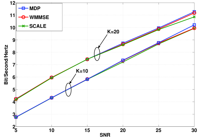
Figure 8: Comparison of the averaged sum rate performance versus SNR of different algorithms in parallel IC. $K=[10,~{}20]$, $N=32$. Each curve in the figure is averaged over 100 random channel realizations.

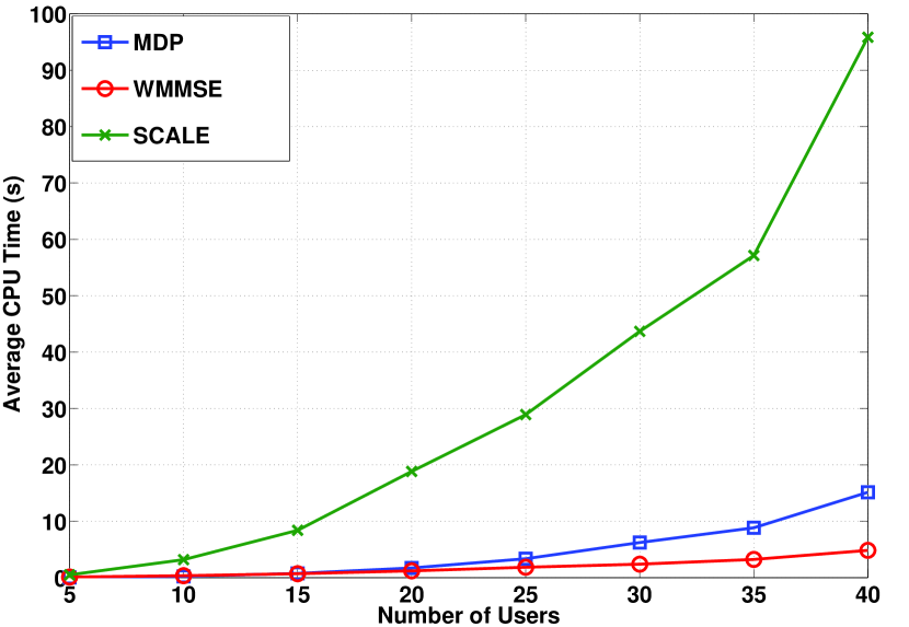
Figure 9: Comparison of the averaged CPU time versus the number of users of different algorithms in parallel IC. $N=32$, $SNR=10$. Each curve in the figure is averaged over 100 random channel realizations.

Next we examine the performance of the WMMSE and the MIMO distributed pricing (MIMO-DP) algorithm developed in Kim Giannakis (2008) in the context of a MIMO-IC. Fig. 11 illustrates the sum rate performance of the two algorithms when $K=[3,~{}10]$ and $N_{r}=N_{t}=3$. Fig. 11 shows the averaged CPU time comparison of the two algorithms. We again observe that the WMMSE requires much less computational time compared with the MIMO-DP algorithm when the number of users becomes large.

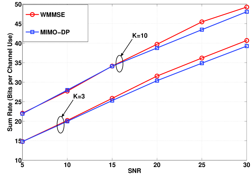
Figure 10: Comparison of the averaged sum rate performance versus SNR of different algorithms in MIMO IC. $K=[3,~{}10]$, $N_{r}=N_{t}=3$. Each curve in the figure is averaged over $100$ random channel realizations

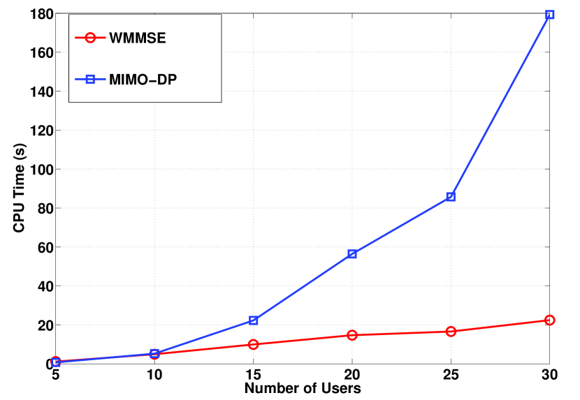
Figure 11: Comparison of the averaged CPU time versus the number of users of different algorithms in MIMO IC. $N_{r}=N_{t}=3$, $\mbox{SNR}=10$. Each curve in the figure is averaged over $100$ random channel realizations

Different from many algorithms discussed earlier (e.g., CCA, MDP), the WMMSE algorithm allows all transmitters/receivers to update their beamformers simultaneously. This feature leads to simple implementation and fast convergence. It will be interesting to see how this algorithm can be further extended to include other utility functions such as the min-rate utility, and to other formulations like QoS constrained power minimization. Also, further research is needed to uncover the full algorithmic potential of WMMSE algorithm for a wide range of applications including joint base station assignment, power control, and beamforming.

Algorithms for cross layer resource allocation

We briefly mention a few cross-layer resource allocation algorithms which require solving a weighted sum-utility problem at each step. These algorithms jointly optimize physical layer as well as the media access (MAC) layer resources to improve the overall system performance.

Recently, Yu et al. (2011) considered the joint MAC layer scheduling and physical layer beamforming and power control in a multicell OFDMA-MIMO network. The algorithm assigns the users to the BSs according to their individual priority and channel status. The beamformers are updated using a MSE duality results developed in Dahrouj Yu (2010) and Song et al. (2007) for multicell network. The transmit powers of the BSs are updated by using the Newton’s method. In Venturino et al. (2009, 2007) and Kim Cho (2009), the authors considered the WSRM problem in a multicell downlink OFDMA wireless network. They proposed to let the BSs alternate between the following two tasks to achieve high system throughput: 1) optimally schedule the users on each channel; 2) jointly optimize their downlink transmit power using a physical layer resource allocation algorithm such as M-IWF or SCALE. Reference Razaviyayn et al. (2009) proposed to adaptively group users into non-interfering groups, and optimize the transceiver structure and the group membership jointly. Such grouping strategy results in fair resource allocation, as cell-edge users with weak channels are protected from the strong users. A generalized version of the WMMSE algorithm has been developed to perform such joint optimization. In all these works the resulting resource allocation schemes achieved a weighted sum-utility that is significantly higher than what is possible with only performing physical layer beamforming/power allocation.

Joint admission control and downlink beamforming is another example of cross layer resource allocation. For a single cell MISO network, this problem has been considered in Matskani et al. (2008, 2009). A related problem is the joint BS selection and power control/beamforming problem. This problem has been addressed in the traditional CDMA based network (see, e.g., Hanly (1995); Yates Huang (1995); Rashid-Farrokhi et al. (1998)), in OFDMA networks (e.g., Hong et al. (2011); Gao et al. (2011); Perlaza et al. (2009)) and in a more general MIMO-HetNet in which all BSs operate on the same frequency bands Hong Luo (2012); Sanjabi et al. (2012). An interesting research direction to pursue is to effectively incorporate these higher layer protocols to boost the system performance for a MIMO and parallel IBC/IMAC network.

3     Algorithms for QoS Constrained Power Minimization

For the scalar IC model, the QoS constrained min-power problem as formulated in (3.1) has been considered in Hanly (1995, 1993) and Yates Huang (1995). They derived conditions for the existence of a feasible power allocation given a set of SINR targets. Define a $K\times K$ matrix $\mathbf{A}$ as follows

$$[\mathbf{A}]_{k,l}=\left\{\begin{array}[]{ll}\frac{\gamma_{k}|H_{lk}|^{2}}{|H_{kk}|^{2}}&\textrm{if }l\neq k\\ 0&\textrm{otherwise }\\ \end{array}\right..$$ (72)

If $\rho(\mathbf{A})<1$, an optimal power allocation $\mathbf{p}=\left[p_{1},\cdots,p_{K}\right]^{T}$ can be found as follows

$$\mathbf{p}=\left(\mathbf{I}_{K}-\mathbf{A}\right)^{-1}\mathbf{b}$$ (73)

where $\mathbf{b}=\left[\frac{\gamma_{1}}{|H_{11}|^{2}},\cdots,\frac{\gamma_{K}}{|H_{KK}|^{2}}\right]^{T}$. The convexity of the feasible SINR region for this problem has been established in Boche Stanczak (2004); Stanczak Boche (2007).

Alternatively, Yates (1995) has provided a framework that allows the users to compute the optimal solution of problem (3.1) distributedly by the following fixed point iteration

$$p^{(t+1)}_{k}=\gamma_{k}\left(\frac{{1+\sum_{l\neq k}|H_{lk}|^{2}p^{(t)}_{l}}}{|H_{kk}|^{2}}\right),k=1,\cdots,K.$$ (74)

This algorithm is shown to have linear rate of convergence, that is,

$$\lim{\sup}_{t\to\infty}\frac{\|\mathbf{p}^{(t+1)}-\mathbf{p}^{*}\|}{\|\mathbf{p}^{(t)}-\mathbf{p}^{*}\|}=c<1$$ (75)

where $\mathbf{p}^{*}$ is the optimal solution of the min-power problem, and $c<1$ is some positive constant. Recently Boche Schubert (2008b) has proposed a different algorithm based on a Newton-type update that exhibits even faster (super-linear) rate of convergence. This algorithm can be applied to more general scenarios when the receivers are equipped with multiple antennas.

When the set of SINR targets cannot be supported by the system (that is, the problem (3.1) is infeasible), the call admission control mechanism should be invoked. A couple of recent works Mitliagkas et al. (2011); Liu et al. (2012) have considered the problem of joint admission and power control arises in the QoS constrained power minimization problem. See Ahmed (2005) for a survey on the general topic of call admission control.

For a MISO IC, Bengtsson Ottersten (1999, 2001) considered the min-power transmit beamforming problem under QoS constraints (problem (42)). Define $\mathbf{V}_{k}=\mathbf{v}_{k}\mathbf{v}^{H}_{k}$ and $\mathbf{G}_{lk}=\mathbf{h}^{H}_{lk}\mathbf{h}_{lk}$, this problem can be equivalently formulated as

$$\min_{\{\mathbf{V}_{k}\}_{k=1}^{K}} \sum_{k=1}^{K}\mbox{Tr}(\mathbf{V}_{k})$$ (76)

s.t. $$\mbox{Tr}(\mathbf{G}_{kk}\mathbf{V}_{k})-\gamma_{k}\sum_{l\neq k}\mbox{Tr}(\mathbf{G}_{lk}\mathbf{V}_{l})=\gamma_{k},~{}k=1,\cdots,K$$

$$\mbox{rank}(\mathbf{V}_{k})=1,\mathbf{V}_{k}\succeq 0,~{}k=1,\cdots,K.$$

Relaxing the rank constraint, this problem is a convex semidefinite program and can be solved efficiently. Interestingly, the authors showed that a rank-one solutions must exist for the relaxed problem, revealing a certain hidden convexity in this problem. The following procedure can be used to construct a rank-1 solution from an optimal solution $\{\mathbf{V}^{*}_{k}\}_{k=1}^{K}$ of the relaxed problem.

1) Take $\mathbf{e}_{k}\in\mbox{span}(\mathbf{V}^{*}_{k})$; 2) Define ${{\mbox{\boldmath$\eta$}}}=[\gamma_{1},\cdots,\gamma_{K}]^{T}$; 3) Define a matrix $\mathbf{F}$ with its elements as $\displaystyle[\mathbf{F}]_{kl}=\left\{\begin{array}[]{ll}-\gamma_{k}\mathbf{e}^{H}_{l}\mathbf{G}_{kk}\mathbf{e}_{l}&\textrm{if }l\neq k,\\ \mathbf{e}^{H}_{k}\mathbf{G}_{kk}\mathbf{e}_{k}&\textrm{otherwise }\\ \end{array}\right.;$ (79) 4) Find $\mathbf{p}=\mathbf{F}^{-1}{{\mbox{\boldmath$\eta$}}}$; 5) Obtain $\mathbf{v}^{*}_{k}=\sqrt{[\mathbf{p}]_{k}}\mathbf{e}_{k}$.

The approach works for the IBC model as well. It can also be extended to include other resource allocation options, such as admission control and base station assignment; see Stridh et al. (2006), Bengtsson (2001) and Rashid-Farrokhi et al. (1998) for details.

3     Algorithms for Hybrid Formulations

For a scalar IC, Chiang et al. (2007) proposed to use a technique called geometric programming (GP) to find an approximate solution to the WSRM problem with QoS constraint. They showed that after approximating the rate function $\log(1+\mbox{SINR}_{k})$ by $\log(\mbox{SINR}_{k})$, the WSRM problem becomes a GP and can be solved efficiently. Moreover, with this approximation, the resource allocation problem falls into the family of problems considered in Boche Schubert (2010); Boche et al. (2011), which can be transformed into equivalent convex optimization problems. For this family of problems, fast and distributed algorithms based on certain Newton-type iteration have been proposed in Wiczanowski et al. (2008).

However, this approximation is not so useful in practice because 1) it is accurate only in high SINR region; 2) it always leads to a solution for which all links are active. The latter feature is undesirable because having all links active can be highly suboptimal when interference is strong. In fact, the main difficulty with WSRM is precisely how to identify which links should be shut off, an important option that is excluded by the GP approximation approach.

Recognizing such problems, the same authors further proposed in Chiang et al. (2007) a successive convex approximation (GP-SCA) method that aims at finding a stationary solution to the original WSRM problem. In particular, let $e_{lk}(\mathbf{p})=|H_{lk}|^{2}p_{l}$, $f_{k}(\mathbf{p})={1+\sum_{l=1}^{K}e_{lk}(\mathbf{p})}$ and $g_{k}(\mathbf{p})={1+\sum_{l\neq k}|H_{lk}|^{2}p_{l}}$, for $k=1,\cdots,K$. Utilizing the arithmetic-geometric mean inequality, the users’ rate functions can be lower-approximate as

$$\log_{2}(1+\mbox{SINR}_{k}) = \log_{2}\left(\frac{f_{k}(\mathbf{p})}{g_{k}(\mathbf{p})}\right)$$ (80)

$$\geq \log_{2}\left(\frac{\prod_{l=1}^{K}\left(\frac{e_{lk}(\mathbf{p})}{\alpha_{l}}\right)^{\alpha_{l}}\times\left(\frac{1}{\beta}\right)^{\beta}}{g_{k}(\mathbf{p})}\right),$$ (81)

$$\mbox{where},~{}~{}\alpha_{l} = \frac{e_{lk}(\widehat{\mathbf{p}})}{f_{k}(\widehat{\mathbf{p}})},~{}\beta=\frac{1}{f_{k}(\widehat{\mathbf{p}})}.$$ (82)

This lower bound is again concave (upon performing a log-transformation), and it is tight when $\mathbf{p}=\widehat{\mathbf{p}}$. The QoS constrained WSRM problem with the approximated objective (81) can be again solved by a GP. A similar alternating procedure as the one we have introduced for the SCALE algorithm can be used to compute a stationary solution to the WSRM problem with QoS constraint.

Algorithms based on global optimization

There are a number of attempts to find globally optimal solution for the WSRM problem. However, these algorithms are all based on implicit enumeration (not surprising in light of the complexity results in Section 3.2). As a result, they can only solve small scale problems and are unlikely to be suitable for implementation in practical applications. However, this does not mean that global optimization algorithms for WSRM are useless. For one thing, they can be a valuable tool to benchmark various low-complexity suboptimal approaches for resource allocation (e.g., those described earlier in this section).

For a scalar IC, Qian et al. (2009) proposed to use an existing algorithm (Frenck Schaible (2006) and Phuong Tuy (2003)) for nonconvex fractional programming to find the global optimal solution for the hybrid problem (3.1). Specifically, introducing a set of auxiliary variable $\{z_{k}\}_{k=1}^{K}$, the scalar WSRM problem with SINR constraint can be formulated into the following equivalent form

$$\max_{\mathbf{z},\mathbf{p}} \prod_{k=1}^{K}(z_{k})^{w_{k}}$$

s.t. $$0\leq{z}_{k}\leq\frac{f_{k}(\mathbf{p})}{g_{k}(\mathbf{p})},$$

$$0\leq p_{k}\leq\bar{p}_{k},~{}\frac{f_{k}(\mathbf{p})}{g_{k}(\mathbf{p})}\geq{\gamma_{k}},\forall~{}k\in\mathcal{K}.$$

This reformulated problem has a concave objective (upon a log transformation), and a nonconvex feasible set $\mathcal{G}$. The global optimization algorithm of Frenck Schaible (2006) and Phuong Tuy (2003) solves the reformulated problem via some convex optimization problems over a sequence shrinking convex sets $S_{1}\supset S_{2}\cdots\supset\mathcal{G}$. The worst case complexity of this algorithm is exponential.

Several other global optimization methods have been proposed to solve the utility maximization problems for more general IC models. For example, Qian Zhang (2009), Xu et al. (2008) and Tan et al. (2009, 2011) considered the parallel IC model, and Jorswieck Larsson (2010) treated the two user-MISO IC model. In particular, the algorithm proposed in Xu et al. (2008) utilized the dc structure (62) of the weighted sum rate function, and applied a branch-and-bound (BB) algorithm to find global optimal solution to the WSRM problem. Due to their exponentially increasing complexity, these algorithms are only suitable for benchmarking resource allocation algorithm for networks with relatively small number of links. For example, the work of Qian Zhang (2009); Qian et al. (2009) compared their global algorithms for a small parallel IC with $N=4$, $K=2$, and a scalar IC with $K$ up to $10$.

An important open problem is how to develop efficient algorithms (suitable for large networks) that can find (provably) tight upper bounds for the system performance.

3     Algorithms for robust resource allocation

All of the aforementioned resource management schemes require perfect channel state information (CSI) at the transmitter side. However, in practice the CSI obtained at the transmitter is susceptible to various sources of uncertainties such as quantization error, channel estimation error or channel aging. These uncertainties may significantly degrade the performance of resource allocation schemes that are designed using perfect CSI. As a result, robust designs are needed for practical resource management.

Several recent contributions considered robust linear transmitter design in a MISO channel with a single transmitter and multiple receivers. Let $\mathbf{h}_{k}\in\mathcal{C}^{N_{t}}$ and $\hat{\mathbf{h}}_{k}\in\mathcal{C}^{N_{t}}$ denote the true channel and the estimated channel between the transmitter and the $k$th receiver, respectively. Let $\mathcal{U}_{k}$ denote the uncertainty set of channel $\mathbf{h}_{k}$, which is the set of possible values that $\mathbf{h}_{k}$ may take after obtaining the estimated channel $\hat{\mathbf{h}}_{k}$. Consider the following specific form of uncertainty set

$$\mathcal{U}_{k}(\mathbf{\Delta}_{k})=\left\{\mathbf{h}_{k}\mid\mathbf{h}_{k}=\hat{\mathbf{h}}_{k}+\mathbf{\Delta}_{k},\|\mathbf{\Delta}_{k}\|\leq\delta_{k}\right\}$$ (84)

where $\mathbf{\Delta}_{k}$ is the vector of estimation error and $\delta_{k}$ is the uncertainty bound. One of the most popular formulation of the robust design is the following QoS constrained min power problem

$$\displaystyle\min_{\{\mathbf{v}_{k}\}_{k=1}^{K}} \quad\sum_{k=1}^{K}\|\mathbf{v}_{k}\|^{2}$$

s.t. $$\quad\frac{|\mathbf{h}_{k}\mathbf{v}_{k}|^{2}}{\sum_{l\neq k}|\mathbf{h}_{k}\mathbf{v}_{l}|^{2}+1}\geq\gamma_{k},~{}\forall~{}\mathbf{h}_{k}\in\mathcal{U}_{k}(\mathbf{\Delta}_{k}),~{}k=1,\cdots,K.$$

This formulation aims at minimizing the total transmission power while ensuring that the SINR constraints are satisfied under all possible channel uncertainties. Define

$$\mathbf{V} =\left[\mathbf{v}_{1},\cdots,\mathbf{v}_{k}\right]$$ (87)

$$\underline{\mathbf{h}}_{k} =\left[\textrm{Re}\{\mathbf{h}_{k}\}\quad\textrm{Im}\{\mathbf{h}_{k}\}\right]$$

$$\underline{\mathbf{V}} =\left[\begin{array}[]{ll}\displaystyle\textrm{Re}\{\mathbf{V}\}&\textrm{Im}\{\mathbf{V}\}\\ \displaystyle-\textrm{Im}\{\mathbf{V}\}&\textrm{Re}\{\mathbf{V}\}\end{array}\right]$$

$$\underline{\mathbf{v}}_{k} =\left[\begin{array}[]{l}\displaystyle\textrm{Re}\{\mathbf{v}_{k}\}\\ \displaystyle-\textrm{Im}\{\mathbf{v}_{k}\}\end{array}\right].$$ (89)

In Shenouda Davidson (2007) problem (3.3.5) has been reformulated into the following semi-infinite SOCP

$$\displaystyle\min_{\underline{\mathbf{V}},t} \quad t$$ (91)

s.t. $$\quad\left\|\textrm{vec}\left(\left[\underline{\mathbf{v}}_{1},\cdots,\underline{\mathbf{v}}_{K}\right]\right)\right\|\leq t$$

$$\quad\left\|\left[\underline{\mathbf{h}}_{k}\underline{\mathbf{V}},~{}1\right]\right\|\leq\sqrt{1+\gamma_{k}^{-1}}\underline{\mathbf{h}}_{k}\underline{\mathbf{v}}_{k},~{}\forall~{}\underline{\mathbf{h}_{k}}\in\mathcal{U}_{k}(\mathbf{\Delta}_{k}),~{}k=1,\cdots,K.$$

This reformulation is a convex restriction to the original problem (3.3.5) in that the the complex magnitude $|\mathbf{h}_{k}\mathbf{v}_{k}|$ in the constraint is replaced by the lower bound equal to its real part $\textrm{Re}(\mathbf{h}_{k}\mathbf{v}_{k})=\underline{\mathbf{h}}_{k}\underline{\mathbf{v}}_{k}$. However, due to the presence of $\underline{\mathbf{h}}_{k}$ on both sides of the SOC constraint (91), this reformulated problem is still difficult to solve. A conservative design is then developed by assuming independent uncertainties for $\underline{\mathbf{h}}_{k}$ on the left and right hand sides of each constraint in (91). With such an assumption, problem (91) can be transformed to the following SDP problem and solved efficiently using standard interior point method.

$$\displaystyle\min_{\underline{\mathbf{V}},{\mbox{\boldmath$\eta$}},{\mbox{\boldmath$\kappa$}},t} \quad t$$ (96)

s.t. $$\quad\left\|\textrm{vec}\left(\left[\underline{\mathbf{v}}_{1},\cdots,\underline{\mathbf{v}}_{K}\right]\right)\right\|\leq t$$

$$\quad\left[\begin{array}[]{lll}\displaystyle\kappa_{k}-\eta_{k}&\mathbf{0}&\left[\underline{\hat{\mathbf{h}}}_{k}\underline{\mathbf{V}},~{}1\right]\\ \displaystyle\mathbf{0}&\eta_{k}\mathbf{I}_{2N_{t}}&\delta_{k}[\underline{\mathbf{V}},\mathbf{0}]\\ \left[\underline{\hat{\mathbf{h}}}_{k}\underline{\mathbf{V}},~{}1\right]^{T}&\delta_{k}[\underline{\mathbf{V}},\mathbf{0}]^{T}&\kappa_{k}\mathbf{I}_{2K+1}\end{array}\right]\succeq 0,~{}k=1,\cdots,K$$

$$\quad\left[\begin{array}[]{ll}\displaystyle\sqrt{1+\gamma_{k}^{-1}}\underline{\hat{\mathbf{h}}}_{k}\underline{\mathbf{v}}_{k}-\kappa_{k}&\delta_{k}\sqrt{1+\gamma_{k}^{-1}}\underline{\mathbf{v}}^{T}_{k}\\ \displaystyle\delta_{k}\sqrt{1+\gamma_{k}^{-1}}\underline{\mathbf{v}}_{k}&\left(\sqrt{1+\gamma_{k}^{-1}}\underline{\hat{\mathbf{h}}}_{k}\underline{\mathbf{v}}_{k}-\kappa_{k}\right)\mathbf{I}_{2N_{t}}\end{array}\right]\succeq 0,~{}k=1,\cdots,K.$$

Instead of solving (91) by the SDP relaxation (96), Vucic Boche (2009) proposed to solve (91) by 1) directly applying the ellipsoid method from convex optimization and 2) approximating (91) by a robust MSE constrained min power problem. Let $u_{k}\in\mathcal{C}$ denote the scalar receive filter used at receiver $k$. Let $\mathbf{e}_{k}$ denote the unit vector with its $k$th element being $1$. Define the MSE of the $k$th user as

$$\textrm{MSE}_{k}\left(\{\mathbf{v}_{k},u_{k}\}_{k=1}^{K}\right)=|u_{k}|^{2}\left(\left(\mathbf{h}_{k}\mathbf{V}-\frac{1}{u_{k}}\mathbf{e}_{k}\right)\left(\mathbf{h}_{k}\mathbf{V}-\frac{1}{u_{k}}\mathbf{e}_{k}\right)^{H}+1\right).$$ (97)

The robust MSE constrained min power problem is given as

$$\displaystyle\min_{\{\mathbf{v}_{k},u_{k}\}_{k=1}^{K}} \quad\sum_{k=1}^{K}\|\mathbf{v}_{k}\|^{2}$$ (98)

s.t. $$\quad\textrm{MSE}_{k}\left(\{\mathbf{v}_{k},u_{k}\}_{k=1}^{K}\right)\leq\frac{1}{1+\gamma_{k}},~{}\forall~{}{\mathbf{h}_{k}}\in\mathcal{U}_{k}(\mathbf{\Delta}_{k}),~{}k=1,\cdots,K.$$ (99)

This problem is convex and can be equivalently formulated as an SDP problem and efficiently solved by interior point methods. It is shown in Vucic Boche (2009) that both the ellipsoid method approach and the robust MSE constrained reformulation approach achieve better performance than the SDP relaxation (96) in terms of various system level performance measures.

As noted earlier, the original min power SINR constrained problem (3.3.5) is not equivalent to the formulation (91), as the latter replaces the nonlinear term $|\mathbf{h}_{k}\mathbf{v}_{k}|$ by a linear lower bound $\textrm{Re}(\mathbf{h}_{k}\mathbf{v}_{k})=\underline{\mathbf{h}}_{k}\underline{\mathbf{v}}_{k}$. Implicit in this reformulation is the additional requirement that $\textrm{Re}(\mathbf{h}_{k}\mathbf{v}_{k})$ is positive for all the channels $\mathbf{h}_{k}\in\mathcal{U}_{k}(\delta_{k})$. Recently, the authors of Song et al. (2011) showed that the direct SDP relaxation of the original problem (3.3.5) is actually tight as long as the size of the uncertainty set is sufficiently small. This implies that robust resource allocation for MISO channels can be solved to global optimality in polynomial time, provided the channel uncertainty is small. More precisely, define $\mathbf{V}_{k}=\mathbf{v}_{k}\mathbf{v}^{H}_{k}$, and $\mathbf{X}_{k}=\frac{1}{\gamma_{k}}\mathbf{V}_{k}-\sum_{l\neq k}\mathbf{V}_{l}$, the problem (3.3.5) can be equivalently reformulated as

$$\displaystyle\min_{\{\mathbf{V}_{k},\kappa_{k}\}_{k=1}^{K}} \quad\sum_{k=1}^{K}\textrm{Tr}(\mathbf{V}_{k})$$

s.t. $$\quad\kappa_{k}\geq 0,~{}k=1,\cdots,K$$

$$\quad\left[\begin{array}[]{ll}\displaystyle\mathbf{X}_{k}+\kappa_{k}\mathbf{I}&\mathbf{X}_{k}\hat{\mathbf{h}}^{H}_{k}\\ \displaystyle\hat{\mathbf{h}}_{k}\mathbf{X}^{H}_{k}&\hat{\mathbf{h}}_{k}\mathbf{X}^{H}_{k}\hat{\mathbf{h}_{k}}^{H}-1-\kappa_{k}\delta_{k}^{2}\end{array}\right]\succeq 0,~{}k=1,\cdots,K.$$

$$\mathbf{V}_{k}\succeq 0,\quad\textrm{rank}(\mathbf{V}_{k})=1,~{}k=1,\cdots,K.$$

When the rank constraints are dropped, this problem becomes the following SDP and can be efficiently solved.

$$\begin{array}[]{lll}\displaystyle&\displaystyle\min_{\{\mathbf{V}_{k},\kappa_{k}\}_{k=1}^{K}}&\quad\sum_{k=1}^{K}\textrm{Tr}(\mathbf{V}_{k})\\ \displaystyle&\ \ \ \textrm{s.t.}&\quad\kappa_{k}\geq 0,~{}k=1,\cdots,K\\ \displaystyle&&\quad\left[\begin{array}[]{ll}\displaystyle\mathbf{X}_{k}+\kappa_{k}\mathbf{I}&\mathbf{X}_{k}\hat{\mathbf{h}}^{H}_{k}\\ \displaystyle\hat{\mathbf{h}}_{k}\mathbf{X}^{H}_{k}&\hat{\mathbf{h}}_{k}\mathbf{X}^{H}_{k}\hat{\mathbf{h}_{k}}^{H}-1-\kappa_{k}\delta_{k}^{2}\end{array}\right]\succeq 0,~{}k=1,\cdots,K.\\ \displaystyle&&\mathbf{V}_{k}\succeq 0,~{}k=1,\cdots,K.\end{array}$$

Let ${\mbox{\boldmath$\delta$}}=[\delta_{1},\cdots,\delta_{K}]$. Let $P_{{\mbox{\boldmath$\delta$}}}$ denote the above SDP problem when the bounds on the uncertainty set is $\delta$. Let $P^{*}({{\mbox{\boldmath$\delta$}}})$ denote the optimal value of the the problem $P_{{\mbox{\boldmath$\delta$}}}$. Suppose that for some choice of uncertainty bounds $\bar{{\mbox{\boldmath$\delta$}}}=\left[\bar{\delta}_{1},\cdots,\bar{\delta}_{K}\right]^{T}>0$, the problem $P_{\bar{{\mbox{\boldmath$\delta$}}}}$ is strictly feasible. Define the set

$$\Omega(\bar{{\mbox{\boldmath$\delta$}}})=\left\{{\mbox{\boldmath$\delta$}}\ \big{|}\ \delta_{k}\leq\bar{\delta}_{k}~{}\textrm{and}~{}\delta_{k}<\sqrt{\frac{\gamma_{k}}{P^{*}\left(\bar{{\mbox{\boldmath$\delta$}}}\right)}},~{}k=1,\cdots,K\right\}.$$ (103)

Then, according to Song et al. (2011), for any vector of uncertainty bounds ${\mbox{\boldmath$\delta$}}\in\Omega(\bar{{\mbox{\boldmath$\delta$}}})$, the problem $P_{{\mbox{\boldmath$\delta$}}}$ is feasible. Moreover, its optimal solution $\{\mathbf{V}^{*}_{k}\}_{k=1}^{K}$ satisfies $\textrm{rank}(\mathbf{V}^{*}_{k})=1,~{}k=1\cdots,K$, and it must be the optimal solution of the original problem (3.3.5).

Alternative system level objectives and constraints can be considered to result in different formulations of the robust resource allocation problem. For example, reference Shenouda Davidson (2008) considered robust design for both the averaged sum MSE minimization problem and the worst case sum MSE minimization problem. Reference Tajer et al. (2011) considered the worst case weighted sum rate maximization problem and min-rate maximization problem. The authors of Zheng et al. (2008) considered the robust beamformer design in a cognitive radio network in which there are additional requirements that the transmitter’s interference to the primary users should be kept under a prescribed level. However, most of the above cited works focus on robust design in a single cell network with a single transmitter. The extensions to the general MIMO IC/IBC/IMAC will be interesting.

Table 4: Comparisons of resource allocation algorithms

Algorithm	Optimality	Complexity	Convergence	Coordination	Message	Channel	Update	Problem
		Per Iteration	Status	Level	Exchange	Model	Schedule	Formulation
APC	Global	$O(K)$	Yes	Distributed	$O(K)$	Scalar IC	Sequential	Min SINR
(Foschini Miljanic (1993))
BB	Global	Lower Bounded By	Yes	Centralized	$N/A$	Parallel IC	N/A	Sum Rate
(Xu et al. (2008))		$O\left((3+B/2)K^{3}+3K^{2}/2+C\right)$
Bisection-SOCP	Global	$O\left(K^{3.5}N_{t}^{3.5}\log(\frac{1}{\epsilon})\right)$	Yes	Centralized	N/A	MISO IC	N/A	Min SINR
(Liu et al. (2011a))
CCA	Local	$O(N_{t}K^{2})$	Yes	Distributed	$O(K^{2})$	MISO IC	Sequential	Smooth
(Liu et al. (2011a))								Utility
ICBF	Unknown	$O(TK^{2}N^{3}_{t})$	Unknown	Distributed	$O(K^{2})$	MISO IC	Sequential	Sum Rate
(Venturino et al. (2010))						MISO IBC/IMAC
ISB	Unknown	$O(BNK)$	Unknown	Distributed	$O(K^{2}N)$	Parallel IC	Sequential	Sum Rate
(Yu Lui (2006))
GP	Unknown	$O(K^{3})$	Yes	Centralized	N/A	Parallel IC	N/A	Mixed
(Chiang et al. (2007))		(Scalar IC Case)				Scalar IC		Sum Rate
NFP	Global	Upper Bounded By	Yes	Centralized	N/A	Parallel IC	N/A	Mixed
(Phuong Tuy (2003))		$K^{t}$				Scalar IC		Sum Rate
MDP	Local	$O(KN\log N+K^{2}N)$	Yes	Distributed	$O(K^{2}N)$	MISO IC	Sequential	Sum Rate
(Shi et al. (2009a))		(Parallel IC Case)				Parallel IC
MIMO-DP	Unknown	$O\left(K^{3}(N_{t}N^{2}_{r}+N^{2}_{t}N_{r})+K^{2}N^{3}_{r}\right)$	Unknown	Distributed	$O(K^{2}N^{2}_{r})$	MIMO IC	Sequential	Sum Rate
(Kim Giannakis (2008))
M-IWF	Unknown	$O(TKN\log N+K^{2}N)$	Unknown	Distributed	$O(K^{2}N)$	Parallel IC	Simultaneous	Sum Rate
(Yu (2007))
SCALE-Dual	Local	$O(TKN+NK^{2})$	Yes	Distributed	$O(K^{2}N)$	Parallel IC	Simultaneous	Sum Rate &
(Papandriopoulos Evans (2009))								Min Power
SCALE-GP	Local	$O\left(K^{4}N^{4}\log(KN/\epsilon)\right)$	Yes	Centralized	N/A	Parallel IC	N/A	Sum Rate &
(Papandriopoulos Evans (2009))								Min Power
WMMSE-MIMO	Local	$O\left(K^{2}(N_{t}N^{2}_{r}+N^{2}_{t}N_{r}+N^{3}_{t})+KN^{3}_{r}\right)$	Yes	Distributed	$O(K^{2}N^{2}_{r})$	MIMO IC	Simultaneous	Utility Satisfy
(Shi et al. (2011b))		(MIMO IC Case)				MIMO IBC/IMAC		(65)-(67)
WMMSE-Parallel	Local	$O\left(K^{2}N^{3}\right)$	Yes	Distributed	$O(K^{2}N^{2})$	Parallel IC	Simultaneous	Utility Satisfy
(Shi et al. (2011b))		(MIMO IC Case)				Parallel IBC/IMAC		(65)-(67)

To close this section, we summarize the properties of most of the algorithms discussed in this section in Table 4. These algorithms usually admit certain forms of decentralized implementation, in which the computational loads are distributed to different entities in the network. We emphasize that the per-iteration computational complexity and the amount of message exchanges are important characteristics for practical implementation of these distributed algorithms. Efficient computation ensures real time implementation, while fewer number of message exchanges per iteration implies less signaling overhead. In Table 4, these characteristics are listed for each of the algorithms. We note that the computational complexity and the required message exchanges are calculated on a per iteration basis, where in one iteration each user $k\in\mathcal{K}$ completes one update. Also note that in Table 4, the variable $T$ in ICBF, SCALE-Dual and M-IWF represents the number of inner iterations needed; the variable $\epsilon$ in Bisection-SOCP and SCALE-GP represents the required precision for their respective inner solutions; the variable $t$ in MAPEL represents the iteration index; the variable $B$ in BB and ISB represents the maximum number of transmitted bits allowed for each subchannel; the variable $C$ in the BB algorithm represents its computation overhead.

4   Distributed Resource Allocation in Interference Channel

Most of the algorithms introduced in the previous section are either centralized or require certain level of user coordination. Such coordination may be costly in infrastructure based networks, and is often infeasible for fully distributed networks. In this section we discuss fully distributed resource allocation algorithms that require no user coordination.

4.1    Game Theoretical Formulations

If users cannot exchange information explicitly, it is no longer possible to allocate resources using the maximizer of a system wide utility function. Instead, we need to rely on alternative solution concepts for distributed resource allocation. One such concept that is particularly useful in our context is the renowned notion of Nash equilibrium (NE) for a noncooperative game; see Basar Olsder (1999) and Osborne Rubinstein (1994), and the Yale Open Course online. In a noncooperative game, there are a number of players, each seeking to maximize its own utility function by choosing a strategy from an individual strategy set. However, the utility of one player depends on not only the strategy of its own, but also those of others in the system. As a result, when players have conflicting utility functions, there is usually no joint player strategy that will simultaneously maximize the utilities of all players. For such a noncooperative game, a NE solution is defined as a tuple of joint player strategies in which no single player can benefit by changing its own strategy unilaterally.

Mathematically, a $K$-person noncooperative game in the strategic form is a three tuple $(\mathcal{K},\chi,\mathbf{U})$, in which $\mathcal{K}=\{1,\cdots,K\}$ is the set of players of the game; $\chi=\prod_{k=1}^{K}\chi_{k}$ is the joint strategic space of all the players, with $\chi_{k}$ being player $k$’s individual strategy space; $\mathbf{U}=[{U}_{1},\cdots,{U}_{K}]$, where $U_{k}(\mathbf{x}_{k},\mathbf{x}_{-k}):\chi\mapsto\mathcal{R}$ is user $k$’s utility function. In the above definition we have used $\mathbf{x}_{k}\in\chi_{k}$ to denote player $k$’s strategy, $\mathbf{x}_{-k}=\{\mathbf{x}_{l}\}_{l\neq k}$ to denote the strategies of all remaining users. It is clear that player $k$’s strategy depends on its own strategy $\mathbf{x}_{k}\in\chi_{k}$ as well as those of others $\mathbf{x}_{-k}\in\chi_{-k}$. A NE of the game $\mathcal{G}$ is defined as the set of joint strategies of all the players $\mathbf{x}^{*}\in\chi$ such that the following inequality is satisfied simultaneously for all players $k\in\mathcal{K}$

$$U_{k}(\mathbf{x}^{*}_{k},\mathbf{x}^{*}_{-k})\geq U_{k}(\mathbf{x}_{k},\mathbf{x}^{*}_{-k}),~{}\forall~{}\mathbf{x}_{k}\in\chi_{k}.$$ (104)

Clearly at a NE, the system is stable as none of the players has any intention to switch to a different strategy. We define a best response function for each player in the game, as its best strategy when all other players have their strategies fixed

$$BR_{k}(\mathbf{x}_{-k})=\arg\max_{\mathbf{x}_{k}\in\chi_{k}}U_{k}(\mathbf{x}_{k},\mathbf{x}_{-k}).$$ (105)

Using this definition, a NE of the game $\mathcal{G}$ can be alternatively defined as

$$\mathbf{x}^{*}\in BR_{k}(\mathbf{x}^{*}_{-k}),~{}\forall~{}k=1,\cdots,K.$$ (106)

Fig. 12 is an illustration of the NE point of a game with 2-player and affine best response functions. This figure also shows how a sequence of best response may enable the players to approach the NE.

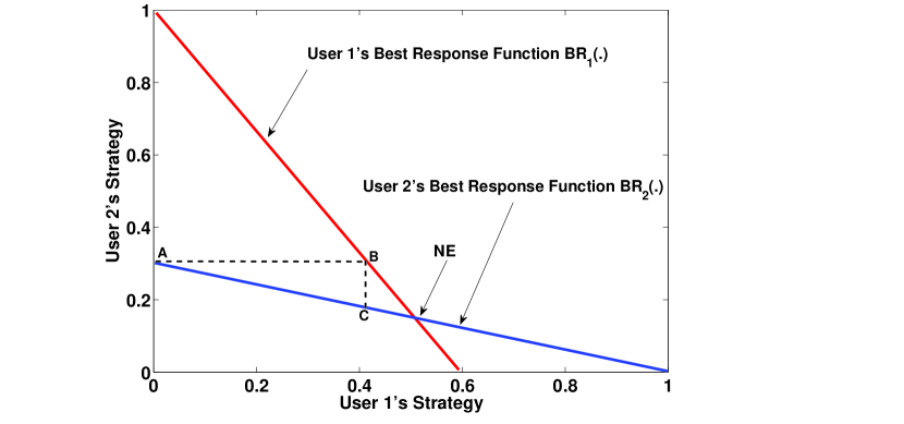
Figure 12: Illustration of the Nash Equilibrium (NE) of a 2-user scalar game. This figure also shows the process of a sequence of best responses that reach the NE. The function $BR_{k}(\cdot)$ represents user $k$’s best response function. Suppose both users initially choose $0$. User $2$ acts first and chooses point $A$ which is its best response, User $1$ acts next and chooses its best response point $B$. User $2$ acts again and chooses point $C$. Continuing iteratively in this fashion, the NE will be reached in the limit.

Let us illustrate the notion of NE in our 2-user scalar IC model (14). Suppose these two users are the players of a game, and their strategy spaces are $\chi_{k}=\{p_{k}\mid 0\leq p_{k}\leq\bar{p}_{k}\}$, $k=1,2$. Assume that the users’ utility functions are their maximum transmission rates defined in (18). Thus, for this example, user 1’s best response function admits a particular simple expression

$$BR_{1}(p_{2}) = \arg\max_{0\leq p_{1}\leq\bar{p}_{1}}\log_{2}\left(1+\frac{|H_{11}|^{2}p_{1}}{1+|H_{21}|^{2}p_{2}}\right)$$ (107)

$$= \bar{p}_{1}.$$

This says that regardless of user $2$’s transmission strategy, user $1$ will transmit with full power. The same can be said about user $2$. Consequently, the only NE of this game is the transmit power tuple $(\bar{p}_{1},\bar{p}_{2})$. Obviously, assuming that each user is indeed selfish and they intend to maximize their own utility, the NE point $(\bar{p}_{1},\bar{p}_{2})$ can be implemented without any explicit coordination between the users. Now let us assess the efficiency of such power allocation scheme in terms of system sum rate. In Fig. 14 and Fig. 14, we plot the rate region boundary and the NE points for different interference levels. We see that when interference is low, the NE corresponds exactly to the maximum sum rate point. However, when interference is strong, the NE scheme is inferior to the time sharing scheme in which the users transmit with full power in an orthogonal and interference free fashion (e.g., TDMA or FDMA). Nonetheless, it should be pointed out that the NE point can be reached without user coordination, while the time sharing scheme requires the users to synchronize their transmissions.

We refer the readers to the September 2009 issue of IEEE Signal Processing Magazine for the applications of game theory to wireless communication and signal processing.

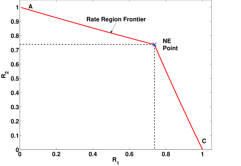
Figure 13: An illustration of the efficiency of the NE for 2-user IC when the interference is weak. $\bar{p}_{1}=\bar{p}_{2}=1$, $|H_{11}|^{2}=|H_{22}|^{2}=1,$ $|H_{12}|^{2}=|H_{21}|^{2}=0.5$, $\sigma^{2}_{1}=\sigma^{2}_{2}=1$. At point $A$ and $C$, a single user transmits using full power; at the NE point, both users transmit using full power.

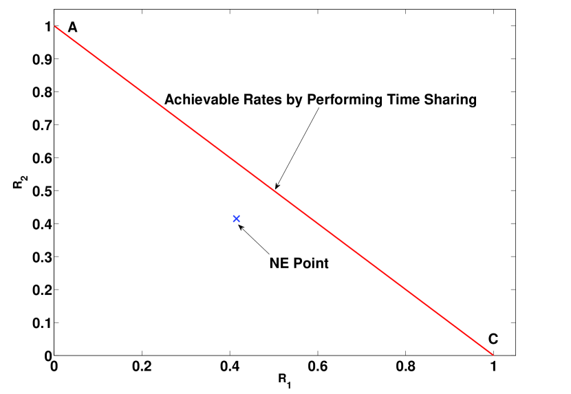
Figure 14: An illustration of the inefficiency of the NE for 2-user IC when the interference is strong. $\bar{p}_{1}=\bar{p}_{2}=1$, $|H_{11}|^{2}=|H_{22}|^{2}=1,$ $|H_{12}|^{2}=|H_{21}|^{2}=2$, $\sigma^{2}_{1}=\sigma^{2}_{2}=1$. At point $A$ and $C$, a single user transmits using full power; at the NE point, both users transmit using full power.

4.2    Distributed Resource Allocation for Interference Channels

Early works on distributed physical layer resource allocation in wireless networks largely deal with the scalar IC models. Sarayda et al. (2001), Sarayda et al. (2002) and Goodman Mandayam (2000) are among the first to cast the general scalar power control problem in a game theoretic framework. They proposed to quantify the tradeoff between the users’ QoS requirements and energy consumption by a utility function in the form:

$$U_{k}(p_{k},\mathbf{p}_{-k})=\frac{R_{k}f(\mbox{SINR}_{k})}{p_{k}}$$ (108)

where $R_{k}$ is user $k$’s fixed transmission rate, and $f(\mbox{SINR}_{k})$ is a function of user $k$’s SINR that characterizes its bit error rate (BER). They showed that any NE point is inefficient in the Pareto sense, i.e., it is possible to increase the utility of some of the terminals without hurting any other terminal. To improve the efficiency of the power control game, they proposed to charge the users with a price that is proportional to their transmit powers. Specifically, each users’ utility function now becomes $U_{k}(p_{k},\mathbf{p}_{-k})=R_{k}f\left(\mbox{SINR}_{k}\right)/p_{k}-\alpha_{k}p_{k}$, where $\alpha_{k}$ is a positive scalar that can be appropriately chosen by the system operator. They showed that this modified game always admits a NE, and proposed an algorithm that allows the users to reach one of the NEs by adapting their transmit powers in the best response fashion. Meshkati et al. (2006) and Meshkati et al. (2007) extended the above works to the multi-carrier data network. They defined the utility function for each user as

$$U_{k}(\mathbf{p}_{k},\mathbf{p}_{-k})=\frac{\sum_{n=1}^{N}R^{n}_{k}f_{k}(\mbox{SINR}^{n}_{k})}{\sum_{n=1}^{N}p^{n}_{k}}.$$ (109)

where the function $f_{k}(\cdot)$ represents the BER of user $k$, and it incorporates the underlying structure of different linear receivers. However, such multi-carrier power control game is more complicated than the scalar power control game introduced early, and in certain network configurations it is possible that no NE exists (see Meshkati et al. (2006)).

An alternative approach in distributed power control is to directly optimize the individual users’ transmission rates. Consider a $K$-user $N$-channel parallel IC model. Assume that each user $k\in\mathcal{K}$ is interested in maximizing its transmission rate, and again assume that its total transmission power budget is $\bar{p}_{k}$. Then the users’ utility functions as well as their feasible spaces can be expressed as

$$U_{k}(\mathbf{p}_{k},\mathbf{p}_{-k}) = \sum_{n=1}^{N}\log_{2}\left(1+\frac{|H^{n}_{kk}|^{2}p^{n}_{k}}{1+\sum_{l\neq k}|H^{n}_{lk}|^{2}p^{n}_{l}}\right),~{}k=1,\cdots,K,$$ (110)

$$\chi_{k} = \left\{\mathbf{p}_{k}\ \big{|}\ \sum_{n=1}^{N}p^{n}_{k}\leq\bar{p}_{k},p^{n}_{k}\geq 0,~{}n=1,\cdots,N\right\},~{}k=1,\cdots,K.$$ (111)

Fixing $\mathbf{p}_{-k}$, user $k$’s best response solution $\mathbf{p}_{k}^{*}$ is the classical water-filling (WF) solution

$$p^{n,*}_{k}=\left[\frac{1}{\lambda_{k}}-\frac{1+\sum_{l\neq k}|H^{n}_{lk}|^{2}p^{n}_{l}}{|H^{n}_{kk}|^{2}}\right]^{+},~{}n=1,\cdots,N$$ (112)

where $\lambda_{k}\geq 0$ is the dual variable ensuring the sum power constraint, and the operator $[x]^{+}=\max\{x,0\}$. Figure 15 illustrates the WF solution for user $k$. We note that in order to compute the WF solution, user $k$ needs to know the terms $\{1+\sum_{l\neq k}|H^{n}_{lk}|^{2}p^{n}_{l}\}_{n=1}^{N}$, which is simply the set of noise-plus-interference (NPI) levels on all its channels. They can be measured locally at its receiver.

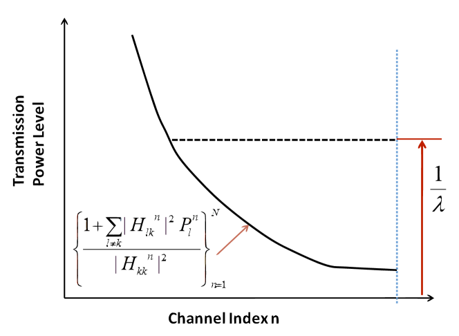
Figure 15: Illustration of the Water-Filling computation for user $k$.

We refer to this game as a WF game.

Yu et al. (2002) is the first to formulate the distributed power control problem as a WF game. The authors proposed an iterative water-filling algorithm (IWFA) in which the following two steps are performed iteratively:

1) each user $k\in\mathcal{K}$ measures its NPI power $\{1+\sum_{l\neq k}|H^{n}_{lk}|^{2}p^{n,(t)}_{l}\}_{n=1}^{N}$; 2) each user $k\in\mathcal{K}$ computes its power allocation $\mathbf{p}^{(t+1)}_{k}$ according to (112).

Variations of the IWFA algorithm allow the users to update using different schedules. The following three update schemes have been proposed: a) simultaneous update, in which all the users update their power in each iteration, see Yu et al. (2002) and Scutari et al. (2008d); b) sequential update, in which a single user updates in each iteration, see Luo Pang (2006) and Scutari et al. (2008d); c) asynchronous update, in which a random fraction of users update in each iteration, and they are allowed to use outdated information in their computation, see Scutari et al. (2008a). Regardless of the specific update schedule used, the IWFA algorithm is a distributed algorithm because only local NPI measurements are needed for the users to perform their independent power update.

The properties of the WF game as well as the convergence conditions of the IWFA have been extensively studied. The original work has only provided sufficient conditions for the convergence of the IWFA in a 2-user network. Subsequent works such as Luo Pang (2006), Shum et al. (2007), Cendrillon et al. (2007), Scutari et al. (2008c) and Scutari et al. (2008d) generalized this result to networks with arbitrary number of users. Luo Pang (2006) characterized the NE of the water-filling game as the solution to the following affine variational inequality (AVI)

$$(\mathbf{p}^{{}^{\prime}}-\mathbf{p})(1+\mathbf{M}\mathbf{p})\geq 0,~{}\forall~{}\mathbf{p}^{{}^{\prime}}\in\chi,$$ (113)

where $\mathbf{M}$ is a block partitioned matrix with its $(ij)^{th}$ block defined as $\mathbf{M}^{ij}=\mbox{diag}\left(\frac{|H^{1}_{ji}|^{2}}{|H^{1}_{ii}|^{2}},\cdots,\frac{|H^{N}_{ji}|^{2}}{|H^{N}_{ii}|^{2}}\right)$. Using the AVI characterization (113), they also showed that the sequential version of the IWFA corresponds to the classical projection algorithm whose convergence to the unique NE of the water-filling game is guaranteed if the following contraction condition is satisfied

$$\rho\left(\left(\mathbf{I}-{\mbox{\boldmath$\Upsilon$}}_{low}\right)^{-1}{\mbox{\boldmath$\Upsilon$}}_{upp}\right)<1$$ (114)

where ${\mbox{\boldmath$\Upsilon$}}_{low}$ and ${\mbox{\boldmath$\Upsilon$}}_{upp}$ is the strictly lower and strictly upper triangular part of a $K\times K$ matrix $\Upsilon$ given by

$$[{\mbox{\boldmath$\Upsilon$}}]_{q,r}\triangleq\left\{\begin{array}[]{ll}\max_{n}\left\{\frac{|H^{n}_{rq}|^{2}}{|H^{n}_{qq}|^{2}}\right\}&\textrm{if }r\neq q\\ 0&\textrm{otherwise. }\\ \end{array}\right.$$ (117)

Also using the AVI characterization (113), the authors of Scutari et al. (2008c) and Scutari et al. (2008d) further proved that the condition

$$\rho\left({\mbox{\boldmath$\Upsilon$}}\right)<1$$ (118)

is sufficient for the convergence of the IWFA as well as the uniqueness of the NE. We refer the readers to Scutari et al. (2008b) for a detailed comparison of various conditions for the convergence of the IWFA. It is worth noticing that all the sufficient conditions for the convergence of IWFA require that the interference among the users are weak. For example, a sufficient condition for (118) is

$$\sum_{l\neq k}|H^{n}_{kl}|^{2}s_{k}<{|H^{n}_{ll}|^{2}}s_{l},~{}\forall~{}k\in\mathcal{K},~{}n\in\mathcal{N}$$ (119)

where $s_{k}>0,k=1,\cdots,K$ is a set of constant scalars. Intuitively, this condition says that at the receiver of each user $k\in\mathcal{K}$, the power of the useful signal should be larger than the power of total interference. When the interference is strong, IWFA diverges. Leshem Zehavi (2009) provided an example in which all forms of IWFA diverge, regardless of their update schedules. We remark that extending the IWFA so that it converges in less stringent conditions that do not require the interference to be weak is still an open problem. Without any algorithmic modifications, the standard IWFA is only known to converge (Luo Pang (2006)) when the crosstalk coefficients are symmetric

$$\frac{|H^{n}_{rq}|^{2}}{|H^{n}_{qq}|^{2}}=\frac{|H^{n}_{qr}|^{2}}{|H^{n}_{rr}|^{2}},\quad\forall\ r\neq q,\ \forall\ n,$$

regardless the interference levels.

The IWFA has been recently generalized to MIMO IC model. In the MIMO WF game, the strategy of each user $k\in\mathcal{K}$ is its transmission covariance matrix $\mathbf{Q}_{k}$. The rate utility function and strategy set for user $k$ can be expressed as

$$U_{k}(\mathbf{Q}_{k},\mathbf{Q}_{-k}) = \log_{2}\det\left(\mathbf{H}_{kk}\mathbf{Q}_{k}\mathbf{H}_{kk}^{H}\left(\mathbf{I}_{N_{r}}+\sum_{l\neq k}\mathbf{H}_{lk}\mathbf{Q}_{l}\mathbf{H}_{lk}^{H}\right)^{-1}+\mathbf{I}_{N_{r}}\right)$$ (120)

$$\chi_{k} = \left\{\mathbf{Q}_{k}:\mbox{Tr}(\mathbf{Q}_{k})\leq\bar{p}_{k},\mathbf{Q}_{k}\succeq 0\right\}.$$ (121)

In this case, each user $k$’s best response $BR_{k}(\mathbf{Q}_{-k})$ is again a water-filling solution, see Telatar (1999). Arslan et al. (2007) suggested that in each iteration, the users’ covariance can be updated as

$$\mathbf{Q}^{(t+1)}_{k}=\alpha_{t}\mathbf{Q}^{(t)}_{k}+(1-\alpha_{t})BR_{k}(\mathbf{Q}^{t}_{-k})$$ (122)

where $\{\alpha_{t}\}_{t=1}^{\infty}$ is a set of constants that satisfy $\alpha_{t}\geq 0$, $\lim_{t\to\infty}\alpha_{t}=0$ and $\lim_{t\to\infty}\sum_{t=1}^{T}\alpha_{t}<\infty$. They claimed that their algorithm converges when the interference is weak, but no specific conditions are given. This work has been generalized by Scutari et al. (2008b) and Scutari et al. (2009), in which rigorous conditions for the convergence of the MIMO IWFA have been derived. In particular, consider a MIMO network in which $N_{t}=N_{r}$ and the direct link channel matrices $\{\mathbf{H}_{kk}\}_{k=1}^{K}$ are all nonsingular. Define a $K\times K$ matrix $\mathbf{S}$ as

$$[\mathbf{S}]_{q,r}\triangleq\left\{\begin{array}[]{ll}\rho\left(\mathbf{H}^{H}_{rq}\mathbf{H}^{-H}_{qq}\mathbf{H}^{-1}_{qq}\mathbf{H}_{rq}\right)&\textrm{if }r\neq q\\ 0&\textrm{otherwise. }\\ \end{array}\right.$$ (125)

Then the condition $\rho\left(\mathbf{S}\right)<1$ is sufficient for the convergence of the sequential/simultaneous/asynchronous MIMO IWFA. This condition is again a weak interference condition, and future work is needed to extend the MIMO IWFA to work in networks without this restriction. We refer the readers to web pages of Yu, Palomar and Pang for other works related to the WF games and IWFA.

The above parallel and MIMO WF games have been extended in several directions. A series of recent works considered the robustness issue in a WF games. For instance, Gohary et al. (2009) considered the WF game in the presence of a jammer. Let us denote user $0$ as the jammer and denote its transmission power as $\mathbf{p}_{0}=\left[p^{1}_{0},\cdots,p^{N}_{0}\right]^{T}$. The rate utility function of a normal user $k$ ($k\neq 0$) becomes

$$U_{k}(\mathbf{p}_{k},\mathbf{p}_{-k},\mathbf{p}_{0})=\sum_{n=1}^{N}\log_{2}\left(1+\frac{|H^{n}_{kk}|^{2}p^{n}_{k}}{1+\sum_{l\neq k}|H^{n}_{lk}|^{2}p^{n}_{l}+|H^{n}_{0k}|^{2}p^{n}_{0}}\right).$$ (126)

Suppose the jammer’s objective is to minimize the utility of the whole system. This can be reflected by its utility function and the strategy set

$$U_{0}(\mathbf{p}_{0},\mathbf{p}) = -\sum_{k=1}^{K}U_{k}(\mathbf{p}_{k},\mathbf{p}_{-k},\mathbf{p}_{0})$$ (127)

$$\chi_{0} = \left\{\mathbf{p}_{0}:\sum_{n=1}^{N}p^{n}_{0}\leq\bar{p}_{0},p^{n}_{0}\geq 0,\forall~{}n\in\mathcal{N}\right\}.$$ (128)

Gohary et al. (2009) proposed a generalized IWFA (GIWFA) algorithm in which the normal users and the jammer all selfishly maximize their respective utility functions. Notice that the selfish maximization problems are all convex. The convergence condition for the GIWFA is

$$\rho\left(\left(\mathbf{I}-{\mbox{\boldmath$\Upsilon$}}_{low}\right)^{-1}{\mbox{\boldmath$\Upsilon$}}_{upp}\right)\leq\frac{1}{1+a}-c<1$$ (129)

where the matrix $\Upsilon$ is defined in (117), and $a>0$ and $c>0$ are constants related to the system parameters. Clearly this condition is more restrictive than those of the original IWFA, for example the condition (114). This is partly because the presence of the jammer introduces uncertainty to the NPI that each normal user experiences.

Uncertainty of the NPI is also caused by events such as sudden changes in the number of users in the system or errors of interference measurement at the receivers. Setoodeh Haykin (2009) seek a formulation that takes into consideration the worst case NPI errors. Let ${I}^{n}_{k}$ denote the power of NPI that user $k$ should have experienced on channel $n$ if no measurement errors occur. Let $\tilde{{I}}^{n}_{k}={I}^{n}_{k}-\Delta{I}^{n}_{k}$ be the measured NPI value, with $\Delta{I}^{n}_{k}$ representing the NPI uncertainty. Let $\Delta\mathbf{I}_{k}=\left[\Delta{I}^{n}_{1},\cdots,\Delta{I}^{n}_{K}\right]^{T}$ and suppose it is bounded, i.e., $\|\Delta\mathbf{I}_{k}\|\leq\epsilon_{k}$ for some $\epsilon_{k}>0$. In this robust WF game, the objectives of the users are to maximize their worst case transmission rate. In other words, user $k$’s utility function can be expressed as

$$U_{k}(\mathbf{p}_{k},\mathbf{p}_{-k})=\min_{\|\Delta\mathbf{I}_{k}\|\leq\epsilon_{k}}\sum_{n=1}^{N}\log_{2}\left(1+\frac{|H^{n}_{kk}|^{2}p^{n}_{k}}{\tilde{{I}}^{n}_{k}+\Delta{I}^{n}_{k}}\right).$$ (130)

This formulation trades performance in favor of robustness, thus the equilibrium solution obtained is generally less efficient than that of the original IWFA. In Hong Garcia (2011a), an averaged version of IWFA was proposed which converges when the error of the NPI $\Delta\mathbf{I}_{k}$ satisfies certain conditions. In Gohary Willink (2009), the authors provided a probabilistically robust IWFA to deal with the quantization errors of the NPI at the receiver of each user. In this algorithm, users allocate their powers to maximize their total rate for a large fraction of the error realization.

Another thread of works such as Xie et al. (2010), Wu Tsang (2008), Hong Garcia (2011b), Wang et al. (2011) and Pang et al. (2010) generalized the original WF game and the IWFA to interfering cognitive radio networks (CRN). In a CRN, the secondary users (SUs) are allowed to use the spectrum that is assigned to the primary users (PUs) as long as the SUs do not create excessive interference to the primary network. Suppose the secondary network is a $K$-user $N$-channel parallel IC. Let $\mathcal{Q}=\{1,\cdots,Q\}$ denote the set of PUs in the network. Let $|G^{n}_{kq}|^{2}$ denote the channel gain from SU $k$ to PU $q$ on channel $n$. The following aggregated interference constraints are imposed on the secondary network (these constraints are also referred to as the interference temperature-constraints, see FCC (2003) and Zhang et al. (2010))

$$\sum_{k=1}^{K}|G^{n}_{kq}|^{2}p_{k}\leq\bar{I}^{n}_{q},~{}\forall~{}(q,n)\in\mathcal{Q}\times\mathcal{N}$$ (131)

where $\bar{I}^{n}_{q}$ represents the maximum aggregated interference allowed at the receiver of PU $q$ on channel $n$. The original WF algorithm needs to be properly modified to strictly enforce these interference constraints in the equilibrium. Xie et al. (2010) formulated the power allocation problem in this CRN as a competitive market model. In this model, each channel has a fictitious price per unit power, and the users must purchase the transmission power on each channel to maximize their data rates. Scutari et al. (2010) and Scutari et al. (2009) systematically studied the WF game with interference constraints. For each primary user $q$, they introduced a set of interference prices ${\mbox{\boldmath$\nu$}}_{q}=\left[\nu_{q}^{1},\cdots,\nu_{q}^{N}\right]^{T}$. Each SU is charged for their contribution of total interference at PUs’ receiver. Specifically, a SU $k$’s utility function and feasible set is defined as

$$U_{k}(\mathbf{p}_{k},\mathbf{p}_{-k},{\mbox{\boldmath$\nu$}})=R_{k}(\mathbf{p}_{k},\mathbf{p}_{-k})-\sum_{q=1}^{Q}\sum_{n=1}^{N}\nu^{n}_{q}|G^{n}_{kq}|^{2}p^{n}_{k},$$ (132)

$$\chi_{k}=\left\{\mathbf{p}_{k}:\sum_{n=1}^{N}p^{n}_{k}\leq\bar{p}_{k},p^{n}_{k}\geq 0,~{}n=1,\cdots,N\right\}$$ (133)

where $R_{k}(\mathbf{p}_{k},\mathbf{p}_{-k})$ is user $k$’s transmission rate. The NE of this interference-constrained WF game is the tuple $({\mbox{\boldmath$\nu$}}^{*},\mathbf{p}^{*})$ that satisfies the following conditions

$$\mathbf{p}_{k}^{*}=\max_{\mathbf{p}_{k}\in\chi_{k}}U_{k}(\mathbf{p}_{k},\mathbf{p}^{*}_{-k},{\mbox{\boldmath$\nu$}}^{*}),$$

$$\sum_{k=1}^{K}|G^{n}_{kq}|^{2}p^{n,*}_{k}\leq\bar{I}_{q}^{n},~{}(q,n)\in\mathcal{Q}\times\mathcal{N}$$

$$\nu^{n,*}_{q}(\bar{I}_{q}^{n}-\sum_{k=1}^{K}|G^{n}_{kq}|^{2}p^{n,*}_{k})=0,\ \nu^{n,*}_{q}\geq 0,\ ~{}(q,n)\in\mathcal{Q}\times\mathcal{N}.$$

Scutari et al. (2010) and Scutari et al. (2009) derived the conditions for the existence and uniqueness of the NE for this game. Introduce a $N\times N$ matrix $\widehat{{\mbox{\boldmath$\Upsilon$}}}$

$$[\widehat{{\mbox{\boldmath$\Upsilon$}}}]_{l,k}\triangleq\left\{\begin{array}[]{ll}-\max_{n\in\mathcal{N}}\left\{\frac{|H^{n}_{lk}|^{2}}{|H^{n}_{kk}|^{2}}\times\widehat{\mbox{innr}}^{n}_{lk}\right\}&\textrm{if }k\neq l\\ 1&\textrm{otherwise }\\ \end{array}\right.$$ (136)

where $\widehat{\mbox{innr}}^{n}_{lk}\triangleq 1+\sum_{m\in\mathcal{K}}|H^{n}_{km}|^{2}\bar{p}_{k}$. Then the condition $\widehat{{\mbox{\boldmath$\Upsilon$}}}\succeq 0$ guarantees the uniqueness of the NE. A set of distributed algorithms that alternately update the users’ power allocation and the interference prices were proposed to reach the NE of this game. The MIMO generalization has been considered in Scutari Palomar (2010), whereby both the SUs and PUs are equipped with multiple antennas. Another extension Wang et al. (2011) considered the possibility that the SU-PU channels may be uncertain, and formulated a robust WF game that ensures the SU-PU interference constraints are met even in the worst case channel conditions.

All the above mentioned WF games can be categorized as rate adaptive (RA) games, in which the users selfishly maximize their own data rates. One drawback of the RA formulation is that individual users have no QoS guarantees. Alternatively, a fixed margin (FM) formulation allows each user to minimize its transmission power while maintaining its QoS constraint. The FM formulation is more difficult to analyze due to the coupling of the users’ strategy spaces resulted from the QoS constraint. For the parallel IC model, the utility function and the strategy set for user $k$ in a FM formulation can be expressed as

$$U_{k}(\mathbf{p}_{k}) = -\sum_{n=1}^{N}p^{n}_{k}$$ (137)

$$\chi_{k}(\mathbf{p}_{-k}) = \left\{\mathbf{p}_{k}:R_{k}(\mathbf{p}_{k},\mathbf{p}_{-k})\geq\zeta_{k},p^{n}_{k}\geq 0,n\in\mathcal{N}\right\}$$ (138)

where $\zeta_{k}$ is the rate target for user $k$. The solution to the individual users’ utility maximization problems, assuming the feasibility of the rate targets, is again a water-filling solution

$$p^{n,*}_{k}=\left[{\lambda_{k}}-\frac{1+\sum_{l\neq k}|H^{n}_{lk}|^{2}p^{n}_{l}}{|H^{n}_{kk}|^{2}}\right]^{+},~{}n=1,\cdots,N$$ (139)

where $\lambda_{k}$ is the water-level that is associated with user $k$’s rate constraint.

A NE of this FM game (which is usually referred to as the generalized NE due to the coupling of the users’ strategy spaces) is defined as a power vector $\mathbf{p}^{*}$ that satisfies

$$\mathbf{p}^{*}_{k}\in\arg\max_{\mathbf{p}_{k}\in\chi_{k}(\mathbf{p}^{*}_{-k})}U_{k}\left(\mathbf{p}_{k},\mathbf{p}^{*}_{-k}\right),~{}k=1,\cdots,K.$$ (140)

Similar to the min-power QoS constrained formulation discussed in the previous section, the first thing we need to characterize for this FM game is the feasibility of a given set of rate targets. The following condition is among many of those that have been derived in Pang et al. (2008) which guarantee the existence of a bounded power allocation achieving the given set of rate targets

$$\sum_{l\neq k}\frac{|H^{n}_{kl}|^{2}}{|H^{n}_{kk}|^{2}}<\frac{1}{\exp\{\zeta_{k}\}-1},~{}(n,k)\in\mathcal{N}\times\mathcal{K}.$$ (141)

This condition is again a weak interference condition. The following condition is sufficient for the uniqueness of the (generalized) NE of the FM game

$$\sum_{l\neq k}\max_{n\in\mathcal{N}}\left\{\frac{|H^{n}_{kl}|^{2}}{|H^{n}_{kk}|^{2}}\right\}<\frac{\beta}{\exp\{\zeta_{l}\}-1},~{}k\in\mathcal{K}$$ (142)

where $\beta<1$ is related to the set of given rate targets. This condition is also sufficient for the convergence of a FM-IWFA in which the users sequentially or simultaneously update their power using the WF solution. Algorithmic extension of this work to the CRN with interference constraints of the form (131) has been considered recently in Wu Tsang (2009). It remains to see how the FM games and their theoretical properties (e.g., uniqueness of the NE, convergence of the FM-IWFA) can be extended to MIMO CRNs with interference constraints.

We remark that the NE points of the various RA based WF games introduced in this section is generally inefficient, in the sense that the sum rate of the users is often smaller compared with that of the socially optimal solutions. In Fig. 16, we illustrate such inefficiency of the NE in a parallel IC with $K=2$, $N=32$ and randomly generated channel coefficients. We plot the NE point of the WF game as well as the rate region boundary achieved by the SCALE algorithm. In order to improve the efficiency of the NE, user coordination must be incorporated into the original WF game. The pricing algorithms such as MDP, M-IWF or WMMSE introduced in the previous section are examples of such extensions. In those algorithms, system efficiency is improved due to explicit message exchange and cooperation among the users. Careful analysis is needed to identify the tradeoffs between the improvement of the system sum rate and the signalling overhead. Evidently, when the total number of users in the system is large, a complete cooperation of all users is too costly. An interesting problem is to decide how to partition the users into collaborative groups in a way that strike an optimal tradeoff between system performance and coordination overhead.

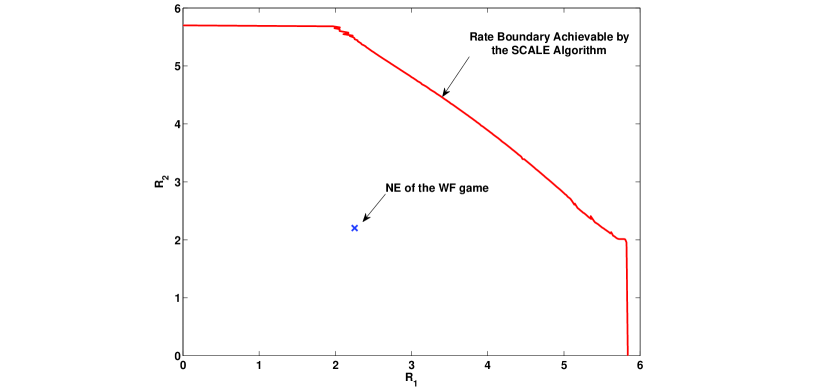
Figure 16: Illustration of the inefficiency of the NE point for a WF game with $K=2$, $N=32$ and $\bar{p}_{1}=\bar{p}_{2}=1$.

5   Resource Allocation via Interference Alignment

Theoretically, the optimal resource allocation for a MIMO interference channel is related to the characterization of the capacity region of an interference channel, i.e., determining the set of rate tuples that can be achieved by the users simultaneously. In spite of intensive research on this subject over the past three decades, the capacity region of interference channels is still unknown (even for small number of users). The lack of progress to characterize the capacity region of the MIMO interference channel has motivated researchers to derive various approximations of the capacity region. For example, the maximum total degrees of freedom (DoF) corresponds to the first order approximation of sum-rate capacity in the high SNR regime. Specifically, in a $K$-user interference channel, we define the degrees of freedom region as the following Cadambe Jafar (2008b):

$$\begin{array}[]{ll}\mathcal{D}=\bigg{\{}&\!\!\displaystyle(d_{1},d_{2},\ldots,d_{K})\in\mathbb{R}_{+}^{K}\ \;\bigg{|}\ \;\forall(w_{1},w_{2},\ldots,w_{K})\in\mathbb{R}_{+}^{K},\\ &\displaystyle\sum_{k=1}^{K}w_{k}d_{k}\leq\limsup_{{\rm SNR}\rightarrow\infty}\left[\sup_{\mathbf{R}\in\mathcal{C}}\frac{1}{\log{\rm SNR}}\sum_{k=1}^{K}w_{k}R_{k}\right]\ \ \bigg{\}},\end{array}$$ (143)

where $\mathcal{C}$ is the capacity region and $R_{k}$ is the rate of user $k$. The total DoF in the system can be defined as the following:

$$\eta=\max_{(d_{1},d_{2},\ldots,d_{K})\in\mathcal{D}}d_{1}+d_{2}+\ldots+d_{K}.$$

Roughly speaking, the total DoF is the number of independent data streams that can be communicated in the channel without interference.

For various channel models, the DoF region or the total DoF have been characterized recently. In particular, for a point-to-point MIMO channel with $M$ antennas at the transmitter and $N$ antennas at the receiver, the total DoF is $\eta=\min\{M,N\}$. Different approaches such as SVD precoder or V-BLAST can be used to achieve this DoF bound. For a 2-user MIMO fading interference channel with user $k$ equipped with $M_{k}$ transmit antennas and $N_{k}$ receive antennas ($k=1,2$), Jafar Fakhereddin (2007) proves that the maximum total DoF is

$$\eta=\min\left\{M_{1}+M_{2},N_{1}+N_{2},\max\{M_{1},N_{2}\},\max\{M_{2},N_{1}\}\right\}.$$

Therefore, for the case of $M_{1}=M_{2}=N_{1}=N_{2}$, the total DoF in the system is the same as the single user case. In other words, we do not gain more DoF by increasing the number of users from one to two. Interestingly, if generic channel extensions (drawn from a continuous probability distribution) are allowed either across time or frequency, Cadambe Jafar (2008b) showed that the total DoF is $\eta={KM}/{2}$ for a $K$-user MIMO interference channel, where $M$ is the number of transmit/receive antennas per user. This surprising result implies that each user can effectively utilize half of the total system resources in an interference-free manner by aligning the interference at all receivers. Moreover, this total DoF can be achieved by using a carefully designed linear beamforming strategy.

Mathematically, a linear beamforming strategy for a $K$-user MIMO IC can be described by the transmit beamforming matrices $\{\mathbf{V}_{k}\}_{k\in{\cal K}}$ and the receive beamforming matrices $\{\mathbf{U}_{k}\}_{k\in{\cal K}}$. The receiver $k$ estimates the transmitted data vector $\mathbf{s}_{k}$ as follows

$$\mathbf{x}_{k}=\mathbf{V}_{k}\;\mathbf{s}_{k},\;\;\;\;\;\;\;\hat{\mathbf{s}}_{k}=\mathbf{U}_{k}^{H}\mathbf{y}_{k}$$

where the power of the data vector $\mathbf{s}_{k}\in\mathcal{R}^{d_{k}\times 1}$ is normalized such that $E[\mathbf{s}_{k}\mathbf{s}_{k}^{H}]=\mathbf{I}$, and $\hat{\mathbf{s}}_{k}$ is the estimate of $\mathbf{s}_{k}$ at the $k$-th receiver. The matrices $\mathbf{V}_{k}\in\mathcal{C}^{M_{k}\times d_{k}}$ and $\mathbf{U}_{k}\in\mathcal{C}^{N_{k}\times d_{k}}$ are the beamforming matrices at the $k$-th transmitter and receiver respectively, where $M_{k}$ ($N_{k}$) is the number of antennas at transmitter $k$ (respectively receiver $k$). Without channel extension, the linear interference alignment conditions can be described by the following zero-forcing conditions Yetis et al. (2010); Razaviyayn et al. (2011a)

$$\mathbf{U}_{k}^{H}\mathbf{H}_{jk}\mathbf{V}_{j}=0,\;\;\;\;\ k=1,\cdots,K,\ \forall\ j\neq k,$$ (144)

$$\mbox{rank}\left(\mathbf{U}_{k}^{H}\mathbf{H}_{kk}\mathbf{V}_{k}\right)=d_{k},\quad\ k=1,\cdots,K.$$ (145)

The first equation guarantees that all the interfering signals at receiver $k$ lie in the subspace orthogonal to $\mathbf{U}_{k}$, while the second one assures that the signal subspace $\mathbf{H}_{kk}\mathbf{V}_{k}$ has dimension $d_{k}$ and is linearly independent of the interference subspace. Clearly, as the number of users $K$ increases, the number of constraints on the beamformers $\{\mathbf{U}_{k},\mathbf{V}_{k}\}$ increases quadratically in $K$, while the number of design variables in $\{\mathbf{U}_{k},\mathbf{V}_{k}\}$ only increases linearly. This suggests the above interference alignment can not have a solution unless $K$ or $d_{k}$ is small.

If the interference alignment conditions (144) and (145) hold for some linear beamforming matrices $\{\mathbf{V}_{k},\mathbf{U}_{k}\}_{k\in\mathcal{K}}$, then transmitter $k$ can use $\mathbf{V}_{k}$ to send $d_{k}$ independent data streams to receiver $k$ (per channel use) without any interference. Thus, $d_{k}$ represents the DoF achieved by the $k$-th transmitter/receiver pair in the information theoretic sense of (143). In other words, the vector $(d_{1},d_{2},...,d_{K})$ in (144) and (145) represents the tuple of DoF achieved by linear interference alignment. Intuitively, the larger the values of $d_{1},d_{2}$,…,$d_{K}$, the more difficult it is to satisfy the interference alignment conditions (144) and (145).

In principle, we can allocate resources by maximizing the total achievable DoF. In particular, for a specific channel realization $\{\mathbf{H}_{kj}\}_{k,j\in\mathcal{K}}$, we need to find the beamforming matrices $\{\mathbf{V}_{k},\mathbf{U}_{k}\}$ to maximize the total DoF while satisfying (144)–(145).

$$\begin{array}[]{ll}\displaystyle\max_{\{\mathbf{U}_{k},\mathbf{V}_{k}\}_{k=1}^{K}}&\displaystyle\sum_{k=1}^{K}{d_{k}}\\ \mbox{subject to}&\displaystyle\mathbf{U}_{k}^{H}\mathbf{H}_{kj}\mathbf{V}_{j}=0\;\;\;\;\;\;k=1,..,K,\;\;j\neq k\\ &\mbox{rank}\left(\mathbf{U}_{k}^{H}\mathbf{H}_{kk}\mathbf{V}_{k}\right)=d_{k}\;\;\;\;\;\;k=1,..,K\end{array}$$

Unfortunately, according to Razaviyayn et al. (2011a), this problem is NP-hard. So we are led to find suboptimal solution for this problem. However, no efficient algorithms have been developed to approximately solve this problem at this point.

Instead of maximizing the total DoF, we can focus on a seemingly simpler problem: for a given channel realization $\{\mathbf{H}_{kj}\}_{k,j\in\mathcal{K}}$ and a fixed DoF tuple $\mathbf{d}=(d_{1},...,d_{K})$, check if there exist linear beamformers $\{\mathbf{V}_{k},\mathbf{U}_{k}\}_{k\in\mathcal{K}}$ satisfying the alignment conditions (144)–(145). Notice that the conditions (144)–(145) are quadratic polynomial equations, which are difficult to solve in general. However, if we fix either $\{\mathbf{U}_{k}\}_{k\in\mathcal{K}}$ or $\{\mathbf{V}_{k}\}_{k\in\mathcal{K}}$, the quadratic equations become linear and can be solved via the linear least squares. This suggests the following alternating directions method for solving (144)–(145) (for a fixed $\mathbf{d}$):

1) Fix the transmit beamformers $\{\mathbf{V}_{k}\}_{k\in\mathcal{K}}$. Each receiver $k$ solves the following optimization problem $$\begin{array}[]{ll}\min&\displaystyle\mbox{Tr}\left(\mathbf{U}_{k}^{H}\mathbf{Q}_{k}\mathbf{U}_{k}\right)\\ \mbox{s.t.}&\displaystyle\mathbf{U}_{k}^{H}\mathbf{U}_{k}=\mathbf{I}_{d_{k}}\end{array}$$ where $\mathbf{Q}_{k}=\sum_{j\neq k}\frac{p_{j}}{d_{j}}\mathbf{H}_{kj}\mathbf{V}_{j}\mathbf{V}_{j}^{H}\mathbf{H}_{kj}^{H}$, with $I_{k}=\mbox{Tr}\left(\mathbf{U}_{k}^{H}\mathbf{Q}_{k}\mathbf{U}_{k}\right)$ being the total received interference power, and ${\bar{p}}_{j}$ being the power budget of $j$-th transmitter. 2) Fix $\{\mathbf{U}_{k}\}_{k\in\mathcal{K}}$ and update the transmit beamformers $\{\mathbf{V}_{k}\}_{k\in\mathcal{K}}$ in a symmetric fashion as in step 1) (by exchanging the roles of transmitter and receiver, and replacing the channel matrices $\{\mathbf{H}_{k,j}\}_{k,j\in\mathcal{K}}$ by $\{\mathbf{H}^{H}_{kj}\}_{kj\in\mathcal{K}}$) 3) Repeat steps 1) and 2) until convergence.

Notice that the optimal solution $\mathbf{U}_{k}^{*}$ for (1)) is given by the eigen-vectors of $\mathbf{Q}_{k}$ corresponding to the $d_{k}$-smallest eigen-values. The above algorithm is proposed first in K. Gomadam Jafar (2008) and later in Peters Heath (2009), albeit from a different perspective. Obviously, this algorithm cannot converge if the DoF vector $\mathbf{d}$ is not achievable. However, even if $\mathbf{d}$ is achievable, there has been no formal analysis that shows this alternating direction algorithm indeed will converge.

The lack of formal convergence proof may not be surprising. In fact, according to Razaviyayn et al. (2011a), even checking the feasibility of (144)–(145) is NP-hard when each transmitter/receiver is equipped with at least 3 antennas. Hence, for a given channel realization, assigning DoFs to the users in a manner that ensures feasibility is not easy. However, when the number of antennas at each transmitter/receiver is at most 2, the problem of checking feasibility is polynomial time solvable (Razaviyayn et al. (2011a)).

Now let us turn our attention to the generic solvability of the interference alignment problem (144)-(145). In other words, we focus on the existence of a beamforming solution to the quadratic polynomial equations (144)-(145) when the channel matrices are randomly generated. To this end, it is natural to count the number of scalar equations and the number of scalar variables in the conditions (144)-(145). It is tempting to conjecture that there is an interference alignment solution if and only if the number of constraints is no larger than the number of variables (see Yetis et al. (2010)). Recently, Razaviyayn et al. (2011c) and Bresler et al. (2011) have settled this conjecture completely in one direction, and partially in the other direction. They derive a general condition, described below, that must be satisfied by any DoF tuple $(d_{1},d_{2},...,d_{K})$ achievable through linear interference alignment.

Let us denote the polynomial equations in (145) by the index set

$$\mathcal{J}\triangleq\{(k,j)\mid 1\leq k\neq j\leq K\}.$$

The following result (Razaviyayn et al. (2011c) and Bresler et al. (2011)) provides an upper bound on the total achievable DoF when no channel extension is allowed. Consider a $K$-user flat fading MIMO interference channel where the channel matrices $\{\mathbf{H}_{ij}\}_{i,j=1}^{K}$ are generic (e.g., drawn from a continuous probability distribution). Assume no channel extension is allowed. Then any tuple of degrees of freedom $(d_{1},d_{2},...,d_{K})$ that is achievable through linear interference alignment (144) and (145) must satisfy the following inequalities

$$\min\{M_{k},N_{k}\}\geq d_{k},\quad\forall\;k,$$ (146)

$$\max\{M_{k},N_{j}\}\geq d_{k}+d_{j},\quad\forall\;k,j,k\neq j,$$ (147)

$$\sum_{k:(k,j)\in\mathcal{I}}(M_{k}-d_{k})d_{k}+\sum_{j:(k,j)\in\mathcal{I}}(N_{j}-d_{j})d_{j}\geq\sum_{(k,j)\in\mathcal{I}}d_{k}d_{j},\quad\forall\;\mathcal{I}\subseteq\mathcal{J}.$$ (148)

Roughly, the left hand side of (148) is equal to the number of independent scalar variables in (144)-(145) and the right hand side of (148) corresponds to the number of constraints in (144). Thus, the necessity of condition (148) for the existence of a feasible alignment scheme can be understood by counting the dimensions. However, a formal proof of this condition requires the use of field extension theory (Razaviyayn et al. (2011c)). We remark that condition (148) can be used to bound the total DoF achievable in a MIMO interference channel. In particular, the following upper bounds follow directly from condition (148).

1. In the case of $d_{k}=d$ for all $k$, interference alignment is impossible unless

   $$d\leq\frac{1}{K(K+1)}\sum_{k=1}^{K}(M_{k}+N_{k}).$$

2. In the case of $M_{k}+N_{k}=M+N$, interference alignment requires

   $$\left(\sum_{k=1}^{K}d_{k}\right)^{2}+\sum_{k=1}^{K}d_{k}^{2}\leq(M+N)\sum_{k=1}^{K}d_{k}$$

   which further implies

   $$\sum_{k=1}^{K}d_{k}<(M+N).$$

The principal assumption enabling the surprising result of Cadambe Jafar (2008b) is that the channel extensions are exponentially long in $K^{2}$ and are generic (e.g., drawn from a continuous probability distribution). If no channel extensions are allowed, part (b) above shows that the total achievable DoF in a MIMO interference channel is bounded by a constant $M+N-1$, regardless of how many users are present in the system. While this bound is an improvement over the single user case which has a maximum DoF of $\min\{M,N\}$, it is significantly weaker than the maximum achievable total DoF of $K/2$ for a diagonal frequency selective (or time varying) interference channel with independent channel extensions. The latter grows linearly with the number of users in the system Cadambe Jafar (2008b).

If channel extensions are restricted to have a polynomial length or are not generic, the total DoF for a MIMO interference channel is still largely unknown even for the Single-Input-Single-Output (SISO) interference channel. This is an interesting open problem. For the 3-user special case, reference Bresler Tse (2009) provided a characterization of the total achievable DoF as a function of the diversity.

Conversely, if all users have the same DoF $d$ and the number of antennas $M_{k}$, $N_{k}$ are divisible by $d$ for each $k$, then condition (148) for each subsystem of (144)-(145) is also sufficient for the feasibility of interference alignment for generic choice of channel coefficients (e.g., drawn from a continuous probability distribution). If in addition, $M_{k}=M$ and $N_{k}=N$ for all $k$ and $M,N$ are divisible by $d$, then these results imply that interference alignment is achievable if and only if $(M+N)\geq d(K+1)$. Moreover, the reference Bresler et al. (2011) considered the symmetric case with $M_{k}=N_{k}=M$, $d_{k}=d$ for all $k$, and proved that the feasibility of interference alignment in this case is equivalent to $2M\geq d(K+1)$, regardless of the divisibility of $M$ by $d$. When $K$ is odd and $2M=d(K+1)$, then $d$ divides $M$, so this result and Theorem 2 are in agreement. However, the case when $K$ is even is not covered by Theorem 2.

To summarize, the initial work Cadambe Jafar (2008b) is exciting and suggests that it may be possible to allocate resources in a MIMO IC based on DoF. However, the complexity and design of the interference alignment schemes have presented several challenges to the practicality of this approach for resource allocation.

• For a given channel realization, to determine whether a given set of DoF tuple is achievable is NP-hard (i.e., exponential effort is likely to be required for large number of users).

• Without channel extensions, the average DoF per user is shown to be at most $2M/(K+1)$, which is significantly smaller than $M/2$ when there are a large number of independent channel extensions (see Cadambe Jafar (2008b)). Here $M$ is the number of antennas at each transmitter and receive. Notice that the average per user DoF of $2M/(K+1)$ approximately doubles that of the orthogonal approaches (e.g. TDMA or FDMA).

• It requires too many channel extensions to reap the DoF benefit promised by Cadambe Jafar (2008b).

• It requires full CSI, which can be difficult for large networks.

• It often requires selecting a set of feasible DoFs for the users a priori, which is difficult.

At this point, interference alignment appears most useful for a small system (e.g., 3-4 links) where a closed form interference alignment solution exists Cadambe Jafar (2008b), and when using no or a small number of channel extensions. For a large network, direct maximization of the weighted sum-rate (or weighted sum utility maximization) seems to offer more potential for resource allocation and interference mitigation. For one thing, it requires the same amount of CSI, and yet can offer more sum-rate performance across all SNR regime than that of interference alignment. Moreover, it does not require selecting a DoF for each user in advance. As for future work, we suggest further investigation of the benefits of interference alignment for a small system with a few channel extensions.

References

- 3GPP (2011) 3GPP, 2011. Evolved Universal Terrestrial Radio Access (EUTRA) and Evolved Universal Terrestrial Radio Access Network (EUTRAN); overall description. 3GPP TS 36.300, V8.9.0.
- Ahmed (2005) Ahmed, M., 2005. Call admission control in wireless networks: a comprehensive survey. IEEE Communications Surveys Tutorials 7, 49 –68.
- Arslan et al. (2007) Arslan, G., Demirkol, M., Song, Y., 2007. Equilibrium efficiency improvement in MIMO interference systems: A decentralized stream control approach. IEEE Transactions on Wireless Communications 6, 2984 –2993.
- Basar Olsder (1999) Basar, T., Olsder, G., 1999. Dynamic Noncooperative Game Theory. SIAM.
- Bengtsson (2001) Bengtsson, M., 2001. Jointly optimal downlink beamforming and base station assignment. in: 2001 IEEE International Conference on Acoustics, Speech, and Signal Processing, 2001. Proceedings. (ICASSP ’01). pp. 2961 –2964 vol.5.
- Bengtsson Ottersten (1999) Bengtsson, M., Ottersten, B., 1999. Optimal downlink beamforming using semidefinite optimization. in: Proceedings of the 37th Annual Allerton Conference.
- Bengtsson Ottersten (2001) Bengtsson, M., Ottersten, B., 2001. Optimal and suboptimal transmit beamforming. Handbook of Antennas in Wireless Communications CRC Press.
- Birk Kol (1998) Birk, Y., Kol, T., 1998. Informed-source coding-on-demand (ISCOD) over broadcast channels. in: Proceedings of the IEEE International Conference on Computer Communications. San Francisco, CA., pp. 1257–264.
- Boche et al. (2011) Boche, H., Naik, S., Alpcan, T., 2011. Characterization of convex and concave resource allocation problems in interference coupled wireless systems. IEEE Transactions on Signal Processing, 59, 2382 –2394.
- Boche Schubert (2008a) Boche, H., Schubert, M., 2008a. A calculus for log-convex interference functions. IEEE Transactions on Information Theory 54, 5469 –5490.
- Boche Schubert (2008b) Boche, H., Schubert, M., 2008b. A superlinearly and globally convergent algorithm for power control and resource allocation with general interference functions. IEEE/ACM Transactions on Networking 16, 383 –395.
- Boche Schubert (2010) Boche, H., Schubert, M., 2010. A unifying approach to interference modeling for wireless networks. IEEE Transactions on Signal Processing 58, 3282 –3297.
- Boche Stanczak (2004) Boche, H., Stanczak, S., 2004. Convexity of some feasible qos regions and asymptotic behavior of the minimum total power in cdma systems. IEEE Transactions on Communications 52, 2190 – 2197.
- Boyd Vandenberghe (2004) Boyd, S., Vandenberghe, L., 2004. Convex Optimization. Cambridge University Press.
- Bresler et al. (2011) Bresler, G., Cartwright, D., Tse, D., 2011. Settling the feasibility of interference alignment for the MIMO interference channel: the symmetric case. Arxiv:1104.0888v1 .
- Bresler Tse (2009) Bresler, G., Tse, D., 2009. Degrees-of-freedom for the 3-user gaussian interference channel as a function of channel diversity. in: Proceedings of the 2009 Allerton Conference on Communication, Control, and Computing. Allerton, IL.
- Cadambe Jafar (2008a) Cadambe, V., Jafar, S., 2008a. Interference alignment and degrees of freedom of the k -user interference channel. IEEE Transactions on Information Theory 54, 3425 –3441.
- Cadambe Jafar (2008b) Cadambe, V., Jafar, S., 2008b. Interference alignment and the degrees of freedom of the user interference channel. IEEE Transactions on Information Theory .
- Carleial (1975) Carleial, A. B., 1975. A case where interference does not reduce capacity. IEEE Transactions on Information Theory 21, 569–570.
- Cave et al. (2007) Cave, M., Doyle, C., Webb, W., 2007. Essentialls of Modern Spectrum Management. Cambridge University Press.
- Cendrillon et al. (2007) Cendrillon, R., Huang, J., Chiang, M., Moonen, M., 2007. Autonomous spectrum balancing for digital subscriber lines. IEEE Transactions on Signal Processing 55, 4241 –4257.
- Chandrasekhar Andrews (2008) Chandrasekhar, V., Andrews, J., 2008. Femtocell networks: A survey. IEEE Communicatios Magazine , 59–67.
- Charafeddine Paulraj (2009) Charafeddine, M., Paulraj, A., 2009. Maximum sum rates via analysis of 2-user interference channel achievable rates region. in: 43rd Annual Conference on Information Sciences and Systems. pp. 170 –174.
- Charafeddine et al. (2007) Charafeddine, M., Sezgin, A., Paulraj, A., 2007. Rate region frontiers for n-user interference channel with interference as noise. in: Proceddings of Annual Allerton Conference on Communications, Control and Computing.
- Chiang et al. (2007) Chiang, M., Tan, C. W., Palomar, D. P., O’Neill, D., Julian, D., 2007. Power control by geometric programming. IEEE Transactions Wireless Communications 6, 2640 –2651.
- Christensen et al. (2008) Christensen, S. S., Agarwal, R., Carvalho, E. D., Cioffi, J. M., 2008. Weighted sum-rate maximization using weighted MMSE for MIMO-BC beamforming design. IEEE Transactions on Wireless Communications 7, 4792–4799.
- Chung Cioffi (2007) Chung, S. T., Cioffi, J. M., 2007. The capacity region of frequency selective Gaussian interference channel under strong interference. IEEE Transactions on Communications 55, 1812–1821.
- Cover Thomas (2005) Cover, T. M., Thomas, J. A., 2005. Elements of Information Theory, second edition. Wiley.
- Dahrouj Yu (2010) Dahrouj, H., Yu, W., 2010. Coordinated beamforming for multicell multi-antenna wireless systems. IEEE Transactions on Wireless Communications 9, 1748–1759.
- Damnjanovic et al. (2011) Damnjanovic, A., Montojo, J., Wei, Y., Ji, T., Luo, T., Vajapeyam, M., Yoo, T., Song, O., Malladi, D., 2011. A survey on 3GPP heterogeneous networks. IEEE Wireless Communications 18, 10 –21.
- Etkin et al. (2008) Etkin, R., Tse, D., Wang, H., 2008. Gaussian interference channel capacity to within one bit. IEEE Transactions on Information Theory .
- FCC (2002) FCC, 2002. Report of the spectrum efficiency working group. [Online]. Available: http://www.fcc.gov/sptf/reports.html.
- FCC (2003) FCC, 2003. In the matter of establishment of an interfernce temperature metric to quantify and management interference and to expand available unlicensed operation in certain fixed, mobile and satellite frequency band. ET Docket No. 03-237.
- Foschini et al. (2006) Foschini, G., Karakayali, K., Valenzuela, R., 2006. Coordinating multiple antenna cellular networks to achieve enormous spectral efficiency. IEE Proceedings Communications 153, 548 – 555.