Quantifying Self-Organization with Optimal Wavelets

Abstract

The optimal wavelet basis is used to develop quantitative, experimentally applicable criteria for self-organization. The choice of the optimal wavelet is based on the model of self-organization in the wavelet tree. The framework of the model is founded on the wavelet-domain hidden Markov model and the optimal wavelet basis criterion for self-organization which assumes inherent increase in statistical complexity, the information content necessary for maximally accurate prediction of the system’s dynamics. At the same time the method, presented here for the one-dimensional data of any type, performs superior denoising and may be easily generalized to higher dimensions.

In the most general sense, the term self-organization refers to the process or processes which cause the emergence of structures and organized behavior without the external influence. Measuring organization quantitatively has been the subject of various studies in spite of the inherent difficulties to characterize complex systems in an accurate manner. The model of self-organization presented here is inspired by the approach pursued by Crutchfield and coworkers extending from the early ’90s crutch0 , cosma2 , feldman . Here we adhere to statistical description of the system and its configurations using the wavelet-domain decomposition and the properties of the wavelet tree (the graph of wavelet coefficients) hernandez , mallat and statistical properties of the wavelet coefficients. The method is based on a parametric model for a wavelet tree distribution attributing hidden Markov (HM) variable to each node of the tree. The wavelet tree is considered as a self-organizing system by identifying hidden states of wavelet coefficients with local causal states, similar to the model of self-organization developed in cosma1 and cosma2 . Local complexity in the wavelet-domain is determined as a function of scale and the global complexity of the tree is utilized as an optimality measure for the decomposition. Denoising based on the hidden Markov model (HMM) has proven advantageous over other methods crouse and is a natural component of the method presented here. The method determines the optimal wavelet for particular data and at the same time evaluates local and global complexity within the wavelet-based HMM. The method is illustrated using single time series generated by the dynamic system and it may be easily extended to higher dimensional data.

The optimality of basis is essential for faithful representation of the original data (signal) and even more so for compression and denoising. The only systematic approach to this problem, founded on the microcannonical cascade formalism and applied to signals with microcannonical cascade processes, was presented in oriol and oriol2 . Optimal representation is defined by maximization of mutual information transferred at successive scales between the wavelet coefficients (parents) at a certain scale and their descendants (children) at the succeeding one. This method does not address denoising aspect.

The wavelet transform decomposes a one dimensional spatial signal $f(x)$ in terms of shifted and dilated versions of a bandpass wavelet function $\psi(x)$ and shifted versions of a lowpass scaling function $\phi(x)$ hernandez , mallat . For a signal of dyadic dimension $J$ ($2^{J}$ length), the representation is

$$f=u_{0}\phi_{0}+\sum_{j=0}^{J-1}(\sum_{k=0}^{2^{j}-1}d_{j,k}\psi_{j,k}).$$ (1)

where $d_{j,k}=<f,\psi_{j,k}>$ and $u_{0}=<f,\phi_{0}>$ while $j$ indexes dyadic scale of resolution (greater $j$ correspond to higher resolution) and $k$ indexes the spatial location. For a wavelet $\psi(x)$ centered at frequency $\xi_{0}$ the detail coefficient $d_{j,k}$ measures the signal content around place $2^{-j}k$ and frequency $2^{j}\xi_{0}$. Thus, we get a pyramid of detail coefficients in the form of the binary tree, presented in Fig. 1(a), in which each coefficient at a resolution scale $j<J-1$ (called predecessor) has two coefficients at the next resolution scale $j+1$ (called successors) that share its spatial support. In the following one-index notation for detail coefficients $d_{j,k}\rightarrow d_{i},i=1\dots I$ is used, starting numeration from the root of the tree. The label of predecessor for the node $i$ is $\rho(i)$. For random variables we use capital letters to denote the variable and lower case letters to denote realization of this variable. Wavelet decomposition of real-world data is sparse so that most of the energy is compacted into small number of large coefficients, which we call yang, while the remaining large number of small ones we label as yin. While yang coefficients provide information on singularities, yin coefficients carry background information about smooth characteristics of the data. They also store a significant energy simply because there are many of them, so their total energy is usually only one order lower then total energy of yang coefficients. For some deterministic signals we even observed that yin energy is one order higher than yang energy. Thus, yin and yang coefficients of a wavelet decomposition are in a kind of dynamic balance, justifying our choice of terminology.

Sparsity of representation indicates that distribution of wavelet coefficients is non-Gaussian, typically much more peaky at zero and more spread elsewhere than a Gaussian crouse . A more suitable model of this density is a mixture of two Gaussians whose components corresponds to yin and yang states:

$$f_{D_{i}}(d)=\sum_{m=1}^{M}P_{S_{i}}(m)g(d,\mu_{i}^{m},\sigma_{i}^{m})$$ (2)

In the above expression, $f_{D_{i}}$ denotes density function of the random variable that models detail coefficient of the node $i$, and $P_{S_{i}}$ denotes distribution of hidden variable $S_{i}$ whose values $1$ or $2$ correspond to the yin or yang states of the node. $M=2$ is the number of components but model can be easily generalized to arbitrary number of hidden states. Gaussian density function of an argument $d$ with mean $\mu$ and variance $\sigma^{2}$ is denoted as $g(d,\mu,\sigma)$. An illustration of the two-state, zero-mean mixture model is presented in Fig. 1(b).

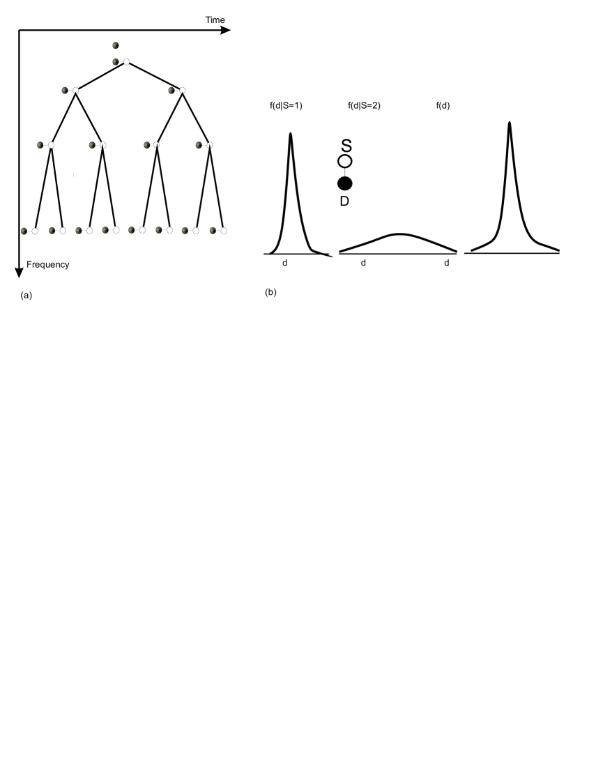
Figure 1: (a)Statistical model of the wavelet transform. Each coefficient $D_{i}$ (black node) is modeled as a mixture with the hidden state variable $S_{i}$ (white node). Hidden states are linked to each other vertically across scales to yield the Hidden Markov tree (HMT) model.(b)Gaussian two-state mixture model. The model is completely parametrized by the probability mass function (pmf) of the state variable, p_S(1), 1-p_S(1), and the means and the variances of the two Gaussian probability density functions (pdf’s). The Gaussian conditional pdf’s for D$|$S are at the left and the center, while the overall non-Gaussian pdf is on the right.

Due to the wavelet tree structure, each node at the coarser scale has two successors at the finer one that share its spatial support. As a consequence, appearance of yang (yin) coefficient in a node very likely means that its successors will be yang (yin) coefficients. For that reason, hidden states tend to propagate across scales (persistence property) crouse . Out of this dependency existing at the hidden state level, detail coefficients are considered to be decorrelated. Accordingly, dependencies in the wavelet tree can be completely modeled by conditional probabilities for parent-child hidden variable pairs. In that way, hidden variables obtain Markov tree structure which, together with (2), forms HMM for the wavelet tree crouse .

For $M$-state Gaussian mixture model for each wavelet coefficient (2), HMM is determined with parameter model vector

$${\mathbf{\theta}}=(p_{1}^{m},\epsilon_{i|i\neq 1}^{mn},\mu_{i}^{m},\sigma_{i}^{m}|i=1\dots I;m,n=1\dots M)$$ (3)

using abbreviations $p_{i}^{m}=P_{S_{i}}(m)$, $\epsilon_{i}^{mn}=P_{S_{i}|S_{\rho(i)}=m}(n).$ Parameter estimation is performed by applying the maximum likelihood principle (ML) which is asymptotically efficient, unbiased and consistent as the number of observations increases. Direct ML estimation of the model parameters (3) from the observed data is intractable since in estimating ${\mathbf{\theta}}$ we are characterizing the unobserved (hidden) states ${\mathbf{S}}=(S_{i}|i=1\dots I)$ of the wavelet coefficients $\mathbf{d}=(d_{i})$. Yet, given the values of the states, ML estimator of ${\mathbf{\theta}}$ is simple (merely ML estimator of Gaussian means and variances). Therefore, we employ an iterative expectation maximization (EM) approach dempster , which jointly estimates both the model parameters ${\mathbf{\theta}}$ and probabilities for the hidden states ${\mathbf{S}}$, given the observed coefficients $\mathbf{d}$.

Due to the limited data available usually from only one or few signal observations random variables that have similar properties are modeled using a common distribution or common parameter set, the practice is known as tying rabiner . In order to ensure reliable parameter estimation we must share statistical information between related wavelet coefficients so we assume that all wavelet coefficients and state variables within a common scale are identically distributed, including identical parent-child state transition probabilities. Consequently, in the following index $j$ in $p_{j}^{m}$, $\epsilon_{j}^{mn}$, $\mu_{j}^{m}$, $\sigma_{j}^{m}$ will denote the scale since all parameters of the particular scale are tied to the same value. The efficiency of the wavelet-domain HMM is demonstrated in crouse by developing a novel signal denoising method. Reconstructing the original signal all states with variances less then the noise variance are estimated to a single common value i.e. their informational content is completely lost.Having background noise of unknown power, all yin states of the data are essentially unreliable and suspected that their content is corrupted by noise. Thus, their content is certainly preserved only in nearby yang coefficients meaning that optimality of decomposition implies uniform distribution of yang coefficients in the wavelet tree.

A paradigmatic approach to the emergence of self-organization phenomena, presented in cosma1 , cosma2 and feldman begins with a dynamic random field on the network on which the random field of local causal states is constructed. To predict the original field either locally or globally, it is sufficient to know causal states. We find that this model shares common features with the wavelet-domain HMM and extend this analogy to a new level. The starting point in analyzing and predicting observations is to regard them as distorted measurements of another, unseen set of state variables which have their own dynamics. We comply with the framework of grassberger , where the complexity is the minimal amount of information about the system’s state needed for optimal prediction and further follow the idea of crutch0 to identify the complexity of a system with an amount of information needed to specify its causal state, the quantity labeled as statistical complexity. Following cosma1 and grassberger the local statistical complexity is defined as the entropy of local causal state

$$C(x,t)=H(S(x,t)).$$ (4)

If a spatially stationary process is dynamically autonomous from external influences self-organization takes place between time $t$ and time $t+T$ if and only if $C(x,t)<C(x,t+T)$ cosma1 . Our aim is to perceive HMM from the viewpoint of self-organization giving the concept of self-organization specific physical interpretation within the model. Some semantic analogies of the terms used in cosma1 and cosma2 and the wavelet-domain HMM will be used in order to make the ideas more clear. First, it is necessary to define the time axis. Interdependence of the nodes takes place vertically through the tree (persistence property) so we consider time axis as dyadic frequency axis directed from the coarsest to the finest scale. We regard signal domain as spatial even for temporal signals because the concept of time is replacing the frequency domain. Thus, by introducing diffeomorphism invariance the wavelet tree becomes the spatio-temporal tree. The direction of time is determined by the branching process representing information flow from parent to descendant coefficients. In the context of binary tree structure and the chosen time axis causality is defined by interdependence of the wavelet coefficients so it lies solely in the HM structure of the wavelet tree. Tying in the EM algorithm implies stationarity (and vice versa) in the spatial domain. Due to persistence property causality, considered as an optimal prediction of the wavelet tree containing information about yin and young states, is defined by presence or absence of singularity in the spatial support of wavelet coefficients. Therefore, hidden state variables $S_{i}$ are considered as local causal states which form the wavelet machine or w-machine in analogy with the $\epsilon-$ machine presented in crutch1 and crutch2 . Random variable $\mathbf{S}=(S_{i})$ represents the global causal state which contains minimal information for optimal prediction in the spatial domain. The proof follows from the EM algorithm which minimizes $H(\mathbf{S}|\mathbf{d})$ so we have $\mathbf{S}=f_{\theta}(\mathbf{D})$. Knowledge of $\mathbf{S}$ is related to optimal prediction because $\mathbf{D}$ in HMM depends on $\mathbf{S}$ only. The entropy of the wavelet tree may be expressed as

$$H(\mathbf{D})=H(\mathbf{D},\mathbf{S})=H(\mathbf{D}\left|\mathbf{S}\right)+H(\mathbf{S}),$$ (5)

where $H(\bf{D})$ and $H(\bf{D}\left|\bf{S}\right)$ are differential entropies of continuous random variables. The extensive term $H(\bf{D}\left|\bf{S}\right)$ represents irreducible randomness that remains even after all correlations are subsumed. Addition of noise increases only this term while complexity $H(\mathbf{S})$ remains unaltered. Local complexity $C_{i}=H(S_{i})$ has a specific physical interpretation - it is higher if the distribution of hidden yang an yin states in the node is more uniform. In that case, there is higher probability of yang coefficient appearance based on the persistence property in the nodes at the immediate neighboring scales meaning that information stored in $D_{i}$ will be preserved. Yet, it should be noted that local causal state in this model is statistic of the whole tree $\mathbf{D}$, thus separation into future and past becomes irrelevant for causality. Local causality implies both prediction and retrodiction and this property of the model we call temporal irrelevance. We indicated that local complexity $C_{i}=H(S_{i})$ is the measure which guarantees that the information contained in the node is optimally preserved. Global complexity $C=H({\mathbf{S}})$ fulfills that goal for the complete tree. Higher global complexity means that yang states are more uniformly distributed within the tree allowing for more optimal preservation of background information. So, we define optimal representation of the data (signal) as the one which maximizes global complexity of the tree. We note that factorization of global causal state into local ones in the wavelet HMM is different from the model presented in cosma1 because global state is not determined from local states in only one time instant. This is the consequence of temporal irrelevance since prediction takes into consideration the complete signal, i.e. both the past and the future of the wavelet tree. Regardless of these differences, we demonstrate that optimality of decomposition is related to the increase of local complexity and thus to the self-organization.

Derivation of the global complexity in terms of model parameters yields

$$C=H({\mathbf{S}})=\sum_{m}-p_{0}^{m}(logp_{0}^{m}+\sum_{n}2\epsilon_{1}^{mn}(log\epsilon_{1}^{mn}+\sum_{r}2\epsilon_{2}^{nr}(log\epsilon_{2}^{nr}+\dots)))$$ (6)

This expression takes higher values if conditional variables $S_{i}|S_{\rho(i)}=m$ are more uniformly distributed i.e. if probability of changing state is higher. But in this case local states also tend to be more uniformly distributed so that local complexity increases. It is also related to successful denoising using algorithm presented earlier, because higher complexity suggests more uniform distribution of yang coefficients and so information contained in the yin coefficients, which are more affected by noise, is preserved better. We have tested the model on a variety of signals and here we include the y-component of the Lorentz chaotic oscillator. White Gaussian noise of variance equal to 1 is added to the signal. The energy density of the remaining noise is estimated after denoising. Increase of local complexity in temporal domain is evaluated as maximal length of the interval at which the complexity function increases monotonically. In Table 1 we present results for the y-component of the Lorentz chaotic oscillator. The entropy is normalized so that it is bounded between 0 and 1. Representatives from the standard wavelet families are included, namely Haar (haar), Daubechies (db2), Symlet (sym3), Coiflet(coif1), Biorthogonal (bior1.3), Reverse Biorthogonal (rbior1.3) and Discrete Meyer (dmey). Biorthogonal wavelets are named as Biorn1.n2 where n1 is the number of the order of the wavelet or the scaling function and n2 is the order of the functions used for decomposition. Brief inspection of Table 1 suggests the discrete Meyer wavelet (dmey), marked in bold, as the optimal choice. It should be emphasized that energy density of the remaining noise is not an indicator of optimality of representation, because optimal representation is a general concept independent of particular signal processing application. However, it is obvious that optimality of representation based on self-organization in the wavelet-tree implies optimal wavelet-based noise reduction.

wavelet	haar	db2	sym3	coif1	bior1.3	rbio1.3	dmey
remaining noise	0.6138	0.3888	0.3234	0.3821	0.6442	0.3142	0.2559
global complexity	0.2984	0.6474	0.7300	0.6507	0.2350	0.6795	0.8075

   
Table 1.

We illustrate the method in the context of dynamical systems by considering structure and randomness of the time series generated by the logistic map on the unit interval $f(x)=rx(1-x)$, where $r\in[0,4]$. The term $H(\mathbf{S})$ in Eq.(5) represents the measure of complexity (structure) and the conditional entropy $H(\bf{D}\left|\bf{S}\right)$ is the measure of randomness. Both are represented in Fig. 2 as a function of parameter $r$ generated using the optimal, biorthogonal1.3, wavelet. The maximum complexity is attained for parameter value 3.5926, i.e. the value at which the deterministic chaos sets in. In Fig. 3 we present the complexity-entropy diagram corresponding to the $r\in[2.8,4]$ parameter region.

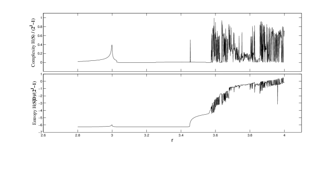
Figure 2: Complexity $H(S)/(2^{J}-1)$ and entropy rate $H(D|S)/(2^{J}-1)$ as a function of the parameter r. The r values were sampled uniformly in increments of 0.0001. Note the negative entropy values as a consequence of the differential entropy property.

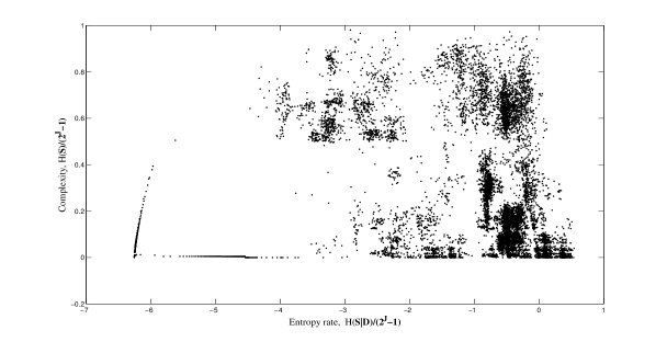
Figure 3: Entropy rate and complexity pairs $(H(D|S)/(2^{J}-1),H(S)/(2^{J}-1))$ for the logisitic map. The parameter $r$ values were sampled uniformly in increments of $0.0001$. Negative entropy values stem from the properties of differential entropy that takes all values from $\mathbb{R.}$

For a given value of entropy multiple values of complexity are noticed indicating an intricate relationship between these two quantities. Not all complexity values are realizable for a particular entropy rate. Organization is evident in the diagram consisting of low and very high density regions exhibiting self-similar structure in the central part of the diagram. Both the lower and the upper bounds are well defined.

We have argued that w-machine establishes relationship between information, prediction, retrodiction and denoising founded on the choice of the optimal wavelet and within the framework of statistical mechanics. Statistical complexity may be reliably calculated from data and at the same time noise may be removed in a highly efficient manner. The method can be easily adapted to 2-dimensional signals.

The authors acknowledge support by the Serbian Ministry of Education and Science through the projects OI 174014 and III 44006.

References

- (1) Eugenio Hernandez, Guido Weiss A First Course on Wavelets, CRC PRESS, Boca Raton, 1996.
- (2) Stephane Mallat, A Wavelet Tour of Signal Processing, The Sparse Way, Elsevier, Amsterdam 2009.
- (3) O. Pont, A. Turiel and C.J. Pérez-Vicente, Journal of Wavelets, Multiresolution and Information Processing 9, 35 (2011).
- (4) O. Pont, A. Turiel and C.J. Pérez-Vicente, Phys. Rev. E 74, 061110 (2006).
- (5) M. Crouse, R. Nowak, R. Baraniuk, IEEE Transactions on Signal Processing 46, 886 (1998).
- (6) A.P.Dempster, N.M.Laird, D.B.Rubin, J.R. Stat. Soc. 39, 1 (1977).
- (7) L.Rabiner, Proc. IEEE 77, 257 (1989).
- (8) C. R. Shalizi, Discrete Math. Theor. Comput. Sci. 11 (2003).
- (9) C. R. Shalizi, K. L. Shalizi, R. Haslinger, Phys. Rev. Lett. 93, 118701 (2004).
- (10) P. Grassberger, Int. J. of Theor. Phys. 25, 907 (1996).
- (11) J. P. Crutchfield, K. Young, Phys. Rev. Lett. 63, 105 (1989).
- (12) N. F. Travers and J. P. Crutchfield, J. Stat. Phys. 145, 1181 (2011).
- (13) N. F. Travers and J. P. Crutchfield, J. Stat. Phys. 145, 1202 (2011).
- (14) D.P. Feldman, C.S. McTague, and J.P. Crutchfield, Chaos, 18, 043106. (2008).