Entanglement measures and the quantum to classical mapping

Abstract

A quantum model can be mapped to a classical model in one higher dimension. Here we introduce a finite-temperature correlation measure based on a reduced density matrix $\bar{\rho}_{\bar{A}}$ obtained by cutting the classical system along the imaginary time (inverse temperature) axis. We show that the von-Neumann entropy $\bar{S}_{\rm ent}$ of $\bar{\rho}_{\bar{A}}$ shares many properties with the mutual information, yet is based on a simpler geometry and is thus easier to calculate. For one-dimensional quantum systems in the thermodynamic limit we proof that $\bar{S}_{\rm ent}$ is non-extensive for all temperatures $T$. For the integrable transverse Ising and $XXZ$ models we demonstrate that the entanglement spectra of $\bar{\rho}_{\bar{A}}$ in the limit $T\to 0$ are described by free-fermion Hamiltonians and reduce to those of the regular reduced density matrix $\rho_{A}$—obtained by a spatial instead of an imaginary-time cut—up to degeneracies.

Entanglement is usually thought of as a quantum mechanical entity yet it is well known that the properties of quantum models can be computed from a classical model in one dimension higher Suzuki (1976); Zinn-Justin (1989); Sachdev (1999). Such an approach is particularly useful if one is interested in how entanglement builds up in a thermal state while lowering the temperature or during unitary time evolution.

Entanglement measures are, generally speaking, maps from the space of density matrices into the positive real numbers. Various entanglement measures have been introduced in the last decades and a set of axioms has been put forward which a good measure should possess Vedral et al. (1997); Plenio and Virmani (2007). For bipartite pure states the von-Neumann entropy of entanglement fulfills these criteria and provides a bridge into statistical mechanics and condensed matter physics. In particular, the reduced density matrix, whose eigenvalues determine the entanglement entropy, is at the heart of the density matrix renormalization group (DMRG) White (1992). This numerical method allows one to optimally approximate pure states of many-body systems by matrix product states Östlund and Rommer (1995) and is most successful in one dimension.

In experiments we are, however, usually dealing with mixed states about whose entanglement properties much less is known. Entanglement measures commonly used for pure states of multi-particle systems such as the entanglement entropy fail because they become extensive and thus no longer fulfill a boundary law. Furthermore, they cannot distinguish between classical and quantum correlations Vedral et al. (1997). Entanglement measures which do distinguish between these different types of correlations involve extremizations over all possible decompositions of the density matrix and explicit results have only been obtained for few-particle density matrices Wootters (1998); Arnesen et al. (2001); Dillenschneider (2008). Putting these fundamental difficulties aside, it is still useful to define correlation measures for thermal ensembles which go beyond the one- and two-point correlation functions traditionally studied in statistical mechanics and condensed matter physics. They might help to reveal, in particular, phase transitions with complex or topological order parameters.

In this letter we want to investigate how correlations, generated during imaginary time evolution, can be quantified. After a quantum to classical mapping we introduce as entanglement measure the von-Neumann entropy of a reduced density matrix obtained by a partial trace in the imaginary time direction. This measure also cannot distinguish between quantum and classical correlations but we will show that it shares many properties with the mutual information which has recently attracted considerable interest as a correlation witness for many-body systems Isakov et al. (2011); Singh et al. (2011); Wilms et al. (2012, 2011). The measure introduced in this letter is also a natural choice from the perspective of numerical matrix product state algorithms: While the reduced density matrix obtained by a spatial trace is at the heart of the DMRG at $T=0$, the reduced density matrix considered here is used in transfer-matrix DMRG algorithms to study the finite-temperature properties of one-dimensional systems in the thermodynamic limit Bursill et al. (1996); Wang and Xiang (1997); Shibata (1997); Sirker and Klümper (2002); Sirker (2010).

The entanglement entropy for a bipartite system, $S=A\cup B$, is defined as

$$S_{\rm ent}(A)=-\operatorname{Tr}\rho_{A}\ln\rho_{A}$$ (1)

where $\rho_{A}=\operatorname{Tr}_{B}\rho$, $\operatorname{Tr}\rho_{A}=1$, is a reduced density matrix obtained from the density matrix $\rho$ of the system $S$ by spatially tracing out part $B$. If the system is in a pure state, then it is easy to show by a Schmidt decomposition that $S_{\rm ent}\equiv S_{\rm ent}(A)=S_{\rm ent}(B)$. It follows that $S_{\rm ent}$ cannot be extensive but rather has to scale with the surface between regions $A$ and $B$ Srednicki (1993). In critical one-dimensional systems this boundary law is known to be weakly violated by logarithmic corrections Holzhey et al. (1994); Calabrese and Cardy (2004). Here we want to study the mixed state described by the canonical density matrix $\rho_{\rm c}=\exp(-\beta H)/Z$ where $\beta$ is the inverse temperature, $H$ the Hamiltonian, and $Z=\operatorname{Tr}\rho_{\rm c}$ the partition function. Calculating the entanglement entropy (1) for $\rho_{c}$ one finds that $S_{\rm ent}(A)\neq S_{\rm ent}(B)$ in general and that $S_{\rm ent}$ becomes an extensive quantity approaching the regular thermal von-Neumann entropy for $\beta\to 0$ Calabrese and Cardy (2004); Sorensen et al. (2007). This can be easily understood as follows: If all correlation lengths are much smaller than the extent of the considered subsystem then the rest of the system just acts as an additional bath. A way to partly correct this is to consider the mutual information given by $\mathcal{I}_{A,B}=S_{\rm ent}(A)+S_{\rm ent}(B)-S_{\rm th}(A\cup B)$ where $S_{\rm th}(A\cup B)=-\operatorname{Tr}\rho_{c}\ln\rho_{c}$ is the von-Neumann entropy of the whole system. The thermal contribution is then explicitly subtracted ensuring that $\mathcal{I}_{A,B}(\beta\to 0)\to 0$ as required. However, the mutual information is still not a proper entanglement measure because classical as well as quantum correlations contribute. Furthermore, the evaluation of the mutual information even when using Renyi instead of von-Neumann entropies is quite involved due to the complicated geometry required to obtain generalized partition functions Calabrese and Cardy (2004); Melko et al. (2010); Isakov et al. (2011); Singh et al. (2011); Wilms et al. (2011). An obvious question is if related finite-temperature correlation measures can be defined which are easier to use in analytical and numerical calculations.

Coupled qubits

To motivate the idea of a correlation measure based on a quantum-to-classical mapping we start with two coupled qubits with Hamiltonian $H=\boldsymbol{S}_{1}\cdot\boldsymbol{S}_{2}$ where $\boldsymbol{S}$ is a spin-$1/2$ operator. Let us consider first the imaginary time evolution starting from the separable state $\mid\uparrow\downarrow\rangle=(\mid\uparrow\downarrow\rangle+\mid\downarrow\uparrow\rangle)/2+(\mid\uparrow\downarrow\rangle-\mid\downarrow\uparrow\rangle)/2$. Time evolving with $\text{e}^{-\beta H}$ this state becomes $|\Psi_{\beta}\rangle=\frac{\exp(-\beta/4)}{2}(\mid\uparrow\downarrow\rangle+\mid\downarrow\uparrow\rangle)+\frac{\exp(3\beta/4)}{2}(\mid\uparrow\downarrow\rangle-\mid\downarrow\uparrow\rangle)$ and gets projected onto the maximally entangled singlet ground state for $\beta\to\infty$. A picture showing how the entangled state is formed out of the separable state can be obtained by the quantum-to-classical mapping. We discretize time into steps $\delta\beta$ writing $\rho_{\rm c}=\tau^{M}/Z$ where $\tau=\exp(-\delta\beta\,H)$ and $M\delta\beta=\beta$. Rewriting the Hamiltonian as $H=\frac{1}{2}P_{1,2}-\frac{1}{4}\mbox{Id}_{1,2}$ we find

$$\tau\approx(1+\frac{\delta\beta}{4})\mbox{Id}_{1,2}-\frac{\delta\beta}{2}P_{1,2}$$ (2)

where $\mbox{Id}_{1,2}$ is the identity and $P_{1,2}$ the operator permuting the spins at sites $1,2$ during the time step $\delta\beta$. Entanglement is thus being generated during imaginary time evolution by the braiding of the worldlines of the two spins. This is shown pictorially for one possible configuration of $\tau$-matrices in Fig. 1(a). For the separable initial state $\mid\uparrow\downarrow\rangle$, the correlations created can be measured by $S_{\rm ent}$, Eq. (1), using $\rho=|\Psi_{\beta}\rangle\langle\Psi_{\beta}|/\langle\Psi_{\beta}|\Psi_{\beta}\rangle$ as density matrix and tracing out one of the spins (see Fig. 1(e)). When using $\rho_{\rm c}$ as the density matrix , on the other hand, one finds $S_{\rm ent}=\ln 2$ independent of temperature. Thus $S_{\rm ent}$ fails as a correlation measure and the whole temperature dependence of the mutual information, see Fig. 1(e), stems from the thermal von-Neumann entropy with $\mathcal{I}_{A,B}\sim 3/32T^{2}$ for $T\to\infty$.

Here we want to pursue a different perspective on the classical representation of the qubits shown in Fig. 1(b) by defining a transfer matrix operator, a method often used in statistical mechanics.

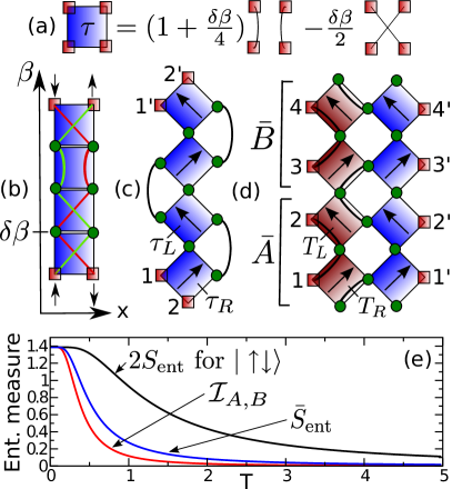
Figure 1: (Color online) (a) Local Boltzmann weight $\tau$, Eq. (2). (b) Braiding of worldlines during imaginary time evolution discretized in steps $\delta\beta$ with green circles denoting tensor contractions. (c) Density matrix $\rho_{c}(1,2|1^{\prime},2^{\prime})$, the lines connect contracted indices. (d) Density matrix $\bar{\rho}(1,2,3,4|1^{\prime},2^{\prime},3^{\prime},4^{\prime})$ projecting onto the ground state in auxiliary space. (e) Entanglement measures as function of temperature.

One way to achieve this is to perform an alternating $45^{\circ}$ clockwise and anti-clockwise rotation of the $\tau$-plaquettes starting from Fig. 1(b). This leads to the completely equivalent graphical representation shown in Fig. 1(c) with plaquettes $\tau_{R,L}=T_{R,L}\tau$ where $T_{R,L}$ is the right/left shift operator, respectively. Tracing either over the pair of open indices $1,1^{\prime}$ or $2,2^{\prime}$ gives the reduced density matrix $\rho_{A}$ while tracing over both pairs gives the partition function $Z$. By moving the right $\delta$ bonds (lines in Fig. 1(c)) to the left and tracing over $1,1^{\prime}$ and $2,2^{\prime}$ we obtain the density matrix $\bar{\rho}$ acting in auxiliary space along the imaginary time axis. $\bar{\rho}$, shown in Fig. 1(d), consists of two columns with the left column containing only right and left shift operators, $T_{R,L}$. Contracting pairwise the open indices $1,\cdots,4$ on the left side with $1^{\prime},\cdots,4^{\prime}$ on the right side yields again $Z$. We now investigate the reduced density matrix $\bar{\rho}_{\bar{A}}=\mbox{Tr}_{\bar{B}}\bar{\rho}$ obtained by taking a partial trace in auxiliary space. $\bar{\rho}_{\bar{A}}$ is then a $4\times 4$ matrix whose eigenvalues can be easily calculated. Note that regions $\bar{A},\bar{B}$ always have to contain an even number of $\tau_{R,L}$-plaquettes so that the number of right and left shift operators is the same. A discretization using more than four plaquettes would, in the simple case considered, just add additional zero eigenvalues. The entanglement measure $\bar{S}_{\rm ent}(\bar{A})=-\operatorname{Tr}\bar{\rho}_{\bar{A}}\ln\bar{\rho}_{\bar{A}}=\bar{S}_{\rm ent}(\bar{B})$ is thus well-defined with $\lim_{T\to 0}\bar{S}_{\rm ent}=2\ln 2$ and $\bar{S}_{\rm ent}\sim 3(1+6\ln 2+2\ln T)/64T^{2}$ for $T\to\infty$, see Fig. 1(e).

Next, we want to generalize these considerations to one-dimensional quantum systems. A Hamiltonian with short-range interactions can always be written as $H=\sum_{j}h_{j,j+1}$, possibly in an enlarged unit cell. By using a Trotter-Suzuki decomposition, the system can be mapped onto a two-dimensional classical system in much the same way we have mapped the qubits onto a one-dimensional classical system. A pictorial representation is shown in Fig. 2(a) where each plaquette is given by $\tau_{R,L}=T_{R,L}\exp(-\delta\beta h_{j,j+1})$.

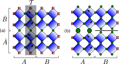
Figure 2: (Color online) (a) Two-dimensional lattice obtained after the quantum-to-classical mapping. The shaded part is the QTM $\mathcal{T}$. Performing the trace over $\bar{A}$, $\bar{B}$ and the partial spatial trace over region $B$ yields $\rho_{A}$ while tracing over $A,B$ and taking the partial trace over region $\bar{B}$ yields $\bar{\rho}_{\bar{A}}$. (b) Geometry to calculate $\operatorname{Tr}\rho_{A}^{2}$. The right part consists of two small cylinders while the left part is one big cylinder.

Note that $[h_{j,j+1},h_{k,k+1}]\neq 0$ in general so that the mapping induces an error which is of order $(\delta\beta)^{2}$ for the partition function.

The canonical density matrix $\rho_{\rm c}$ for periodic boundary conditions is shown pictorially in Fig. 2(a) with the l.h.s. and r.h.s. indices traced over. Tracing instead over the upper and lower indices and leaving the indices on the l.h.s. and r.h.s. open we obtain the density matrix $\bar{\rho}=\mathcal{T}^{L}/Z$ where $\mathcal{T}$ is a quantum transfer matrix (QTM) acting in auxiliary space. The partition function is given by $Z=\operatorname{Tr}_{A,B}\rho_{c}=\operatorname{Tr}_{\bar{A},\bar{B}}\bar{\rho}$. For any $T>0$ the thermodynamic limit can now be performed exactly with $\lim_{L\to\infty}\bar{\rho}=|\Psi_{R}\rangle\langle\Psi_{L}|$. Here $|\Psi_{R}\rangle$ and $\langle\Psi_{L}|$ are the left and right eigenvectors belonging to the largest eigenvalue of $\mathcal{T}$ with $\langle\Psi_{L}|\Psi_{R}\rangle=1$. This property can be easily understood physically because all correlation lengths—determined by the logarithm of the ratio of the leading to subleading eigenvalues of $\mathcal{T}$—stay finite. $\bar{\rho}$ thus becomes a projector onto the ground state in auxiliary space. Note that in this representation $\bar{\rho}$ is non-symmetric. A symmetric representation is also possible but would require a wider column transfer matrix $\mathcal{T}$. The reduced density matrix $\bar{\rho}_{\bar{A}}=\operatorname{Tr}_{\bar{B}}\bar{\rho}$ is then obtained by tracing over half of the indices along the imaginary time axis. Crucially, it is again easy to show using a Schmidt decomposition and choosing biorthonormal sets of right and left basis vectors that $\bar{S}_{\rm ent}\equiv\bar{S}_{\rm ent}(\bar{A})=\bar{S}_{\rm ent}(\bar{B})$. $\bar{\rho}$ being a projector thus guarantees that $\bar{S}_{\rm ent}$ is non-extensive for all temperatures $T$. It is thus quite natural to replace the projector $\rho$ onto the ground state, considered for zero temperature, with the projector in auxiliary space, $\bar{\rho}$, for an infinite one-dimensional system at finite temperatures.

Because $\rho_{A}$ is not a projector for $T>0$, $S_{\rm ent}(T)$ is difficult to calculate. Instead, the replica trick is often used Calabrese and Cardy (2004) which leads to the definition of Renyi entropies $S_{n}(A)=\ln[\operatorname{Tr}(\rho^{n}_{A})]/(1-n)$. A quantum-to-classical mapping yields the geometry for $\operatorname{Tr}(\rho^{2}_{A})$ shown in Fig. 2(b). Separate QTM’s for the right and left part of the system can then be defined, however, an evaluation of $S_{2}(A)$ requires one to calculate overlaps between the eigenstates of the QTM’s Wilms et al. (2011) and is thus much harder than obtaining $\bar{S}_{\rm ent}$. In the following, we study in more detail the scaling properties of $\bar{S}_{\rm ent}(T)$ and the spectra of $\bar{\rho}_{\bar{A}}$ for a symmetric cut $\bar{A}=\bar{B}=\beta/2$.

Transverse Ising model

We start with the transverse Ising model

$$H=\sum_{j}\left(\sigma^{z}_{j}\sigma^{z}_{j+1}+\lambda\sigma^{x}_{j}\right)$$ (3)

where $\boldsymbol{\sigma}$ are the Pauli matrices. This model shows a second order phase transition at $\lambda=1$ Sachdev (1999). To study $\bar{S}_{\rm ent}(T)$ and the entanglement spectra of $\bar{\rho}_{\bar{A}}$ we use a transfer matrix renormalization group (TMRG) algorithm Bursill et al. (1996); Wang and Xiang (1997); Shibata (1997); Sirker and Klümper (2002).

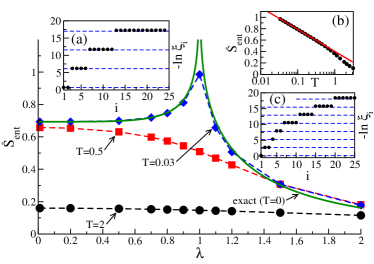
Figure 3: (Color online) TMRG results are denoted by symbols. Main: $\bar{S}_{\rm ent}$ for various $T$ and exact result for $T=0$ (solid line). Eigenvalues $\xi_{i}$ of $\bar{\rho}_{\bar{A}}$ for (a) $\lambda=0.8$ and (c) $\lambda=1.2$ at $T=0.02$. The free fermion levels are denoted by dashed lines. (b) $\bar{S}_{\rm ent}(T)$ for $\lambda=1$ and low-temperature fit $S_{\rm ent}=-0.167\ln T+0.402$.

The entanglement spectra in the low-temperature limit are shown exemplarily in Fig. 3(a,b) and are equally spaced. The degeneracies of the dominant eigenvalues are given by $2,4,6,12,\cdots$ for $\lambda<1$ and $1,2,1,2,4,4,5,6,\cdots$ for $\lambda>1$. As for the reduced density matrix $\rho_{A}$ obtained by a spatial cut Peschel et al. (1999) these spectra can be explained by using corner transfer matrices (CTM’s). We find $\bar{\rho}_{\bar{A}}=\text{e}^{-H_{CTM}}/\operatorname{Tr}\text{e}^{-H_{CTM}}$ where $H_{CTM}=\sum\epsilon_{j}n_{j}$ is a free fermion Hamilton operator. For $\lambda>1$ all single particle levels are twofold degenerate, $n_{j}=0,1,2$, and given by $\epsilon_{j}=(2j+1)\pi K(\sqrt{1-1/\lambda^{2}})/K(1/\lambda)$ where $K(x)$ is the complete elliptic integral of the first kind. For $\lambda<1$ we have $\epsilon_{j}=j\pi K(\sqrt{1-\lambda^{2}})/K(\lambda)$ where $\epsilon_{0}$ is non-degenerate and all other levels twofold degenerate. Knowing the spectrum in the zero temperature limit it is easy to calculate $\bar{S}_{\rm ent}(T\to 0)$ Calabrese and Cardy (2004). The result is shown as solid line in Fig. 3. Right at the critical point the regular entanglement entropy for an interval of length $\ell$ in an infinite chain shows a logarithmic divergence with system size, $S_{\rm ent}=\frac{c}{3}\ln\ell+C_{1}$, with central charge $c=1/2$ and a non-universal constant $C_{1}$ Calabrese and Cardy (2004). From this result it follows immediately by a conformal mapping that

$$\bar{S}_{\rm ent}(T)=\frac{c}{3}\ln(v/T)+C_{1}$$ (4)

with $v$ being the velocity of the elementary excitations. This result is universal for critical systems. For the transverse Ising model it is in excellent agreement with a two-parameter fit of the numerical data, see Fig. 3(b).

$XXZ$ model and boundary locality

As a further example, we calculate $\bar{S}_{\rm ent}$ and $\bar{\rho}_{\bar{A}}$ for the $XXZ$ model

$$H=J\sum_{j}\left\{S^{x}_{j}S^{x}_{j+1}+S^{y}_{j}S^{y}_{j+1}+\Delta S^{z}_{j}S^{z}_{j+1}\right\}\,.$$ (5)

Here $\boldsymbol{S}$ is a spin-$1/2$ operator and $\Delta$ parametrizes the exchange anisotropy. The model is critical for $-1<\Delta\leq 1$ with central charge $c=1$. As shown in Fig. 4 for three different values of $\Delta$, Eq. (4) does indeed describe $\bar{S}_{\rm ent}$ for $T\ll J$.

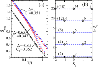
Figure 4: (Color online) (a) One-parameter fits (lines) for $T/J\leq 0.1$ of TMRG data (symbols) according to (4) with $c=1$, $v$ as known from the Bethe ansatz, and $C_{1}$ as indicated. (b) Spectrum of $\bar{\rho}_{\bar{A}}$ for $\Delta=10$ and $T/J=0.02$. The numbers give the multiplicities of each level (total in brackets), the dashed lines mark the free fermion levels.

The spectrum of $\rho_{A}$ in the non-critical case $\Delta>1$ can be constructed from a free-fermion Hamiltonian Peschel et al. (1999) and we find again that the same is also true for $\bar{\rho}_{\bar{A}}$ at low temperatures. As an example, the spectrum for $\Delta=10$ is shown in 4(b). The degeneracies of the free Fermion levels are the same as for the transverse Ising model with $\lambda<1$, however, now $\epsilon_{j}=2j\cosh^{-1}\Delta$ Peschel et al. (1999). $S^{z}_{\rm tot}=\sum_{j}S^{z}_{j}$ commutes with the Hamiltonian and is thus a good quantum number. For the QTM $\mathcal{T}$ it follows that $\bar{S}^{z}_{\rm R,L}=\sum_{k}(-1)^{k}\bar{(}S_{k}^{z})_{R,L}$ is a good quantum number where $(\bar{S}_{k}^{z})_{R,L}$ acts at site $k$ in auxiliary space on the r.h.s. respectively l.h.s. of $\mathcal{T}$. Matrix elements of $\mathcal{T}$ can thus only be non-zero if $\bar{S}^{z}\equiv\bar{S}^{z}_{\rm R}=\bar{S}^{z}_{\rm L}$ and eigenvalues of $\bar{\rho}_{\bar{A}}$ can be classified according to $\bar{S}^{z}$, see Fig. 4(b). For $\rho_{A}$ it has been shown that its spectrum as a function of $S^{z}_{\rm tot}$ can be constructed for $\Delta\gg 1$ by local perturbation theory in the spin exchange operator Alba et al. (2012). The same local perturbation theory can also be performed for the QTM $\mathcal{T}$. Keeping in mind that we have periodic boundary conditions along the imaginary time direction so that the partial trace introduces two boundaries, the degeneracies of each level for $\bar{\rho}_{\bar{A}}$ as a function of $\bar{S}^{z}$ are exactly the same as for $\rho_{A}$ with two boundaries classified by $S^{z}_{\rm tot}$. This demonstrates explicitly that a boundary law also holds for $\bar{\rho}_{\bar{A}}$ obtained by a cut along the imaginary time direction.

Ladders and two-dimensional models

The quantum-to-classical mapping of a finite two-dimensional system of extent $L_{1}\times L_{2}$ leads to a three-dimensional system with dimensions $\beta\times L_{1}\times L_{2}$. In order to calculate the mutual information $\mathcal{I}_{A,B}$ following a spatial cut one can again use the replica trick. In particular, the Renyi entropy $S_{2}$ has been obtained from the three-dimensional generalization of the geometry shown in Fig. 2(b) by quantum Monte Carlo (QMC) simulations Melko et al. (2010); Isakov et al. (2011); Singh et al. (2011). However, the non-trivial geometry makes these calculations rather complicated and $S_{\rm ent}$ remains inaccessible. On the contrary, the numerical calculation of $\bar{S}_{\rm ent}$ is straightforward also in two dimensions. For $L_{1}$ and $L_{2}$ both finite, one can use the mutual information $\bar{\mathcal{I}}_{\bar{A},\bar{B}}=\bar{S}_{\rm ent}(\bar{A})+\bar{S}_{\rm ent}(\bar{B})+\operatorname{Tr}\bar{\rho}\ln\bar{\rho}$ to detect finite temperature phase transitions. Furthermore, one can perform the thermodynamic limit in one of the spatial dimensions with $\lim_{L_{1}\to\infty}\bar{\rho}(L_{1},L_{2},\beta)=|\Psi_{R}\rangle\langle\Psi_{L}|$ becoming again a projector so that $\lim_{T\to\infty}\bar{S}_{\rm ent}=0$ and a subtraction of a ’thermal part’ is no longer required.

Discussion

We have analyzed the entanglement entropy $\bar{S}_{\rm ent}$ of a reduced density matrix obtained after a quantum-to-classical mapping and a partial trace in imaginary time direction. Our results show that transfer matrix DMRG algorithms are as efficient in simulating one-dimensional quantum systems in the thermodynamic limit at finite temperatures as regular DMRG algorithms are for finite systems at $T=0$. For two- and three-dimensional systems $\bar{S}_{\rm ent}$ can be used to investigate finite temperature phase transitions. For QMC, in particular, this might be a viable and—due to the simpler geometry—easier approach than calculating Renyi entropies.