A comparison between the stellar and dynamical masses of six globular clusters

Abstract

We present the results of a comprehensive analysis of the structure and kinematics of six Galactic globular clusters. By comparing the results of the most extensive photometric and kinematical surveys available to date with suited dynamical models, we determine the stellar and dynamical masses of these stellar systems taking into account for the effect of mass segregation, anisotropy and unresolved binaries. We show that the stellar masses of these clusters are on average smaller than those predicted by canonical integrated stellar evolution models because of the shallower slope of their mass functions. The derived stellar masses are found to be also systematically smaller than the dynamical masses by $\sim$ 40%, although the presence of systematics affecting our estimates cannot be excluded. If confirmed, this evidence can be linked to an increased fraction of retained dark remnants or to the presence of a modest amount of dark matter.

1. Introduction

Among the stellar system zoo there is a widely recognized discrepancy between the photon-emitting mass (constituted by stars and gas) and dynamical mass (including the contribution of dark matter). From galaxy clusters to dwarf galaxies the mass of the baryonic component, estimated through the conversion of light in mass, has been found to be significantly smaller than that estimated via kinematical considerations (see Tollerud et al. 2011 for a recent review). The commonly accepted solution to this problem invokes the presence of a large amount of dark, non-baryonic matter driving the kinematics of these systems without contributing to their luminosity. Within this framework, globular clusters (GCs) are considered a notable exception: although they are the next step down from the smallest stellar systems containing dark matter (the Ultra Compact Dwarf galaxies; Mieske et al. 2008) and brighter than the most dark matter dominated systems (the Ultra Faint Galaxies; Simon et al. 2011) they are not believed to contain dark matter (Baumgardt et al. 2009). This conclusion is mainly justified by the evidence that dynamical mass-to-light (M/L) ratios of GCs are $\sim$25% smaller than those predicted by simple stellar population models that assume a canonical Initial Mass Function (IMF; McLaughlin & van der Marel 2005; Strader et al. 2009, 2011). However, these models do not account for dynamical effects such as the preferential loss of low-mass stars due to energy equipartition which alters the shape of the present-day mass function (PDMF) and consequently the stellar M/L ratio. In fact, all the past determinations of PDMFs in GCs derived slopes shallower than that of a canonical (e.g. Kroupa 2001) IMF (Piotto & Zoccali 1999; Paust et al. 2010; De Marchi et al. 2010). In a recent paper Kruijssen & Mieske (2009) modeled the evolution of the mass function of 24 GCs including the effects of dynamical dissolution, low-mass star depletion, stellar evolution and stellar remnants finding a substantial agreement between the prediction of their model and the dynamical M/L ratio estimated through the cluster kinematics. They conclude that dynamical effects are likely responsible for the observed discrepancy between stellar and dynamical masses. The flood of available data from deep photometric and spectroscopic surveys make now possible to test this issue observationally at an higher level, sampling the mass function of GCs down to the hydrogen burning limit (Paust et al. 2010) and their velocity dispersion profile up to many half-mass radii (Lane et al. 2010a). This gives the unprecedented opportunity to derive stellar masses from direct star counts instead of converting light in mass, obtaining an estimate which does not require the assumption of a $M/L$ ratio.

In this paper we compare the results of deep Hubble Space Telescope (HST) photometric observations and wide-field radial velocities available from recent public surveys with a set of dynamical models with the aim of deriving the amount of stellar and dynamical mass in a sample of six Galactic GCs.

2. Observational material

For the present analysis we make use of three different databases:

• The set of publicy available deep ACS@HST photometric catalogs of the ”globular cluster treasury project” (Sarajedini et al. 2007);

• The radial velocities obtained by the AAOmega@AAT survey of GCs (Lane et al. 2011);

• The surface brightness profiles derived by Trager et al. (1995).

The photometric database consists of high-resolution HST observations of a sample of 65 Galactic GCs. The database has been constructed using deep images secured with the Advanced Camera for Surveys (ACS) Wide Field Channel through the F606W and F814W filters. The field of view of the camera ($202\arcsec\times 202\arcsec$) is centered on the clusters center with a dithering pattern to cover the gap between the two chips, allowing a full coverage of the core of all the six GCs considered in our analysis. This survey provides deep color-magnitude diagrams (CMD) reaching the faint Main Sequence (MS) of the target clusters down to the hydrogen burning limit (at $M_{V}\leq 10.7$) with a signal-to-noise ratio $S/N>10$. The results of artificial star experiments are also available to allow an accurate estimate of the completeness level and photometric errors. A detailed description of the photometric reduction, astrometry and artificial star experiments can be found in Anderson et al. (2008). Since all the considered GCs have relaxation times shorter than their ages (Mc Laughlin & van der Marel 2005), the effects of mass segregation are expected to be important. It is therefore useful to constraint the radial variation of the MF outside the half-mass radius. Unfortunately, the ACS treasury survey covers only the central part of the cluster at distances $<2\arcmin$ from the cluster centers. Additional deep data sampling the external part of the cluster are available only for NGC288. They consist of a set of ACS images observed under the program GO-12193 which are centered at $\sim 5\arcmin$ away from the cluster center. In particular, $3\times 200~{}s$ + $1\times 15~{}s$ long exposures have been taken through the F606W filter and $3\times 150~{}s$ + $1\times 10~{}s$ long exposures through the F814W one. All images were passed through the standard ACS/WFC reduction pipeline. Data reduction has been performed on the individual pre-reduced (.flt) images using the SExtractor photometric package (Bertin & Arnouts 1996). For each star we measured the flux contained within a radius of 0.1 arcsec (corresponding to 2 pixel $\sim$FWHM) from the star center. We preformed the source detection on the stack of all images while the photometric analysis has been performed independently on each image. Only stars detected in two out of three long-exposures or in the short ones have been included in the final catalogue. We used the most isolated and brightest stars in the field to link the aperture magnitudes at 0.5 arcsec to the instrumental ones, after normalizing for exposure time. Instrumental magnitudes have been transformed into the VEGAMAG system by using the photometric zero-points by Sirianni et al. (2005). Finally, each ACS pointing has been corrected for geometric distortion using the prescriptions by Hack & Cox (2001). We preformed artificial star experiments on the science frames following the prescriptions described in Sollima et al. (2007). In summary, a set of artificial stars have been simulated using the Tiny Tim model of the ACS PSF (Krist et al. 2010) and added to all images at random positions within $36\times 36$px cells centered on a grid of $100\times 50$ knots along the x and y directions of the two ACS chips (a single star for each cell). The F814W magnitude of each star has been extracted from a luminosity function simulated adopting a Kroupa (2001) mass function which has been converted in F814W magnitude using the mass-luminosity relation of Dotter et al. (2007). The corresponding F606W magnitude has been derived by interpolating along the cluster mean ridge line of the F814W-(F606W-F814W) CMD. We performed the photometric reduction on the simulated frames with the same procedure adopted for the science frames producing a catalog of $\sim 10^{5}$ artificial stars.

The radial velocity database has been derived by Lane et al. (2009, 2010a, 2010b, 2011) from a large number of spectra of Red Giant Branch (RGB) stars observed in fields centered on 10 Galactic GCs. Spectra were obtained with the multi-fiber AAOmega spectrograph mounted at the Anglo Australian Telescope with the 1700D and the 1500V gratings on the red and blue arm, respectively. With this configuration spectra covering the Ca II triplet region (8340-8840 Å) and the swathe of iron and magnesium lines around $\sim 5200$Å were obtained with a resolution of R=10000 and R=3700 for the red and blue arms, respectively. A detailed description of the reduction procedure and radial velocities estimates can be found in Lane et al. (2009, 2010a, 2010b, 2011). For the present work we adopted the radial velocities extracted with the RAVE pipeline since they provide a better estimate of the radial velocity uncertainty when compared with the available high-resolution spectroscopic studies (see Bellazzini et al. 2012). In the analysis we used only stars satisfying the same membership criterion adopted by these authors and within $d<2~{}r_{h}$ from the cluster center (see Sect. 4); they are 132 in NGC288, 164 in NGC5024, 190 in NGC6218, 357 in NGC6752, 676 in NGC6809 and 193 in NGC7099.

The surface brightness profiles were taken from the Trager et al. (1995) database. They were constructed from generally inhomogeneous data based mainly on the Berkeley Globular Cluster Survey (Djorgovski & King 1984). The surface brightness profile of each cluster has been derived by matching several set of data obtained with different techniques (aperture photometry on CCD images and photographic plates, photoelectric observations, star counts, etc.). Although these inhomogeneities may represent a drawback of the analysis (see Sect. 6.1), this database represents the unique collection of wide field surface brightness profiles covering the entire extent of the target clusters up to their tidal radius.

The target clusters analyzed in this work were selected among the 10 objects in common between the three above databases requiring that i) the photometric observations reach the magnitude of stars with masses $M\sim 0.15~{}M_{\odot}$ with a completeness level $\geq 50\%$, and ii) the systemic rotation does not exceed the 10% of the cluster velocity dispersion. This last requirement is necessary since rotation affects the determination of the actual velocity dispersion (and consequently the dynamical mass) both providing a source of rotational kinetic energy and introducing an azimuthal variation of star counts and kinematics (Wilson 1975) which will not be included in our models. Six clusters satisfy the above criteria, namely: NGC288, NGC5024, NGC6218, NGC6752, NGC6809 and NGC7099.

3. Dynamical models

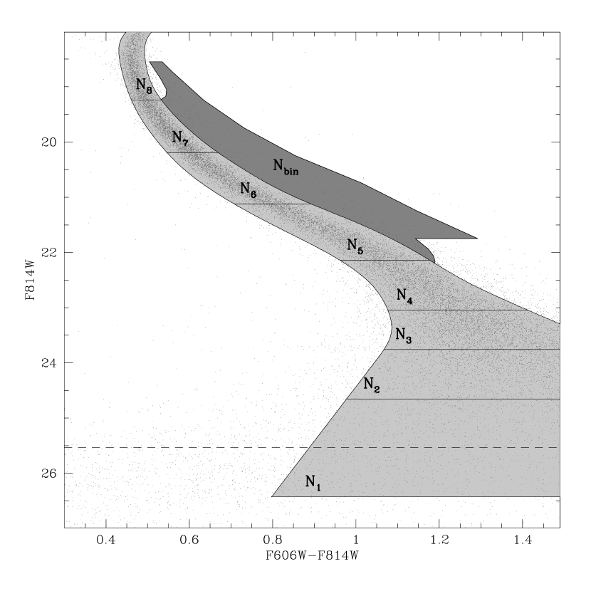
Figure 1.— Selection boxes adopted for the population of single stars (from $N_{1}$ to $N_{8}$) and binaries ($N_{bin}$) of NGC 288. The F814W-(F606W-F814W) color-magnitude diagram is overplotted. The magnitude corresponding to the 50% completeness is marked by dashed line.

Following the prescriptions of Gunn & Griffin (1979), the phase-space distribution of stars is given by the contribution of eight groups of masses with the distribution function

$$f(E,L) = \sum_{i=1}^{8}k_{i}exp\left(-\frac{A_{i}L^{2}}{2\sigma_{K}^{2}r_{a}^{2}}\right)\left[exp\left(-\frac{A_{i}E}{2\sigma_{K}^{2}}\right)-1\right]$$

$$\sum_{i=1}^{8}f_{i}(r,v_{r},v_{t}) = \sum_{i=1}^{8}k_{i}exp\left[-A_{i}\frac{v_{t}^{2}}{2\sigma_{K}^{2}}\left(\frac{r}{r_{a}}\right)^{2}\right]~{}\times$$

$$\left[exp\left(-\frac{A_{i}(v_{r}^{2}+v_{t}^{2}+2\psi)}{2\sigma_{K}^{2}}\right)-1\right]$$

where $E$ and $L$ are, respectively, the energy and angular momentum per unit mass, $v_{r}$ and $v_{t}$ are the radial and tangential components of the velocity, the effective potential $\psi$ is the difference between the cluster potential $\phi$ at a given radius r and the potential at the cluster tidal radius $\psi\equiv\phi-\phi_{t}$, $A_{i}$ and $k_{i}$ are scale factors for each mass group, and $\sigma_{K}$ is a normalization term. For each cluster we defined the eight mass bins (all covering equal mass intervals at different ranges) to sample the entire mass range from the hydrogen burning limit to the mass at the end of the Asymptotic Giant Branch evolution set by comparison between the CMD and the isochrones by Dotter et al. (2007)(see Fig. 1). The dependence on mass of the coefficients $A_{i}$ determines the degree of mass segregation of the cluster. Since the half-mass relaxation times of all the six GCs of our sample are significantly smaller than their ages (McLaughlin & van der Marel 2005) we adopted $A(i)\propto m_{i}$ (Michie 1963). The parameter $r_{a}$ determines the radius at which orbits become more radially biased. As $r_{a}\rightarrow\infty$, models become isotropic. As usual, the above distribution function has been integrated to obtain the number density and the radial and tangential components of the velocity dispersion of each mass group:

$$n_{i}(r) = 4\pi\int_{0}^{\sqrt{-2\psi}}\int_{0}^{\sqrt{-2\psi-v_{r}^{2}}}v_{t}f_{i}(r,v_{r},v_{t})dv_{t}dv_{r},$$

$$\sigma_{r,i}^{2} = \frac{4\pi}{\rho_{i}(r)}\int_{0}^{\sqrt{-2\psi}}v_{r}^{2}\int_{0}^{\sqrt{-2\psi-v_{r}^{2}}}v_{t}f_{i}(r,v_{r},v_{t})dv_{t}dv_{r},$$

$$\sigma_{t,i}^{2} = \frac{4\pi}{\rho_{i}(r)}\int_{0}^{\sqrt{-2\psi}}\int_{0}^{\sqrt{-2\psi-v_{r}^{2}}}v_{t}^{3}f_{i}(r,v_{r},v_{t})dv_{t}dv_{r}$$

The above equations can be written in terms of dimensionless quantities by substituting

$$\zeta = \frac{v_{r}^{2}}{2\sigma_{K}^{2}},\eta=\frac{v_{t}^{2}}{2\sigma_{K}^{2}},$$

$$\tilde{\rho}_{i} = \frac{m_{i}n_{i}}{\sum_{j}m_{j}n_{0,j}},\tilde{r}=\frac{r}{r_{c}},$$

$$W = -\frac{\psi}{\sigma_{K}^{2}},\tilde{r}_{a}=\frac{r_{a}}{r_{c}},$$

where $\rho_{0}$ is the central cluster density and

$$r_{c}\equiv\left(\frac{9\sigma_{K}^{2}}{4\pi G\rho_{0}}\right)^{1/2}$$

is the core radius (King 1966). The potential at each radius is determined by the Poisson equation

$$\nabla^{2}\psi=4\pi G\rho$$ (3)

Equations 3 and 3 have been integrated once assumed a value of the adimensional potential at the center $W_{0}$ outward till the radius $r_{t}$ at which both density and potential vanish. The total mass of the cluster $M$ is then given by the sum of the masses of all the groups

$$M = \sum_{i=1}^{8}m_{i}N_{i}$$

$$= \frac{9r_{c}\sigma_{K}^{2}}{G}\sum_{i=1}^{8}\int_{0}^{r_{t}}\tilde{\rho}_{i}\tilde{r}^{2}d\tilde{r}$$

As a last step, the above profiles have been projected on the plane of the sky to obtain the surface mass density

$$\Sigma_{i}(R)=2\int_{R}^{r_{t}}\frac{\rho_{i}r}{\sqrt{r^{2}-R^{2}}}dr$$

and the line-of-sight velocity dispersion

$$\sigma_{v,i}^{2}(R)=\frac{1}{\Sigma_{i}}\int_{R}{r_{t}}\frac{\rho_{i}[2\sigma_{r,i}^{2}(r^{2}-R^{2})+\sigma_{t,i}^{2}R^{2}]}{r\sqrt{r^{2}-R^{2}}}dr$$

In the above models the shape of the density and velocity dispersion profiles are completely determined by the parameters ($W_{0},\tilde{r}_{a},N_{i}$) while their normalization is set by the pair of parameters ($r_{c},M$).

For each choice of the above parameters a large number ($N_{tot}=10^{6}$) of particles has been randomly extracted from a continuous mass function which reproduces the number counts in each mass bin and distributed across the cluster according to their masses by interpolating through the density profiles of the various mass groups. For each particle the tangential and radial components of its velocity have been then extracted from the distribution function defined by eq. 3 and projected in an arbitrary direction . The masses of the particles have been converted in F814W and Johnson V magnitude adopting the mass-luminosity relation of Dotter et al. (2007). Isochrones has been selected adopting the metallicities by Carretta et al. (2009a) and their magnitudes have been converted from the absolute to the apparent plane adopting the distances and reddening by Paust et al. (2010), while ages have been chosen to match the turn-off morphology of each cluster. We adopted the reddening coefficients listed by Sirianni et al. (2005). The F606W magnitude has been instead assigned by interpolating on the MS mean ridge line of each cluster in the F814W-(F606W-F814W) CMD. The same procedure has been performed for a fraction $f_{b}$ of binaries and $f_{remn}$ of dark remnants whose masses and magnitudes have been assigned following the prescriptions described in Sect. 3.1. A synthetic Horizontal Branch (HB) has been simulated for each cluster using the tracks by Dotter et al. (2007), tuning the mean mass and mass dispersion along the HB to reproduce the observed HB morphology. Photometric errors and completeness corrections have been included in the following way: to each simulated particle we associated an artificial star within $10\arcsec$ and with input F814W magnitude within 0.25 mag. If the articial star is recovered its corresponding shifts in color and F814W magnitude have been then applied to the particle, while the particle has been removed if the associated artificial star has not been recovered in the output artificial star catalog. To account for Galactic field interlopers, we used the Galaxy model of Robin et al. (2003). A catalogue covering an area of 1 square degree around each cluster center has been retrieved. A subsample of stars has been randomly extracted from the entire catalogue scaled to the ACS field of view and the V and I Johnson-Cousin magnitudes were converted into the ACS photometric system by means of the transformations of Sirianni et al. (2005). The correction for photometric errors and incompleteness have been applied to this sample as for cluster stars. So, at the end of the above procedure according to a given choice of input parameters a mock cluster with masses, projected velocities and magnitudes accounting for observational effects has been produced.

3.1. Binaries and Dark Remnants

The presence of binaries can influence both the luminosity and the mass estimate of a cluster. Indeed, while the two components of the binary system contribute to the total budget of light and mass in the same way as if they were single stars, their mutual interaction has two important effects: i) since the two components are not resolved the binary system can share the same portion of the CMD with single stars of different mass (Malkov & Zinnecker 2001), and ii) from a dynamical point of view they behave as a single massive object so that, as energy equipartition is established, they present on average lower velocities and a more concentrated distribution with respect to single stars. The above characteristics make them more resistant to the process of mass-loss via evaporation and tidal shocks. It is therefore important to account for the presence of a fraction of unresolved binaries to properly model the PDMF of the cluster. To model the population of binaries we extracted $N_{bin}=2f_{b}N_{tot}$ stars from the Kroupa (2001) IMF in the mass range $0.1<M/M_{\odot}<7$ and paired them randomly. From the resulting sample we extracted a subsample of pairs according to a ”chance of pairing” calculated by imposing that i) the distribution of mass ratios f(q) (where $q=m_{2}/m_{1}$ is the ratio between the masses of the secondary and the primary components of each binary system) in the mass range $1<M/M_{\odot}<7$ results the same observed by Fisher et al. (2005) in their sample of spectroscopic binaries in the solar neighborhood, and ii) the distribution of systemic masses must be the same of single stars in the common mass range. The accepted pairs were added to a library of binaries while the rejected ones are ”broken” and their components have been used for the next iteration. The procedure has been repeated until all stars are included in the library. Then, all binaries whose primary component has a mass exceeding the maximum allowed for an evolving cluster star have been removed. The location and velocity of binaries within the cluster has been assigned according to their systemic mass (see Sect. 3). The relative projected velocity of the primary component has been added to the projected velocity of each binary according to the formula

$$v=\frac{2\pi a_{1}sini}{P(1-e^{2})^{1/2}}[cos(\theta+\omega)+ecos\omega]~{}~{}~{}~{}~{}~{}~{}~{}~{}\mbox{McConnachie \& C\^{o}te (2010)}$$

where $a_{1}$ is the semimajor axis of the primary component, $P$ is the orbital period, $e$ is the eccentricity, $i$ is the inclination angle to the line-of-sight, $\theta$ is the phase from the periastron, and $\omega$ is the longitude of the periastron. We followed the prescriptions of Duquennoy & Mayor (1991) for the distribution of periods and eccentricities. The semimajor axis has been calculated using Kepler’s third law:

$$a_{1}=\frac{1}{1+\frac{m_{1}}{m_{2}}}\left[\frac{P^{2}G(m_{1}+m_{2})}{4\pi^{2}}\right]^{1/3}$$

where $m_{1}$ and $m_{2}$ are the masses of the primary and secondary components.We removed all those binaries whose corresponding semimajor axes lie outside the range $a_{min}<a_{1}+a_{2}<a_{max}$ where $a_{min}$ is linked to the radius of the secondary component (according to Lee & Nelson 1988) and $a_{max}$ is set physically by the maximum separation beyond which the binary becomes unbound due to stellar interactions within the cluster (see eq. 1 of Hills 1984). The distribution of the angles (i, $\theta$, $\omega$) has been chosen according to the corresponding probability distributions (${\rm Prob}(i)\propto\sin i;{\rm Prob}(\theta)\propto\dot{\theta}^{-1};{\rm Prob}(\omega)={\rm constant}$). The magnitudes of the two components have been then estimated as for single stars and the overall magnitude has been calculated from the sum of their fluxes in the different passbands. The photometric errors and completeness correction have been then applied following the same procedure adopted for single stars (see Sect. 3).

The number of dark remnants (white dwarfs, neutron stars and black holes) has been estimated adopting for the precursors a Kroupa (2001) IMF normalized to the number of stars in the most massive stellar bin. We then adopted the initial-final mass relation and the retention fractions (for the initial velocity kicks) by Kruijssen (2009). We applied an additional correction to account for the selective removal of low-mass remnant as a result of tidal effects by imposing the same PDMF in the mass range in common with single stars.

4. method

Figure 2.— Comparison between three observables of NGC 288 (filled points) and the corresponding model prediction (solid lines). Upper-left panel: surface brightness profile; upper-right panel: velocity dispersion profile; bottom panels: F814W luminosity function in the inner (left) and outer (right) cluster regions.

The choice of the best model that reproduces the structure and kinematics of each cluster has been made by comparing simultaneously four observables measured on the databases and in the simulated mock cluster:

• The surface brightness profile;

• The F814W luminosity function;

• The fraction of binaries;

• The velocity dispersion profile.

The surface brightness profile of the mock cluster has been derived by summing the Johnson V fluxes of particles contained within circular concentric annuli of variable width and dividing the resulting flux by the annulus area. The widths of the annuli have been chosen to contain at least 20 stars to minimize Poisson noise while maintaining a good resolution in distance. A $\chi^{2}$ of the fit has been then calculated.

The comparison of the F814W luminosity function and of the binary fraction have been performed simultaneously by comparing the number counts ($N_{i}^{obs}$) in nine regions of the F814W-(F606W-F814W) CMD defined as follows: eight F814W magnitude intervals have been defined in correspondence to the mass bins adopted in the cluster modeling (see Sect. 3) and including all stars with colors within 3 times the photometric error corresponding to their magnitudes. A binary region has been defined within four boundaries: the selected stars are those contained in magnitude between the loci of binaries with primary star mass $m_{1}=0.45~{}M_{\odot}$ (faint boundary) and $m_{1}=0.75~{}M_{\odot}$ (bright boundary), and in color between the MS ridge line (blue boundary) and the equal-mass binary sequence (red boundary) both red-shifted by 3 times the photometric error (see Fig. 1; see also Sollima et al. 2007). We excluded the innermost $0.5\arcmin$ of the core-collapsed clusters NGC6752 and NGC7099 as in these extremely crowded regions the completeness level drops below 50% even at relatively bright magnitudes.

The velocity dispersion profile of the cluster has been compared using the likelihood merit function

$$l=\sum_{i=1}^{N}(-\frac{(v_{i}-\overline{v})^{2}}{\sigma_{v}(r_{i})^{2}+\delta v_{i}^{2}}-ln(\sigma_{v}^{2}+\delta v_{i}^{2}))$$ (4)

where $r_{i}$, $v_{i}$ and $\delta v_{i}$ are the distance to the cluster center, the radial velocity and the corresponding uncertainty of the i-th observed star, $\overline{v}$ is the mean velocity of the sample and $\sigma_{v}(r_{i})$ is the velocity dispersion predicted for RGB stars by the model at $r_{i}$. We excluded the outermost region of the cluster at $d>2~{}r_{h}$ to minimize the effect of tidal heating that can inflate the velocity dispersion in the outskirts of our clusters (Johnston et al. 1999; Kupper et al. 2010).

We adopted an iterative algorithm that starts from an initial guess of the parameters ($W_{0},r_{c},M,\tilde{r}_{a},N_{i},f_{b}$), generates the mock cluster and calculates the observables described above. Corrections to the parameters are then calculated using the method described below and the procedure is repeated until convergence. In each iteration the following steps are performed sequentially:

• 1. The value of $W_{0}$ and $r_{c}$ providing the best fit to the surface brightness profile are searched by minimizing the $\chi^{2}$ statistic. At the end of this step a new mock cluster is generated leaving the other parameters unchanged;

  2. The relative fraction of stars in the eight mass bins $N_{i}$ is adjusted by multiplying them for corrective terms which are proportional to the ratio between the number of objects in each bin of the observed and of the simulated CMDs.

     $$N_{i}^{\prime}=N_{i}\left(\frac{N_{i}^{obs}}{N_{i}^{mock}}\frac{\sum_{i=1}^{8}N_{i}^{mock}}{\sum_{i=1}^{8}N_{i}^{obs}}\right)^{\eta}$$

     where $N_{i}^{obs}$ and $N_{i}^{mock}$ are the number of stars counted in the i-th bin in the observed CMD and in simulated one, $N^{\prime}_{i}$ is the updated value of $N_{i}$ and $\eta$ is a softening parameter, set to 0.5, used to avoid divergence. An updated value for the binary fraction $f_{b}$ is also set using the same method. Then, a new mock cluster is generated and the procedure is repeated from point (1) until convergence.

• The above steps are repeated for different values of $\tilde{r}_{a}$ and the merit function $l$ is calculated by comparison with the radial velocities to determine the best-fit value of $\tilde{r}_{a}$.

The procedure usually converges after 10-20 iterations independently on the initial guess of parameters. Convergence is set when the various parameters start to fluctuate around the best-fit value with an amplitude (typically $<1\%$) linked to the degree of degeneracy among the various solutions. The uncertainty in the derived parameters has been calculated as the standard deviations of such fluctuations quadratically combined with the Poisson noise of star counts (only for the case of the $M$,$N_{i}$ and $f_{b}$ parameters). The mass of the model can be constrained in two independent ways: i) by best fitting the total number counts (so imposing $\sum_{i=1}^{8}N_{i}^{mock}=\sum_{i=1}^{8}N_{i}^{obs}$) or ii) by matching the amplitude of the velocity dispersion. The former estimate gives the stellar mass ($M_{*}$), the latter the dynamical one ($M_{dyn}$).

In Fig. 2 the comparison between the considered observables and the prediction of the best-fit model are shown for the case of NGC288. It is clear that the model well-reproduces the surface brightness and velocity dispersion profiles as well as the F814W luminosity functions measured in the two radial samples considered for this cluster. In this cluster, where ancillary observations are available in an external region, the model that best fit the inner sample observables also fits both the shape and the normalization of the luminosity function in the external sample. Although this agreement cannot guarantee the full adequacy of models and observables in the whole sample of clusters, it represents a sanity check supporting the validity of the assumptions made on mass segregation and on the star counts-surface brightness conversion.

5. Results

Table 1Best-fit parameters of the six target clusters

Name	$W_{0}$	$r_{c}$	$r_{c}$	$\tilde{r}_{a}$	$f_{b}$	$f_{b}^{core}$	$\alpha$	$log~{}M_{dyn}$	$log~{}M_{*}$	$M_{dyn}/L_{V}$	$M_{*}/L_{V}$
		$\arcmin$	pc		%	%		$M_{\odot}$	$M_{\odot}$	$M_{\odot}/L_{V,\odot}$	$M_{\odot}/L_{V,\odot}$
NGC 288	6.2	1.90	5.40	11	3.3$\pm$0.2	4.8$\pm 0.3$	-1.04$\pm$0.05	4.83$\pm$0.07	4.73$\pm$0.1	1.3$\pm$0.4	1.0$\pm$0.4
NGC 5024	11	0.55	2.99	+$\infty$	4.3$\pm$3.0	11.5$\pm$7.2	-1.08$\pm$0.07	5.60$\pm$0.07	5.61$\pm$0.1	1.5$\pm$0.3	1.5$\pm$0.4
NGC 6218	7.7	1.05	1.50	12	3.2$\pm$0.2	5.8$\pm$0.4	-0.22$\pm$0.02	4.90$\pm$0.05	4.74$\pm$0.1	1.0$\pm$0.3	0.7$\pm$0.2
NGC 6752	13	0.42	0.51	+$\infty$	0.6$\pm$0.1	3.6$\pm$0.6	-1.41$\pm$0.09	5.45$\pm$0.04	5.20$\pm$0.1	2.4$\pm$0.5	1.3$\pm$0.4
NGC 6809	5.5	2.50	3.32	4	2.5$\pm$0.2	3.4$\pm$0.3	-0.67$\pm$0.01	5.19$\pm$0.03	5.08$\pm$0.1	1.6$\pm$0.2	1.3$\pm$0.2
NGC 7099	13.5	0.13	0.34	+$\infty$	1.7$\pm$0.1	12.0$\pm$0.9	-1.14$\pm$0.04	5.28$\pm$0.05	5.08$\pm$0.1	2.1$\pm$0.4	1.3$\pm$0.3

The procedure described above allows to determine a set of parameters for the target clusters, in particular: their structural parameters, degree of anisotropy, binary fraction, PDMF and their stellar and dynamical masses. The best-fit parameters for each cluster are listed in Table 1. For completeness, the $M/L_{V}$ ratios, calculated from the V magnitudes by van den Bergh et al. (1991), are also listed. The structural parameter derived here are in good agreement with those estimated by previous studies (e.g. McLaughlin & van der Marel 2005). We note that all the clusters of our sample are best fitted by isotropic (or marginally anisotropic) models. However, the relatively large uncertainties in the binned velocity dispersion measures do not allow a meaningful analysis of this issue: the likelihood merit function $l$ (see Sect. 4) vary by less than 10% over a relatively large range of $\tilde{r}_{a}$ values in all cases.

The main results on the binary fraction, PDMF and mass are discussed in the following sections.

5.1. Binary fractions

Figure 3.— Derived fraction of binaries as a function of the dynamical mass.

The binary fractions listed in Table 1 are remarkably lower than those estimated in previous studies for the clusters in common (Sollima et al. 2007; Milone et al. 2012). This is related to the distribution of mass ratios adopted in this work that is different from those used in previous studies. The above difference can be well responsible for the observed discrepancies since in binaries with low mass ratios the contribution of the secondary component to the total flux is negligible, and they appear in the CMD almost indistinguishable from single stars. Therefore, the adoption of a mass ratio distribution skewed toward low (high) mass ratios produce a larger (smaller) correction for hidden binaries. To verify the consistency of our analysis with the previous works we calculated the fraction of binaries in NGC288 adopting a flat mass-ratios distribution over the entire mass range instead of the assumptions described in Sect. 3.1. In this case the overall binary fraction turns out to be $6.5\pm 0.3$% corresponding to $9.6\pm 0.4\%$ in the cluster core, in agreement within the errors with the estimates by Sollima et al. (2007) and Milone et al. (2012). It is worth noting that both the PDMF and the mass estimates are almost unaffected by this change: in this case in fact the slope of the PDMF varies of less than $\Delta~{}\alpha\simeq-0.07$ and both the dynamical and luminous masses remain the same within $\Delta logM/M_{\odot}<0.01$. So, although the adopted mass-ratio distribution is somehow arbitrary, it influences only the absolute fraction of binaries having a negligible effect on the relative cluster-to-cluster ranking, on the luminous and dynamical masses and on the shape of the PDMF.

In Fig. 3 the fraction of binaries of our sample of clusters are plotted as a function of the derived cluster dynamical mass. Once excluded NGC 5024 which has a large uncertainty in the derived binary fraction, a clear anticorrelation is noticeable with massive clusters hosting a smaller fraction of binaries. This result has been already observed in Milone et al. (2008, 2012) and Sollima et al. (2010) on a larger sample of clusters.

5.2. Present-Day Mass Function

Figure 4.— The present-day mass function of the six target clusters are shown. A vertical shift has been added for each cluster for clarity.

In Fig. 4 the global PDMFs of the six clusters are shown. The PDMFs can be well represented by single power laws whose slopes are all comprised within the range $-0.2<\alpha<-1.45$ being significantly less steep than the IMF of Salpeter (1955; $\alpha=-2.35$) and, in all but the case of NGC6752, of Kroupa (2001; $\alpha=-1.3$ at $M<0.5~{}M_{\odot}$ with a mean slope of $<\alpha>=-1.7$ between $0.3<M/M_{\odot}<0.8$). The exteme value for NGC 6218 ($\alpha=-0.22\pm 0.02$) confirms the peculiar flatness of the PDMF of this cluster already noticed by De Marchi et al. (2006). For the two clusters NGC 288 and NGC7099 in common with Paust et al. (2010) the derived slopes agree within the combined uncertainties of the two works ($\sim 0.2$). In the same way, the slopes derived for NGC 6809 and NGC 7099 agree to those estimated for these clusters by Piotto & Zoccali (1999) and Piotto et al. (1997), respectively. We find no signs of a turnover at low masses in all cases, although a convex shape of the PDMF is visible in NGC 5024. It is however worth noting that the mass at which the PDMF is expected to culminate is $\sim 0.3~{}M_{\odot}$ (Paresce & De Marchi 2000), so this last conclusion depends only on the relative fraction of stars in the lowest-mass bin. However, the estimate in this bin is by far the most uncertain since i) the mass-luminosity relation in this mass range is largely uncertain, ii) the completeness in this bin is low and uncertain, and iii) some contamination from faint unresolved galaxies falling in the large selection box of this mass bin (see Fig. 1) could be present. So, a firm conclusion on the presence of a turnover in the PDMF in these clusters cannot be established.

6. Dynamical versus stellar mass

Figure 5.— Left panel: comparison between the stellar and dynamical masses of the six target clusters. Right panel: comparison between the stellar masses measured in the present work and in McLaughlin & van der Marel (2005). The one-to-one relation is marked by the dashed line in both panels.

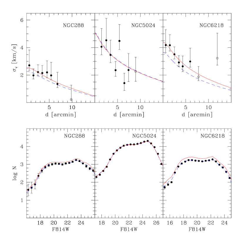
Figure 6.— Comparison of the observed velocity dispersion profile (top panels) and the F814W luminosity function (bottom panels) of the clusters NGC288 (left), NGC5024 (middle) and NGC6218 (right) with the corresponding models with the best-fit $M_{dyn}$ (solid lines; red in the online version) and $M_{*}$ (dashed lines; blue in the online version). The velocity dispersion measures not included in the analysis (at $d>2~{}r_{h}$) are marked with open points in upper panels.

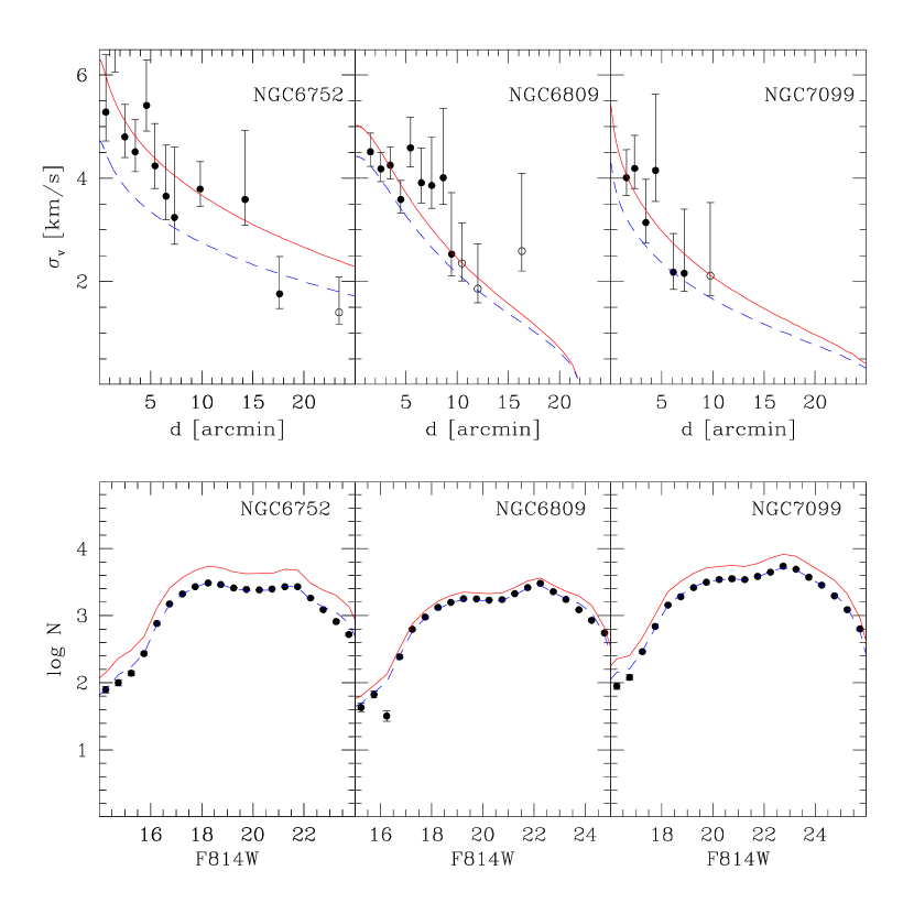
Figure 7.— Same of Fig. 6 for NGC6752 (left), NGC6809 (middle) and NGC7099 (right).

The main result of this analysis is the measure of the dynamical and stellar masses of the target clusters. Previous estimates of the dynamical mass of GCs have been made by Mandushev et al. (1991), Pryor & Meylan (1993), Lane et al. (2010a) and Zocchi et al. (2012) which have respectively 3, 5, 6 and 3 clusters in common with the present study. The mean differences and standard deviations between the dynamical masses estimated by these authors and those estimated here are $\Delta~{}log(M/M_{\odot})=$0.13($\sigma=$0.15), -0.03(0.17), 0.10(0.26) and -0.09(0.14), respectively, indicating a good agreement within the errors without significant systematics. In the right panel of Fig. 5 the derived stellar masses are compared with those reported by McLaughlin & van der Marel (2005) for the four clusters in common using the $M/L_{V}$ values predicted by the population synthesis model of Bruzual & Charlot (2003) adopting a Kroupa (2001) IMF. The stellar masses derived here are in reasonable agreement within the errors with those derived by these authors when considering individual clusters, although on average our estimates are smaller by $\sim$ 20%. This is expected since the Kroupa (2001) IMF is steeper than the PDMFs shown in Fig. 4 overestimating the number of low-mass stars that contribute significantly to the clusters’ mass budget and only marginally to their light.

From an inspection of Table 1 it is suddenly evident a discrepancy between the dynamical and stellar masses of five out of six clusters (with the exception of NGC 5024) with the dynamical masses systematically larger than the stellar ones by $\sim$40% . This is shown in the left panel of Fig. 5 where the two estimates are compared.

The observed difference between the dynamical and stellar masses can be also visualized in Fig. 6 and 7 where the velocity dispersion profile and of the F814W luminosity function of the six target clusters are compared with the prediction of the best-fit models with the appropriate $M_{*}$ and $M_{dyn}$. It is clear that, apart from the case of NGC5024, models are not able to fit simultaneously both the velocity dispersion profile and of the F814W luminosity function. Such a discrepancy is significant from a statistical point of view: a $\chi^{2}$ test indicates that the probability that the above difference occurs by chance in the entire sample of clusters is smaller than 3%. Such a discrepancy can be due to either observational biases in the determination of masses or to a physical reason. In the next sections we will analyze both possibilities.

6.1. Possible observational biases

To understand if the observed deficiency of stellar mass is real or due to an effect of the adopted technique we must search for some systematics in our analysis leading to an overestimate of the dynamical masses or to an underestimate of the stellar ones in all the six clusters of our sample.

The dynamical mass mainly follows from the fit of the velocity dispersion profile, therefore any systematics affecting the velocity dispersion can alter its determination. An obvious possibility is that the velocity errors reported by Lane et al. (2011) are underestimated. In fact, according to eq. 4, the observed velocity spread is given by the convolution of the ”true” velocity dispersion and the observational errors. So, for a given observed velocity spread, the larger are the errors the smaller is the estimated ”true” velocity dispersion and, consequently, the best-fit dynamical mass is expected to be smaller than estimated. However, the comparison with a high-resolution sample shown by Bellazzini et al. (2012) indicates a scatter compatible with (and even smaller than) the combined uncertainties of the two datasets. This is also in agreement with what is reported by Lane et al. (2011) who claim that the velocity uncertainties of their sample could be overestimated by $\sim$ 20%, making the difference even more striking.

The stellar mass depends mainly on the normalization between the observed and predicted F814W luminosity function and on the correction for the fraction of mass not covered by the ACS field of view. In all the analyzed clusters the samples of stars involved in the fit consist of more than 15000 stars, $\sim$90% of them are above the 80% level of completeness. So, the Poisson error due to number counts and to the error on the completeness correction are negligible ($\Delta logM_{*}/M_{\odot}<0.01$). A good correction for the radial coverage is supposed to be provided by the excellent fit of the surface brightness profile. However, we must stress that such profiles are constituted by a compilation of inhomogeneous data, often merging aperture photometric measurements (tracing the distribution of the brightest and most massive RGB stars) in the central part with star counts of (low-mass) MS stars in the outskirts. As stars with different masses have also different radial profiles (as a result of mass segregation), this introduces a large source of uncertainty in the fit. In this context, the simultaneous agreement between the predicted and observed F814W luminosity function of NGC 288 in both the internal and external fields is encouraging.

6.2. Effect of assumptions

Figure 8.— Projected density (left panel) and velocity dispersion (right panels) profiles calculated from the last snapshot of the N-body simulation. The quantities at the end of the simulation are marked with filled dots. The best-fit static model is overplotted in both panels with dashed lines.

If the discrepancy is not linked to any observational bias, it can be related to a physical effect not (properly) considered in our models. There are many possible mechanisms that may affect the mass determination. In this Section we evaluate the impact of the various input taking the cluster NGC288 as tester. In this cluster the observed mass discrepancy ($\Delta logM/M_{\odot}=0.1$) is smaller than the average of the six analysed GCs ($\Delta logM/M_{\odot}=0.18$) so that care should be taken in the general interpretation of the derived results.

As discussed in the previous section, the estimate of the dynamical mass is sensible to all the parameters affecting the velocity dispersion. Radial anisotropy can in principle distort the velocity dispersion profile, resulting in a different normalization of mass. As discussed in Sect. 5, we take into account for this effect in our models, but nevertheless the relatively large uncertainties in the velocity estimates do not allow a firm constraint on this quantity. To test this effect, we repeated the fit imposing the maximum degree of radial anisotropy that still ensures stability (see Nipoti et al. 2002). The largest effect on the derived dynamical mass has been found to be $\Delta~{}log~{}M_{dyn}/M_{\odot}\leq 0.03$. Binaries can also inflate the velocity dispersion because of the presence of the additional orbital motion of the binary components. Also in this case, while our code accounts for such an effect, a different assumption of the distribution of mass ratios might produce a difference. However, the test performed in Sect. 5.1 indicates that while the above assumption can affect significantly the fraction of binaries, the resulting mass is only marginally affected ($\Delta~{}log~{}M_{dyn}/M_{\odot}<0.01$). Another important effect is the heating due to the tidal interaction of the clusters with the Milky Way: the periodic shocks occurring every disk crossing and pericentric passage transfer kinetic energy to the cluster stars inflating its velocity dispersion, particularly in the outskirts (Gnedin & Ostriker 1997). While this effect is limited in our case since we excluded by the fit the outermost portion of the velocity dispersion profile, Kupper et al. (2010) showed that significant heating can occur also within the half-mass radius of lose clusters. To test this hypothesis, we run an N-body simulation to follow the structural and kinematical evolution of a cluster with the orbital and structural characteristics of NGC 288. This is the less dense cluster of our sample and should therefore be among those where tidal shocks are expected to produce the largest effect. We used the last version of the collisionless N-body code gyrfalcON (Dehnen 2000). The cluster has been represented by 61,440 particles distributed according to the best-fit multimass model of this cluster (see Table 1). The mean masses of the particles have been scaled to match the observed cluster mass. We adopted a leapfrog scheme with a time step of $\Delta t=1.45\times 10^{4}yr$ and a softening length of 0.43 pc (following the prescription of Dehnen & Read 2011). Such a relatively large time step and softening length do not affect the accuracy of the simulation because we are interested in the tidal effects which occur on a timescale significantly shorter than the relaxation time (the timescale at which collisions become important). The cluster was launched within the three-component (bulge + disk + halo) static Galactic potential of Johnston et al. (1995) with the energy and angular momentum listed by Dinescu et al. (1999) and its evolution has been followed for 0.852 Gyr (corresponding to 4 orbital periods). The projected density and velocity dispersion profiles at the end of the simulation are shown in Fig. 8. It is clear that the final velocity dispersion deviates from the prediction of the steady-state model at a distance of $\sim 4\arcmin\simeq r_{h}$ to the center. By applying the same technique described in Sect. 4 to the outcome of the simulation we overestimate the mass of the cluster by $\Delta~{}log~{}M_{dyn}/M_{\odot}\sim 0.06$.

The stellar mass can be underestimated because of an improper conversion between F814W magnitude and mass or because of the presence of non-luminous matter. Considering that the mass discrepancy is of the order of $\sim$40%, uncertainties on distance, reddening and age can be excluded as possible causes: to reproduce the above mass difference one should adopt for these clusters ages $<$4 Gyr, distance moduli shifted by $\sim$2.5 mag or reddening differences of $\Delta E(B-V)\sim$0.2, many orders of magnitudes larger than their statistical uncertainties. Uncertainties in the mass-luminosity relation can be also responsible for part of the discrepancy. In this regard, it is worth noting that while different stellar evolution models all agree for masses $M>0.1~{}M_{\odot}$ (Alexander et al. 1997; Baraffe et al. 1997; Dotter et al. 2007, Marigo et al. 2008) significant differences can be present in the least massive bin. Also in this case, however, the effect of such uncertainty is not expected to exceed few percent in the estimated mass. A larger effect is instead produced by the assumption on dark remnants. As described in Sect. 3.1, we followed the prescription by Kruijssen (2009) for the retention fraction of these objects and a Kroupa (2001) IMF for their precursors. To estimate the extent of the impact of this assumption we considered the extreme case of a 100% retention fraction for all the remnant. In this ideal case, the stellar mass would increase by $\Delta~{}log~{}M_{*}/M_{\odot}\sim 0.08$. The adoption of a different slope for the IMF has an even larger effect: the entire mass discrepancy could be completely removed by assuming a slope of $\alpha=-1.5$ (instead of -2.3) for masses $M>0.8M_{\odot}$, because the shallower the slope of the IMF is, the larger is the relative fraction of massive stars which terminated their evolution and are now in form of dark remnants.

7. Discussion

By comparing the most extensive photometric and spectroscopic surveys with suitable dynamical models we derived the global binary fraction, the PDMF of six Galactic GCs as well as their stellar and dynamical masses. The approach adopted here has the advantage to not require an a priori assumption of the $M/L$ ratio to estimate the stellar mass (as usually done in previous works; e.g. McLaughlin & van der Marel 2005) which is instead estimated via direct star counts in the CMD.

We confirm the anticorrelation between binary fraction and cluster mass already found in previous studies (Milone et al. 2008, 2012; Sollima et al. 2010) and explained as the consequence of the increased efficiency of the binary ionization process in massive clusters. Indeed, in massive clusters both the number of collisions and the mean kinetic energy of stellar encounters is larger resulting in a higher probability of ionization of multiple systems (Sollima 2008).

The PDMFs of the six clusters are well-represented by single power laws, although we cannot exclude a turnover at masses $M<0.2~{}M_{\odot}$, because of the uncertainty in the relative fraction of the least massive stars.

The stellar masses derived for these clusters are on average smaller than those predicted by population synthesis models. This is a consequence of the fact that the IMF adopted by these models is steeper that the actual PDMF of the considered clusters. This has been previously predicted by Kruijssen & Mieske (2009) as the result of the preferential loss of low-mass stars during the cluster evolution.

We found a discrepancy between the stellar and dynamical masses of five clusters. In particular, dynamical masses are on average $\sim$40% larger than stellar ones. Such a discrepancy is statistically significant when considering the entire sample of six clusters and could not be detected by previous studies because of the overestimate of the stellar mass mentioned above. Unfortunately, we cannot exclude that such a discrepancy is due to the presence of systematics affecting our estimates. In particular, a possible source of systematics is constituted by the inhomogeneity of the surface brightness profiles sample of Trager et al. (1995). However, if the detected difference would be real, a number of physical interpretations could be given. After a careful test on the effect of various assumptions and physical processes we found that a significant spurious increase of the estimated dynamical masses is given by the tidal heating which can reduce (but not eliminate) the observed discrepancy. On the other hand, the assumption on the distribution and retention of dark remnant has the largest impact on the estimated stellar masses. Part (up to 75%) of the observed mass difference can be indeed explained assuming that most the remnants, including the most massive neutron stars and black holes, are retained. This could be the case if the cluster mass at the moment of the SNe II explosion was large enough to trap the remnants, whose kinetic energy has been increased by the velocity kick following the explosion. The mass necessary to retain the majority of massive remnants is of $\sim 10^{7}~{}M_{\odot}$ (see Fig. 1 of Kruijssen 2009). Such a large mass is comparable with the initial mass predicted by D’Ercole et al. (2008) to ignite the self-enrichment process observed in most GCs (see Carretta et al. 2009b). Moreover, massive remants are expected to be more resistant to tidal stripping since tend to sink toward in the cluster core as a result of mass segregation. It is however worth noting that a retention fraction larger than 80% would require initial masses and an early mass loss history quite extreme, which has indeed been proposed in theoretical works to be the result of severe tidal shocking in the primordial environment of GCs (Elmegreen 2010; Kruijssen et al. 2012). An even larger effect is provided by the slope of the high-mass end of the IMF of the precursors which can drastically increase the amount of non-luminous mass. In this regard, a recent analysis by Marks et al. (2012) suggests that the slope of the IMF in the range $M>M_{\odot}$ could be actually shallower than the canonical Salpeter (1955) and Kroupa (2001) values with a dependence on density and metallicity. In this case, a slope $\alpha\simeq-1.5$ (instead of $\alpha=-2.3$ by Kroupa 2001) could account for the entire difference between the estimated stellar and dynamical masses. Such a variation would have strong implications on the evolution of the GC MF: in fact, while the largest mass contribution would be due to the increased number of white dwarfs, the consistent increase of the fraction of massive remnants (black holes and neutron stars) makes these objects the main drivers of the MF evolution. It is not clear if such IMF could actually evolve in the PDMF observed in these clusters.

Another possibility is that GCs contain a modest fraction of non-baryonic dark matter. In this case, it is possible that what we see now is the remnant of a larger halo lost during the interaction with the Milky Way (see Saitoh et al. 2006). Some amount of dark matter is also expected if some GCs are the remnants of past accretion events, as previously suggested by Freeman & Bland-Hawthorn (2002). However, given the involved uncertainties, all these hypotheses are merely speculative. Further studies will be needed to verify the above possibilities.

References

- Alexander et al. (1997) Alexander, D. R., Brocato, E., Cassisi, S., et al. 1997, A&A, 317, 90
- Anderson et al. (2008) Anderson, J., Sarajedini, A., Bedin, L. R., et al. 2008, AJ, 135, 2055
- Arellano Ferro et al. (2011) Arellano Ferro, A., Figuera Jaimes, R., Giridhar, S., et al. 2011, MNRAS, 416, 2265
- Baraffe et al. (1997) Baraffe, I., Chabrier, G., Allard, F., & Hauschildt, P. H. 1997, A&A, 327, 1054
- Baumgardt et al. (2009) Baumgardt, H., Côté, P., Hilker, M., et al. 2009, MNRAS, 396, 2051
- Bellazzini et al. (2012) Bellazzini, M., Bragaglia, A., Carretta, E., et al. 2012, A&A, 538, A18
- Bertin & Arnouts (1996) Bertin, E., & Arnouts, S. 1996, A&AS, 117, 393
- Bruzual & Charlot (2003) Bruzual, G., & Charlot, S. 2003, MNRAS, 344, 1000
- Carretta et al. (2009) Carretta, E., Bragaglia, A., Gratton, R., D’Orazi, V., & Lucatello, S. 2009a, A&A, 508, 695
- Carretta et al. (2009) Carretta, E., Bragaglia, A., Gratton, R., & Lucatello, S. 2009b, A&A, 505, 139
- D’Ercole et al. (2008) D’Ercole, A., Vesperini, E., D’Antona, F., McMillan, S. L. W., & Recchi, S. 2008, MNRAS, 391, 825
- De Marchi et al. (2010) De Marchi, G., Paresce, F., & Portegies Zwart, S. 2010, ApJ, 718, 105
- de Marchi et al. (2006) De Marchi, G., Pulone, L., & Paresce, F. 2006, A&A, 449, 161
- Dehnen (2000) Dehnen, W. 2000, ApJ, 536, L39
- Dehnen & Read (2011) Dehnen, W., & Read, J. I. 2011, European Physical Journal Plus, 126, 55
- Dinescu et al. (1999) Dinescu, D. I., Girard, T. M., & van Altena, W. F. 1999, AJ, 117, 1792
- Djorgovski & King (1984) Djorgovski, S., & King, I. R. 1984, ApJ, 277, L49
- Dotter et al. (2007) Dotter, A., Chaboyer, B., Jevremović, D., et al. 2007, AJ, 134, 376
- Duquennoy & Mayor (1991) Duquennoy, A., & Mayor, M. 1991, A&A, 248, 485
- Elmegreen (2010) Elmegreen, B. G. 2010, ApJ, 712, L184
- Fisher et al. (2005) Fisher, J., Schröder, K.-P., & Smith, R. C. 2005, MNRAS, 361, 495
- Freeman & Bland-Hawthorn (2002) Freeman, K., & Bland-Hawthorn, J. 2002, ARA&A, 40, 487
- Gnedin & Ostriker (1997) Gnedin, O. Y., & Ostriker, J. P. 1997, ApJ, 474, 223
- Gunn & Griffin (1979) Gunn, J. E., & Griffin, R. F. 1979, AJ, 84, 752
- Hack & Cox (2001) Hack, W., & Cox, C. 2001, Instrument Science Report ACS 2001-008, 10 pages, 8
- Harris (1996) Harris, W. E. 1996, AJ, 112, 1487
- Hills (1984) Hills, J. G. 1984, AJ, 89, 1811
- Johnston et al. (1999) Johnston, K. V., Sigurdsson, S., & Hernquist, L. 1999, MNRAS, 302, 771
- Johnston et al. (1995) Johnston, K. V., Spergel, D. N., & Hernquist, L. 1995, ApJ, 451, 598
- King (1966) King, I. R. 1966, AJ, 71, 64
- Krist et al. (2010) Krist, J., Hook, R., & Stoehr, F. 2010, Astrophysics Source Code Library, record ascl:1010.057, 10057
- Kroupa (2001) Kroupa, P. 2001, MNRAS, 322, 231
- Kruijssen (2009) Kruijssen, J. M. D. 2009, A&A, 507, 1409
- Kruijssen & Mieske (2009) Kruijssen, J. M. D., & Mieske, S. 2009, A&A, 500, 785
- Kruijssen et al. (2012) Kruijssen, J. M. D., Pelupessy, F. I., Lamers, H. J. G. L. M., et al. 2012, MNRAS, 421, 1927
- Küpper et al. (2010) Küpper, A. H. W., Kroupa, P., Baumgardt, H., & Heggie, D. C. 2010, MNRAS, 407, 2241
- Lane et al. (2009) Lane, R. R., Kiss, L. L., Lewis, G. F., et al. 2009, MNRAS, 400, 917
- Lane et al. (2010) Lane, R. R., Kiss, L. L., Lewis, G. F., et al. 2010b, MNRAS, 401, 2521
- Lane et al. (2010) Lane, R. R., Kiss, L. L., Lewis, G. F., et al. 2010a, MNRAS, 406, 2732
- Lane et al. (2011) Lane, R. R., Kiss, L. L., Lewis, G. F., et al. 2011, A&A, 530, A31
- Lee & Nelson (1988) Lee, H. M., & Nelson, L. A. 1988, ApJ, 334, 688
- Malkov & Zinnecker (2001) Malkov, O., & Zinnecker, H. 2001, MNRAS, 321, 149
- Mandushev et al. (1991) Mandushev, G., Staneva, A., & Spasova, N. 1991, A&A, 252, 94
- Marigo et al. (2008) Marigo, P., Girardi, L., Bressan, A., et al. 2008, A&A, 482, 883
- Marks et al. (2012) Marks, M., Kroupa, P., Dabringhausen, J., & Pawlowski, M. S. 2012, MNRAS, 422, 2246
- McConnachie & Côté (2010) McConnachie, A. W., & Côté, P. 2010, ApJ, 722, L209
- McLaughlin & van der Marel (2005) McLaughlin, D. E., & van der Marel, R. P. 2005, ApJS, 161, 304
- Michie (1963) Michie, R. W. 1963, MNRAS, 125, 127
- Mieske et al. (2008) Mieske, S., Hilker, M., Jordán, A., et al. 2008, A&A, 487, 921
- Milone et al. (2008) Milone, A. P., Piotto, G., Bedin, L. R., & Sarajedini, A. 2008, Mem. Soc. Astron. Italiana, 79, 623
- Milone et al. (2012) Milone, A. P., Piotto, G., Bedin, L. R., et al. 2012, A&A, 540, A16
- Nipoti et al. (2002) Nipoti, C., Londrillo, P., & Ciotti, L. 2002, MNRAS, 332, 901
- Paresce & De Marchi (2000) Paresce, F., & De Marchi, G. 2000, ApJ, 534, 870
- Paust et al. (2010) Paust, N. E. Q., Reid, I. N., Piotto, G., et al. 2010, AJ, 139, 476
- Piotto & Zoccali (1999) Piotto, G., & Zoccali, M. 1999, A&A, 345, 485
- Piotto et al. (1997) Piotto, G., Cool, A. M., & King, I. R. 1997, AJ, 113, 1345
- Pryor & Meylan (1993) Pryor, C., & Meylan, G. 1993, Structure and Dynamics of Globular Clusters, 50, 357
- Robin et al. (2003) Robin, A. C., Reylé, C., Derrière, S., & Picaud, S. 2003, A&A, 409, 523
- Saitoh et al. (2006) Saitoh, T. R., Koda, J., Okamoto, T., Wada, K., & Habe, A. 2006, ApJ, 640, 22
- Salpeter (1955) Salpeter, E. E. 1955, ApJ, 121, 161
- Sarajedini et al. (2007) Sarajedini, A., Bedin, L. R., Chaboyer, B., et al. 2007, AJ, 133, 1658
- Simon et al. (2011) Simon, J. D., Geha, M., Minor, Q. E., et al. 2011, ApJ, 733, 46
- Sirianni et al. (2005) Sirianni, M., Jee, M. J., Benítez, N., et al. 2005, PASP, 117, 1049
- Sollima (2008) Sollima, A. 2008, MNRAS, 388, 307
- Sollima et al. (2010) Sollima, A., Carballo-Bello, J. A., Beccari, G., et al. 2010, MNRAS, 401, 577
- Sollima et al. (2007) Sollima, A., Beccari, G., Ferraro, F. R., Fusi Pecci, F., & Sarajedini, A. 2007, MNRAS, 380, 781
- Strader et al. (2011) Strader, J., Caldwell, N., & Seth, A. C. 2011, AJ, 142, 8
- Strader et al. (2009) Strader, J., Smith, G. H., Larsen, S., Brodie, J. P., & Huchra, J. P. 2009, AJ, 138, 547
- Tollerud et al. (2011) Tollerud, E. J., Bullock, J. S., Graves, G. J., & Wolf, J. 2011, ApJ, 726, 108
- Trager et al. (1995) Trager, S. C., King, I. R., & Djorgovski, S. 1995, AJ, 109, 218
- van den Bergh et al. (1991) van den Bergh, S., Morbey, C., & Pazder, J. 1991, ApJ, 375, 594
- Wilson (1975) Wilson, C. P. 1975, AJ, 80, 175
- Zocchi et al. (2012) Zocchi, A., Bertin, G., & Varri, A. L. 2012, A&A, 539, A65