Tau-Function Theory of Chaotic Quantum Transport with $\beta=1,2,4$

Abstract.

We study the cumulants and their generating functions of the probability distributions of the conductance, shot noise and Wigner delay time in ballistic quantum dots. Our approach is based on the integrable theory of certain matrix integrals and applies to all the symmetry classes $\beta\in\left\{1,2,4\right\}$ of Random Matrix Theory. We compute the weak localization corrections to the mixed cumulants of the conductance and shot noise for $\beta=1,4$, thus proving a number of conjectures of Khoruzhenko et al. [51]. We derive differential equations that characterize the cumulant generating functions for all $\beta\in\left\{1,2,4\right\}$. Furthermore, when $\beta=2$ we show that the cumulant generating function of the Wigner delay time can be expressed in terms of the Painlevé III^′ transcendant. This allows us to study properties of the cumulants of the Wigner delay time in the asymptotic limit $n\to\infty$. Finally, for all the symmetry classes and for any number of open channels, we derive a set of recurrence relations that are very efficient for computing cumulants at all orders.

1. Introduction

1.1. Background

Many successful approaches to tackle problems in quantum transport are based on the the Landauer-Büttiker scattering theory of electronic conduction (see, for example, the review article [14] and references therein). It applies to two very general types of systems: the first are mesoscopic conductors confined in space, often referred to as quantum dots, through which the electric current flows via two point contacts; the second are quasi-one dimensional wires containing scattering impurities. The physical dimensions of these systems are small enough that the quantum mechanical phase coherence of the electron is important and its properties cannot be understood in terms of classical mechanics; at the same time they are large enough that a statistical description of the electrical current becomes meaningful.

In 1985 Altshuler [11] and independently Lee and Stone [58] discovered that the statistical fluctuations of the conductance in disordered wires are universal. More precisely, they are independent of the dimensions of the sample or the strength of the disorder provided that the aspect ratio $\mathrm{length/width}\gg 1$, the length is much longer than the electron mean free path and much shorter than the localization length. Soon afterwards this phenomenon was observed experimentally [89]. Approximately at the same time, in a different area of physics, it was discovered that as $\hbar\to 0$ the correlations of the spectra of quantum systems with a chaotic classical limit are the same as those of the eigenvalues of random matrices from appropriate ensembles [22, 19]. It was then realised that Random Matrix Theory (RMT) could provide the mathematical framework to develop a statistical theory of quantum transport that would account for the universality of the fluctuations of the electric current [46, 45, 12, 13, 47].

The main hypothesis behind the RMT approach to quantum transport is that the average dwell time of the scattering electron is much larger than the Ehrenfest time, so that the system-specific features of the conductor become negligible and physical quantities can computed through appropriate ensemble averages, which depend only on the symmetries of the system. In this paper we focus on quantum dots connected to the environment via ideal leads, or, equivalently, through ballistic point contacts. Under these assumptions, the scattering matrix is uniformly distributed in one of Dyson’s circular ensembles [20, 21, 13, 12, 47]: the COE ($\beta=1$), CUE ($\beta=2$) and CSE ($\beta=4$), depending on whether the system has time-reversal and/or spin-rotational symmetry. In superconducting (Andreev) quantum dots additional constraints imply that the relevant symmetry classes are those discovered by Zirnbauer [91] and Altland and Zirnbauer [9, 10].

The subjects of this paper are the cumulants and their generating functions of the probability distributions of the electrical conductance, the shot noise, which is the time average of the current fluctuations at zero temperature, and the Wigner delay time, which is a measure of the extra time an electron spends in the scattering region. The Landauer formula expresses the conductance as a sum of the transmission eigenvalues, $T_{1},\dotsc,T_{n}$, where $n$ is the number of travelling modes (quantum channels) available to the electron wavefunction incoming, or outgoing, at one of the two edges of the conductor. It follows that both conductance and shot noise are linear statistics of $T_{1},\dotsc,T_{n}$. More precisely, they are

(1.1) $$G/G_{0}:=\sum_{j=1}^{n}T_{j}\quad\text{and}\quad P/P_{0}:=\sum_{j=1}^{n}T_{j}(1-T_{j}),$$

respectively. The constant $G_{0}:=2e^{2}/h$ is the unit of quantum conductance and $P_{0}:=2eVG_{0}$. Here $V$ is the voltage difference between the two edges of the conductor. In what follows we shall always choose units where $G_{0}=P_{0}=1$. The Wigner delay time is the average of the proper delay times, $\tau_{1},\dotsc,\tau_{n}$, namely

(1.2) $$\tau_{\mathrm{W}}:=\frac{1}{n}\sum_{j=1}^{n}\tau_{j},$$

where in this case $n$ is the total number of quantum channels. As we shall discuss in detail in Sec. 1.2, RMT predicts that the random variables $T_{j}$ are distributed like the spectra of matrices in the Jacobi Ensembles [12, 14, 37, 30], while the proper delay times like the inverse of the eigenvalues of matrices in the Laguerre Ensembles [26]. In the limit $n\to\infty$ the conductance, shot noise and Wigner delay time converge to normal random variables (see, e.g., [74, 87, 88]).

In this article we compute the first corrections to the semiclassical limit $n\to\infty$, often referred to as weak localisation corrections, of the mixed cumulants of $G$ and $P$ for $\beta=1,4$. We also calculate the leading order contributions to the cumulants of the Wigner delay time. In addition, we derive a set of differential equations that are satisfied by the cumulant generating functions for all $\beta\in\left\{1,2,4\right\}$. In particular, we prove that when $\beta=2$ the cumulant generating function of $\tau_{\mathrm{W}}$ can be expressed in terms of a solution of the Painlevé III^′ equation.

For over twenty years the universal properties of both linear and non-linear statistics of the transmission eigenvalues and the proper delay times have been extensively studied using both RMT [59, 40, 39, 76, 51, 69, 70, 72, 80, 73, 56, 57, 77, 78, 81, 79, 61, 64, 65, 87, 88] and periodic orbit theory [85, 75, 84, 60, 67, 68, 25, 43, 54, 55, 15, 16, 17, 18, 53]. Nevertheless, the higher moments and cumulants of $G$, $P$ and $\tau_{\mathrm{W}}$ appeared to be elusive for a long time and considerable effort was spent to investigate the lower cumulants [40, 76, 78, 79, 80, 77, 81]. This is hardly surprising, as the global fluctuations of the spectra of random matrices are particularly difficult to probe and few results are available [49, 34, 52, 24, 23, 35]. In the case of the Wigner delay time, the problem is further complicated by the fact that the right-hand side of Eq. (1.2) is a singular linear statistic on the eigenvalues of matrices in the Laguerre Ensembles. Furthermore, the appropriate Laguerre Ensemble contains an unusual $n$-dependent exponent (see Eq. (1.11)). As is often the case in RMT, ensembles with symmetries $\beta=1$ and $\beta=4$ are more difficult to deal with than those with $\beta=2$.

Recently Osipov and Kanzieper [72, 73] made substantial progress by using the theory of integrable systems combined with RMT to study the cumulant generating functions of the conductance and shot noise. They proved that when time-reversal symmetry is broken, the cumulant generating function of the conductance can be expressed in terms of a solution to the Painlevé V equation. They also computed the leading order terms of the cumulants in the limit as $n\to\infty$. Independently, Novaes [70] using Selberg’s integral discovered a finite $n$ formula for the moments of the conductance for $\beta=2$ as a sum over partitions. Soon afterward Khoruzhenko et al [51] made a further considerable contribution by combining generalizations of Selberg’s integral with the theory of symmetric functions. In particular, these techniques allowed them to compute the first asymptotic correction of the cumulants of conductance and shot noise when $\beta=2$. They were able to formulate conjectures for the same quantities for ensembles with $\beta=1$ symmetries, which until then had been much more difficult to tackle than the case $\beta=2$. In a recent letter Vidal and Kanzieper [86] computed the joint probability density function of the reflection eigenvalues in quantum dots with broken time reversal and coupled to the environment via point contacts with tunnel barriers.

Our approach is based on the integrable theory of certain classes of matrix integrals first introduced in [66, 42, 83] and then developed to its full potential by Adler, Shiota and van Moerbeke [2, 3, 4] and by Adler and van Moerbeke [5, 6, 7, 8]. Using this formalism, we show that the mixed cumulant generating function of the conductance and shot noise satisfies a certain non-linear PDE, which can be reduced to a set of recurrence relations for the cumulants of the conductance and the joint cumulants of conductance and shot noise. By looking at the leading order contribution to such difference equations, we can prove the conjectures of Khoruzhenko et al. [51] on the cumulants of conductance and shot noise when $\beta=1$, as well as perform the same analysis when $\beta=4$.

These techniques are powerful enough to cope with singularities of the linear statistics (1.2) too. Indeed, we can apply the same approach to the distribution of $\tau_{\mathrm{W}}$ and prove a number of finite $n$ properties that were previously beyond reach. These include recurrence relations for the cumulants for all $\beta\in\{1,2,4\}$, as well as the link between the Painlevé $\mathrm{III}^{\prime}$ equation and the cumulant generating function when $\beta=2$.

1.2. The Landauer-Büttiker Theory and Random Matrix Theory

The dynamics of an electron in a mesoscopic conductor can be studied by looking at its scattering by a two-dimensional ballistic cavity whose classical dynamics is chaotic. The scattering region is connected to two electron reservoirs in equilibrium at zero temperature and Fermi energy $E_{\mathrm{F}}$ by two ideal leads, which support a finite number of propagating modes (quantum channels). At low voltage the electron-electron interactions are negligible and the scattering is elastic. Therefore, the scattering matrix at energy $E$ relative to $E_{\mathrm{F}}$ is unitary and has the block structure

(1.3) $$S(E):=\begin{pmatrix}r_{m\times m}&t_{m\times n}^{\prime}\\ t_{n\times m}&r_{n\times n}^{\prime}\end{pmatrix}.$$

Here $m$ and $n$ are the numbers of channels in the left and right leads, respectively; the sub-blocks $r_{m\times m}$, $t_{n\times m}$ are the reflection and transmission matrices through the left lead and $r^{\prime}_{n\times n}$ and $t^{\prime}_{m\times n}$ those through the right lead. Without loss of generality we shall assume that $m\geq n$. The unitary matrix in (1.3) is often referred to as the Landauer-Büttiker scattering matrix. In this setting the semiclassical limit $\hbar\to 0$ is equivalent to $n\to\infty$ while the ratio $m/n$ remains finite.

The transmission eigenvalues $T_{1},\dotsc,T_{n}$ are the eigenvalues of the Hermitian matrix $tt^{\dagger}$ as well as of $t^{\prime\dagger}t^{\prime}$; thus, formulae (1.1) become

(1.4) $$G=\operatorname{Tr}tt^{\dagger}\quad\text{and}\quad P=\operatorname{Tr}\bigl{(}tt^{\dagger}(I-tt^{\dagger})\bigr{)}.$$

Since $S(E)$ is unitary, $T_{j}\in[0,1]$ for $j=1,\dotsc,n$. The proper delay times are the eigenvalues of the Wigner-Smith time-delay matrix, which is defined by

(1.5) $$Q:=-i\hbar S^{-1}(E)\frac{\partial S(E)}{\partial E}.$$

Thus, the Wigner delay time is the normalized trace

(1.6) $$\tau_{\mathrm{W}}=\frac{1}{n}\operatorname{Tr}Q.$$

Note that when we discuss the conductance and shot noise, $n$ denotes the number of quantum channels in one lead and not the dimensions of the scattering matrix, which are $(m+n)\times(m+n)$. When we consider the Wigner delay time, $n$ is the total number of channels; thus, in this case the dimensions of $S(E)$ and of $Q$ are $n\times n$. We adopt this convention to simplify the notation in the rest of the paper, since $n$ will always be the asymptotic parameter.

Within the RMT approach to quantum transport, the transmission matrix $tt^{\dagger}$ belongs to one of the Jacobi Ensembles; therefore, the joint probability density function (j.p.d.f.) of $T_{1},\dotsc,T_{n}$ is [12, 14, 37, 30]

(1.7) $$P_{\mathrm{J}}(T_{1},\dotsc,T_{n})=\frac{1}{c^{(\beta)}_{n}}\prod_{j=1}^{n}T_{j}^{\alpha}\left(1-T_{j}\right)^{\delta/2}\prod_{1\leq j<k\leq n}\left.\lvert T_{k}-T_{j}\right\rvert^{\beta},$$

where $\alpha=\frac{\beta}{2}\left(m-n+1\right)-1$ and

(1.8) $$\begin{split}c_{n}^{(\beta)}&:=\int_{[0,1]^{n}}\prod_{j=1}^{n}T_{j}^{\alpha}\left(1-T_{j}\right)^{\delta/2}\prod_{1\leq j<k\leq n}\left.\lvert T_{k}-T_{j}\right\rvert^{\beta}dT_{1}\dotsm dT_{n}\\ &=\prod_{j=0}^{n-1}\frac{\Gamma\left(\alpha+1+j\beta/2\right)\Gamma\left(\delta/2+1+j\beta/2\right)\Gamma\bigl{(}1+(j+1)\beta/2\bigr{)}}{\Gamma\bigl{(}\alpha+\delta/2+2+\left(n+j-1\right)\beta/2\bigr{)}\Gamma\left(1+\beta/2\right)}\end{split}$$

is Selberg’s integral (see, e.g., [38], Ch. 4). If the scattering matrix $S(E)$ belongs to one of Dyson’s ensembles then $\delta=0$. When additional constraints are imposed new symmetry classes may arise. In mesoscopic physics this happens when a chaotic cavity is in contact with a superconductor (Andreev quantum dots). The symmetry classes for these systems were predicted by Zirnbauer [91] and Altland and Zirnbauer [9, 10]. Dueñez [33] studied these symmetry classes too, and extended Zirnbauer’s theory. The new ensembles modelling the scattering matrix of Andreev quantum dots are the compact symmetric spaces that, according to Cartan’s classification, are of symmetry types C, CI, D and DIII. Such symmetries affect the dependence on the integers $(\beta,\delta)$ of the j.p.d.f. (1.7). More precisely, the connection between the symmetry class of $S(E)$ and $(\beta,\delta)$ is the following [30]:

$$(\beta,\delta) =(4,2), (\beta,\delta) =(2,1),$$ symmetry type C; symmetry type CI;

$$(\beta,\delta) =(1,-1), (\beta,\delta) =(2,-1),$$ symmetry type D; symmetry type DIII.

Physically, they correspond to different combinations of spin-rotation and time-reversal symmetries.

If the $T_{1},\dotsc,T_{n}$ were independent random variables, then the central limit theorem asserts that the variances of $G$ and $P$ would grow in proportion to $n$; instead, it remains finite in the limit $n\to\infty$. More specifically, we have [46, 13, 12, 47]

(1.9) $$\lim_{n\to\infty}\operatorname{Var}(G)=\frac{1}{8\beta}\quad\text{and}\quad\lim_{n\to\infty}\operatorname{Var}(P)=\frac{1}{64\beta}.$$

This phenomenon is a manifestation of the universal conductance fluctuations and is due to the strong correlations among the transmission eigenvalues, caused by the factor $\prod_{1\leq j<k\leq n}\left\lvert T_{k}-T_{j}\right\rvert^{\beta}$ in the right-hand side of (1.7). It is a common property for the spectra of random matrices. Similar central limit theorems on linear statistics of eigenvalues have been proved for the classical compact groups [32, 31, 48], the Gaussian, Jacobi and Laguerre Ensembles [49, 34, 35].

Braun et al. [25] and Heusler et al. [43] developed a semiclassical derivation of the average and variance of $G$ as well as of the average of $P$, which at the time was still unknown, to all orders in $1/n$. Shortly after, Savin and Sommers [78] reproduced the semiclassical results using Selberg’s integral. Subsequently, the same techniques allowed Sommers et al. [81] and Savin et al. [79] to compute the variance of $P$ and the first four cumulants of $G$ non-perturbatively.

The probability distributions of $P$ and $G$ are strongly non-Gaussian for small numbers of quantum channels [81, 51, 56]. In the large-$n$ limit they approach a universal Gaussian curve and contain weak singularities which have been investigated using large deviation estimates by Vivo et al. [87, 88]. Furthermore, Khoruzhenko et al. [51] derived exact Fourier series representations of these distributions; however, the coefficients of such series involve $n\times n$ determinants ($\beta=2$) or Pfaffians ($\beta=1$ or $\beta=4$) which are difficult to handle explicitly.

When the scattering matrix belongs to one of Dyson’s circular ensembles, then the j.p.d.f. of the proper delay times is [26]

(1.10) $$P_{\mathrm{W}}(\tau_{1},\ldots,\tau_{n})=\frac{1}{Z}\prod_{j=1}^{n}\tau_{j}^{-b}e^{-\frac{\beta\tau_{\mathrm{H}}}{2\tau_{j}}}\prod_{1\leq j<k\leq n}\left\lvert\tau_{k}-\tau_{j}\right\rvert^{\beta},$$

where $Z$ is a normalization constant, $\tau_{\mathrm{H}}$ is the Heisenberg time and

(1.11) $$b=\frac{3\beta n}{2}+2-\beta.$$

In our choice of units $\tau_{\mathrm{H}}=n$. The substitution $x_{j}=1/\tau_{j}$, $j=1,\dotsc,n$, turns (1.10) into the j.p.d.f. of the eigenvalues of matrices in the Laguerre Ensembles.

The singularities in the right-hand side of Eq. (1.10) make the Wigner delay time considerably more challenging to study than the conductance and shot noise; indeed, much less is known about the probability distribution of $\tau_{\mathrm{W}}$. Lehmann et al. [59] studied the parametric correlations of $\tau_{\mathrm{W}}$ when $\beta=1$ for small and large number of quantum channels using supersymmetry techniques in RMT. Fyodorov and Sommers [40] computed the finite $n$ parametric correlations as well as the variance when $\beta=2$. Furthermore, Fyodorov et al. [39] derived the crossover of the same quantities to systems with $\beta=1$. Kuipers and Sieber [55] computed such correlations as well as the first seven terms in the asymptotic expansion of the variance using periodic orbit theory for $\beta=1$ and $\beta=2$ symmetries. Semiclassical calculations to all orders in $1/n$ are still an open problem in this case. The distribution of the Wigner delay time for small numbers of channels as well as its transition to non-ideal coupling was treated in [76, 80, 77] for each of the Wigner-Dyson symmetry classes. Recently, Texier and Majumdar [82] studied the large deviations in the tails of the distribution of $\tau_{\mathrm{W}}$.

2. Main Results and Discussions

2.1. Conductance and Shot Noise

The definitions (1.1) and the j.p.d.f. (1.7) imply that the random variables $G$ and $P$ are correlated. The joint moment generating function

(2.1) $$\begin{split}\mathcal{M}^{(\beta)}_{n}(z,w)&:=\frac{1}{c^{(\beta)}_{n}}\int_{[0,1]^{n}}\prod_{j=1}^{n}T_{j}^{\alpha}(1-T_{j})^{\delta/2}\\ &\quad\times\exp\bigl{(}-zT_{j}-wT_{j}(1-T_{j})\bigr{)}\prod_{1\leq j<k\leq n}\left\lvert T_{k}-T_{j}\right\rvert^{\beta}dT_{1}\dotsb dT_{n}\end{split}$$

contains all the information on the joint probability density function of $G$ and $P$. By definition the joint cumulants $\kappa^{(\beta)}_{l,k}$ are the coefficients in the Taylor expansion

(2.2) $$\sigma^{(\beta)}_{n}(z,w):=\log\mathcal{M}^{(\beta)}_{n}(z,w)=\sum_{l=0}^{\infty}\sum_{k=0}^{\infty}\frac{(-1)^{l+k}\kappa^{(\beta)}_{l,k}}{l!k!}z^{l}w^{k}.$$

Since $\mathcal{M}_{n}^{(\beta)}(0,0)=1$, $\kappa^{(\beta)}_{0,0}=0$. The cumulants of the conductance or of the shot noise are obtained as special cases by setting $w=0$ or $z=0$ separately in (2.2); throughout this paper we will reserve the notation $\kappa^{(\beta)}_{l}:=\kappa^{(\beta)}_{l,0}$ for the cumulants of the conductance.

As $n,m\to\infty$ and $m-n$ remains finite, the averages of the conductance and shot noise are given by,

(2.3) $$\kappa_{1}^{(\beta)}=\frac{n}{2}+O(1)\quad\text{and}\quad\kappa_{0,1}^{(\beta)}=\frac{n}{8}+O(1);$$

the limit of the variances as $n\to\infty$ are given in Eq. (1.9).

One of the main problems addressed in this work concerns the asymptotics of the higher cumulants.

Theorem 2.1.

Let $\beta=1,4$ and suppose that $\alpha$ is independent of $n$, i.e. $m=n+C$ for some constant $C$. Then, we have

(2.4a) $$\lim_{n\to\infty}n^{l+k}\kappa^{(\beta)}_{l,k} =\bigl{(}\delta/2-\alpha\bigr{)}\bigl{(}\alpha+\delta/2+2-\beta\bigr{)}\frac{(k+l-1)!}{\beta(2\beta)^{l}(4\beta)^{k}},$$

for $$l (l,k)\neq(1,0)$$ odd and ,

(2.4b) $$\lim_{n\to\infty}n^{l+k-1}\kappa^{(\beta)}_{l,k} =(-1)^{k}\left(\frac{\beta}{2}-1\right)\frac{(l+k-2)!}{(4\beta)^{k}(4\beta)^{l}}\sum_{j=0}^{k}\binom{2j+l}{j+l/2}\binom{k}{j}(-2)^{-j},$$

for $$l (l,k)\notin\{(0,0),(0,1),(0,2),(2,0)\}$$ even and .

There are some interesting consequences of this theorem that are worth emphasizing.

Remark 2.2.

Let $\beta=1$ and $\delta=0$. In other words, consider normal (non-superconducting) quantum dots with time-reversal and spin-rotation symmetries. Assume also that the number of quantum channels is the same in both leads, i.e. $m=n$ and $\alpha=-1/2$, see Eq. (1.7). Khoruzhenko, Savin and Sommers [51] conjectured the weak localization corrections of the higher cumulants of the conductance:

(2.5a) $$\lim_{n\to\infty}n^{l}\kappa^{(1)}_{l} =\frac{(l-1)!}{2^{l+2}}, l$$ for odd,

(2.5b) $$\lim_{n\to\infty}n^{l-1}\kappa^{(1)}_{l} =-\frac{(l-2)!}{2^{2l+1}}\binom{l}{l/2}, l$$ for even

with $l>2$. Equations (2.5a) and (2.5b) are particular cases of Theorem 2.1.

In the same article it was also conjectured that at leading order the higher cumulants of the shot noise power are

(2.6a) $$\lim_{n\to\infty}n^{k}\kappa^{(1)}_{0,k} =\frac{(k-1)!}{2^{2k+3}}, k$$ for odd,

(2.6b) $$\lim_{n\to\infty}n^{k-1}\kappa^{(1)}_{0,k} =-\frac{(k-2)!}{2^{3k+1}}\binom{k}{k/2}, k$$ for even,

with $k>2$. When $l=0$ the sum in (2.4b) is given by

(2.7) $$\begin{split}\sum_{j=0}^{k}\binom{2j}{j}\binom{k}{j}(-2)^{-j}&=P_{k}^{(0,-k-\frac{1}{2})}(-3)=\frac{(-1)^{k/2}\sqrt{\pi}}{\Gamma\left(-\tfrac{k}{2}+\tfrac{1}{2}\right)\Gamma\left(\tfrac{k}{2}+1\right)}\\ &=\begin{cases}0,&\text{for $k$ odd,}\\ \frac{1}{2^{k}}\binom{k}{k/2},&\text{for $k$ even,}\end{cases}\end{split}$$

where $P_{k}^{(a,b)}(x)$ denotes the Jacobi polynomial (see Appendix C for the definition). The identity  (2.7) reduces formula (2.4b) to the right-hand side of (2.6b) when $k$ is even; however, mutual cancellations occur in the sum (2.7) when $k$ is odd, which yields

(2.8) $$\lim_{n\to\infty}n^{k-1}\kappa_{0,k}^{(1)}=0.$$

This limit implies that the first corrections to the odd cumulants of $P$ are of subleading order in $1/n$ and is consistent with the conjecture (2.6a). These cancellations explain the unusual “staircase” behaviour in the decay of the cumulants of the shot noise, first observed in [51].

As we shall discuss in Secs. 5.3, 5.4 and 5.5, the last step in proving Theorem 2.1 consists in solving the asymptotic limit of certain difference equations. As it turns out, proving formula (2.6a) requires computing the next to leading order of the mixed cumulants $\kappa^{(1)}_{l,k}$. Although in principle our techniques could be carried out at the next order in $1/n$, the calculations become substantially harder (see Sec. 5.5).

Remark 2.3.

Theorem 2.1 reveals some general qualitative differences among the probability distributions of $G$ and $P$ for the various symmetry classes.

In the special case $(\beta,\delta)=(2,0)$, i.e. when the Landauer-Büttiker scattering matrix belongs to the CUE, the cumulants of conductance and shot noise were computed to leading order by Osipov and Kanzieper [72, 73]. They are of subleading order in $1/n$ compared to formulae (2.4), which means that the convergence of $G$ and $P$ to a normal random variable is slower when $\beta=1$ and $\beta=4$. Similarly, the fact that the mixed cumulants are of lower order for $\beta=2$ [73] implies that the correlations between $G$ and $P$ are stronger when $\beta=1$ and $\beta=4$.

For symmetry classes with $\beta=1$, the right-hand side of Eq. (2.4b) is negative, while it is positive when $\beta=4$. Thus, in general, in the former case the probability distributions have a lower and wider peak around the mean than in the latter.

Some of the intermediate results leading to Theorem 2.1 are interesting in their own right and it is worth discussing the main ideas behind the proof. By suitably deforming the integrand of (2.1) with an infinite sequence of “time variables” $\mathbf{t}=(t_{1},t_{2},\ldots)$, it can be shown that when $\beta=1$ or $\beta=4$, the resulting integrals are connected to an infinite hierarchy of non-linear PDEs known as the Pfaff-KP hierarchy [6]. The first non-trivial member of this hierarchy is the Pfaff-KP equation. In addition, the deformations of the integrals (2.1) satisfy an infinite set of linear PDEs, known as Virasoro constraints. We outline this theory in Sec. 3.1.

The Pfaff-KP equation and the Virasoro constraints can be used to find a partial differential equation that the cumulant generating function (2.2) satisfies.

Theorem 2.4.

Let $\beta\in\{1,2,4\}$ and

(2.9) $$b_{n}^{(\beta)}:=\begin{cases}\frac{n(n-1)}{(n+1)(n+2)}\frac{c^{(1)}_{n-2}c^{(1)}_{n+2}}{\left(c^{(1)}_{n}\right)^{2}}&\text{if $\beta=1$,}\\ 0&\text{if $\beta=2$,}\\ \frac{n}{n+1}\frac{c^{(4)}_{n-1}c^{(4)}_{n+1}}{\left(c^{(4)}_{n}\right)^{2}}&\text{if $\beta=4$,}\end{cases}$$

where $c_{n}^{(\beta)}$ is Selberg’s integral (1.8). Furthermore, define the parameters

(2.10) $$\eta^{(\beta)}_{1,4}:=\begin{cases}4&\text{if $\beta=4$,}\\ 1&\text{if $\beta\in\{1,2\},$}\\ \end{cases}\qquad\text{and}\qquad i(\beta)=\begin{cases}1&\mbox{if }\beta=4,\\ 2&\mbox{if }\beta=1.\\ \end{cases}$$

The mixed cumulant generating function (2.2) satisfies the nonlinear PDE

(2.11) $$\eta_{1,4}^{(\beta)}w\frac{\partial^{4}\sigma^{(\beta)}_{n}}{\partial z^{4}}+6\eta_{1,4}^{(\beta)}w\left(\frac{\partial^{2}\sigma^{(\beta)}_{n}}{\partial z^{2}}\right)^{2}+2z\frac{\partial^{2}\sigma^{(\beta)}_{n}}{\partial z\partial w}\\ +3w\frac{\partial^{2}\sigma^{(\beta)}_{n}}{\partial w^{2}}+2\frac{\partial\sigma^{(\beta)}_{n}}{\partial w}+\bigl{(}2\left(\alpha+\delta/2+n\beta+2-\beta\right)-w\bigr{)}\frac{\partial^{2}\sigma^{(\beta)}_{n}}{\partial z^{2}}\\ =(12b_{n}^{(\beta)}/\beta)w\exp\left(\sigma^{(\beta)}_{n-i(\beta)}+\sigma^{(\beta)}_{n+i(\beta)}-2\sigma^{(\beta)}_{n}\right).$$

We report the explicit formulae for the parameters (2.9) in Appendix B.1.

The same approach that leads to (2.11) allows us to derive an ODE for the conductance.

Theorem 2.5.

Denote $\sigma_{n}^{(\beta)}(z):=\log\mathcal{M}_{n}^{(\beta)}(z,0)$ and let $b_{n}^{(\beta)}$, $\eta_{1,4}^{(\beta)}$ and $i(\beta)$ be the same coefficients introduced in (2.9) and (2.10). Furthermore, define the polynomials

(2.12a) $$p_{0}^{(\beta)}(z) =-\frac{n}{2}(\beta n+2\alpha+2-\beta)(\beta n+\delta/2+\alpha-z),$$

(2.12b) $$p_{1}^{(\beta)}(z) =(\beta n+\alpha-\delta/2)z-(\beta n+\alpha+\delta/2)(\beta n+\alpha+\delta/2+2-\beta),$$

(2.12c) $$p_{2}^{(\beta)}(z) =-z^{3}+2(\beta n+\alpha-\delta/2)z^{2}$$

$$\quad-(\beta n+\alpha+\delta/2+6-3\beta)(\beta n+\alpha+\delta/2+2-\beta)z+\beta z.$$

Then

(2.13) $$z^{3}\eta^{(\beta)}_{1,4}\sigma^{(\beta)\prime\prime\prime\prime}_{n}+6\eta^{(\beta)}_{1,4}z^{3}\bigl{(}\sigma^{(\beta)\prime\prime}_{n}\bigr{)}^{2}+\beta\Bigl{(}2z^{2}\sigma^{(\beta)\prime\prime\prime}_{n}+z\bigl{(}\sigma^{(\beta)\prime}_{n}\bigr{)}^{2}+4z^{2}\sigma^{(\beta)\prime}_{n}\sigma^{(\beta)\prime\prime}_{n}\Bigr{)}\\ +\left(p^{(\beta)}_{2}(z)\sigma^{(\beta)\prime\prime}_{n}+p^{(\beta)}_{1}(z)\sigma^{(\beta)\prime}_{n}+p^{(\beta)}_{0}(z)\right)\\ =(12b_{n}^{(\beta)}/\beta)z^{3}\exp\left(\sigma^{(\beta)}_{n-i(\beta)}+\sigma^{(\beta)}_{n+i(\beta)}-2\sigma^{(\beta)}_{n}\right).$$

Remark 2.6.

When $(\beta,\delta)=(2,0)$ the substitution

(2.14) $$\sigma^{(\beta)}_{n}(z)\mapsto n(n+\alpha)+z\sigma^{(\beta)\prime}_{n}(z)$$

reduces Eq. (2.13) to Painlevé V [72, 73].

Remark 2.7.

For $\beta=1,4$, Eqs. (2.11) and (2.13) are differential-difference equations, as $\sigma^{(\beta)}_{n}(z)$ appears in the right-hand side with different values of $n$. This makes the analysis in the cases $\beta=1,4$ more difficult. Note that this aspect of the equations disappears when $\beta=2$, as then $b^{(\beta)}_{n}=0$. In particular, Eq. (2.11) reduces to the zero-temperature limit of a result derived in [73].

Remark 2.8.

Since we restrict $\beta$ to take only the values $1$, $2$ and $4$, Selberg’s integral and the coefficient $b_{n}^{(\beta)}$ reduce to a rational function of $\alpha$, $\delta$ and $n$ (see Appendix B.1).

By introducing the power series expansions of $\sigma_{n}^{(\beta)}(z,w)$ and of $\sigma_{n}^{(\beta)}(z)$ into the PDE (2.11) and the ODE (2.13), we obtain two difference equations for the cumulants $\kappa_{l,k}^{(\beta)}$ and $\kappa_{l}^{(\beta)}$. The $\kappa^{(\beta)}_{l}$’s serve as initial conditions of the recurrence relation for the joint cumulants $\kappa^{(\beta)}_{l,k}$. In order to prove Theorem 2.1 such recurrence relations need to be solved in the asymptotic limit $n\to\infty$. This will be achieved in Secs. 4 and 5.

Why is it necessary to look at the mixed cumulant generating function and not simply at those of the conductance and shot noise separately? The main reason is that the shot noise is quadratic in the transmission eigenvalues, and consequently, the determination of a non-linear ODE satisfied by $\sigma^{(\beta)}_{n}(0,w)$ is much more complicated than for $\sigma^{(\beta)}_{n}(z,0)$. In a certain special case, we point out that $\sigma^{(\beta)}_{n}(0,w)$ satisfies an ODE related to Painlevé V; this is discussed in Sec. 2.3. More generally, the derivation of a non-linear ODE satisfied by $\sigma^{(\beta)}_{n}(0,w)$ is currently an open problem.

2.2. The Wigner Delay Time

As we discussed in the Introduction, the statistical theory of the Wigner delay time presents additional difficulties compared with the conductance. Nevertheless, the connection with integrable systems is powerful enough for us to obtain substantial results.

Let us set $\lambda_{j}=2\tau_{j}/(\beta n)$, $j=1,\dotsc,n$, and define

(2.15) $$M^{(\beta)}_{n}(z):=\frac{1}{m^{(\beta)}_{n}}\int_{\mathbb{R}_{+}^{n}}\prod_{j=1}^{n}\lambda_{j}^{-b}\exp\left(-\frac{1}{\lambda_{j}}+z\lambda_{j}\right)\prod_{1\leq j<k\leq n}\left\lvert\lambda_{k}-\lambda_{j}\right\rvert^{\beta}d\lambda_{1}\ldots d\lambda_{n},$$

where $b$ is the same parameter that appears in (1.10) and $m^{(\beta)}_{n}$ is a normalization constant such that $M^{(\beta)}_{n}(0)=1$, namely

(2.16) $$m^{(\beta)}_{n}:=\prod_{j=0}^{n-1}\frac{\Gamma\bigl{(}1+(j+1)\beta/2\bigr{)}\Gamma\bigl{(}b-1+(j-2n+2)\beta/2\bigr{)}}{\Gamma\left(1+\beta/2\right)}.$$

This is a particular limit of Selberg’s integral (1.8) (see, e.g., [38], Sec. 4.7.1). The quantity $M^{(\beta)}_{n}(\beta y/2)$ is the moment generating function of the Wigner delay time (1.10).

Theorem 2.9.

Let $\beta\in\left\{1,2,4\right\}$ and define

(2.17) $$\xi^{(\beta)}_{n}(z):=\log M_{n}^{(\beta)}(z),$$

the parameter

(2.18) $$d_{n}^{(\beta)}:=\begin{cases}\frac{n(n-1)}{(n+1)(n+2)}\frac{m^{(1)}_{n-2}m^{(1)}_{n+2}}{\left(m^{(1)}_{n}\right)^{2}}&\text{if $\beta=1$,}\\ 0&\text{if $\beta=2$,}\\ \frac{n}{n+1}\frac{m^{(4)}_{n-1}m^{(4)}_{n+1}}{\left(m^{(4)}_{n}\right)^{2}}&\text{if $\beta=4$}\end{cases}$$

and the polynomials

(2.19a) $$p^{(\beta)}_{1}(z) =2z-\left(b-\beta n-2+\beta\right)\left(b-\beta n\right),$$

(2.19b) $$p^{(\beta)}_{2}(z) =4z^{2}+\beta z-\left(b-\beta n-6+3\beta\right)\left(b-\beta n-2+\beta\right)z.$$

The function $\xi^{(\beta)}_{n}(z)$ is a solution of the ODE

(2.20) $$\eta^{(\beta)}_{1,4}z^{3}\xi^{(\beta)\prime\prime\prime\prime}_{n}+2\beta z^{2}\xi^{(\beta)\prime\prime\prime}_{n}+\beta z\bigl{(}\xi^{(\beta)\prime}_{n}\bigr{)}^{2}+4\beta z^{2}\xi^{(\beta)\prime\prime}_{n}\xi^{(\beta)\prime}_{n}\\ +6\eta^{(\beta)}_{1,4}z^{3}\bigl{(}\xi_{n}^{(\beta)\prime\prime}\bigr{)}^{2}+p^{(\beta)}_{2}(z)\xi^{(\beta)\prime\prime}_{n}+p^{(\beta)}_{1}(z)\xi^{(\beta)\prime}_{n}+n(b-\beta n)\\ =\frac{12d^{(\beta)}_{n}}{\beta}z^{3}\exp\left(\xi^{(\beta)}_{n-i(\beta)}+\xi^{(\beta)}_{n+i(\beta)}-2\xi^{(\beta)}_{n}\right).$$

The quantities $\eta_{1,4}^{(\beta)}$ and $i(\beta)$ were defined in Eq. (2.10) and $b$ in (1.11).

The approach outlined for conductance and shot noise can be applied to the Wigner delay time too. However, there are two features of the j.p.d.f. (1.10) that increase difficulties of the asymptotic analysis substantially. First, the exponent (1.11) is proportional to the dimension $n$, while the parameters $\alpha$ and $\delta$ that appear in the j.p.d.f. of the transmission eigenvalues are taken to be independent of $n$. Second, the singularity at the origin in the integrand of (2.15) implies that $M_{n}^{(\beta)}(z)$ is not analytic, therefore only a finite number of moments exist. Thus, an infinite power series is replaced by the asymptotic expansion

(2.21) $$\xi^{(\beta)}_{n}(z)=\sum_{l=1}^{q}\frac{K_{l}^{(\beta)}}{l!}\left(\frac{2z}{\beta}\right)^{l}+o\left(z^{q}\right),\quad z\to 0,$$

where the $K^{(\beta)}_{l}$’s are by definition the cumulants of the random variable (1.2). A brief inspection of the integral in the right-hand side of (2.15) shows that

$$q:=\left\lfloor b-2-\beta\left(n-1\right)\right\rfloor,$$

where $\left\lfloor x\right\rfloor$ denotes the greatest integer such that

$$\left\lfloor x\right\rfloor\leq x,\quad x\in\mathbb{R}.$$

Because of the increased technical difficulties, our asymptotic analysis focuses principally on the simpler case $\beta=2$. Our starting point is the following result, an immediate consequence of Theorem 2.9.

Corollary 2.10.

Let $\beta=2$ and set $H_{n}(-z)=z\xi^{(\beta)\prime}_{n}(z)$. Then $H_{n}(z)$ satisfies the non-linear second order ODE

(2.22) $$\begin{split}(zH_{n}^{\prime\prime})^{2}&=4H_{n}\bigl{(}(H_{n}^{\prime})^{2}-H_{n}^{\prime}\bigr{)}\\ &\quad-\bigl{(}4z(H_{n}^{\prime})^{2}-(4z+(b-2n)^{2})H_{n}^{\prime}-2n(b-2n)\bigr{)}H_{n}^{\prime}+n^{2}.\end{split}$$

Proof.

Substituting $H_{n}(z)$ into (2.20) gives

(2.23) $$z^{2}H_{n}^{\prime\prime\prime}+zH^{\prime\prime}_{n}+6z(H^{\prime}_{n})^{2}-4H_{n}H^{\prime}_{n}-\bigl{(}4z+(b-2n)^{2}\bigr{)}H^{\prime}_{n}+2H_{n}-n(b-2n)=0.$$

This equation falls into one of the Chazy classes of ODEs:

(2.24) $$L^{\prime\prime\prime}+\frac{P^{\prime}}{P}L^{\prime\prime}+\frac{6}{P}(L^{\prime})^{2}-\frac{4P^{\prime}}{P^{2}}LL^{\prime}+\frac{P^{\prime\prime}}{P^{2}}L^{2}+\frac{4Q}{P^{2}}L^{\prime}-\frac{2Q^{\prime}}{P^{2}}L+\frac{2R}{P^{2}}=0,$$

where $P,Q$ and $R$ are polynomials. Cosgrove [28, 29] found a first integral of (2.24):

(2.25) $$(L^{\prime\prime})^{2}+\frac{4}{P^{2}}\bigl{(}(P(L^{\prime})^{2}+QL^{\prime}+R)L^{\prime}-(P^{\prime}(L^{\prime})^{2}+Q^{\prime}L^{\prime}+R^{\prime})L\\ +\frac{1}{2}(P^{\prime\prime}L^{\prime}+Q^{\prime\prime})L^{2}-\frac{1}{6}P^{\prime\prime\prime}L^{3}+C\bigr{)}=0,$$

where $C$ is an integration constant. Setting

$$L(z) =H_{n}(z), P(z) =z, Q(z) =-z-\frac{(b-2n)^{2}}{4},$$

$$R(z) =-\frac{n(b-2n)}{2}, C =-n^{2}$$

completes the proof. ∎

Remark 2.11.

When $\beta=2$, Eq. (2.20) was studied by Osipov and Kanzieper [71] in the context of bosonic replica field theories, who realized that it can be reduced to Painlevé $\mathrm{III}^{\prime}$. Chen and Its [27] made a detailed study of the partition function $\frac{m_{n}^{(2)}}{n!}M_{n}^{(2)}(-z)$ and showed that

$$H_{n}(z)-\frac{z}{2}-\frac{n(b-n)}{2}$$

is the Jimbo-Miwa-Okamoto $\sigma$-function for Painlevé $\mathrm{III}^{\prime}$. As far as we are aware, the present work is the first to make explicit the connection between the distribution of the Wigner delay time and the Painlevé $\mathrm{III}^{\prime}$ transcendent.

When $\beta=2$ Eq. (2.20) can be used to obtain a recursion relation for the leading order term of the cumulants. Define

(2.26) $$p_{l}=\lim_{n\to\infty}\frac{n^{2l-2}K_{l}^{(2)}}{(l-1)!},\quad l>0.$$

as well as the generating function

(2.27) $$F(z)=\sum_{i=1}^{\infty}p_{i}z^{i}.$$

Theorem 2.12.

The limit (2.26) exists and is an integer. It satisfies the recurrence relation

(2.28) $$(l+1)p_{l+1}=2(2l-1)p_{l}+2\sum_{i=0}^{l-1}(3i+1)(l-i)p_{i+1}p_{l-i},$$

with initial condition $p_{1}=1$. Furthermore, the generating function $F(z)$ is the following:

(2.29) $$F(z)=3/2-(3/2)\Omega(z)+2z\Omega(z)^{3}+3z\Omega(z)^{2}+2z\Omega(z),$$

where $\Omega(z)$ admits the power series expansion

(2.30) $$\Omega(z)=1+\sum_{k=1}^{\infty}\zeta_{k}z^{k},$$

where

(2.31) $$\zeta_{k}=\frac{4}{k}\sum_{i=0}^{k-1}\binom{2k-i-2}{k-1}\left(\sum_{p=0}^{i}\binom{2k}{p}\binom{2k}{i-p}2^{i+p}\right)(-3)^{k-1-i}.$$

Remark 2.13.

It is worth emphasizing that the coefficients $\zeta_{k}$, and hence the leading order contribution to the cumulants, are integer numbers. It would be interesting to understand the physical reasons behind this combinatorial fact. It is not true when $\beta=4$ (see Table 2).

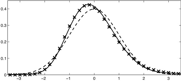
Figure 1. The probability density function of the Wigner delay time scaled and centered to have zero mean and unit variance. The crosses are a Monte-Carlo simulation for $n=20$ and $\beta=1$, computed using the $\beta$-Laguerre tri-diagonal ensemble with $100,000$ samples. The solid line is a five cumulant Edgeworth approximation, computed from our recurrence relations, and yielding remarkable agreement. The dashed line depicts the limiting Gaussian as $n\to\infty$.

By equating the first few powers of $z$ in the ODE (2.20), we obtain non-perturbative (finite-$n$) results for the lower order cumulants:

(2.32a) $$K^{(\beta)}_{1} =\frac{\beta}{2}\frac{n}{\omega}=1,$$

(2.32b) $$K^{(\beta)}_{2} =\left(\frac{\beta}{2}\right)^{2}\frac{n(2\omega+\beta n)}{\omega^{2}(2\omega+\beta)(\omega-1)}=\frac{4}{(n+1)(n\beta-2)},$$

$$K^{(\beta)}_{3} =\left(\frac{\beta}{2}\right)^{3}\frac{4n(2\omega+n\beta)(\omega+n\beta)}{\omega^{3}(2\omega+\beta)(\omega+\beta)(\omega-1)(\omega-2)}$$

(2.32c) $$=\frac{96}{(n+1)(n+2)(n\beta-2)(n\beta-4)},$$

where $\omega=b-2-\beta(n-1)$. Our formula (2.32b) for the variance can be extracted from earlier results in the quantum transport literature [40, 39]. When $\beta=2$, it has also appeared in the context of wireless communications [62]. To the best of our knowledge, our formula (2.32c) for the third cumulant has never appeared in the literature before.

From Eq. (2.32b) it follows immediately that the variance of the Wigner delay time satisfies the asymptotic formula

(2.33) $$n^{2}K^{(\beta)}_{2}\sim\frac{4}{\beta}+\frac{4}{\beta n}\left(\frac{2}{\beta}-1\right)+O(n^{-2})\quad n\to\infty.$$

In the literature on semiclassical approaches to this problem, it is a simple matter to see that Eq. (2.33) in addition to the first seven terms in the asymptotic expansion of Eq. (2.32b) are in agreement with semiclassical computations in [54]. We believe it would be important to go further and obtain a semiclassical derivation of (2.32b) to all orders in $1/n$.

Beyond the third cumulant, the exact results become more complicated. We conclude our discussion of the time delay by giving the explicit expressions for the fourth cumulant in each symmetry class:

(2.34a) $$K^{(1)}_{4} =\frac{96(53n^{2}-68n-156)}{(n-4)(n+1)^{2}(n-2)^{2}(n+3)(n+2)(n-6)},$$

(2.34b) $$K^{(4)}_{4} =\frac{12(53n^{2}+34n-39)}{(n+2)(n+1)^{2}(n-1)(2n-3)(2n-1)^{2}(n+3)},$$

(2.34c) $$K^{(2)}_{4} =\frac{12(53n^{2}-77)}{(n^{2}-1)^{2}(n^{2}-4)(n^{2}-9)}.$$

The higher order cumulants $K^{(\beta)}_{j}$ with $j>4$ can be obtained systematically from our recurrence relations in Sec. 6, valid for any $n$ and any $\beta\in\{1,2,4\}$. In Fig. 1 we used this to calculate an Edgeworth series approximation to the exact distribution of $\tau_{W}$ for $n=20$ and $\beta=1$. It shows that the cumulants accurately reproduce the deviations from the limiting Gaussian as $n\to\infty$. Very recently, such deviations were also successfully described using the Couloumb gas approach [82].

2.3. Shot Noise when $n=m$ and $\beta=2$

We end the overview of our results by discussing two interesting properties of the shot noise for symmetry classes with $\beta=2$ that have remained unnoticed in the quantum transport literature. These are immediate consequences of the definition of the moment generating function (2.1) and of previous results from Witte et al. [90] and Forrester [36].

When the two scattering leads in the cavity support the same number of quantum channels, i.e. $n=m$, the description of shot noise simplifies considerably if $\beta=2$ because $\alpha=0$. We first discuss how the moment generating function can be expressed in terms of the Painlevé V transcendent; then, we point out an interesting identity between the probability distributions of the shot noise and the conductance.

2.3.1. Shot Noise and Painlevé V

It is well known that gap probabilities in ensembles with $\beta=2$ are related to Painlevé transcendents. In particular for the Gaussian Unitary Ensemble we have the following.

Proposition 2.14 (Witte, Forrester and Cosgrove [90]).

Consider the Gaussian Unitary Ensemble of random matrices and let $E_{2}(w)$ be the probability that the interval $(-\infty,-w)\cup(w,\infty)$ contains no eigenvalues. Then,

(2.35) $$R(w):=\frac{1}{2}\frac{d}{dw}\log E_{2}(w).$$

satisfies the non-linear ODE

(2.36) $$wR^{\prime\prime}+2R^{\prime}=2w(w-h)-2h\sqrt{(R+wR^{\prime})^{2}-4w^{2}(w-h)R-2nw^{2}(s-h)^{2}},$$

where

(2.37) $$h=\sqrt{w^{2}-2R^{\prime}}.$$

The function $R(w)$ can be expressed in terms of Painlevé V transcendents with appropriate boundary conditions [90].

It turns out that the gap probability $E_{2}(w)$ is directly related to the moment generating function of the shot noise. More precisely, we have

(2.38) $$E_{2}(w)=Ce^{-w^{2}n}(2w)^{n^{2}}\mathcal{M}_{n}^{(2)}(0,-4w^{2}),$$

where $C$ is a multiplicative constant that does not affect the definition (2.35). The identity (2.38) follows from

(2.39) $$\begin{split}\mathcal{M}_{n}^{(2)}(0,-w)&=\frac{1}{c^{(2)}_{n}}\int_{[0,1]^{n}}\prod_{j=1}^{n}e^{wT_{j}(1-T_{j})}\prod_{1\leq j<k\leq n}\left\lvert T_{k}-T_{j}\right\rvert^{2}dT_{1}\dotsm dT_{n}\\ &=\frac{e^{wn/4}w^{-n^{2}/2}}{c^{(2)}_{n}}\int_{[-\sqrt{w}/2,\sqrt{w}/2]^{n}}\prod_{j=1}^{n}e^{-T_{j}^{2}}\prod_{1\leq j<k\leq n}\left\lvert T_{k}-T_{j}\right\rvert^{2}dT_{1}\dotsm dT_{n},\end{split}$$

which is obtained by completing the square in the exponential and by changing variables.

2.3.2. Shot Noise and Conductance

There is a fascinating relation between the distributions of the shot noise and the conductance in non-superconductive and superconductive quantum dots, respectively.

Proposition 2.15.

Let $P_{n}^{(2,0)}$, $G^{(2,-1)}_{N_{1}}$ and $G^{(2,1)}_{N_{2}}$ denote the random variables defined in (1.4), where

(2.40) $$N_{1}:=\left\lfloor\frac{n+1}{2}\right\rfloor\quad\text{and}\quad N_{2}:=\biggl{\lfloor}\frac{n}{2}\biggr{\rfloor}.$$

The subscripts refer to the number of variables in the j.p.d.f. (1.7), while the superscripts emphasize its dependence on the parameters $(\beta,\delta)$. In addition we assume that $\alpha=0$. We have

(2.41) $$P_{n}^{(2,0)}\overset{d}{\equiv}\frac{G^{(2,-1)}_{N_{1}}+G^{(2,1)}_{N_{2}}}{4},$$

where the notation $\overset{d}{\equiv}$ denotes equivalence in distribution.

Proof.

The proof follows from a result of Forrester [36], who exploited the symmetry of the integration interval in the right-hand side of (2.39), together with the evenness of the Gaussian weight. He thus obtained the identity

(2.42) $$\begin{split}\mathcal{M}_{n}^{(2)}(0,-w)&=\frac{e^{wn/4}}{c_{n}^{(2)}}\int_{[0,1]^{N_{1}}}\prod_{j=1}^{N_{1}}T_{j}^{-1/2}e^{-wT_{j}/4}\prod_{1\leq j<k\leq N_{1}}\left\lvert T_{k}-T_{j}\right\rvert^{2}dT_{1}\dotsm dT_{N_{1}}\\ &\quad\times\int_{[0,1]^{N_{2}}}\prod_{j=1}^{N_{2}}T_{j}^{1/2}e^{-wT_{j}/4}\prod_{1\leq j<k\leq N_{2}}\left\lvert T_{k}-T_{j}\right\rvert^{2}dT_{1}\dotsm dT_{N_{2}}.\end{split}$$

Changing the variables $T_{j}\to 1-T_{j}$, and scaling $w\to 4w$ gives

(2.43) $$\mathcal{M}_{n}^{(2)}(0,-4w)=\mathcal{M}^{(2)}_{N_{1}}(-w)\biggr{\rvert}_{\delta=-1}\mathcal{M}^{(2)}_{N_{2}}(-w)\biggr{\rvert}_{\delta=1}.$$

Finally, Eq. (2.41) follows from the convolution theorem. ∎

When $(\beta,\delta)=(2,-1)$, then the compact symmetric space of the scattering matrix $S$ is of symmetry type DIII; this means that $S$ is orthogonal and self-dual. When $(\beta,\delta)=(2,1)$ the symmetric space is of symmetry type CI; in this case $S$ is symplectic and symmetric. Note that matrices of symmetry type DIII are real, while matrices of symmetry type CI have quaternion elements. In both instances time-reversal is preserved. The Landauer-Büttiker scattering matrix $S$ of the system on the right-hand side belongs to the CUE; thus, interestingly, time-reversal is broken on the left-hand side of Eq. (2.41) but not on the right-hand side.

From a computational perspective, we note that the right-hand side of (2.41) is far more amenable to calculation than the left-hand side. As we shall see in Sec. 4, the cumulants of $G^{(2,-1)}_{N_{1}}$ and $G^{(2,1)}_{N_{2}}$ can be determined from the one-dimensional difference equation (4.6), while to obtain the cumulants of the shot noise we have to study the partial recurrence relation (4.16).

3. Integrable Systems and Moment Generating Functions

We can associate to a scattering observable, such as the Landauer conductance or the Wigner delay time, a moment generating function whose integral representation is a partition function of one of the orthogonal, unitary or symplectic ensembles of random matrices, depending on whether $\beta=1$, $\beta=2$ or $\beta=4$. In this section we describe the general theory that provides a link between such partition functions and certain integrable non-linear differential equations.

3.1. Matrix Integrals, $\tau$-Functions and Integrable Hierarchies

Fundamental to our approach is the connection between matrix integrals and exactly solvable models, as established in a variety of papers, e.g., [66, 42, 2, 5, 83, 3]. These works focus principally on the case $\beta=2$ and obtain relations to the Toda lattice and KP hierarchies. In contrast, the existence of integrable structures related to the $\beta=1,4$ matrix integrals [6, 4, 8] has received comparatively little attention.

The starting point for establishing the relationship with integrable hierarchies is the deformed integral

(3.1) $$\tau_{n}^{(\beta)}(\mathbf{t}):=\frac{1}{n!}\int_{[A,B]^{n}}\prod_{j=1}^{n}\rho(x_{j})\exp\left(\sum_{i=1}^{\infty}t_{i}x_{j}^{i}\right)\prod_{1\leq j<k\leq n}\left\lvert x_{k}-x_{j}\right\rvert^{\beta}dx_{1}\dotsm dx_{n},$$

defined by introducing an infinite sequence of time variables $\mathbf{t}=(t_{1},t_{2},t_{3},\ldots)$ into the integrands of Eqs. (2.1) and (2.15). For the mixed moment generating function of conductance and shot noise, $[A,B]=[0,1]$ and the weight function is

(3.2) $$\rho_{z,w}(T)=T^{\alpha}(1-T)^{\delta/2}e^{-zT-wT(1-T)}.$$

For the Wigner delay time, we have $[A,B]=[0,\infty)$ and

(3.3) $$\rho_{z}(\lambda)=\lambda^{-b}\exp\left(-\frac{1}{\lambda}+z\lambda\right),$$

where $z<0$. In the theory of integrable systems the integral (3.1) is known as a $\tau$-function.

When $\beta=2$ the integral (3.1) simplifies considerably and can be written as a Hankel determinant, which can be studied using orthogonal polynomials. We have

(3.4) $$\tau^{(2)}_{n}(\mathbf{t})=\det\left(\int_{A}^{B}x^{i+j}\rho(x)e^{\sum_{i=1}^{\infty}t_{i}x^{i}}dx\right)_{0\leq i,j\leq n-1}.$$

When $\beta=1$, however, no such nice structure exists. In this case, for even $n$ the $\tau$-function (3.1) becomes the Pfaffian of a skew symmetric matrix (the square root of its determinant). Namely, (see, e.g., [63])

(3.5) $$\tau_{n}^{(1)}(\mathbf{t})=\operatorname{Pf}\left(\frac{1}{2}\int_{A}^{B}\int_{A}^{B}y^{k}x^{l}\operatorname{sgn}(y-x)e^{\sum_{i=1}^{\infty}t_{i}(y^{i}+x^{i})}\rho(y)\rho(x)dydx\right)_{0\leq k,l\leq n-1}.$$

Although we shall restrict our attention to the weights defined in (3.2) and (3.3), the identity (3.5) holds independently of these choices or the deformation parameters $\mathbf{t}$. Formula (3.5) is based on an identity of de Bruijn for integrating determinants:

(3.6) $$\frac{1}{n!}\int_{[A,B]^{n}}\det\left(F_{i}(y_{1}),G_{i}(y_{1}),\dotsc,F_{i}(y_{n}),G_{i}(y_{n})\right)_{0\leq i\leq 2n-1}dy_{1}\dotsm dy_{n}\\ =\operatorname{Pf}\left(\int_{A}^{B}(G_{i}(y)F_{j}(y)-F_{i}(y)G_{j}(y))dy\right)_{0\leq i,j\leq 2n-1},$$

where $F_{i}$ and $G_{i}$, $i=0,\dotsc,n-1$, are two sets of integrable functions. In the left-hand side of (3.6), the commas separate columns and the index $i$ labels the rows.

By studying the evolution of the moment matrix (3.5) in the extended $\mathbf{t}$-space, Adler and van Moerbeke [6, 8, 4] discovered a bi-linear identity that applies to $\tau$-functions that can be expressed as Pfaffians:

(3.7) $$\oint_{\mathcal{C}_{\infty}}\tau^{(1)}_{n}\left(\mathbf{t}-\left[\xi^{-1}\right]\right)\tau^{(1)}_{m+2}\left(\mathbf{t}^{\prime}+\left[\xi^{-1}\right]\right)e^{\sum_{i=1}^{\infty}(t_{i}-t_{i}^{\prime})\xi^{i}}\xi^{n-m-2}\frac{d\xi}{2\pi i}\\ =-\oint_{\mathcal{C}_{0}}\tau^{(1)}_{m}(\mathbf{t}^{\prime}-[\xi])\tau^{(1)}_{n+2}(\mathbf{t}+[\xi])e^{\sum_{i=1}^{\infty}(t_{i}^{\prime}-t_{i})\xi^{-i}}\xi^{n-m}\frac{d\xi}{2\pi i},$$

where $n$ and $m$ are even, and $\mathcal{C}_{\infty}$ or $\mathcal{C}_{0}$ are small circles in the complex plane enclosing the point $\xi=\infty$ and $\xi=0$, respectively. The notation $[\xi]$ refers to the infinite vector $(\xi,\xi^{2}/2,\xi^{3}/3,\ldots)$.

The identity (3.7) can be used to generate an infinite sequence of integrable hierarchies of PDEs involving $\tau^{(1)}_{n}(\mathbf{t})$. Evaluating the residues on both sides of (3.7) and expanding up to terms linear in $(\mathbf{t}-\mathbf{t}^{\prime})$, one obtains a hierarchy of PDEs known as the Pfaff-KP hierarchy; its first non-trivial member is the Pfaff-KP equation:

(3.8) $$\left(\frac{\partial^{4}}{\partial t_{1}^{4}}+3\frac{\partial^{2}}{\partial t_{2}^{2}}-4\frac{\partial^{2}}{\partial t_{1}\partial t_{3}}\right)\log\tau^{(1)}_{n}+6\left(\frac{\partial^{2}}{\partial t_{1}^{2}}\log\tau^{(1)}_{n}\right)^{2}=12\frac{\tau^{(1)}_{n-2}\tau^{(1)}_{n+2}}{\bigl{(}\tau^{(1)}_{n}\bigr{)}^{2}}.$$

When Eq. (3.8) was introduced in RMT, it was used to characterize gap formation probabilities in orthogonal and symplectic ensembles [6]. To the best of our knowledge, this article is the first to apply (3.8) in a physical context for over a decade.

A similar discussion holds when $\beta=4$. One can show that $\tau^{(4)}_{n}(2\mathbf{t})$ satisfies the same equation as $\tau^{(1)}_{n}(\mathbf{t})$, except for one small difference: in the right-hand side the sub-indices $n\pm 2$ are replaced by $n\pm 1$ and there is no parity restriction on $n$.

Although our emphasis is on the $\beta=1,4$ ensembles, we point out that when $\beta=2$ there is a simpler and more widely known analogue of (3.8) usually referred to as the KP equation:

(3.9) $$\left(\frac{\partial^{4}}{\partial t_{1}^{4}}+3\frac{\partial^{2}}{\partial t_{2}^{2}}-4\frac{\partial^{2}}{\partial t_{1}\partial t_{3}}\right)\log\tau^{(2)}_{n}+6\left(\frac{\partial^{2}}{\partial t_{1}^{2}}\log\tau^{(2)}_{n}\right)^{2}=0,$$

which is the first member of the KP hierarchy.

It is worth emphasizing that the right-hand side of Eq. (3.8) is not zero as well as containing $\tau^{(1)}_{n\pm 2}(\mathbf{t})$ ($\beta=1$) or $\tau^{(4)}_{n\pm 1}(2\mathbf{t})$ ($\beta=4$). This constitutes an additional complication compared to the symmetry classes with $\beta=2$.

Equation (3.8) is the starting point to obtain the differential equations in Theorems 2.4, 2.5 and 2.9; in turn such differential equations lead to recurrence relations for the cumulants. Deriving these differential equations requires a combination of techniques pioneered by Adler and van Moerbeke [6]. More precisely we need extra information on the properties of $\tau$-functions that is provided by the fact that (3.1) satisfies the Virasoro constraints. These are an infinite sequence of linear differential equations with a specific algebraic structure, which we discuss next.

3.2. Virasoro Constraints and $\beta$-Integrals

The Virasoro constraints were first applied to unitary matrix models ($\beta=2$) in the context of string theory [66, 42]. In the unitary case, Osipov and Kanzieper [73] were the first to apply these techniques to quantum transport and used (3.9) to derive a PDE satisfied by $\log\mathcal{M}_{n}^{(2)}(z,w)$. The fact that the Virasoro constraints apply for general $\beta>0$ appears not to have been applied to problems in quantum transport until now.

The integrals (3.1) are well-defined for any real $\beta>0$. Usually, when we want to emphasize this property, we refer to them as $\beta$-integrals. The Virasoro constraints we need follow from a particular change of integration variables. More generally, let $f(x)$ and $g(x)$ be real analytic in a neighbourhood of the origin and supported on an interval $[A,B]\subseteq\mathbb{R}$. In addition impose the boundary conditions

(3.10) $$V^{\prime}(x):=\frac{g(x)}{f(x)}=\frac{\sum_{i=0}^{\infty}b_{i}x^{i}}{\sum_{i=0}^{\infty}a_{i}x^{i}},\quad\lim_{x\to A,B}f(x)\rho(x)x^{k}=0,\quad\text{for all $k>0$.}$$

The $\tau$-functions (3.1) belong to the class of $\beta$-integrals with weights of the form

(3.11) $$\rho(x):=e^{-V(x)},\quad x\in[A,B]\subseteq\mathbb{R}.$$

It is straightforward to check that the boundary conditions (3.10) are satisfied by both weights (3.2) and (3.3).

Let us introduce the differential operators

$$J_{k}^{(1)} :=\begin{cases}\frac{\partial}{\partial t_{k}}&k>0,\\ \frac{1}{\beta}(-k)t_{-k}&k<0,\\ 0&k=0,\end{cases}$$

$$J_{k}^{(2)} :=\sum_{i=1}^{k-1}\frac{\partial^{2}}{\partial t_{i}\partial t_{k-i}}+\frac{2}{\beta}\sum_{i=1}^{\infty}it_{i}\frac{\partial}{\partial t_{i+k}},$$

where $t_{1},\dots,t_{k}$ are the first $k$ elements of the infinite vector $\mathbf{t}=(t_{1},t_{2},t_{3},\dotsc)$. Define

(3.12a) $$\mathbb{J}_{k,n}^{(1)} :=J_{k}^{(1)}+n\delta_{0,k},$$

(3.12b) $$\mathbb{J}_{k,n}^{(2)} :=\left(\frac{\beta}{2}\right)J_{k}^{(2)}+\Biggl{(}n\beta+(k+1)\left(1-\frac{\beta}{2}\right)\Biggr{)}J_{k}^{(1)}+n\left((n-1)\frac{\beta}{2}+1\right)\delta_{0,k},$$

as well as the Virasoro operators

(3.13) $$\mathcal{V}_{k}:=\sum_{i=0}^{\infty}\left(a_{i}\,\mathbb{J}_{k+i,n}^{(2)}-b_{i}\,\mathbb{J}_{k+i+1,n}^{(1)}\right),\quad k\geq-1,$$

where the parameters $a_{i}$ and $b_{i}$, $i=0,1,2,\dotsc,$ are the coefficients of the Taylor expansion of $f(x)$ and $g(x)$ defined in Eq. (3.10). Imposing the invariance of (3.1) under the transformation

(3.14) $$x_{j}\to x_{j}+\epsilon f(x_{j})x_{j}^{k+1},\quad j=1,\dotsc,n.$$

one can show that (see Appendix $5$ of [6])

(3.15) $$\mathcal{V}_{k}\tau_{n}(\mathbf{t})=0,\quad k\geq-1.$$

We shall refer to these identities as Virasoro constraints. A more abstract proof of Eq. (3.15) is based on the fact that the $\beta$-integrals (3.1) are the fixed points of vertex operators [6].

It is worth emphasizing that the differential operators (3.12) form an algebra, although this fact will not enter directly in our discussion. For all $n\in\mathbb{Z}_{+}$ the operators $\mathbb{J}^{(1)}_{k,n}$ and $\mathbb{J}^{(2)}_{k,n}$ obey a Virasoro and Heisenberg algebra

$$\left[\mathbb{J}^{(1)}_{k,n},\mathbb{J}^{(1)}_{\ell,n}\right] =\frac{k}{\beta}\delta_{k,-\ell},$$

$$\left[\mathbb{J}^{(2)}_{k,n},\mathbb{J}^{(1)}_{\ell,n}\right] =-\ell\,\mathbb{J}^{(1)}_{k+\ell,n}+c^{\prime}k(k+1)\delta_{k,-\ell},$$

$$\left[\mathbb{J}^{(2)}_{k,n},\mathbb{J}^{(2)}_{\ell,n}\right] =\left(k-\ell\right)\mathbb{J}^{(2)}_{k+\ell,n}+c\left(\frac{k^{3}-k}{12}\right)\delta_{k,-\ell}$$

with central charge

$$c=1-6\Biggl{(}\left(\frac{\beta}{2}\right)^{1/2}-\left(\frac{\beta}{2}\right)^{-1/2}\Biggr{)}^{2}\quad\text{and}\quad c^{\prime}=\frac{1}{\beta}-\frac{1}{2}.$$

3.3. Virasoro Constraints for Joint Conductance and Shot Noise

To put the theory of the matrix integrals described in Secs. 3.1 and 3.2 into our context, let us look at the $\tau$-function obtained by deforming the joint moment generating function (2.1).

Since only linear and quadratic terms in the transmission eigenvalues $T_{j}$ appear in the weight (3.2), we only need the first two Virasoro constraints. The logarithmic derivative of the weight (3.2)

$$\begin{split}\frac{f(T)}{g(T)}&=-\frac{d}{dT}\log\rho_{z,w}(T)\\ &=\frac{\alpha-(\alpha+\delta/2+z+w)T+(z+3w)T^{2}-2wT^{3}}{T(T-1)}\end{split}$$

gives the coefficients of the Taylor expansions of $f(T)$ and $g(T)$:

$$a_{0} =0, \quad a_{1} =-1, \quad a_{2} =1, \quad a_{3} =0,$$

$$b_{0} =\alpha, b_{1} =-(\alpha+\delta/2+z+w), b_{2} =z+3w, b_{3} =-2w,$$

$$a_{i} =0, b_{i} =0\quad\text{if $i>3$.}$$

The first two Virasoro operators are:

(3.16a) $$\begin{split}\mathcal{V}_{-1}&=\sum_{i=1}^{\infty}it_{i}\left(\frac{\partial}{\partial t_{i+1}}\ -\frac{\partial}{\partial t_{i}}\right)+\Bigl{(}\alpha+z+\delta/2+w+\bigl{(}n\beta+2-\beta\bigr{)}\Bigr{)}\frac{\partial}{\partial t_{1}}\\ &\quad-(z+3w)\frac{\partial}{\partial t_{2}}+2w\frac{\partial}{\partial t_{3}}-\Bigl{(}\alpha n+n((n-1)\beta/2+1)\Bigr{)}\end{split}$$

and

(3.16b) $$\begin{split}\mathcal{V}_{0}&=\sum_{i=1}^{\infty}it_{i}\left(\frac{\partial}{\partial t_{i+2}}-\frac{\partial}{\partial t_{i+1}}\right)+\frac{\beta}{2}\frac{\partial^{2}}{\partial t_{1}^{2}}-\Bigl{(}\bigl{(}n\beta+2-\beta\bigr{)}+\alpha\Bigr{)}\frac{\partial}{\partial t_{1}}\\ &\quad+\Bigl{(}\alpha+z+\delta/2+w+\bigl{(}n\beta+3-3\beta/2\bigr{)}\Bigr{)}\frac{\partial}{\partial t_{2}}\\ &\quad-(z+3w)\frac{\partial}{\partial t_{3}}+2w\frac{\partial}{\partial t_{4}}.\end{split}$$

The Virasoro operators associated to the deformation of the moment generating function of the conductance are obtained simply by setting $w=0$ in Eqs. (3.16a) and (3.16b).

4. Conductance and Shot Noise for Finite-$n$

The Virasoro constraints allow us to evaluate the Pfaff-KP equation (3.8) and the KP equation (3.9) at $\mathbf{t}=0$. This gives the differential equations (2.11) and (2.13), thus proving Theorems 2.4 and 2.5. Then, by inserting the series expansions (2.2) into these differential equations we obtain recurrence relations, which allow both non-perturbative and asymptotic analysis of the cumulants as $n\to\infty$.

4.1. Differential-Difference Equations: the Conductance

As discussed in Sec 2.1 the cumulants of the conductance $\kappa_{l}^{(\beta)}$ provide the initial conditions for the recurrence relation for the mixed cumulants $\kappa_{l,k}^{(\beta)}$. Therefore, we shall start with the proof of Theorem 2.5.

Let us write down the $\tau$-function associated to the weight (3.2) explicitly

(4.1) $$\begin{split}\tau_{n}(\mathbf{t};z,w)&:=\frac{1}{n!}\int_{[0,1]^{n}}\prod_{j=1}^{n}T_{j}^{\alpha}(1-T_{j})^{\delta/2}\\ &\quad\times\exp\left(-zT_{j}-wT_{j}(1-T_{j})+\sum_{i=1}^{\infty}T_{j}^{i}t_{i}\right)\prod_{1\leq j<k\leq n}\left\lvert T_{k}-T_{j}\right\rvert^{\beta}dT_{1}\dotsm T_{n}.\end{split}$$

We now study the $\tau$-function $\tau_{n}(\mathbf{t};z):=\tau_{n}(\mathbf{t};z,0)$ as well as the moment generating function

(4.2) $$\mathcal{M}_{n}^{(\beta)}(z):=\frac{n!}{c_{n}^{(\beta)}}\tau_{n}^{(\beta)}(\mathbf{t};z)\biggr{\rvert}_{\mathbf{t}=\mathbf{0}}.$$

First note that the definition (4.1) and (3.1) imply the relation

(4.3) $$\frac{\partial}{\partial t_{1}}\tau^{(\beta)}_{n}(\mathbf{t};z)=-\frac{\partial}{\partial z}\tau^{(\beta)}_{n}(\mathbf{t};z).$$

Eqs. (4.2) and (4.3) provide the projections at $\mathbf{t}=\mathbf{0}$ of the right-hand side of (3.8) (for both $\beta=1$ and $\beta=4$) as well as of the partial derivatives with respect to $t_{1}$ in the left-hand side. Therefore, in order to complete the proof of Theorem 2.5 we need to express the partial derivatives

(4.4) $$\frac{\partial^{2}}{\partial t_{2}^{2}}\log\tau^{(\beta)}_{n}(\mathbf{t};z)\biggr{\rvert}_{\mathbf{t}=\mathbf{0}}\quad\text{and}\quad\frac{\partial^{2}}{\partial t_{1}\partial t_{3}}\log\tau^{(\beta)}_{n}(\mathbf{t};z)\biggr{\rvert}_{\mathbf{t}=\mathbf{0}}$$

in terms of the derivatives of $\sigma_{n}^{(\beta)}(z)=\log\mathcal{M}^{(\beta)}_{n}(z)$. This is a standard calculation involving the Virasoro operators (3.16a) and (3.16b), whose details are provided in Appendix A.

4.2. Non-Perturbative Recurrence Relation for the Cumulants of the Conductance

The ODE (2.13) combined with the Taylor expansion

(4.5) $$\sigma^{(\beta)}_{n}(z):=\sum_{l=1}^{\infty}\frac{(-1)^{l}\kappa_{l}^{(\beta)}}{l!}z^{l}$$

provides a non-perturbative recurrence relation that the cumulants $\kappa_{l}^{(\beta)}$ satisfy. In Sec. 5 we shall study its asymptotic limit as $n\to\infty$.

Lemma 4.1.

The cumulants $\kappa_{l}^{(\beta)}$ satisfy the recurrence relation

(4.6) $$A(l)\kappa^{(\beta)}_{l+1}+\eta_{1,4}^{(\beta)}\sum_{i=0}^{l-1}\binom{l}{i}\kappa^{(\beta)}_{i+1}\kappa^{(\beta)}_{l-i}B(i,l)-l(2l-1)(\alpha-\delta/2+\beta n)\kappa^{(\beta)}_{l}\\ -l(l-1)(l-2)\kappa^{(\beta)}_{l-1}=(12b_{n}^{(\beta)}/\beta)l(l-1)(l-2)\mu^{(\beta)}_{l-3},\quad l\geq 3$$

with initial conditions

(4.7a) $$\kappa^{(\beta)}_{1} =\frac{n\bigl{(}\alpha+1+\beta(n-1)/2\bigr{)}}{\alpha+\delta/2+2+\beta(n-1)},$$

(4.7b) $$\kappa^{(\beta)}_{2} =\frac{1}{4}\frac{n\bigl{(}2\alpha+2+\beta(n-1)\bigr{)}\bigl{(}\delta+2+\beta(n-1)\bigr{)}}{\bigl{(}\alpha+\delta/2+2+\beta(n-1)\bigr{)}^{2}\bigl{(}\alpha+\delta/2+3+\beta(n-1)\bigr{)}}$$

$$\quad\times\frac{\bigl{(}\delta+2\alpha+4+\beta(n-2)\bigr{)}}{\bigl{(}2\alpha+\delta+4+\beta(2n-3)\bigr{)}},$$

(4.7c) $$\kappa^{(\beta)}_{3} =\frac{2\kappa_{2}^{(\beta)}(\delta/2-\alpha+2\beta\kappa^{(\beta)}_{1}-\beta n)}{\bigl{(}\alpha+\delta/2+4+\beta(n-1)\bigr{)}\bigl{(}\alpha+\delta/2+2+\beta(n-2)\bigr{)}}.$$

The parameter $b_{n}^{(\beta)}$ was defined in Eq. (2.9) and the coefficients $A(l)$ and $B(i,l)$ are polynomials in $i$ and $l$:

(4.8a) $$A(l) :=\eta^{(\beta)}_{1,4}l(l-1)(l-2)+\beta l(2l-1)-(6-3\beta)(\alpha+\delta/2+\beta n+2-\beta)l$$

$$\quad\;-(\alpha+\delta/2+\beta n)(\alpha+\delta/2+\beta n+2-\beta)(l+1),$$

(4.8b) $$B(i,l) :=(2-\chi_{1,2}^{(\beta)})(l-i)\Bigl{(}(l-i)(6i-2)+3\Bigr{)}+(\chi_{1,2}^{(\beta)}-1)(l-i)^{2}(6i+2),$$

where

$$\chi_{1,2}^{(\beta)}:=\begin{cases}1&\text{if $\beta=1,4$,}\\ 2&\text{if $\beta=2$.}\end{cases}$$

The coefficients $\mu_{l}^{(\beta)}$, $l=0,1,2\dotsc$ are the “reduced moments”, which can be obtained from the recurrence relation

(4.9) $$\mu^{(\beta)}_{l}=\sum_{j=0}^{l-1}\binom{l-1}{j}r^{(\beta)}_{l-j}\mu^{(\beta)}_{j},\qquad l=1,2,\dotsc,$$

where

(4.10) $$r^{(\beta)}_{l}:=\kappa^{(\beta)}_{l}\Bigr{\rvert}_{n\to n-i(\beta)}+\kappa^{(\beta)}_{l}\Bigr{\rvert}_{n\to n+i(\beta)}-2\kappa^{(\beta)}_{l},$$

and by convention we have set $\mu_{0}=1$. The integer $i(\beta)$ was introduced in Eq. (2.10).

This lemma can be proved by inserting the expansion (4.5) into the ODE (2.13) and performing straightforward, although tedious, calculations. The initial conditions (4.7) are obtained by equating the coefficients of the first three powers of $z$ on both sides of the ODE. The right-hand side of Eq. (2.13) contributes only for powers $z^{l}$ such that $l>3$ and is expanded using the identity

(4.11) $$\exp\left(\sum_{l=1}^{\infty}\frac{r^{(\beta)}_{l}z^{l}}{l!}\right)=1+\sum_{l=1}^{\infty}\frac{\mu^{(\beta)}_{l}z^{l}}{l!}.$$

Since the coefficient $\mu^{(\beta)}_{l-3}$ on the right-hand side of (4.6) involves only the first $l-3$ reduced cumulants, the difference equation (4.6) and the initial conditions (4.7) define the cumulants of conductance for systems with $\beta=1,4$ uniquely. It also presents an efficient algorithm for their computation.

Remark 4.2.

Formulae (4.7) generalise previous results [78, 81, 79, 51] to the symmetry classes $\delta\neq 0$. The right-hand side of the differential equation (2.13) does not contribute to the recurrence relation until one equates the coefficients of the third power of $z$. In other words, it does not contribute to the first three cumulants. It is possible to verify using only the Virasoro constraints that the formulae in (4.7) are valid for arbitrary $\beta>0$.

Remark 4.3.

By setting $l=3$ in (4.6) we obtain exact formulae for the fourth cumulant of conductance in terms of the first three. For example, when $\beta=1,2$ we have

(4.12a) $$\kappa^{(1)}_{4} =3\left(\frac{-2\kappa^{(1)}_{2}+10\kappa^{(1)}_{1}\kappa^{(1)}_{3}+22\bigl{(}\kappa^{(1)}_{2}\bigr{)}^{2}+5\kappa^{(1)}_{3}(\delta/2-\alpha-n)-24b^{(1)}_{n}}{(\alpha+\delta/2+n+4)(4\alpha+2\delta+4n-3)}\right),$$

(4.12b) $$\kappa^{(2)}_{4} =\frac{3}{4}\left(\frac{-2\kappa^{(2)}_{2}+20\kappa^{(2)}_{1}\kappa^{(2)}_{3}+32\bigl{(}\kappa^{(2)}_{2}\bigr{)}^{2}+5\kappa^{(2)}_{3}(\delta/2-\alpha-2n)}{(\alpha+\delta/2+2n)^{2}-9}\right).$$

When $\beta=1$, formula (4.12a) involves the constant $b^{(1)}_{n}$, whose value is given explicitly in Eq. (B.1a). At first sight it seems that both cumulants (4.12a) and (4.12b) should be of order $O(n^{-2})$ as $n\to\infty$, since $\kappa^{(\beta)}_{j}$ is $O(n^{2-j})$ for $j=1,2$ and $\kappa^{(\beta)}_{3}$ is $O(n^{-3})$. A closer inspection reveals that (4.12b) contains mutually cancelling terms which lead to $\kappa^{(2)}_{4}$ being $O(n^{-4})$. When $\beta=1$ these cancellations are suppressed by the constant $b^{(1)}_{n}$ causing $\kappa^{(1)}_{4}=O(n^{-3})$. From the recursion relation (4.6), one easily sees that this “staircase” effect persists in all higher cumulants of the conductance. When $\beta=4$ we observe a similar behaviour to the case $\beta=1$.

4.3. Differential-Difference Equation: Joint Conductance and Shot Noise

The aim of the this subsection is to prove Theorem 2.4 by deriving the non-linear PDE (2.11). The strategy, as in the proof of Theorem 2.5, is to combine the Pfaff-KP equation (3.8) satisfied by the $\tau$-function (4.1) with the Virasoro constraints.

First observe the trivial identities

(4.13a) $$\tau^{(\beta)}_{n}(\mathbf{t};z,w)\Bigr{\rvert}_{\mathbf{t}=0} =\frac{c^{(\beta)}_{n}}{n!}\mathcal{M}^{(\beta)}_{n}(z,w),$$

(4.13b) $$\frac{\partial}{\partial t_{1}}\tau^{(\beta)}_{n}(\mathbf{t};z,w) =-\frac{\partial}{\partial z}\tau^{(\beta)}_{n}(\mathbf{t};z,w),$$

(4.13c) $$\frac{\partial}{\partial t_{2}}\tau^{(\beta)}_{n}(\mathbf{t};z,w) =\frac{\partial}{\partial w}\tau^{(\beta)}_{n}(\mathbf{t};z,w)-\frac{\partial}{\partial z}\tau^{(\beta)}_{n}(\mathbf{t};z,w).$$

Therefore, the partial derivatives of any order with respect to $t_{1}$ and $t_{2}$ of $\tau_{n}^{(\beta)}(\mathbf{t};z,w)$ can be expressed in terms of the partial derivatives of $\mathcal{M}^{(\beta)}_{n}(z,w)$. It follows that the only missing term in the Pfaff-KP equation (3.8) is

(4.14) $$\frac{\partial^{2}}{\partial t_{1}\partial t_{3}}\log\tau^{(\beta)}_{n}(\mathbf{t},z,w)\biggr{\rvert}_{\mathbf{t}=0}.$$

Writing the constraint (3.16a) in terms of $\log\tau_{n}(\mathbf{t},z,w)$ and taking the derivative with respect to $t_{1}$, the projection at $\mathbf{t}=\mathbf{0}$ yields the relation

(4.15) $$\left(\frac{\partial}{\partial t_{2}}-\frac{\partial}{\partial t_{1}}+(\alpha+\delta/2+z+w+n\beta+2-\beta)\frac{\partial^{2}}{\partial t_{1}^{2}}\right.\\ \left.\left.-(z+3w)\frac{\partial^{2}}{\partial t_{1}\partial t_{2}}+2w\frac{\partial^{2}}{\partial t_{1}\partial t_{3}}\right)\log\tau(\mathbf{t};z,w)\right\rvert_{\mathbf{t}=0}=0.$$

Using the relations (4.13) we can solve this equation for (4.14), which can then be written in terms of the derivatives of $\mathcal{M}_{n}^{(\beta)}(z,w)$. Eventually, after some algebra, we obtain the PDE (2.11).

4.4. Non-Perturbative Recurrence Relation for the Joint Cumulants

The last result that we need in order to pursue an asymptotic analysis of the joint cumulants of conductance and shot noise is the following.

Lemma 4.4.

The cumulants of the joint probability density function of conductance and shot noise obey the recurrence relation

(4.16) $$k(\eta_{1,4}^{(\beta)}\kappa^{(\beta)}_{l+4,k-1}-\kappa^{(\beta)}_{l+2,k-1})-2(\alpha+\delta/2+n\beta+2-\beta)\kappa^{(\beta)}_{l+2,k}+(2l+3k+2)\kappa^{(\beta)}_{l,k+1}\\ +6\eta_{1,4}^{(\beta)}k\sum_{i=0}^{k-1}\binom{k-1}{i}\sum_{j=0}^{l}\binom{l}{j}\kappa^{(\beta)}_{j+2,i}\kappa^{(\beta)}_{l-j+2,k-i-1}=\frac{12b^{(\beta)}_{n}}{\beta}k\mu^{(\beta)}_{l,k-1}$$

with boundary conditions $\left(\kappa_{l,0}^{(\beta)}\right)_{l=1}^{\infty}=\left(\kappa_{l}^{(\beta)}\right)_{l=1}^{\infty}$, which are the solutions of the difference equation (4.6). The coefficients $\mu_{l,k}^{(\beta)}$ are defined by the recurrence relation

(4.17) $$\mu^{(\beta)}_{l,k}=\sum_{i=0}^{k-1}\binom{k-1}{i}\sum_{j=0}^{l}\binom{l}{j}r^{(\beta)}_{l-j,k-i}\mu^{(\beta)}_{j,i}$$

with boundary conditions $\left(\mu_{l,0}^{(\beta)}\right)_{l=1}^{\infty}=\left(\mu_{l}^{(\beta)}\right)_{l=1}^{\infty}$ given by the solution of Eq. (4.9). The coefficients $r_{l,k}^{(\beta)}$ are the “reduced joint cumulants”

(4.18) $$r^{(\beta)}_{l,k}:=\kappa^{(\beta)}_{l,k}\Bigr{\rvert}_{n\to n-i(\beta)}+\kappa^{(\beta)}_{l,k}\Bigr{\rvert}_{n\to n+i(\beta)}-2\kappa^{(\beta)}_{l,k}.$$

The parameters $\eta_{1,4}^{(\beta)}$, $i(\beta)$ and $b_{n}^{(\beta)}$ are the same that appeared in Theorem 2.4 and were defined in Eqs. (2.9) and (2.10).

The proof is analogous to that of Lemma 4.1 provided the expansion (4.5) is replaced by (2.2), the ODE (2.13) by the PDE (2.11) and Eq. (4.11) by

$$\exp\left(\sum_{l=0}^{\infty}\sum_{k=0}^{\infty}\frac{r^{(\beta)}_{l,k}z^{l}w^{k}}{l!k!}\right)=1+\sum_{l=1}^{\infty}\sum_{k=0}^{\infty}\frac{\mu^{(\beta)}_{l,k}z^{l}w^{k}}{l!k!}.$$

Remark 4.5.

Setting $k=0$ in (4.16) leads to the relation

(4.19) $$(l+1)\kappa^{(\beta)}_{l,1}=(\alpha+\delta/2+n\beta+2-\beta)\kappa^{(\beta)}_{l+2,0},$$

which holds for $\beta\in\{1,2,4\}$. For example, setting $l=0$ and using (4.7b) gives an exact result for the average shot noise:

$$\kappa^{(\beta)}_{0,1}=\frac{1}{4}\frac{n\bigl{(}2\alpha+2+\beta(n-1)\bigr{)}\bigl{(}\delta+2+\beta(n-1)\bigr{)}\bigl{(}2\alpha+\delta+4+\beta(n-2)\bigr{)}}{\bigl{(}\alpha+\delta/2+2+\beta(n-1)\bigr{)}\bigl{(}\alpha+\delta/2+3+\beta(n-1)\bigr{)}\bigl{(}2\alpha+\delta+4+\beta(2n-3)\bigr{)}}.$$

Instead, setting $l=1$ shows that the covariance between conductance and shot noise is related in a very simple way to the third cumulant of the conductance given in Eq. (4.7c). When $\beta=2$ and $\alpha=\delta=0$ formula (4.19) was derived for all $l>1$ in [73]. Since when $k=0$ the right-hand side of the recurrence relation (4.16) does not contribute, we conjecture that (4.19) holds not only for $\beta\in\{1,2,4\}$, but also for any real $\beta>0$.

Remark 4.6.

For convenience, in Table 1 we list the first few values of the sequence $\left(\mu^{(\beta)}_{l,k}\right)_{l,k=0}^{\infty}$ appearing on the right hand side of (4.6). They are expressed in terms of the reduced joint cumulants $r^{(\beta)}_{l,k}$, defined in Eq. (4.18). For ease of notation we have dropped the superscript $(\beta)$ from the formulae in the table. Interchanging $l$ and $k$ in $\mu^{{(\beta)}}_{l,k}$ leads to the same expressions but with the indices of $r^{(\beta)}_{i,j}$ interchanged.

Table 1. The first few mixed reduced cumulants

l	k	$\mu_{l,k}$
$0$	$0$	1
$1$	$0$	$r_{1,0}$
$1$	$1$	$r_{0,1}r_{1,0}+r_{1,1}$
$2$	$0$	$r_{2,0}+r_{1,0}^{2}$
$2$	$1$	$r_{2,1}+2r_{1,0}r_{1,1}+r_{0,1}r_{2,0}+r_{0,1}r_{1,0}^{2}$

Remark 4.7.

By setting $(l,k)=(0,1)$ in (4.16) we obtain a non-perturbative formula for the variance of shot noise. When $\delta=0$ this quantity was already calculated in [51, 79, 57]. Our formulae below are also valid for $\delta\neq 0$, and are expressed in terms of formulae (4.7) and (4.12):

$$\kappa^{(4)}_{0,2} =\frac{1}{5}\left((2/3)(\alpha+\delta/2+4n-2)^{2}\kappa^{(4)}_{4}-4\kappa^{(4)}_{4}-24\bigl{(}\kappa^{(4)}_{2}\bigr{)}^{2}+\kappa^{(4)}_{2}+3b_{n}^{(4)}\right),$$

$$\kappa^{(1)}_{0,2} =\frac{1}{5}\left((2/3)(\alpha+\delta/2+n+1)^{2}\kappa^{(1)}_{4}-\kappa^{(1)}_{4}-6\bigl{(}\kappa^{(1)}_{2}\bigr{)}^{2}+\kappa^{(1)}_{2}+12b^{(1)}_{n}\right).$$

5. Asymptotic Analysis

We shall now prove Theorem 2.1. This means solving the recurrence relations (4.6) and (4.16) at leading order as $n\to\infty$. It turns out that in this limit, and for each $\beta\in\{1,2,4\}$, Eqs.  (4.6) and (4.16) become linear homogeneous recurrence relations which can be solved with elementary methods.

5.1. Cumulants of the Conductance

Firstly, we need to study the asymptotic limit as $n\to\infty$ of the difference equation (4.6), as its solution will provide the boundary conditions for the leading order contribution to Eq. (4.16).

Lemma 5.1.

Let $\beta=1,4$ and suppose that $\alpha$ is independent of $n$, i.e. $m=n+C$ for some constant $C$, where $m$ and $n$ are the quantum channels in the left and right leads. Then, the cumulants of the conductance admit the asymptotic expansion

(5.1) $$\kappa^{(\beta)}_{l}\sim n^{-\nu(l)}\sum_{q=0}^{\infty}\kappa^{(\beta)}_{l}(q)n^{-q},\quad n\to\infty,\quad l\geq 3,$$

where

(5.2) $$\nu(l)=l-\epsilon(l)\quad\text{with}\quad\epsilon(l)=\begin{cases}1&\text{if $l$ is even,}\\ 0&\text{if $l$ is odd.}\end{cases}$$

Furthermore, the leading order contribution $\kappa^{(\beta)}_{l}(0)$ satisfies the difference equation

(5.3) $$-\beta^{2}(l+1)\kappa^{(\beta)}_{l+1}(0)+\frac{1}{4}l(l-1)(4l-5)\kappa^{(\beta)}_{l-1}(0)\\ =\frac{3}{16\beta^{2}}l(l-1)(l-2)\bigl{(}l-3+\epsilon(l)\bigr{)}\bigl{(}l-4+\epsilon(l)\bigr{)}\kappa^{(\beta)}_{l-3}(0),\quad l\geq 6,$$

with initial conditions

(5.4a) $$\kappa^{(\beta)}_{3}(0) =\frac{(\delta/2-\alpha)(\alpha+\delta/2+2-\beta)}{4\beta^{4}},$$

(5.4b) $$\kappa^{(\beta)}_{5}(0) =\frac{3(\delta/2-\alpha)(\alpha+\delta/2+2-\beta)}{4\beta^{6}},$$

for the odd cumulants and

(5.5) $$\kappa^{(\beta)}_{4}(0)=\left(\frac{\beta}{2}-1\right)\frac{3}{64\beta^{4}},\qquad\kappa^{(\beta)}_{6}(0)=\left(\frac{\beta}{2}-1\right)\frac{15}{128\beta^{6}}$$

for the even cumulants.

Since the parameters $\alpha$ and $\delta$ are independent of $n$, it follows from the finite-$n$ recurrence relation (4.6) and from the formulae for its coefficients $A(l)$, $B(i,l)$ and $b_{n}^{(\beta)}$, see Eqs. (4.8) and (B.1), that the cumulants are rational functions of $n$; therefore, they admit an asymptotic expansion of the form (5.1). The initial conditions (5.4) and (5.5) are derived using the finite-$n$ recurrence relation (4.6) and by computing the leading order term as $n\to\infty$. They are consistent with the expansion (5.1).

We shall prove the leading order difference equation (5.3) by appropriately rescaling the recurrence (4.6) and using a dominant balance argument. The explicit expression (5.2) for the exponent $\nu(l)$ will follow by induction on $l$; that is, we will assume that $\kappa^{(\beta)}_{l},\kappa^{(\beta)}_{l-1},\ldots,\kappa^{(\beta)}_{3}$ have the asymptotic expansion (5.1) and prove that $\kappa^{(\beta)}_{l+1}$ does too for any $l\geq 6$. We shall discuss the left- and right-hand sides of Eq. (4.6) separately.

5.1.1. Proof of the left-hand side of Eq. (5.3)

Recall that

$$A(l) :=\eta^{(\beta)}_{1,4}l(l-1)(l-2)+\beta l(2l-1)-(6-3\beta)(\alpha+\delta/2+\beta n+2-\beta)l$$

$$\quad\;-(\alpha+\delta/2+\beta n)(\alpha+\delta/2+\beta n+2-\beta)(l+1)$$

and

$$B(i,l) :=(2-\chi_{1,2}^{(\beta)})(l-i)\Bigl{(}(l-i)(6i-2)+3\Bigr{)}+(\chi_{1,2}^{(\beta)}-1)(l-i)^{2}(6i+2).$$

The second term in the left-hand side of Eq. (5.3) is

(5.6) $$\lim_{n\to\infty}n^{l+\epsilon(l)-2}\Biggl{(}\eta_{1,4}^{(\beta)}\sum_{i=0}^{l-1}\binom{l}{i}\kappa^{(\beta)}_{i+1}\kappa^{(\beta)}_{l-i}B(i,l)-l(2l-1)(\alpha-\delta/2+\beta n)\kappa^{(\beta)}_{l}\\ -l(l-1)(l-2)\kappa^{(\beta)}_{l-1}\Biggr{)}=\frac{1}{4}l(l-1)(4l-5)\kappa^{(\beta)}_{l-1}(0),\quad l\geq 6.$$

The computation of this limit is based on the following considerations. Because of the asymptotic expansion (5.1), we see that each term of the sum in Eq. (5.6) is of order $\kappa^{(\beta)}_{i+1}\kappa^{(\beta)}_{l-i}=O(n^{-l-\epsilon(l)+1})$ and so it does not contribute at leading order. The exceptions to this come only from terms with $i\in\{0,1,l-2,l-1\}$, which yield systematic contributions to the right-hand side of (5.6). By taking only these values of $i$ in (5.6), together with the asymptotic formulae,

(5.7a) $$\kappa_{1}^{(\beta)} =\frac{n}{2}+\frac{\alpha-\delta/2}{2\beta}+O\left(n^{-1}\right),\qquad n\to\infty,$$

(5.7b) $$\kappa_{2}^{(\beta)} =\frac{1}{8\beta}+O(n^{-1}),\qquad n\to\infty,$$

one easily derives (5.6) after a number of delicate cancellations.

5.1.2. Proof of the right-hand side of Eq. (5.3)

The right-hand side of the difference equation (5.3) is inherited from the right-hand side of the Pfaff-KP equation (3.8), which is the cause of the increased complexity of the symmetry classes with $\beta=1,4$ compared to those with $\beta=2$. It is not surprising that it requires more attention than the left-hand side.

The main problem when trying to solve directly the ODE (2.13) or the finite-$n$ recurrence (4.6) is that both are difference equations in $n$ too. However, one would expect that this should not affect the leading order asymptotics of Eq. (4.6) as $n\to\infty$. Thus, the first step is to compute the leading order term of the reduced moments $\mu_{l}^{(\beta)}$, which by definition include cumulants of dimensions $n\pm i(\beta)$.

Recall that the $\mu^{(\beta)}_{l}$’s are expressed in terms of the reduced cumulants

(5.8) $$r^{(\beta)}_{l}:=\kappa^{(\beta)}_{l}\Bigl{\lvert}_{n\to n-i(\beta)}+\kappa^{(\beta)}_{l}\Bigr{\rvert}_{n\to n+i(\beta)}-2\kappa^{(\beta)}_{l}$$

via the recurrence relation (4.9). Since the parameters $\alpha$ and $\delta$ are independent of $n$, by assuming (5.1) and inserting it into (5.8), we see that $r^{(\beta)}_{l}$ admits the asymptotic expansion

(5.9) $$r^{(\beta)}_{l}\sim n^{-\nu(l)-2}\sum_{q=0}^{\infty}r^{(\beta)}_{l}(q)n^{-q},\quad n\to\infty,\quad l\geq 6$$

and that the leading order term is

(5.10) $$\begin{split}r^{(\beta)}_{l}(0)&=i(\beta)^{2}\nu(l)\bigl{(}\nu(l)+1\bigr{)}\kappa^{(\beta)}_{l}(0)\\ &=i(\beta)^{2}\bigl{(}l-\epsilon(l)\bigr{)}\bigl{(}l+1-\epsilon(l)\bigr{)}\kappa^{(\beta)}_{l}(0).\end{split}$$

In order to relate the asymptotic limit of the reduced moments $\mu^{(\beta)}_{l}$ to that of the $r^{(\beta)}_{l}$’s, it is convenient to use the formula

(5.11) $$\mu^{(\beta)}_{l}=\sum_{\pi}\prod_{B_{i}\in\pi}r^{(\beta)}_{\left\lvert B_{i}\right\rvert},$$

rather than the recurrence relation (4.9). In the right-hand side of (5.11), $\pi=\{B_{1},\dotsc,B_{p}\}$, $1\leq p\leq l$ runs through all the partitions of a set $U=\{1,2,\ldots,l\}$ of $l$ elements into disjoint subsets. The notation $\left\lvert B_{i}\right\rvert$ indicates the cardinality of the subset $B_{i}\subseteq U$. Now, the contribution of a partition $\pi$ to the sum (5.11) is given by the product

(5.12) $$r^{(\beta)}_{\left\lvert B_{1}\right\rvert}\dotsm r^{(\beta)}_{\left\lvert B_{p}\right\rvert}=O\left(n^{\sum_{i=1}^{p}\left[-\left\lvert B_{i}\right\rvert-2+\epsilon\left(\left\lvert B_{i}\right\rvert\right)\right]}\right)=O\bigl{(}n^{-l-2p+\left\lvert\pi^{e}\right\rvert}\bigr{)},\quad n\to\infty,$$

where $\left\lvert\pi^{\rm e}\right\rvert$ denotes the number of sets in the partition $\pi$ with even cardinality. Since $\left\lvert\pi^{\rm e}\right\rvert\leq p$, the asymptotic contribution of the product (5.12) is greatest when $p=1$, which implies $\pi=U$ and $\left\lvert\pi^{\rm e}\right\rvert=\epsilon(l)$. Since the number of terms in the sum (5.11) remains finite as $n\to\infty$, by setting $p=1$ and combining Eqs. (5.12) and (5.10) we obtain

(5.13) $$\lim_{n\to\infty}n^{l+\epsilon(l)-2}\mu^{(\beta)}_{l-3}=r^{(\beta)}_{l-3}(0)=i(\beta)^{2}\bigl{(}l-3+\epsilon(l)\bigr{)}\bigl{(}l-4+\epsilon(l)\bigr{)}\kappa^{(\beta)}_{l-3}(0).$$

In order to complete the proof of Lemma 5.1 we observe that formula (B.1) gives

(5.14) $$b^{(\beta)}_{n}=\frac{1}{256}+O\left(n^{-1}\right),\quad n\to\infty.$$

Since when $\beta\in\{1,4\}$, $i(\beta)^{2}=4/\beta$, we arrive at

(5.15) $$\begin{split}\lim_{n\to\infty}n^{l+\epsilon(l)-2}\left(12b_{n}^{(\beta)}/\beta\right)l(l-1)(l-2)\mu_{l-3}^{(\beta)}&=\frac{3}{16\beta^{2}}l(l-1)(l-2)\\ &\quad\times\bigl{(}l-3+\epsilon(l)\bigr{)}\bigl{(}l-4+\epsilon(l)\bigr{)}\kappa_{l-3}^{(\beta)}.\end{split}$$

Combined with the limit (5.6), Eq. (5.15) implies that the asymptotic expansion (5.1) is valid for every $l\geq 3$ by induction. That is, we have

(5.16) $$\lim_{n\to\infty}n^{l+\epsilon(l)-2}A(l)\kappa^{(\beta)}_{l+1}=-\beta^{2}(l+1)\kappa_{l+1}^{(\beta)}(0).$$

Finally, inserting these limits into (4.6) yields the recurrence relation (5.3).

5.2. The Solution of the Limiting Recurrence Relation (5.3)

The limiting recurrence relation (5.3) is linear and can be solved using the method of generating functions. Since either the even or the odd cumulants appear in (5.3), we introduce

(5.17a) $$F^{(\beta)}_{\rm o}(x) :=\sum_{l=1}^{\infty}\frac{\kappa^{(\beta)}_{2l+1}(0)}{(2l)!}x^{l},$$

(5.17b) $$F^{(\beta)}_{\rm e}(x) :=\sum_{l=2}^{\infty}\frac{\kappa^{(\beta)}_{2l}(0)x^{l}}{(2l-1)!}.$$

Proposition 5.2.

Let $\beta=1,4$. If at leading order the cumulants of the conductance satisfy the recurrence relation (5.3) with initial conditions (5.4) and (5.5), the generating functions (5.17) are

(5.18a) $$F^{(\beta)}_{\rm o}(x) =\frac{\left(\delta/2-\alpha\right)\left(\alpha+\delta/2+2-\beta\right)}{2\beta^{2}}\frac{x/(4\beta^{2})}{1-x/(4\beta^{2})},$$

(5.18b) $$F^{(\beta)}_{\rm e}(x) =\left(\frac{\beta}{2}-1\right)\left(1-\frac{x}{8\beta^{2}}-\sqrt{1-x/(4\beta^{2})}\right),$$

for $-4\beta^{2}<x<4\beta^{2}$.

Proof.

In order to simplify the algebra, it is convenient to rescale the cumulants $\kappa_{l}^{(\beta)}$, so that the difference equation (5.3) becomes independent of the parameters $\alpha$, $\beta$ and $\delta$. Define

(5.19) $$\tilde{\kappa}_{l}=\frac{(2\beta)^{l+\epsilon(l)-1}}{C(\alpha,\delta,\beta)}\kappa_{l}^{(\beta)}(0),\qquad l\geq 3,$$

where $C(\alpha,\delta,\beta)$ is constant in $l$ and is fixed by the initial conditions. In terms of the rescaled cumulants $\tilde{\kappa}_{l}$ Eq. (5.3) becomes

(5.20) $$-(l+1)\tilde{\kappa}_{l+1}+l(l-1)(4l-5)\tilde{\kappa}_{l-1}\\ =3l(l-1)(l-2)\bigl{(}l-3+\epsilon(l)\bigr{)}\bigl{(}l-4+\epsilon(l)\bigr{)}\tilde{\kappa}_{l-3},\quad l\geq 6.$$

This recurrence relation is linear and independent of $\alpha$, $\delta$ and $\beta$; therefore, these parameters can affect the $\tilde{\kappa}_{l}$’s only through an overall multiplicative factor, which can be removed by an appropriate choice of $C(\alpha,\delta,\beta)$. Then, we introduce the rescaled generating functions as

(5.21a) $$\tilde{F}_{\rm o}(y) :=\frac{1}{C_{\rm o}(\alpha,\delta,\beta)}F^{(\beta)}_{\rm o}(4\beta^{2}y)=\sum_{l=1}^{\infty}\frac{\tilde{\kappa}_{2l+1}(0)}{(2l)!}y^{l},$$

(5.21b) $$\tilde{F}_{\rm e}(y) :=\frac{1}{C_{\rm e}(\alpha,\delta,\beta)}F^{(\beta)}_{\rm e}(4\beta^{2}y)=\sum_{l=2}^{\infty}\frac{\tilde{\kappa}_{2l}(0)}{(2l-1)!}y^{l}.$$

The initial conditions (5.4) and (5.5) suggest the choice of the constants $C_{\rm o}$ and $C_{\rm e}$:

(5.22a) $$C_{\rm o}(\alpha,\delta,\beta) =\frac{\left(\delta/2-\alpha\right)\left(\alpha+\delta/2+2-\beta\right)}{2\beta^{2}},$$

(5.22b) $$C_{\rm e}(\alpha,\delta,\beta) =\left(\frac{\beta}{2}-1\right).$$

Therefore, the rescaled initial conditions are

(5.23a) $$\tilde{\kappa}_{3} =2, \tilde{\kappa}_{5}=24,$$

(5.23b) $$\tilde{\kappa}_{4} =\frac{3}{4}, \tilde{\kappa}_{6}=\frac{15}{2}.$$

Combining the series expansions in the right-hand sides of (5.21a) and (5.21b) with the initial conditions (5.23a) and (5.23b), respectively, turns the recurrence relation (5.20) into the remarkably simple ODEs

(5.24a) $$2y(1-3y)(1-y)\frac{d\tilde{F}_{\rm o}(y)}{dy}+(6y^{2}-3y+1)\tilde{F}_{\rm o}(y)-3y(1-2y)=0,$$

(5.24b) $$4(1-y)\frac{\tilde{F}_{\rm e}(y)}{dy}+2\tilde{F}_{\rm e}(y)-y=0,$$

with initial conditions $\tilde{F}_{\rm o}(0)=0$ and $\tilde{F}_{\rm e}(0)=0$, respectively. These equations can be integrated with elementary methods. We have

(5.25a) $$\tilde{F}_{\rm o}(y) =\frac{y}{1-y},$$

(5.25b) $$\tilde{F}_{\rm e}(y) =1-\frac{y}{2}-\sqrt{1-y}.$$

We give some additional details on this calculation in Appendix D. ∎

Remark 5.3.

The Taylor series of the right-hand sides of Eqs. (5.18a) and (5.18b) are elementary and prove Theorem 2.1 when $l\geq 3$ and $k=0$.

5.3. Joint Cumulants of Conductance and Shot Noise

In order to complete the proof of Theorem 2.1, we need to extend the analysis of the leading order asymptotics of the cumulants of $G$ to the joint cumulants of $G$ and $P$. The strategy follows a similar pattern to the approach used for the leading order asymptotics of the conductance cumulants, but obviously the technical difficulties increase.

Lemma 5.4.

Let $\beta=1$ or $\beta=4$ and assume that $\alpha$ is independent of $n$. Then, for $(l,k)\notin\{(0,0),(1,0),(0,1),(0,2),(2,0)\}$ the joint cumulants of the conductance and shot noise admit the asymptotic expansion

(5.26) $$\kappa_{l,k}^{(\beta)}\sim n^{-\nu(l,k)}\sum_{q=0}^{\infty}\kappa^{(\beta)}_{l,k}(q)n^{-q},\quad n\to\infty,$$

where $\nu(l,k)=l+k-\epsilon(l)$ and $\epsilon(l)$ is defined in (5.2). Furthermore, the leading order terms $\kappa^{(\beta)}_{l,k}(0)$ satisfy the double recurrence relation

(5.27) $$(2l+3k+2)\kappa^{(\beta)}_{l,k+1}(0)-2\beta\kappa^{(\beta)}_{l+2,k}(0)+(k/2)\kappa^{(\beta)}_{l+2,k-1}(0)\\ =\frac{3k}{16\beta^{2}}\bigl{(}l+k-1-\epsilon(l)\bigr{)}\bigl{(}l+k-\epsilon(l)\bigr{)}\kappa^{(\beta)}_{l,k-1}(0),$$

with initial conditions given by the sequences

(5.28a) $$\kappa^{(\beta)}_{l,0}(0) =(\delta/2-\alpha)(\alpha+\delta/2+2-\beta)\frac{(l-1)!}{\beta(2\beta)^{l}}, l\geq 3$$ when and odd,

and

(5.28b) $$\kappa_{l,0}^{(\beta)}(0) =\left(\frac{\beta}{2}-1\right)\frac{(l-2)!}{\left(4\beta\right)^{l}}\binom{l}{l/2}, l\geq 4$$ when and even.

The initial conditions (5.28a) and (5.28b) are obtained by expanding the generating function in Proposition 5.2. In the proof of Lemma 5.1, Sec. 5.1, it was argued that the initial conditions $\kappa_{l,0}^{(\beta)}$ are rational functions of $n$. It immediately follows from Eq. (4.16) that the joint cumulants $\kappa_{l,k}^{(\beta)}$ are rational functions of $n$ too and therefore have an asymptotic expansion in powers of $n^{-1}$ as $n\to\infty$.

The precise form of the expansion (5.26), as well as the value of the exponent $\nu(l,k)$, will be determined by mathematical induction on $k$. First one must deal with a number of base cases. Note that if $k=0$, Eq. (5.26) reduces to our earlier result (5.1); if $k=1,2$, Eq. (5.26) follows easily from the recurrence (4.16) provided $l\neq 0$. If $k=3$, we again use (4.16) to obtain (5.26), this time for any $l\geq 0$. In the following we shall proceed by induction on $k$ to prove (5.26) for any $l\geq 0$ and $k>3$. We discuss the left- and right-hand sides of Eq. (5.27) separately.

5.3.1. Proof of the left-hand side of Eq.  (5.27)

By rescaling and taking the limit of the left-hand side of Eq. (4.16) we obtain

(5.29) $$\lim_{n\to\infty}n^{l+k+1-\epsilon(l)}\left(k(\eta_{1,4}^{(\beta)}\kappa^{(\beta)}_{l+4,k-1}-\kappa^{(\beta)}_{l+2,k-1})-2(\alpha+\delta/2+n\beta+2-\beta)\kappa^{(\beta)}_{l+2,k}\right.\\ \left.+(2l+3k+2)\kappa^{(\beta)}_{l,k+1}+6\eta_{1,4}^{(\beta)}k\sum_{i=0}^{k-1}\binom{k-1}{i}\sum_{j=0}^{l}\binom{l}{j}\kappa^{(\beta)}_{j+2,i}\kappa^{(\beta)}_{l-j+2,k-i-1}\right)\\ =(2l+3k+2)\kappa^{(\beta)}_{l,k+1}(0)-2\beta\kappa^{(\beta)}_{l+2,k}(0)+(k/2)\kappa^{(\beta)}_{l+2,k-1}(0).$$

In order to prove this limit, one first has to verify that it holds for the initial conditions (5.28) by direct substitution. Then, by assuming the expansion (5.26), we see that the only leading order contributions from the double sum in (5.29) come from the choice of indices $(j,i)=(0,0)$ and $(j,i)=(l,k-1)$. Elementary manipulations involving the limiting value of the variance of the conductance give the right-hand side of (5.29).

5.3.2. Proof of the right-hand side of Eq. (5.27)

As in the proof of Lemma 5.1, deriving the right-hand side of the recurrence relation (5.27) presents more technical difficulties than the left-hand side. The reason is that the finite-$n$ recurrence (4.16) involves the coefficients $\mu^{(\beta)}_{l,k}$, defined in terms of the auxiliary recurrence (4.17) involving the two dimensional sequence of reduced cumulants

(5.30) $$r^{(\beta)}_{l,k}:=\kappa^{(\beta)}_{l,k}\Bigr{\rvert}_{n\to n-i(\beta)}+\kappa^{(\beta)}_{l,k}\Bigr{\rvert}_{n\to n+i(\beta)}-2\kappa^{(\beta)}_{l,k}.$$

Since we assume that the parameters $\alpha$ and $\delta$ are independent of $n$, we can insert the expansion (5.26) into (5.30) to obtain

(5.31) $$r^{(\beta)}_{l,k}\sim n^{-\nu(l,k)-2}\sum_{q=0}^{\infty}r^{(\beta)}_{l,k}(q)n^{-q},\quad n\to\infty.$$

The coefficients in this series may be computed in terms of those in the expansion (5.26). At leading order in $n$, we find

$$\begin{split}r^{(\beta)}_{l,k}(0)&=i(\beta)^{2}\nu(l,k)\bigl{(}\nu(l,k)+1\bigr{)}\kappa^{(\beta)}_{l,k}(0)\\ &=i(\beta)^{2}\bigl{(}l+k-\epsilon(l)\bigr{)}\bigl{(}l+k+1-\epsilon(l)\bigr{)}\kappa^{(\beta)}_{l,k}(0).\end{split}$$

Let us write the coefficient $\mu^{(\beta)}_{l,k}$ as a sum over partitions,

(5.32) $$\mu^{(\beta)}_{l,k}=\sum_{\pi}\prod_{B_{i}\in\pi}r^{(\beta)}_{\left\lvert L(B_{i})\right\rvert,\left\lvert M(B_{i})\right\rvert}.$$

The sum varies over all partitions $\pi=\{B_{1},\dotsc,B_{p}\}$, $1\leq p\leq l+k$, of a set $U=\{1,\ldots,l+k\}$ into disjoint subsets $B_{i}$. For each partition $\pi$, and for each subset $B_{i}$, we further divide $B_{i}$ into the two subsets $L(B_{i}):=\{j\in B_{i}:j\leq l\}$ and $M(B_{i}):=B_{i}\setminus L(B_{i})$. We argue that there is only one partition $\pi^{*}$ which gives the desired asymptotic contribution as $n\to\infty$.

The contribution of a partition $\pi=\{B_{1},\ldots,B_{p}\}$ to the sum (5.32) is given by the product

(5.33) $$\begin{split}r^{(\beta)}_{\left\lvert L(B_{1})\right\rvert,\left\lvert M(B_{1})\right\rvert}\times\dotsm\times r^{(\beta)}_{\left\lvert L(B_{p})\right\rvert,\left\lvert M(B_{p})\right\rvert}&=O\left(n^{-\sum_{i=1}^{p}\left[\left\lvert L(B_{i})\right\rvert+\left\lvert M(B_{i})\right\rvert-\epsilon(L(B_{i}))+2\right]}\right)\\ &=O\left(n^{-\sum_{i=1}^{p}\left[\left\lvert B_{i}\right\rvert-\epsilon(L(B_{i}))+2\right]}\right)\\ &=O\left(n^{-l-k-2p+\left\lvert\pi^{\rm e}_{L}\right\rvert}\right),\end{split}$$

where $\left\lvert\pi^{\rm e}_{L}\right\rvert$ denotes the number of subsets $B_{i}$ in the partition $\pi$ such that $L(B_{i})$ has even cardinality. As with the conductance, the dominant contribution to (5.33) corresponds to $p=1$, i.e. when the partition $\pi=\pi^{*}=U$. In this case, we have $L(U)=\{1,\ldots,l\}$ and $M(U)=\{l+1,\ldots,l+k\}$, and so $\left\lvert\pi^{\rm e}_{L}\right\rvert=\epsilon(l)$. Therefore, we find that

(5.34) $$\lim_{n\to\infty}n^{l+k+1-\epsilon(l)}\mu^{(\beta)}_{l,k-1}=i(\beta)^{2}\bigl{(}l+k-1-\epsilon(l)\bigr{)}\bigl{(}l+k-\epsilon(l)\bigr{)}\kappa^{(\beta)}_{l,k-1}(0).$$

Using the leading order of $b_{n}^{(\beta)}$ (5.14) and the equality $i(\beta)^{2}=4/\beta$ we arrive at

(5.35) $$\lim_{n\to\infty}n^{l+k+1-\epsilon(l)}\left(\frac{12b^{(\beta)}_{n}}{\beta}k\mu^{(\beta)}_{l,k-1}\right)=\frac{3}{16\beta^{2}}\bigl{(}l+k-1-\epsilon(l)\bigr{)}\bigl{(}l+k-\epsilon(l)\bigr{)}\kappa^{(\beta)}_{l,k-1}(0).$$

Combining Eq. (5.35) with the limit (5.29) implies that the asymptotic expansion (5.26) is valid for the stated values of $l$ and $k$. Inserting these limits into the finite-$n$ recurrence (4.16) finally completes the proof of Lemma 5.4.

5.4. The Solution of the Limiting Recurrence Relation

We now complete the proof of Theorem 2.1 by completing the derivation of Eqs. (2.4a) and (2.4b).

Firstly, we remove the dependence on $\alpha$, $\beta$ and $\delta$ from the recurrence relation (5.27) and its initial conditions (5.28) by rescaling the joint cumulants $\kappa_{l,k}^{(\beta)}$. We write

(5.36) $$\tilde{\kappa}_{l,k}=\frac{\left(4\beta\right)^{k}\left(2\beta\right)^{l+\epsilon(l)-1}}{C(\alpha,\beta,\delta)}\kappa_{l,k}^{(\beta)}(0).$$

As discussed in Sec. 5.2, since Eq. (5.27) is linear, it is not affected by the constants $C(\alpha,\beta,\delta)$, which are fixed by the initial conditions (5.28a) and (5.28b); therefore, for convenience, we choose the same as in Eqs. (5.22a) and (5.22b). Substituting (5.36) into (5.27) yields

(5.37) $$(2l+3k+2)\tilde{\kappa}_{l,k+1}+2k\tilde{\kappa}_{l+2,k-1}-2\tilde{\kappa}_{l+2,k}\\ =3k\bigl{(}l+k-1-\epsilon(l)\bigr{)}\bigl{(}l+k-\epsilon(l)\bigr{)}\tilde{\kappa}_{l,k-1}.$$

We treat separately the cases $l$ even and $l$ odd. Replacing $l$ with $2l$ gives

(5.38) $$(4l+3k+2)\tilde{\kappa}_{2l,k+1}+2k\tilde{\kappa}_{2l+2,k-1}-2\tilde{\kappa}_{2l+2,k}=3k\bigl{(}2l+k-2\bigr{)}\bigl{(}2l+k-1\bigr{)}\tilde{\kappa}_{2l,k-1}.$$

We need to solve this difference equation subject to the initial conditions

(5.39) $$\tilde{\kappa}_{2l,0}=\frac{(2l-2)!}{4^{l}}\binom{2l}{l}.$$

We claim that the unique solution is given by

(5.40) $$\tilde{\kappa}_{2l,k}=(-1)^{k}\frac{(2l+k-2)!}{4^{l}}\sum_{j=0}^{k}\binom{2j+2l}{j+l}\binom{k}{j}(-2)^{-j}.$$

This formula is proved in Appendix C using the properties of Jacobi polynomials.

For the odd cumulants, replacing $l$ with $2l-1$ in (5.37) leads to

(5.41) $$(4l+3k)\tilde{\kappa}_{2l-1,k+1}+2k\tilde{\kappa}_{2l+1,k-1}-2\tilde{\kappa}_{2l+1,k}=3k\bigl{(}2l+k-2\bigr{)}\bigl{(}2l+k-1\bigr{)}\tilde{\kappa}_{2l-1,k-1}.$$

We need to solve this recurrence subject to the initial condition

(5.42) $$\tilde{\kappa}_{2l-1,0}=(2l-2)!$$

It is straightforward to prove by direct substitution that the unique solution is

(5.43) $$\tilde{\kappa}_{2l-1,k}=(k+2l-2)!.$$

This completes the proof of Theorem 2.1.

5.5. Higher Order Asymptotics

As we discussed in Remark 2.2, the cumulants of the shot noise (2.6a) of odd index appear at sub-leading order in the large-$n$ expansion (5.26). Therefore, in order to prove (2.6a), we need to calculate $\kappa^{(1)}_{0,k}(1)$ for $k$ odd. The purpose of this section is to give a flavour of the difficulties one encounters when trying to compute next to leading order terms of the cumulants using our approach.

In order to simplify the analysis, we consider the case with $\beta=1$, $\alpha=-1/2$ and, $\delta=0$, i.e. the scattering matrix belongs to the COE and both leads carry the same number of channels.

Inserting the asymptotic expansion (5.26) into the recurrence relation (4.16), setting $l=0$ and equating terms of order $n^{-k}$ for $k$ odd yields

$$(k/2)\kappa^{(1)}_{2,k-1}(1)+(3k+2)\kappa^{(1)}_{0,k+1}(1)-2\kappa^{(1)}_{2,k}(1)-(3/16)k^{2}(k-1)\kappa^{(1)}_{0,k-1}(1)\\ +6k\sum_{i=1}^{k-2}\binom{k-1}{i}\kappa^{(1)}_{2,k-i-1}(0)\kappa^{(1)}_{2,i}(0)-(3k/4)\kappa^{(1)}_{2,k-1}(0)-\kappa^{(1)}_{2,k}(0).$$

From this equation we can see that the cumulants $\kappa^{(1)}_{0,k}(1)$ are expressed in terms of the mixed cumulants $\kappa^{(1)}_{2,k-1}(1)$ and $\kappa^{(1)}_{2,k}(1)$. Thus, it becomes clear that to compute the $\kappa^{(1)}_{0,k}(1)$’s one requires the knowledge of $\kappa^{(1)}_{2l,k}(1)$ for each $l$.

Define $g_{l,k}:=\kappa^{(1)}_{2l,k}(1)$. Then, at next to leading order Eq. (4.16) becomes

$$(k/2)g_{l+1,k-1}+(4l+3k+2)g_{l,k+1}-2g_{l+1,k}-(3k/16)(2l+k-1)(2l+k)g_{l,k-1}=\Theta(l,k),$$

where $\Theta(l,k)$ is a complicated function of the known sequence $\kappa^{(1)}_{2i,j}(0)$.

Using MAPLE we were able to surmise that for $l>1$ the quantities

$$h_{l,k}=\frac{\kappa^{(1)}_{2l,k}(1)}{(2l+k-1)!}-\frac{4\kappa^{(1)}_{2l+2,k}(1)}{(2l+k+1)!}$$

can be extracted from the generating function

$$h_{l,k}=\operatorname*{Res}_{x=0}\left(x^{-l-k-2}\sqrt{4-x}\operatorname*{Res}_{y=0}\left(y^{1-k}F(x,y)\right)\right),$$

where

(5.44) $$F(x,y)=\frac{\left(\int^{y}\frac{\sqrt{y^{\prime}}P(x,y^{\prime})}{4(4-y^{\prime}x)\sqrt{y^{\prime}x-8y^{\prime}+4}}dy^{\prime}\right)}{\bigl{(}(yx-8y+4)y\bigr{)}^{3/2}}.$$

The function $P(x,y)$ is the polynomial

$$P(x,y)=-512+256x-20x^{2}+64y^{2}x^{2}-128yx+y^{2}x^{4}-16y^{2}x^{3}+3yx^{3}-8yx^{2}$$

We remark that the integral in Eq. (5.44) can be computed in closed form, but it is rather long and cumbersome to be reported here.

6. The Wigner Delay Time

The analysis of the random variable (1.6) follows the same strategy that we adopted to study the conductance. The main difference is that the exponent (1.11) depends on $n$ explicitly, which means that the analysis of the asymptotic behaviour of the cumulants is more complicated. A direct study of the integral (2.15) would require the solution of a delicate double scaling problem. In addition, the linear homogeneous recursion relations obtained in the previous section must be replaced with non-linear recursions that are harder to solve. Another difficulty is the singular nature of the weighting function (3.3), which implies that the cumulant generating function is not analytic and only a finite number of moments exist.

6.1. The Differential-Difference Equation

The proof of Theorem 2.9 is entirely analogous to that of Theorem 2.5. Therefore, we shall only outline the relevant steps.

Recall that the $\tau$-function associated to the Wigner delay time is

(6.1) $$\tau_{n}^{(\beta)}(\mathbf{t};z):=\frac{1}{n!}\int_{\mathbb{R}_{+}^{n}}\prod_{j=1}^{n}\rho_{z}(\lambda_{j})\exp\left(\sum_{i=1}^{\infty}t_{i}\lambda_{j}^{i}\right)\prod_{1\leq j<k\leq n}\left\lvert\lambda_{k}-\lambda_{j}\right\rvert^{\beta}d\lambda_{1}\dotsm d\lambda_{n},$$

where $\rho_{z}(\lambda)$ was defined in Eq. (3.3). It is related to the moment generating function by the equation

$$M_{n}^{(\beta)}(\beta y/2)=\frac{n!}{m^{(\beta)}_{n}}\tau(\mathbf{t};\beta y/2)\biggr{\rvert}_{\mathbf{t}=\mathbf{0}}.$$

Because of its universal usage and since there is no risk of ambiguity, we adopt the same notation to indicate the $\tau$-function that we used for the conductance and for the shot noise.

This $\tau$-function satisfies the KP equation (3.9) or Pfaff-KP equation (3.8) depending on the value of $\beta$. The definition (6.1) gives

(6.2) $$\frac{\partial}{\partial t_{1}}\tau^{(\beta)}_{n}(\mathbf{t};z)=\frac{\partial}{\partial z}\tau^{(\beta)}_{n}(\mathbf{t};z).$$

Thus, the derivative

$$\xi^{(\beta)\prime}_{n}(z)=\frac{d\log M^{(\beta)}_{n}(z)}{dz}$$

can be expressed in terms of the projection at $\mathbf{t}=\mathbf{0}$ of the right-hand side of Eq. (6.2). It remains to express the partial derivatives

(6.3) $$\frac{\partial^{2}}{\partial t_{2}^{2}}\log\tau^{(\beta)}_{n}(\mathbf{t};z)\biggr{\rvert}_{\mathbf{t}=\mathbf{0}}\quad\text{and}\quad\frac{\partial^{2}}{\partial t_{1}\partial t_{3}}\log\tau^{(\beta)}_{n}(\mathbf{t};z)\biggr{\rvert}_{\mathbf{t}=\mathbf{0}}$$

in terms of the derivative of $\xi^{(\beta)}_{n}(z)$. The extra relations needed for this purpose are provided by the Virasoro constraints.

The only Virasoro operators needed for these calculations are $\mathcal{V}_{-1}$ and $\mathcal{V}_{0}$. They are expressed in terms of the parameters $(a_{i})_{i=0}^{\infty}$ and $(b_{i})_{i=0}^{\infty}$ defined in Eq. (3.10), which are derived from the relation

$$\frac{d\log\rho_{z}(\lambda)}{d\lambda}=\frac{z\lambda^{2}-b\lambda+1}{\lambda^{2}}.$$

This equation gives

$$a_{2}=1,\quad b_{0}=-1,\quad b_{1}=b,\quad b_{2}=-z,$$

and otherwise $a_{i}=0$ and $b_{i}=0$. Finally, a lengthy but straightforward calculation analogous to that in Appendix A leads to the ODE (2.20).

6.2. Finite $n$ Recursion Relation

Let us introduce the reduced cumulants

(6.4) $$\rho^{(\beta)}_{l}:=K^{(\beta)}_{l}\Bigr{\rvert}_{n\to n-i(\beta)}+K^{(\beta)}_{l}\Bigr{\rvert}_{n\to n+i(\beta)}-2K^{(\beta)}_{l},$$

where the $K_{l}^{(\beta)}$’s are the coefficients of the expansion (2.21), as well as the reduced moments

$$\phi^{(\beta)}_{l}=\sum_{j=0}^{l-1}\binom{l-1}{j}\rho^{(\beta)}_{l-j}\phi^{(\beta)}_{j},\qquad\phi^{(\beta)}_{0}=1.$$

We also define

(6.5a) $$A(l) :=\eta_{1,4}^{(\beta)}l(l-1)(l-2)+\beta l(2l-1)-\omega(\omega-4+2\beta)l-\omega(\omega+2-\beta),$$

(6.5b) $$B(i,l) :=(l-i)\Bigl{(}6\eta_{1,4}^{(\beta)}(l-i-1)i+\beta+4\beta i\Bigr{)},$$

where $\omega:=b-2-\beta n+\beta$. Recall also that $q:=\left\lfloor b-2-\beta(n-1)\right\rfloor$.

Lemma 6.1.

The cumulants of the Wigner delay time are the unique solution of the recurrence relation

(6.6) $$A(l)K^{(\beta)}_{l+1}+\sum_{i=0}^{l-1}\binom{l}{i}B(i,l)K^{(\beta)}_{l-i}K^{(\beta)}_{i+1}+\beta l(2l-1)K^{(\beta)}_{l}\\ =(12d^{(\beta)}_{n}/\beta)l(l-1)(l-2)(\beta/2)^{4}\phi^{(\beta)}_{l-3},\quad 3\leq l\leq q-1,$$

with initial conditions given by Eqs. (2.32).

The proof is entirely analogous to that of Lemma 4.1. Inserting the expansion (2.21) into (2.20) and equating the first three powers of $z$ gives a system of linear equations whose solutions are the initial conditions (2.32). Equating higher powers leads to (6.6).

Remark 6.2.

Equation (6.4) depends implicitly on the exponent $b$ that appears in $\rho_{z}(\lambda)$. Since the Pfaff-KP equation (3.8) was derived with the assumption that the weighting function in the integral (3.1) should be the same for any dimension $n$ of the $\tau$-function, the reduced cumulants are well defined only if all the $K_{l}^{(\beta)}$’s in the right-hand side are computed for fixed $b$. Once a solution $\bigl{(}K_{l}^{(\beta)}\bigr{)}_{l=1}^{q}$ of the difference equation (6.6) is found, the exponent $b$ can be assigned the value (1.11) to recover the cumulants.

The implicit dependence of the reduced cumulants (6.4) on the exponent (1.11) means that the asymptotic analysis of the cumulants of $\tau_{\mathrm{W}}$ for $\beta=1,4$ involves a double scaling limit; so does a direct study of the asymptotic behaviour of integral representation (2.15) of $M_{n}(z)$. These problems go beyond the scope of this paper and remain open. In the next section we shall study the asymptotic limit of the cumulants for $\beta=2$. In this case the right-hand side of the recurrence relation (6.6) is zero and a direct study of the limit $n\to\infty$ presents less challenges.

6.3. The Limiting Recurrence Relation: $\beta=2$

The proof of Theorem 2.12 combines the approaches in Lemma 5.1 and Proposition 5.2, which provide the weak localization corrections for the cumulants of the conductance. The main difference is that the limiting recurrence relation is not linear. However, it can still be solved using the method of generating functions.

Equations (6.5) and (6.6) imply that the cumulants are a rational function of $n$. A direct calculation shows that $K^{(\beta)}_{l}$ admits the asymptotic expansion

(6.7) $$K^{(\beta)}_{l}\sim n^{2-2l}\sum_{p=0}^{\infty}K^{(\beta)}_{l}(p)n^{-p},\quad n\to\infty,\quad l>0.$$

This formula is correct for all the symmetry classes $\beta\in\left\{1,2,4\right\}$. Note that the exponent in front of the sum does not contain a term analogous to $\nu(l)$; therefore, we do not see the “staircase” asymptotic behaviour which characterized the cumulants of conductance and shot noise (see Remark 2.2).

When $\beta=2$, our finite-$n$ recurrence relation (6.6) simplifies considerably:

(6.8) $$(l+1)(n^{2}-l^{2})K^{(2)}_{l+1}=2l(2l-1)K^{(2)}_{l}+2\sum_{i=0}^{l-1}(3i+1)\binom{l}{i}(l-i)^{2}K^{(2)}_{i+1}K^{(2)}_{l-i},$$

where we made use of the identity

(6.9) $$\sum_{i=0}^{l-1}\binom{l}{i}(l-i)(6(l-i-1)i+2+8i)x_{i+1}x_{l-i}=2\sum_{i=0}^{l-1}(3i+1)\binom{l}{i}(l-i)^{2}x_{i+1}x_{l-i},$$

which follows from equating coefficients of the indeterminate $x_{i+1}x_{l-i}$. Inserting the asymptotic expansion (6.7) into (6.8) and taking the leading order terms gives the limiting recurrence (2.28), after identifying the new variable

(6.10) $$p_{l}=\frac{K^{(2)}_{l}(0)}{(l-1)!}.$$

Difference equations similar to (2.28) have been studied in [44, 50] using formal power series solutions of Painlevé I. In a similar spirit Garoufalidis et al. [41] used the Riemann-Hilbert approach to study asymptotics of non-linear recurrence relations.

Recall that

(6.11) $$F(z)=\sum_{i=1}^{\infty}p_{i}z^{i}.$$

This generating function $F(z)$ turns the difference equation (2.28) into the non-linear ODE

(6.12) $$2F(z)+F^{\prime}(z)-4zF^{\prime}(z)-6zF^{\prime}(z)^{2}+4F(z)F^{\prime}(z)=1,$$

with initial condition $F(0)=0$. The constant in the right-hand side is fixed by the condition that the first cumulant is normalized to one. Equation (6.12) is of d’Alembert type and can be integrated. We have

(6.13) $$F(z)=3/2-(3/2)\Omega(z)+2z\Omega(z)^{3}+3z\Omega(z)^{2}+2z\Omega(z),$$

where $\Omega(z)$ is the unique solution of the quartic equation.

(6.14) $$4z\Omega^{4}+8z\Omega^{3}+(4z-3)\Omega^{2}+2\Omega+1=0,$$

with $\Omega(0)=1$.

Solving (6.14) for $z$ in terms of $\Omega$ gives

(6.15) $$z(\Omega)=\frac{1}{4}\frac{(3\Omega+1)(\Omega-1)}{\Omega^{2}(\Omega+1)^{2}}.$$

Since, as a function of $\Omega$, $z(\Omega)$ is analytic at $1$, $z(1)=0$ and $z^{\prime}(1)\neq 0$, we can apply the Lagrange inversion formula and obtain the formal power series

(6.16) $$\Omega(z)=1+\sum_{k=1}^{\infty}\lim_{w\to 1}\frac{d^{k-1}}{dw^{k-1}}\left(\frac{w-1}{z(w)}\right)^{k}\frac{z^{k}}{k!}=1+\sum_{k=1}^{\infty}\zeta_{k}z^{k},$$

where

(6.17) $$\begin{split}\zeta_{k}&=\lim_{w\to 1}\frac{d^{k-1}}{dw^{k-1}}\left(\frac{4w^{2}(w+1)^{2}}{3w+1}\right)^{k}\frac{1}{k!}\\ &=\frac{4}{k}\sum_{i=0}^{k-1}\binom{2k-i-2}{k-1}\left(\sum_{p=0}^{i}\binom{2k}{p}\binom{2k}{i-p}2^{i+p}\right)(-3)^{k-1-i}.\end{split}$$

The right-hand side follows from computing the derivatives and rewriting the resulting factorials in terms of binomial coefficients.

In order to complete the proof of Theorem (2.12), we are left to show that the Taylor coefficients of the generating function (6.11), which are the solution to (2.28), are integers. It follows from Eqs. (6.13) and (6.16) that they are integers if the coefficients $\zeta_{k}$ are integers too. This is a straightforward consequence of the following.

Lemma 6.3.

Let $k$, $i$ and $p$ be integers such that $k>0$, $i=0,\dotsc,k-1$ and $p=0,\dotsc,i$. The product

(6.18) $$\binom{2k}{p}\binom{2k}{i-p}\binom{2k-i-2}{k-1}$$

is divisible by $k$.

Proof.

Since $\frac{1}{k}\binom{2k-2}{k-1}$ is a Catalan number and

$$\binom{2k}{1}=2k,\qquad\binom{2k}{2}=k(2k-1),$$

we can assume that $k\geq 4$, $i\geq 3$ and $p\geq 3$.

Denote by $\gcd(a_{1},\dotsc,a_{m})$ and $\operatorname{lcm}(a,\dotsc,a_{m})$ the greatest common divisor and least common multiple of the integers $a_{1},\dotsc,a_{m}$. For any $a>b>1$ the identity

$$\binom{a}{b}=\frac{a}{b}\binom{a-1}{b-1}$$

implies that $a/\gcd(a,b)$ and $b/\gcd(a,b)$ divide $\binom{a}{b}$ and $\binom{a-1}{b-1}$, respectively. Therefore,

$$k_{1}:=\frac{k}{\gcd(k,2k-i-1)}$$

is a factor of $\binom{2k-i-2}{k-1}$; similarly, $k/\gcd(k,p)$ and $k/\gcd(k,i-p)$ divide $\binom{2k}{p}$ and $\binom{2k}{i-p}$, respectively.

If a common divisor of $k$ and $i-p$ is a factor of either $i$ or $p$, then it must divide both $i$ and $p$. It follows that

$$\mathfrak{g} :=\gcd\bigl{(}\gcd(k,p),\gcd(k,i-p)\bigr{)}=\gcd(k,i,p)$$

$$\mathfrak{m} :=\operatorname{lcm}\bigl{(}\gcd(k,p),\gcd(k,i-p)\bigr{)}=\frac{\gcd(k,p)\gcd(k,i-p)}{\gcd(k,i,p)}.$$

Therefore, $\binom{2k}{p}\binom{2k}{i-p}$ is divisible by $k^{2}/(\mathfrak{gm})$.

Consider the prime factorizations

$$\gcd(k,p)=\prod_{\rho}q_{\rho}^{\alpha_{\rho}}\quad\text{and}\quad\gcd(k,i-p)=\prod_{\rho}q_{\rho}^{\beta_{\rho}}.$$

By definition $\mathfrak{m}=\prod_{\rho}q_{\rho}^{\gamma_{\rho}}$, where $\gamma_{\rho}:=\max\{\alpha_{\rho},\beta_{\rho}\}$. Since for each $\rho$, $q_{\rho}^{\gamma_{\rho}}\mid k$, then $\mathfrak{m}\mid k$ too. As a consequence, $k^{2}/(\mathfrak{gm})$ is a multiple of

$$k_{2}:=\frac{k}{\mathfrak{g}}=\frac{k}{\gcd(k,i,p)}$$

and $k_{1}k_{2}$ divides the product (6.18). Finally, since a common divisor of $k$ and $i$ cannot divide $2k-i-1$, $\gcd(k,i,p)$ and $\gcd(k,2k-i-1)$ are mutually prime; therefore, $k$ is a factor of $k_{1}k_{2}$. ∎

A natural question would be to ask whether the cumulants of the Wigner delay time for the symmetry classes $\beta=1$ and $\beta=4$ are integers too. In Table 2 we list the leading order coefficients of the first eight cumulants, which we computed numerically, for $\beta\in\left\{1,2,4\right\}$. We immediately see that when $\beta=4$ this is not the case; when $\beta=1$ it remains an open question.

Table 2. The limiting cumulants of the Wigner delay time for each $\beta\in\{1,2,4\}$

l	$K^{(1)}_{l}(0)$	$K^{(2)}_{l}(0)$	$K^{(4)}_{l}(0)$
$1$	$1$	$1$	$1$
$2$	$4$	$2$	$1$
$3$	$96$	$4$	$6$
$4$	$5088$	$636$	$159/2$
$5$	$437760$	$27360$	$1710$
$6$	$53038080$	$1657440$	$51795$
$7$	$8353013760$	$130515840$	$2039310$
$8$	$1625430159360$	$12698673120$	$396833535/4$

7. Conclusions and Open Problems

In this paper we study several properties of the cumulants and of their generating functions of the conductance, shot noise and Wigner delay time in ballistic quantum dots for all the symmetry classes $\beta\in\left\{1,2,4\right\}$. We focus on the behaviour for finite numbers of quantum channels $n$ and at leading order as $n\to\infty$. The number of channels can be interpreted as the semiclassical parameter.

The main results are the limiting formulae as $n\to\infty$ of the cumulants given in Theorems 2.1 and 2.12, as well as the differential equations (2.11), (2.13) and (2.20), which are satisfied by the cumulant generating functions at finite $n$. Theorem 2.1 provides the weak localization corrections of the mixed cumulants of the conductance and shot noise for the symmetry classes $\beta=1,4$. Theorem 2.12 concerns the leading order asymptotics of the cumulants of the Wigner delay time when $\beta=2$. The differential equations (2.11), (2.13) and (2.20) apply to all symmetry classes $\beta\in\left\{1,2,4\right\}$. When $\beta=2$ we show that the cumulant generating function of the Wigner delay time can be expressed in terms of the Painlevé III^′ transcendent and discover an interesting identity between the probability distributions of the conductance and shot noise. Finally, we derive finite $n$ as well as asymptotic recurrence relations that are very effective to compute cumulants of arbitrary order.

The results for the conductance and shot noise apply not only to the Wigner-Dyson symmetry classes, but also to those introduced by Zirnbauer [91] and Altland and Zirnbauer [9, 10], which characterize superconducting quantum dots (also known as Andreev quantum dots). However, the formulae for the Wigner delay time are limited to the Wigner-Dyson symmetries.

A number of conjectures proposed by Khoruzhenko et al. [51] are proved as particular cases of Theorem 2.1. They concern the weak localization corrections of all the cumulants of the conductance (see Eqs. (2.5a) and (2.5b)) as well those of the even cumulants of the shot noise (see Eq. (2.6b)). In the same article they conjectured the leading order (2.6a) of the odd cumulants of the shot noise. Unfortunately, the latter are of subleading order to our formulae; their proof remains an open problem.

Our study is far from being exhaustive and several interesting questions remain unsolved. Our approach is based on the integrable theory of $\tau$-functions that are deformations of certain matrix integrals. These techniques were mainly developed by Adler and van Moerbeke [5, 6, 7, 8] and Adler et al. [2, 3, 4]. While these ideas appear to be very effective to study the leading order asymptotics of the cumulants, going beyond the leading order seems a very difficult task. We discuss this aspect in Sec. 5.5.

Another challenging project would be to compute the leading order asymptotics of the cumulants of the Wigner delay time when $\beta=1,4$. Such computations would involve a double-scaling limit that appears to be intractable using the techniques in this paper. Interestingly, we discover that at leading order the cumulants of the Wigner delay time are integers when $\beta=2$, but are not when $\beta=4$; when $\beta=1$ it remains an open problem.

There is some evidence that the limiting formulae in Theorem 2.1 hold for any real $\beta>0$ (see Remark 4.5), i.e. for the $\beta$-ensembles, which are of significant interest in many applications of modern RMT. Generalizing the techniques applied in this paper to arbitrary $\beta>0$ poses some fundamental problems, namely it is not known whether there exist analogues of Eqs. (3.9) and (3.5) for other values of $\beta$.

We conclude by pointing out that Dahlhaus et al. [30] have suggested that the Andreev quantum dots of symmetry types DIII and CI – in the Cartan classification — could be realized experimentally using graphene. This opens the possibility that some of our formulae could be verified experimentally.

Appendix A Proof of the Differential Equation (2.13)

The derivations of the ODEs in Theorems 2.4, 2.5 and 2.9 are based on the same approach. The projections at the origin of some the partial derivatives of the $\tau$-function in the KP and Pfaff-KP equations (3.9) and (3.8) are expressed in terms of the derivatives of the moments generating function using the Virasoro constraints. The calculations are involved, but standard in the theory of integrable systems. Here we discuss the derivation of the ODE (2.13), which is satisfied by the cumulant generating function of the conductance. In this case we need to write the projections (4.4) in terms of $\sigma_{n}^{(\beta)}(z)$ and its derivatives.

For ease of notation, let us define

$$o_{1}:=(n\beta+2-\beta),\quad o_{2}:=(n\beta+3-3\beta/2),\quad c:=\alpha n+n\bigl{(}(n-1)\beta/2+1\bigr{)}.$$

Recall that

$$\sigma_{n}^{(\beta)}(z)=\log\mathcal{M}_{n}^{(\beta)}(z)=\log\tau_{n}(\mathbf{t};z)\bigr{\rvert}_{\mathbf{t}=\mathbf{0}}$$

and

$$\frac{\partial^{k}\log\tau_{n}(\mathbf{t};z)}{\partial t_{1}^{k}}\bigg{|}_{\mathbf{t}=0}=(-1)^{k}\frac{d^{k}\sigma_{n}^{(\beta)}(z)}{dz^{k}}.$$

Setting $w=0$ in (3.16a) and (3.16b), we arrive at the following Virasoro constraints:

(A.1a) $$\frac{\mathcal{V}_{-1}\tau_{n}(\mathbf{t};z)}{\tau_{n}(\mathbf{t};z)} =\left(\sum_{i=1}^{\infty}it_{i}\left(\frac{\partial}{\partial t_{i+1}}-\frac{\partial}{\partial t_{i}}\right)\right.$$

$$\quad\left.+(\alpha+z+\delta/2+o_{1})\frac{\partial}{\partial t_{1}}-z\frac{\partial}{\partial t_{2}}\right)\log\tau_{n}(\mathbf{t};z)-c=0$$

and

(A.1b) $$\frac{\mathcal{V}_{0}\tau_{n}(\mathbf{t};z)}{\tau_{n}(\mathbf{t};z)} =\left(\sum_{i=1}^{\infty}it_{i}\left(\frac{\partial}{\partial t_{i+2}}-\frac{\partial}{\partial t_{i+1}}\right)+\frac{\beta}{2}\frac{\partial^{2}}{\partial t_{1}^{2}}-(o_{1}+\alpha)\frac{\partial}{\partial t_{1}}\right.$$

$$\quad\left.+(\alpha+z+\delta/2+o_{2})\frac{\partial}{\partial t_{2}}-z\frac{\partial}{\partial t_{3}}\right)\log\tau_{n}(\mathbf{t};z)$$

$$\quad+\frac{\beta}{2}\left(\frac{\partial\log\tau_{n}(\mathbf{t};z)}{\partial t_{1}}\right)^{2}=0.$$

Setting $\mathbf{t}=\mathbf{0}$ in (A.1a) and (A.1b), respectively, leads to the relations

$$X_{1}:=\frac{\partial\log\tau_{n}(\mathbf{t};z)}{\partial t_{2}}\bigg{|}_{\mathbf{t}=\mathbf{0}} =-\frac{1}{z}\bigl{(}c+(\alpha+z+\delta/2+o_{1})\sigma_{n}^{(\beta)\prime}\bigr{)},$$

$$X_{2}:=\frac{\partial\log\tau_{n}(\mathbf{t};z)}{\partial t_{3}}\bigg{|}_{\mathbf{t}=\mathbf{0}} =\frac{1}{z}\left(\frac{\beta}{2}\sigma_{n}^{(\beta)\prime\prime}+\frac{\beta}{2}\bigl{(}\sigma_{n}^{(\beta)\prime}\bigr{)}^{2}\right.$$

$$\quad+(o_{1}+\alpha)\sigma_{n}^{(\beta)\prime}+(\alpha+z+\delta/2+o_{2})X_{1}\Bigr{)}.$$

Differentiating both (A.1a) and (A.1b) with respect to $t_{1}$ and setting $\mathbf{t}=\mathbf{0}$ yields two further relations

$$X_{3}:=\frac{\partial^{2}\log\tau_{n}(\mathbf{t};z)}{\partial t_{1}\partial t_{2}}\bigg{|}_{\mathbf{t}=\mathbf{0}} =\frac{1}{z}\left(\sigma_{n}^{(\beta)\prime}+X_{1}+(\alpha+z+d/2+o_{1})\sigma_{n}^{(\beta)\prime\prime}\right),$$

$$X_{4}:=\frac{\partial^{2}\log\tau_{n}(\mathbf{t};z)}{\partial t_{1}\partial t_{3}}\bigg{|}_{\mathbf{t}=\mathbf{0}} =\frac{1}{z}\Bigl{(}X_{2}-X_{1}-(\beta/2)\bigl{(}\sigma_{n}^{(\beta)\prime\prime\prime}+2\sigma_{n}^{(\beta)\prime}\sigma_{n}^{(\beta)\prime\prime}\bigr{)}$$

$$\quad-(o_{1}+\alpha)\sigma_{n}^{(\beta)\prime\prime}+(\alpha+z+\delta/2+o_{2})X_{3}\Bigr{)}.$$

Taking the partial derivatives of the constraint (A.1a) with respect to $t_{2}$ and setting $\mathbf{t}=\mathbf{0}$ gives

$$X_{5}:=\frac{\partial^{2}\log\tau_{n}(\mathbf{t};z)}{\partial t_{2}^{2}}\bigg{|}_{\mathbf{t}=\mathbf{0}}=\frac{1}{z}\bigl{(}2X_{2}-2X_{1}+(\alpha+\delta/2+z+o_{1})X_{3}\bigr{)}.$$

Therefore, each $X_{i}$, $i=1,\dotsc,5$, can be expressed solely in terms of known parameters and derivatives of $\sigma^{(\beta)}_{n}(z)$. Finally, evaluating the Pfaff-KP and KP equations (3.8) and (3.9) at $\mathbf{t}=\mathbf{0}$ and inserting $X_{4}$ and $X_{5}$ yields (2.13).

Appendix B The Constants $b^{(\beta)}_{n}$ and $d^{(\beta)}_{n}$

B.1. Conductance and Shot Noise

The constant $b^{(\beta)}_{n}$, as introduced in Eq. (2.9), is defined in terms of Selberg’s integral, whose explicit expression is given in Eq. (1.8).

The ratio of Selberg’s integrals in (2.9) involves a large number of cancellations of Gamma functions. Straightforwards algebra gives

(B.1a) $$b^{(1)}_{n} :=\frac{n(n-1)}{(n+1)(n+2)}\frac{c^{(1)}_{n-2}c^{(1)}_{n+2}}{\bigl{(}c^{(1)}_{n}\bigr{)}^{2}}$$

$$\;=\frac{n(n-1)(2\alpha+n)(2\alpha+n+1)(\delta+n)(\delta+n+1)}{16(\delta/2+\alpha+n)(\delta/2+\alpha+n+1)^{2}(\delta/2+\alpha+n+2)}$$

$$\quad\times\frac{(\delta+2\alpha+n+1)(\delta+2\alpha+n+2)}{(\delta+2\alpha+2n-1)(\delta+2\alpha+2n+1)^{2}(\delta+2\alpha+2n+3)},$$

while for $$\beta=4$$

(B.1b) $$b^{(4)}_{n} :=\frac{n}{n+1}\frac{c^{(4)}_{n-1}c^{(4)}_{n+1}}{\bigl{(}c^{(4)}_{n}\bigr{)}^{2}}$$

$$\;=\frac{2n(2n+1)(\alpha+2n)(\alpha+2n-1)(\delta/2+2n)(\delta/2+2n-1)}{(\delta/2+\alpha+4n)(\delta/2+\alpha+4n-2)^{2}(\delta/2+\alpha+4n-4)}$$

$$\quad\times\frac{(\delta/2+\alpha+2n-1)(\delta/2+\alpha+2n-2)}{(\delta/2+\alpha+4n+1)(\delta/2+\alpha+4n-1)^{2}(\delta/2+\alpha+4n-3)}.$$

B.2. Wigner Delay Time

The parameter $d^{(\beta)}_{n}$, see Eq. (2.18), has the same structure as $b_{n}^{(\beta)}$, with the difference that Selberg’s integral is replaced by the normalization constant $m^{(\beta)}_{n}$, which appears in the definition of the partition function (2.15). Similar calculations to those leading to Eqs. (B.1a) and (B.1b) give

$$d^{(1)}_{n} :=\frac{n(n-1)}{(n+1)(n+2)}\frac{m^{(1)}_{n-2}m^{(1)}_{n+2}}{\bigl{(}m^{(1)}_{n}\bigr{)}^{2}}$$

$$=\frac{n(n-1)(2b-2-n)(2b-1-n)}{(b-n)(2b-2n+1)(b-n-2)(2b-2n-3)(b-1-n)^{2}(2b-2n-1)^{2}}$$

and

$$d^{(4)}_{n} :=\frac{n}{n+1}\frac{m^{(4)}_{n-1}m^{(4)}_{n+1}}{\bigl{(}m^{(4)}_{n}\bigr{)}^{2}}$$

$$=\frac{2n(2n+1)(b+2-2n)(b+1-2n)}{(b+3-4n)(b+1-4n)^{2}(b+2-4n)^{2}(b-1-4n)(b-4n)(b-4n+4)}.$$

B.3. Dualities

One easily sees that the constants $b_{n}^{(\beta)}$ and $d_{n}^{(\beta)}$ display the following dualities between the symmetry classes $\beta=4$ and $\beta=1$:

(B.2a) $$b^{(4)}_{n} =b^{(1)}_{n}\Bigr{\rvert}_{\delta\to-\delta/2,\alpha\to-\alpha/2,n\to-2n},$$

(B.2b) $$16d^{(4)}_{n} =d^{(1)}_{n}\Bigr{\rvert}_{b\to-b/2,n\to-2n}.$$

The duality (B.2a), and other similar relations, were also mentioned by Adler and van Moerbeke [6].

Appendix C Proof of Eq. (5.40)

We now prove that (5.40) is the unique solution of the initial value problem (5.38) with initial conditions (5.39).

First observe that the right-hand side of Eq. (5.40) is expressible in terms of Jacobi polynomials using the identity

(C.1) $$\sum_{j=0}^{k}\binom{2j+2l}{j+l}\binom{k}{j}(-2)^{-j}=\frac{(2l)!k!}{l!(k+l)!}P^{(l,-k-1/2)}_{k}(-3).$$

Recall that the Jacobi Polynomials can be defined by

$$P^{(a,b)}_{n}(x):=\sum_{j=0}^{n}\binom{n+a}{j}\binom{n+b}{j+b}\left(\frac{x-1}{2}\right)^{n-j}\left(\frac{x+1}{2}\right)^{j}.$$

The identity (C.1) is a consequence of this formula.

Inserting the right-hand side of (C.1) into (5.40) and substituting $\tilde{\kappa}_{2l,k}$ into (5.38) gives

(C.2) $$(4l+3k+2)(k+1)P^{(l,-k-3/2)}_{k+1}(-3)+(2l+1)(k+l+1)P^{(l+1,-k+1/2)}_{k-1}(-3)\\ +(2l+k)(2l+1)P^{(l+1,-k-1/2)}_{k}(-3)-3(k+l)(k+l+1)P^{(l,-k+1/2)}_{k-1}(-3)=0.$$

This identity can be proved using well known properties of the Jacobi polynomials. Firstly, we identify the parameters of each Jacobi polynomial in (C.2) using the identities (see, e.g., [1], Eqs. 22.7.18 and 22.7.19)

$$(2n+a+b)P^{(a,b-1)}_{n}(x) =(n+a+b)P^{(a,b)}_{n}(x)+(n+a)P^{(a,b)}_{n-1}(x),$$

$$(2n+a+b)P^{(a-1,b)}_{n}(x) =(n+a+b)P^{(a,b)}_{n}(x)-(n+b)P^{(a,b)}_{n-1}(x).$$

Then, we repeatedly apply the three-term recurrence relation (see, e.g., [1], Eq. 22.7.1)

$$\begin{split}xP^{(a,b)}_{n}(x)&=\frac{2(n+1)(a+b+n+1)(2n+a+b)P^{(a,b)}_{n+1}(x)}{(a+b+2n)(a+b+2n+1)(a+b+2n+2)}\\ &\quad+\frac{(2n+a+b+1)(b^{2}-a^{2})P^{(a,b)}_{n}(x)+2(a+n)(b+n)(a+b+2n+2)P^{a,b}_{n-1}(x)}{(a+b+2n)(a+b+2n+1)(a+b+2n+2)}.\end{split}$$

We used a similar technique to prove equalities such as (C.2) in a previous publication [65] (see, e.g., Proposition 3.10).

Appendix D The Solution of the Recurrence Relation (5.3)

The recurrence relations (5.3) and (2.28) can be solved using the method of generating functions. We now give a flavour of the main ideas involved by discussing in some detail the example of Eq. (5.3).

The change of variables (5.19) turns Eq. (5.3) into (5.20). Let us first consider the even cumulants. By replacing $l$ with $2l-1$ in (5.20), we obtain

(D.1) $$-2l\tilde{\kappa}_{2l}+(2l-1)(2l-2)(8l-9)\tilde{\kappa}_{2l-2}=3(2l-1)(2l-2)(2l-3)(2l-4)(2l-5)\tilde{\kappa}_{2l-4},$$

which we need to solve subject to the initial conditions $\tilde{\kappa}_{4}=3/4$ and $\tilde{\kappa}_{6}=15/2$. Introducing the sequence $p_{l}=\tilde{\kappa}_{2l}/(2l-1)!$, $l=2,3,\dotsc,$ the recurrence (D.1) becomes

(D.2) $$-2lp_{l}+(8l-9)p_{l-1}=3(2l-5)p_{l-2},$$

with initial conditions $p_{2}=1/8$ and $p_{3}=1/16$.

The difference equation (D.2) is transformed into a differential equation for the generating function $\tilde{F}_{\rm e}(y)$, defined in (5.21b), by multiplying both side by $y^{l}$ and summing over $l$ from $4$ to $\infty$. For example, we have

$$\sum_{l=4}^{\infty}(-2lp_{l})y^{l}=-2y\frac{d}{dy}\sum_{l=4}^{\infty}p_{l}y^{l}=-2y\frac{d}{dy}\left(\tilde{F}_{\rm e}(y)-y^{2}/8-y^{3}/16\right).$$

Repeating this procedure for each term in (D.2) and simplifying leads to

(D.3) $$y(3y-1)\left(y-2\tilde{F}_{\rm e}+4(y-1)\frac{d\tilde{F}_{\rm e}}{dy}\right)=0,$$

with initial condition $\tilde{F}_{\rm e}(0)=0$.

For any $y$ in the punctured disk $\{y\in\mathbb{C}\mid 0<|y|<1/3\}$, we divide both sides of (D.3) by $y(3y-1)$ and solve the resulting first order linear equation by the method of integrating factors. The solution is

$$\tilde{F}_{e}(y)=1-\frac{y}{2}-\sqrt{1-y}.$$

The odd cumulants can be found in a similar fashion. The variables $p_{l}=\tilde{\kappa}_{2l+1}/(2l)!$ satisfy the recurrence

(D.4) $$-(2l+1)p_{l}+(8l-5)p_{l-1}=6(l-1)p_{l-2},$$

with initial conditions $p_{1}=1$ and $p_{2}=1$. Then, one can show that the generating function $\tilde{F}_{\rm o}(y)$, defined in Eq. (5.21a) satisfies the linear ODE

$$2y(1-3y)(1-y)\frac{d\tilde{F}_{\rm o}(y)}{dy}+(6y^{2}-3y+1)\tilde{F}_{\rm o}(y)-3y(1-2y)=0,$$

with initial condition $\tilde{F}_{\rm o}(0)=0$. This equation can be solved by the method of integrating factors. The solution is

$$\tilde{F}_{\rm o}(y)=\frac{y}{1-y}.$$

Alternatively, one easily verifies by direct substitution that $p_{l}=1$ for all $l>0$ solve Eq. (D.4).

References

- [1] M. Abramowitz and I. A. Stegun, Handbook of mathematical functions, Dover Publications Inc., New York, NY, 1972.
- [2] M. Adler, T. Shiota, and P. van Moerbeke, Random matrices, vertex operators and the Virasoro algebra, Phys. Lett. A 208 (1995), no. 1–2, 67–78.
- [3] by same author, Random matrices, Virasoro algebras, and noncommutative KP, Duke Math. J. 94 (1998), no. 2, 379–431.
- [4] by same author, Pfaff -functions, Math. Ann. 322 (2002), no. 3, 423–476.
- [5] M. Adler and P. van Moerbeke, Matrix integrals, Toda symmetries, Virasoro constraints, and orthogonal polynomials, Duke Math. J. 80 (1995), no. 3, 863–911.
- [6] by same author, Hermitian, symmetric and symplectic random ensembles: PDEs for the distribution of the spectrum, Ann. Math. (2) 153 (2001), no. 1, 149–189.
- [7] by same author, Integrals over classical groups, random permutations, Toda and Toeplitz lattices, Commun. Pure Appl. Math. 54 (2001), no. 2, 153–205.
- [8] by same author, Toda versus Pfaff lattice and related polynomials, Duke Math. J. 112 (2002), no. 1, 1–58. MR 1890646 (2003i:37079)
- [9] A. Altland and M. R. Zirnbauer, Random matrix theory of a chaotic Andreev quantum dot, Phys. Rev. Lett. 76 (1996), no. 18, 3420–3423.
- [10] by same author, Nonstandard symmetry classes in mesoscopic normal-superconducting hybrid structures, Phys. Rev. B 55 (1997), no. 2, 1142–1161.
- [11] B. L. Altshuler, Fluctuations in the extrinsic conductivity of disordered conductors, JETP Lett. 41 (1985), no. 12, 648–651.
- [12] H. U. Baranger and P. A. Mello, Mesoscopic transport through chaotic cavities: A random S-matrix theory approach, Phys. Rev. Lett. 73 (1994), no. 1, 142–145.
- [13] C. W. J. Beenakker, Universality in the random-matrix theory of quantum transport, Phys. Rev. Lett. 70 (1993), no. 8, 1155–1158.
- [14] by same author, Random-matrix theory of quantum transport, Rev. Mod. Phys. 69 (1997), no. 3, 731–808.
- [15] G. Berkolaiko, J. Harrison, and M. Novaes, Full counting statistics of chaotic cavities from classical action correlations, J. Phys. A: Math. Theor. 41 (2008), no. 36, 365102 (12pp).
- [16] G. Berkolaiko and J. Kuipers, Moments of the Wigner delay times, J. Phys. A: Math. Theor. 43 (2010), no. 3, 035101 (18pp).
- [17] by same author, Transport moments beyond the leading order, New J. Phys. 13 (2011), no. 6, 063020 (40pp).
- [18] by same author, Universality in chaotic quantum transport: The concordance between random-matrix and semiclassical theories, Phys. Rev. E 85 (2012), no. 4, 045201.
- [19] M. V. Berry, Semiclassical theory of spectral rigidity, Proc. R. Soc. Lond. A 400 (1985), no. 1819, 229–251.
- [20] R. Blümel and U. Smilansky, Classical irregular scattering and its quantum-mechanical implications, Phys. Rev. Lett. 60 (1988), no. 6, 477–480.
- [21] by same author, Random-matrix description of chaotic scattering: Semiclassical approach, Phys. Rev. Lett. 64 (1990), no. 3, 241–244.
- [22] O. Bohigas, M. J. Giannoni, and C. Schmit, Characterization of chaotic quantum spectra and universality of level fluctuation laws, Phys. Rev. Lett. 52 (1984), no. 1, 1–4.
- [23] G. Borot and A. Guionnet, Asymptotic expansion of matrix models in the multi-cut regime, eprint: arXiv:1303.1045v2, 2013.
- [24] by same author, Asymptotic expansion of matrix models in the one-cut regime, Commun. Math. Phys. 317 (2013), no. 2, 447–483. MR 3010191
- [25] P. Braun, S. Heusler, S. Müller, and F. Haake, Semiclassical prediction for shot noise in chaotic cavities, J. Phys. A: Math. Gen. 39 (2006), no. 11, L159–L165.
- [26] P. W. Brouwer, K. M. Frahm, and C. W. J. Beenakker, Quantum mechanical time-delay matrix in chaotic scattering, Phys. Rev. Lett. 78 (1997), no. 25, 4737–4740.
- [27] Y. Chen and A. Its, Painlevé III and a singular linear statistics in Hermitian random matrix ensembles, I, J. Approx. Theor. 162 (2010), no. 2, 270–297.
- [28] C. M. Cosgrove, Chazy classes IX-XI of third-order differential equations, Stud. Appl. Math. 104 (2000), no. 3, 171–228.
- [29] C. M. Cosgrove and G. Scoufis, Painlevé classification of a class of differential equations of the second order and second degree, Stud. Appl. Math. 88 (1993), no. 1, 25–87.
- [30] J. P. Dahlhaus, B. Béri, and C. W. J. Beenakker, Random-matrix thory of thermal conduction in superconducting quantum dots, Phys. Rev. B 82 (2010), no. 1, 014536.
- [31] P. Diaconis and S. N. Evans, Linear functionals of eigenvalues of random matrices, Trans. Amer. Math. Soc. 353 (2001), no. 7, 2615–2633. MR 1828463 (2002d:60003)
- [32] P. Diaconis and M. Shahshahani, On the eigenvalues of random matrices, J. Appl. Probab. 31A (1994), 49–62. MR 1274717 (95m:60011)
- [33] E. Dueñez, Random matrix ensembles associated to compact symmetric spaces, Commun. Math. Phys. 244 (2004), no. 1, 29–61.
- [34] I. Dumitriu and A. Edelman, Global spectrum fluctuations for the -Hermite and -Laguerre ensembles via matrix models, J. Math. Phys. 47 (2006), no. 6, 063302.
- [35] I. Dumitriu and E. Paquette, Global fluctuations for linear statistics of -Jacobi ensembles, Random Matrices: Theo. Appl. 1 (2012), no. 4, 1250013 (60 pp.).
- [36] P. J. Forrester, Evenness symmetry and inter-relationships between gap probabilities in random matrix theory, Forum Math. 18 (2006), no. 5, 711–743.
- [37] by same author, Quantum conductance problems and the Jacobi ensemble, J. Phys. A: Math. Gen. 39 (2006), no. 22, 6861–6870.
- [38] by same author, Log-gases and random matrices, Princeton University Press, Priceton, NJ, 2010.
- [39] Y. V. Fyodorov, D V. Savin, and H.-J. Sommers, Parametric correlations of phase shifts and statistics of time delays in quantum chaotic scattering: Crossover between unitary and orthogonal symmetries, Phys. Rev. E 55 (1997), no. 5, R4857–R4860.
- [40] Y. V. Fyodorov and H.-J. Sommers, Statistics of resonance poles, phase shifts and time delays in quantum chaotic scattering: Random matrix approach for systems with broken time-reversal invariance, J. Math. Phys. 38 (1997), no. 4, 1918–1981.
- [41] S. Garoufalidis, A. Its, A. Kapaev, and M. Mariño, Asymptotics of the instantons of Painlevé I, Int. Math. Res. Not. 2012 (2012), no. 3, 561–606.
- [42] A. Gerasimov, A. Marshakov, A. Mironov, A. Morozov, and A. Orlov, Matrix models of two-dimensional gravity and Toda theory, Nucl. Phys. B 357 (1991), 565–618.
- [43] S. Heusler, S. Müller, P. Braun, and F. Haake, Semiclassical theory of chaotic conductors, Phys. Rev. Lett. 96 (2006), 066804.
- [44] A. N. W. Hone, N. Joshi, and A. V. Kitaev, An entire function defined by a nonlinear recurrence relation, J. Lond. Math. Soc. (2) 66 (2002), no. 2, 377–387.
- [45] S. Iida, H. A. Weidenmüller, and J. A. Zuk, Statistical scattering-theory, the supersymmetry method and universal conductance fluctuations, Ann. Phys. 200 (1990), no. 2, 219–270.
- [46] by same author, Wave propagation through disordered media and universal conductance fluctuations, Phys. Rev. Lett. 64 (1990), no. 5, 583–586.
- [47] R. A. Jalabert, J.-L. Pichard, and C. W. J. Beenakker, Universal quantum signatures of chaos in ballistic transport, EPL 27 (1994), no. 4, 255–260.
- [48] K. Johansson, On random matrices from the compact classical groups, Ann. of Math. (2) 145 (1997), no. 3, 519–545. MR 1454702 (98e:60016)
- [49] by same author, On fluctuations of eigenvalues of random Hermitian matrices, Duke Math. J. 91 (1998), no. 1, 151–204. MR 1487983 (2000m:82026)
- [50] N. Joshi and A.V. Kitaev, On Boutroux’s tritronquée solutions of the first Painlevé equation, Stud. Appl. Math. 107 (2001), 253–291.
- [51] B. A. Khoruzhenko, D. V. Savin, and H.-J. Sommers, Systematic approach to statistics of conductance and shot-noise in chaotic cavities, Phys. Rev. B 80 (2009), no. 12, 125301.
- [52] T. Kriecherbauer and M. Shcherbina, Fluctuations of eigenvalues of matrix models and their applications, eprint: arXiv:1003.6121, 2010.
- [53] J. Kuipers, T. Engl, G. Berkolaiko, C. Petitjean, D. Waltner, and K. Richter, Density of states of chaotic Andreev billiards, Phys. Rev. B 83 (2011), no. 19, 195316.
- [54] J. Kuipers and M. Sieber, Semiclassical expansion of parametric correlation functions of the quantum time delay, Nonlinearity 20 (2007), no. 4, 909–926.
- [55] by same author, Semiclassical relation between open trajectories and periodic orbits for the Wigner time delay, Phys. Rev. E 77 (2008), no. 4, 046219.
- [56] S. Kumar and A. Pandey, Conductance distributions in chaotic mesoscopic cavities, J. Phys. A: Math. Theor. 43 (2010), no. 28, 285101.
- [57] by same author, Jacobi crossover ensembles of random matrices and statistics of transmission eigenvalues, J. Phys. A: Math. Theor. 43 (2010), no. 8, 085001.
- [58] P. A. Lee and A. D. Stone, Universal conductance fluctuations in metals, Phys. Rev. Lett. 55 (1985), no. 15, 1622–1625.
- [59] N. Lehmann, D. V. Savin, V. V. Sokolov, and H.-J. Sommers, Time delay correlations in chaotic scattering: random matrix approach, Physica D 86 (1995), no. 4, 572–585.
- [60] C. H. Lewenkopf and R. O. Vallejos, Open orbits and the semiclassical dwell time, J. Phys. A: Math. Gen. 37 (2004), no. 1, 131–136.
- [61] G. Livan and P. Vivo, Moments of Wishart-Laguerre and Jacobi ensembles of random matrices: application to the quantum transport problem in chaotic cavities, Acta Phys. Pol. B 42 (2011), no. 5, 1081–1104.
- [62] A. Lozano, A. M. Tulino, and S. Verdú, Multiple-antenna capacity in the low-power regime, IEEE Trans. Infor. Theo. 49 (2003), no. 10, 2527–2544.
- [63] M. L. Mehta, Random matrices, third ed., Elsevier Inc., San Diego, CA, 2004.
- [64] F. Mezzadri and N. J. Simm, Moments of the transmission eigenvalues, proper delay times and random matrix theory. I, J. Math. Phys. 52 (2011), no. 10, 103511. MR 2894609
- [65] by same author, Moments of the transmission eigenvalues, proper delay times and random matrix theory II, J. Math. Phys. 53 (2012), no. 5, 053504 (42pp).
- [66] A. Mironov and A. Morozov, On the origin of Virasoro constraints in matrix models: Lagrangian approach, Phys. Lett. B. 252 (1990), 47–52.
- [67] S. Müller, S. Heusler, P. Braun, F. Haake, and A. Altland, Semiclassical foundation of universality in quantum chaos, Phys. Rev. Lett. 93 (2004), no. 1, 014103.
- [68] by same author, Periodic-orbit theory of universality in quantum chaos, Phys. Rev. E 72 (2005), no. 4, 046207.
- [69] M. Novaes, Full counting statistics of chaotic cavities with many open channels, Phys. Rev. B 75 (2007), no. 7, 073304.
- [70] by same author, Statistics of quantum transport in chaotic cavities with broken time-reversal symmetry, Phys. Rev. B 78 (2008), no. 3, 035337.
- [71] V. A. Osipov and E. Kanzieper, Are bosonic replicas faulty?, Phys. Rev. Lett. 99 (2007), no. 5, 050602.
- [72] by same author, Integrable theory of quantum transport in chaotic cavities, Phys. Rev. Lett. 101 (2008), no. 17, 176804.
- [73] by same author, Statistics of thermal to shot noise crossover in chaotic cavities, J. Phys. A: Math. Theor. 42 (2009), no. 47, 475101.
- [74] H. D. Politzer, Random-matrix description of the distribution of mesoscopic conductance, Phys. Rev. B 40 (1989), no. 17, 917–919.
- [75] K. Richter and M. Sieber, Semiclassical theory of chaotic quantum transport, Phys. Rev. Lett. 89 (2002), no. 20, 206801.
- [76] D. V. Savin, Y. V. Fyodorov, and H.-J. Sommers, Reducing nonideal to ideal coupling in random matrix description of chaotic scattering: Application to the time-delay problem, Phys. Rev. E 63 (2001), no. 3, 035202.
- [77] D. V. Savin and H.-J. Sommers, Delay times and reflection in chaotic cavities with absorption, Phys. Rev. E 68 (2003), no. 3, 036211.
- [78] by same author, Shot noise in chaotic cavities with an arbitrary number of open channels, Phys. Rev. B 73 (2006), no. 8, 081307.
- [79] D. V. Savin, H.-J. Sommers, and W. Wieczorek, Nonlinear statistics of quantum transport in chaotic cavities, Phys. Rev. B 77 (2008), no. 12, 125332.
- [80] H.-J. Sommers, D. V. Savin, and V. V. Sokolov, Distribution of proper delay times in quantum chaotic scattering: A crossover from ideal to weak coupling, Phys. Rev. Lett. 87 (2001), no. 9, 094101.
- [81] H.-J. Sommers, W. Wieczorek, and D. V. Savin, Statistics of conductance and shot-noise power for chaotic cavities, Acta Phys. Pol. A 112 (2007), no. 4, 691–697.
- [82] C. Texier and S. N. Majumdar, Wigner time-delay distribution in chaotic chavities and freezing transition, eprint: arXiv:1302.1881, 2013.
- [83] M. H. Tu, J. C. Shaw, and H. C. Yen, A note on integrability in matrix models, Chinese J. Phys. 34 (1996), no. 5, 1211–1220.
- [84] R. O. Vallejos and C. H. Lewenkopf, On the semiclassical theory for universal transmission fluctuations in chaotic systems: the importance of unitarity, J. Phys. A: Math. Gen. 34 (2001), no. 13, 2713–2721.
- [85] R. O. Vallejos, A. M. Ozorio de Almeida, and C. H. Lewenkopf, Quantum time delay in chaotic scattering: a semiclassical approach, J. Phys. A: Math. Gen. 31 (1998), no. 21, 4885–4897.
- [86] P. Vidal and E. Kanzieper, Statistics of reflection eigenvalues in chaotic cavities with nonideal leads, Phys. Rev. Lett. 108 (2012), no. 20, 206806.
- [87] P. Vivo, S. N. Majumdar, and O. Bohigas, Distributions of conductance and shot noise and associated phase transitions, Phys. Rev. Lett. 101 (2008), no. 21, 216809.
- [88] by same author, Probability distributions of linear statistics in chaotic cavities and associated phase transitions, Phys. Rev. B 81 (2010), no. 10, 104202.
- [89] S. Washburn and R. A. Webb, Aharonov-Bohm effect in normal metal quantum coherence and transport, Adv. Phys. 35 (1986), no. 4, 375–422.
- [90] N. S. Witte, P. J. Forrester, and C. M. Cosgrove, Gap probabilities for edge intervals in finite Gaussian and Jacobi unitary matrix ensembles, Nonlinearity 13 (2000), no. 5, 1439–1464. MR 1781802 (2001m:82038)
- [91] M. R. Zirnbauer, Riemannian symmetric superspaces and their origin in random-matrix theory, J. Math. Phys. 37 (1996), no. 10, 4986–5018.