A High-Performance Fortran Code to Calculate Spin- and Parity-Dependent Nuclear Level Densities

Abstract

A high-performance Fortran code is developed to calculate the spin- and parity-dependent shell model nuclear level densities. The algorithm is based on the extension of methods of statistical spectroscopy and implies exact calculation of the first and second Hamiltonian moments for different configurations at fixed spin and parity. The proton-neutron formalism is used. We have applied the method for calculating the level densities for a set of nuclei in the $sd$-, $pf$-, and $pf+g_{9/2}$ - model spaces. Examples of the calculations for ²⁸Si (in the $sd$-model space) and ⁶⁴Ge (in the $pf+g_{9/2}$-model space) are presented. To illustrate the power of the method we estimate the ground state energy of ⁶⁴Ge in the larger model space $pf+g_{9/2}$, which is not accessible to direct shell model diagonalization due to the prohibitively large dimension, by comparing with the nuclear level densities at low excitation energy calculated in the smaller model space $pf$.

1 Introduction

The nuclear reaction theory requires exact knowledge of nuclear level densities. In the majority of cases, especially those important for reactions at stellar conditions, experimental information on the excited nuclear states is not sufficient and the calculations are typically using the estimates based on the Hauser-Feshbach approach [1], where the level density for specific quantum numbers $J^{\pi}$ of nuclear spin and parity is a necessary ingredient. The reaction rates can be very sensitive to the level density, especially in the Gamow window of excitation energies around the particle threshold [2, 3].

The theory of the nuclear level density has a long history starting with the combinatorial calculation by Bethe [4] that leads to the the back-shifted Fermi gas approximation [5, 6] that was improved over the years. The modern approaches going essentially in the same direction [7-9] use, instead of the Fermi-gas, an independent particle model in a mean field. It is understood that many-body correlations may significantly change the resulting level density, in particular moving down certain families of vibrational and rotational states. At the same time, pure collective models used on top of the single-particle excitations may suffer from double counting and have to be cut off in some way.

The many-body correlations are fully accounted for by the exact diagonalization of the shell-model Hamiltonian. Here the problems come from the prohibitively large dimensions that makes necessary to truncate the orbital space, a step not always well controlled. Alternatively, one can use Monte-Carlo techniques [10-15], or other methods of statistical spectroscopy [16, 17]. Most of these methods [2,10-12,18,19] calculate the total density of states and later use a spin-weight factor that includes an energy-dependent cut-off parameter to extract the level density for specific quantum numbers of spin, parity and isospin. Although there are recent efforts to improve the accuracy of such parameterizations [19], it was shown that the cut-off parameter has very large fluctuations at low excitation energy [20]. The parity is usually taken as equally distributed, although there are attempts [13, 21] to model the effect of the uneven parity-dependence of the level densities at excitation energies of interest for nuclear astrophysics.

Recently, we developed a consistent approach [20,22-25] to calculate the spin- and parity-dependent shell-model level density. The new effective interactions for the appropriate model spaces are developed starting with the $G$-matrix [26] and fixing the monopole terms or/and linear combinations of two-body matrix elements to experimental data. Extending the efficient methods of statistical spectroscopy [27, 28] we exactly calculate the first and second moments of the Hamiltonian for different configurations at fixed spin and parity. As a practical tool we use the exact decomposition of many-body configurational space into classes corresponding to different parity and number of harmonic oscillator excitations. An accurate estimate of the shell-model ground state energy is required being generally as time consuming as the previous steps. This stage can be improved by using the exponential convergence method suggested and applied in Refs. [29, 30, 31], or/and the recently developed projected configuration interaction method [32, 33]. In reverse, some knowledge about the level density can be helpful for extracting the ground state energy.

The code described in this paper is based on nuclear statistical spectroscopy [28]. It allows one to calculate the spin- and parity-projected moments of the nuclear shell-model Hamiltonian, which can be further used for an accurate description of the level density up to about 15 MeV excitation energy. It can be also applied to other mesoscopic systems, such as interacting cold atoms in harmonic oscillator traps. The code is parallelized using the Message Passing Interface (MPI) [34] and a master-slaves dynamical load-balancing approach. The parallel code was thoroughly tested on the massively parallel computers at NERSC [35], and it shows very good scaling when using up to 4000 cores.

The paper is organized as follows. In Sec. II the method of fixed spin- and parity-dependent configuration moments is revisited. The method allows to trace such quantum numbers as parity and angular momentum explicitly. The extension of the algorithm to the proton-neutron formalism is discussed in Sec. III. In Sec. IV we introduce the structure of the program and supply the examples of input files. Examples of calculations are presented and compared to exact shell model results in Sec. V. Section VI is devoted to conclusions.

2 Theory outline

In this work we closely follow the approach proposed in Ref [25] (see also Refs. [22, 23]). For clarity we repeat here the main ideas and equations we are going to use for calculating the level density.

According to the method of moments one can calculate the density $\rho(E,\alpha)$ of levels with a given set of quantum numbers as a function of excitation energy $E$ as a sum

$$\rho(E,\alpha)=\sum_{\kappa}D_{\alpha\kappa}\cdot G_{\alpha\kappa}(E),$$ (1)

where $\alpha=\{n,J,T_{z},\pi\}$ includes all quantum numbers of interest, namely the number of particles $n$ (protons and neutrons), total spin $J$, isospin projection $T_{z}$, and parity $\pi$. The subscript $\kappa$ represents a configuration of $n$ particles distributed over $q$ spherical single-particle orbitals. Each configuration $\kappa$ is fixed by a set of occupation numbers, $\kappa=\{\kappa_{1},\kappa_{2},...\;,\kappa_{q}\},$ where $\kappa_{j}$ is the number of particles occupying the spherical single-particle level $j$. The configuration has a certain number of particles, total isospin projection, and parity. The sum in Eq. (1) runs over all possible configurations corresponding to given values of $n,T_{z}$, and $\pi$. The dimension $D_{\alpha\kappa}$ equals the number of correctly antisymmetrized many-fermion states with given $J$ that can be built for a given configuration $\kappa$. The function $G_{\alpha\kappa}$ is a finite-range Gaussian defined as in [22]:

$$G_{\alpha\kappa}(E)=G(E+E_{{\rm g.s.}}-E_{\alpha\kappa},\sigma_{\alpha\kappa}),$$ (2)

$$G(x,\sigma)=N\cdot\left\{\begin{array}[]{ll}\mbox{exp}\left(-x^{2}/2\sigma^{2}\right)&,\;\;|x|\leq\eta\cdot\sigma\\ 0&,\;\;|x|>\eta\cdot\sigma\\ \end{array}\right.,$$ (5)

where $E_{\alpha\kappa}$ and $\sigma_{\alpha\kappa}$ are the fixed-$J$ centroids and widths, which will be defined later, $E_{{\rm g.s.}}$ is the ground state energy, $\eta$ is the cut-off parameter, and $N$ is the normalization factor corresponding to the following condition: $\int_{-\infty}^{+\infty}G(x,\sigma)dx=1$.

A very important ingredient of the method is the accurate knowledge of the ground state energy $E_{{\rm g.s.}}$. It is also necessary to find an optimal value of the cut-off parameter $\eta$, see the discussion in [25].

Assuming a two-body shell-model Hamiltonian,

$$H=\sum_{i}\epsilon_{i}a^{\dagger}_{i}a_{i}+\frac{1}{4}\sum_{ijkl}V_{ijkl}a^{\dagger}_{i}a^{\dagger}_{j}a_{l}a_{k},$$ (6)

we have to calculate traces of the first and second power of this Hamiltonian, Tr$[H]$ and Tr$[H^{2}]$, for each configuration $\kappa$ which will determine the fixed-$J$ centroids and widths in Eq. (2):

$$E_{\alpha\kappa}=\left<H\right>_{\alpha\kappa},$$ (7)

$$\sigma_{\alpha\kappa}=\sqrt{\left<H^{2}\right>_{\alpha\kappa}-\left<H\right>^{2}_{\alpha\kappa}},$$ (8)

where

$$\left<H\right>_{\alpha\kappa}=\mbox{Tr}^{(\alpha\kappa)}[H]/D_{\alpha\kappa},$$ (9)

$$\left<H^{2}\right>_{\alpha\kappa}=\mbox{Tr}^{(\alpha\kappa)}[H^{2}]/D_{\alpha\kappa}.$$ (10)

If the many-body states $\left|\nu,J\right>$ with a certain set of quantum numbers $\alpha\equiv\{\nu,J\}$, including spin $J$, form a complete set for the configuration $\kappa$, the symbol of trace, $\mbox{Tr}^{(\alpha\kappa)}[\cdots]$, means the sum of all diagonal matrix elements, $\sum\left<\nu,J|\cdots|\nu,J\right>$, within this subspace. Technically, it is more convenient to derive these traces in a basis with a fixed spin projection $\left|\nu,M_{z}\right>$, $\mbox{Tr}^{(M_{z})}[\cdots]$, rather than in the basis with fixed total spin $\left|\nu,J\right>$, $\mbox{Tr}^{(J)}[\cdots]$. $J$-traces can be easily expressed through the $M_{z}$-traces, given the rotational symmetry of the Hamiltonian,

$$\mbox{Tr}^{(J)}[\cdots]=\mbox{Tr}^{(M_{z})}[\cdots]{\Big{|}}_{{}_{M_{z}=J}}-\mbox{Tr}^{(M_{z})}[\cdots]{\Big{|}}_{{}_{M_{z}=J+1}}.$$ (11)

For simplicity, in Eq. (11) we omitted all quantum numbers, except the projection $M_{z}$ and the total spin $J$.

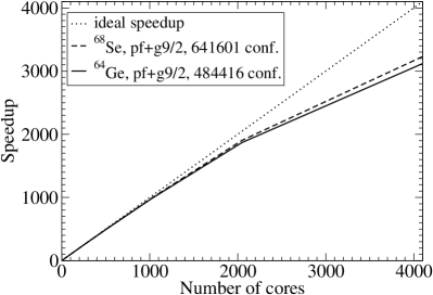
Figure 1: Speedup is defined as $T_{1}/T_{n}$, where $T_{n}$ is the calculation time, when $n$ processors were used. These calculations were performed on the FRANKLIN supercomputer at the National Energy Research Scientific Computing Center (NERSC) [35].

Hereafter we use the label $\alpha$ to denote a set of quantum numbers that includes either the fixed $M_{z}$ or the fixed $J$, keeping in mind that Eq. (11) can always connect them. In every important case we will point out which set of quantum numbers is used. Following the approach of [36], we can obtain the following expressions for the traces in Eqs. (9) and (10):

$$\mbox{Tr}^{(\alpha\kappa)}[H]=\sum_{i}\epsilon_{i}D^{[i]}_{\alpha\kappa}+\sum_{i<j}V_{ijij}D^{[ij]}_{\alpha\kappa},\;\;\;\;$$ (12)

$$\mbox{Tr}^{(\alpha\kappa)}[H^{2}]=\sum_{i}\epsilon^{2}_{i}D^{[i]}_{\alpha\kappa}+$$

$$+\sum_{i<j}\left[2\epsilon_{i}\epsilon_{j}+2(\epsilon_{i}+\epsilon_{j})V_{ijij}+\sum_{q<l}V^{2}_{ijql}\right]D^{[ij]}_{\alpha\kappa}+$$

$$+\sum_{(i<l)\neq l}\left[\sum_{q}\left(2V_{liiq}V_{ljjq}-V^{2}_{ijql}\right)+2\epsilon_{l}V_{ijij}\right]D^{[ijl]}_{\alpha\kappa}+$$

$$+\sum_{(i<j)\neq(q<l)}\left[V^{2}_{ijql}+V_{ijij}V_{qlql}-4V_{qiil}V_{qjjl}\right]D^{[ijql]}_{\alpha\kappa},\;\;\;\;$$ (13)

where $i,j,l,$ and $q$ are single-particle states with certain spin projections and possible occupation numbers equal 0 or 1.

Notice that the single-particle orbitals we have used to define the configurations in Eq. (1) can host all particles with all possible spin projections corresponding to spin of the orbital. The dimension factor $D^{[i]}_{\alpha\kappa}=\mbox{Tr}^{(\alpha\kappa)}[a^{\dagger}_{i}a_{i}]$ can be interpreted as a number of many-body states, possible for the configuration $\kappa$, with the fixed projection $M_{z}$ (if we consider $M_{z}$-traces) and under the condition that the single-particle state $i$ is occupied:

$$D^{[ij]}_{\alpha\kappa}=\mbox{Tr}^{(\alpha\kappa)}[a^{\dagger}_{i}a^{\dagger}_{j}a_{j}a_{i}],$$

$$D^{[ijq]}_{\alpha\kappa}=\mbox{Tr}^{(\alpha\kappa)}[a^{\dagger}_{i}a^{\dagger}_{j}a^{\dagger}_{q}a_{q}a_{j}a_{i}],...$$ (14)

These $D$-structures were called propagation functions in [36]. For completeness, we repeat here the recipe used for calculating them. One can show [36] that

$$D^{[r_{1}r_{2}\cdots r_{s}]}_{\alpha\kappa}=\sum_{s\leq t\leq n}(-1)^{t-s}\sum_{t_{1}+\cdots+t_{s}=t}D_{\alpha^{\prime}\kappa^{\prime}},$$ (15)

where all $t_{i}$ are non-negative integers, the configuration $\kappa^{\prime}=\{\kappa^{\prime}_{1},\kappa^{\prime}_{2},...\;,\kappa^{\prime}_{q}\}$ can be derived from the original configuration $\kappa=\{\kappa_{1},\kappa_{2},...\;,\kappa_{q}\}$ by removing $t$ particles from the single-particle states $r_{1},r_{2},\cdots r_{s}$. A formal expression for the new configuration $\kappa^{\prime}$ can be written as follows:

$$\kappa^{\prime}_{j}=\kappa_{j}-\sum_{i\;(r_{i}\in j)}t_{i},$$ (16)

where the sum includes only those values of $i$ for which the corresponding single-particle state $r_{i}$ belongs to the single-particle level $j$. We also assume that all the occupation numbers $\kappa^{\prime}_{j}$ must be positive, which imposes certain restrictions on the possible values of the amplitudes $t_{i}$. For every new configuration $\kappa^{\prime}$ one can easily define new quantum numbers, $\alpha^{\prime}=\{n^{\prime}M^{\prime}_{z}T^{\prime}_{z}\pi^{\prime}\}$, entering Eq. (15). Examples are the new number of particles $n^{\prime}=n-t$ and the new spin projection,

$$M^{\prime}_{z}=M_{z}-t_{1}m_{r_{1}}-t_{2}m_{r_{2}}-\cdots-t_{s}m_{r_{s}},$$ (17)

where $m_{r_{i}}$ is the $M_{z}$ projection of the single-particle state $r_{i}$. The new isospin $T^{\prime}_{z}$ and parity $\pi^{\prime}$ are defined similarly.

3 The algorithm for the method of moments in the proton-neutron formalism

Here we describe some technical features of the algorithm developed for the calculation of the nuclear level density. We treat protons and neutrons separately, so that the basis of many-body wave functions is represented by a product of proton and neutron parts:

$$|\nu,M_{z}\rangle=|\nu_{p},M^{(p)}_{z}\rangle\cdot|\nu_{n},M^{(n)}_{z}\rangle,$$ (18)

where $M^{(p)}_{z}+M^{(n)}_{z}=M_{z}$. The wave functions (18) have the fixed isospin projection $T_{z}$, but do not have a certain isospin $T$. As we already mentioned, it is more convenient to use the basis of the wave functions with the fixed spin projection $M_{z}$, rather than the one with the fixed spin $J$.

One could gain essential advantages from such a separation of the basis. One of them is related to the number of configurations that appear in the sum of Eq. (1). Naturally, the number of configurations with fixed $T_{z}$ is much greater than the number of configurations with fixed isospin. This allows the use of many-cores computers with greater efficiency. In other words, the calculation of the sum in Eq. (1) with a larger number of configurations can be more efficiently distributed over a larger number of processors. Fig. 1 presents the speedup (calculation speed gain) as a function of the number of used processors. One can see that the case with the larger number of configurations, ⁶⁸Se, scales better than the case with the lower number of configurations, ⁶⁴Ge. Up to 2000 cores, the speedup is almost perfect (the dotted line presents an ideal speedup). At this point the calculation time is about 1-2 minutes and further improvement is hardly achievable.

Another significant advantage of the proton-neutron formalism is the new algorithm of calculating the dimensions $D_{\alpha\kappa}$, $D^{[i]}_{\alpha\kappa}$, $D^{[ij]}_{\alpha\kappa}$, etc. Because of the proton-neutron separation one can calculate all proton and neutron dimensions separately. Later, the dimensions we are interested in can be easily constructed from the proton and neutron parts using the convolution,

$$D_{M_{z}\kappa}=\sum_{M^{(p)}_{z}+M^{(n)}_{z}=M_{z}}D_{M^{(p)}_{z}\kappa_{p}}\cdot D_{M^{(n)}_{z}\kappa_{n}},$$ (19)

where, instead of the whole set of quantum numbers $\alpha$, only the spin projection $M_{z}$ was explicitly indicated. Here $\kappa_{p}$ and $\kappa_{n}$ are the proton and neutron parts of the configuration $\kappa$. Eq. (19) can be easily applied to all types of dimensions, $D^{[\cdots]}_{\alpha\ldots}$, needed in the formalism of section II. The advantage comes from the fact that one can calculate and keep in memory all proton and neutron dimensions, $D_{M^{(p)}_{z}\kappa_{p}}$ and $D_{M^{(n)}_{z}\kappa_{n}}$, for all possible projections $M^{(p)}_{z}$ and $M^{(n)}_{z}$, and for all possible configurations $\kappa_{p}$ and $\kappa_{n}$. Afterwards, using Eqs. (19) and (15), one can calculate very fast all the dimensions: $D_{\alpha\kappa}$, $D^{[i]}_{\alpha\kappa}$, $D^{[ij]}_{\alpha\kappa}$, etc… , for all $M_{z}$ and $J$.

One more technical detail, which allows a significant speed up of the algorithm, is that by using the proton-neutron separation one can avoid multiple computations of the most time consuming structures, such as $D^{[ijql]}_{\alpha\kappa}$. Let us consider a case when all four single-particle states $\{ijql\}$ are protons. One can then use an equation similar to Eq. (19),

$$D^{[ijql]}_{M_{z}\kappa}=\sum_{M^{(p)}_{z}+M^{(n)}_{z}=M_{z}}D^{[ijql]}_{M^{(p)}_{z}\kappa_{p}}\cdot D_{M^{(n)}_{z}\kappa_{n}}.$$ (20)

For all configurations $\kappa$ that have the same proton parts $\kappa_{p}$ one would have to recalculate $D^{[ijql]}_{M^{(p)}_{z}\kappa_{p}}$ for each neutron configuration. Alternatively, one can calculate $D^{[ijql]}_{M^{(p)}_{z}\kappa_{p}}$ only once, and store the results in memory. That strategy, however, would require a large amount of storage. More efficiently, one can only store the contributions of the $D^{[ijql]}_{\alpha\kappa}$ structures to the width, Eq. (13), that is, one can only store the following $T$-structures,

$$T_{M^{(p)}_{z}\kappa_{p}}=\sum_{(i<j)\neq(q<l)}\left[V^{2}_{ijql}+V_{ijij}V_{qlql}\right.$$

$$\left.-4V_{qiil}V_{qjjl}\right]D^{[ijql]}_{M^{(p)}_{z}\kappa_{p}},$$ (21)

where all single-particle states are protons. Thus, instead of using Eq. (20) one can calculate the contribution to the width directly via the convolution,

$$\mbox{Tr}^{(\alpha\kappa)}[H^{2}]=\dots+\sum_{M^{(p)}_{z}+M^{(n)}_{z}=M_{z}}T_{M^{(p)}_{z}\kappa_{p}}\cdot D_{M^{(n)}_{z}\kappa_{n}},$$ (22)

which is very similar to Eqs. (19) and (20). The new approach avoids multiple calculations of $D^{[ijql]}_{M^{(p)}_{z}\kappa_{p}}$. Storing the structures Eq. (21), one may significantly speed up the algorithm for large cases, such as ⁶⁸Se in $pf+g_{9/2}$ model space. The downside is that the calculation of the $T$-structures, $T_{M^{(p)}_{z}\kappa_{p}},T_{M^{(n)}_{z}\kappa_{n}}$, does not always scale well on a large number of cores, since the number of these $T$-structures is much smaller than the total number of configurations.

4 Description of the program

The program consists of two separate codes. The first code is called MM, which is the main code in the program. MM code performs calculation of the first and second moments for all the configurations within the given range of spins and for certain parity. It is the most complicated and resource demanding part of the program. MM requires parallel computing. The second code is very simple and fast. It takes the output of the MM code (the first and second moments) and builds the nuclear level densities according to Eqs. (1-5). It does not require parallel computing.

Below we will concentrate only on description of the MM code. The detailed instructions on how to use the second code can be found in the readme.txt file, which is in the main project directory.

4.1 The structure of the MM code

In the MM code, the calculation of the first and second moments for a given nucleus is carried out. To compile this code simply follow the instructions in the readme.txt file (or type make) and then run the executable file mm.out.

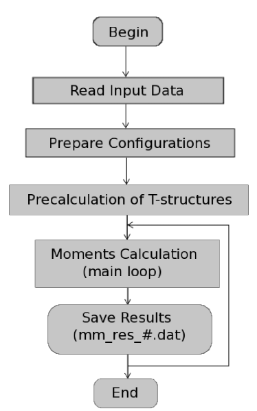
Figure 2: The flowchart of the program. See text for details.

The code contains four files: mm_1.15.f90 (1.15 is the current version) contains the main subroutines and calls subroutines from other files to perform the calculation; interaction.f90 reads the interaction file; angularme.for contains subroutines to work with the angular matrix elements, for example, to calculate Clebsch-Gordan coefficients; qsort.f contains quick-sort subroutines.

The flowchart of the mm_1.15.f90 is shown in Fig.2, and some important subroutines in the mm_1.15.f90 are listed below.

The subroutine prepare_interaction calculates the $T$-structures according to Eq. (21). This is an important part of the code which allows to speed up the program significantly.

The subroutine cc_density_calc contains the main loop over the configurations (the loop back in Fig. 2), calculates the first and second moments based on Eqs. (9,10,12,22), and saves the results. This subroutine uses the $T$-structures precalculated in the subroutine prepare_interaction.

Both subroutines require parallel computing. The simplest “Master-Slave” parallel programming paradigm with Dynamic Load Balancing was used.

4.2 MM input

The input files include input.dat and the files that define the single-particle model space as well as the interaction in this model space. A typical input.dat file that specifies the parameters in the code is listed below. The parameters are followed by their meaning:

6 6	! $Z\;N$
1 0 22 2	! $P\;2J_{{\rm min}}\;2J_{{\rm max}}\;2J_{{\rm step}}$
int/sd.spl	! single-particle model space
int/usd.int	! interaction

Here $Z$ and $N$ are the number of protons and neutrons, respectively, in the valence space; $P$ is parity ($P=1$ corresponds to positive parity and $P=-1$ to negative parity); $2J_{{\rm min}}$, $2J_{{\rm max}}$, and $2J_{{\rm step}}$ define the range of total spin for which the moments are to be calculated: the spin changes from the minimum value $J_{{\rm min}}$ to the maximum value $J_{{\rm max}}$ with the step $J_{{\rm step}}$. In the example listed above the total spin changes from 0 to 11 with the step 1. The single-particle model space and the interaction are defined by two separate files and input.dat must have the names of these two files similar to the shown example. Detailed description of *.spl and *.int files is given in the readme.txt file.

The above example describes the ²⁸Si nucleus in the $sd-$model space with the USD interaction. The moments will be calculated for positive parity and for all possible spins from 0 to 11.

4.3 MM output

The main output of the MM code is presented in files mm_res_#.dat. These files are enumerated by spin number #, for example mm_res_0.dat corresponds to spin $J=0$, mm_res_1.dat corresponds to spin $J=1/2$, and so on (for more details see the readme.txt file). Each output file contains the data needed for the density calculation: dimensions, first and second moments.

Another output file mm_conf.dat contains information about the configurations. This information is not used for the density calculation, but could be useful for checking and testing purposes.

4.4 Density calculation

After all the moments are prepared, the density can be calculated with the code den.out. The full description of density calculation can be found in the readme.txt file. We just repeat once more that there are several external parameters that need to be prepared before the calculation. These parameters cannot be defined within the method of moments, namely: $\eta$ - the cut-off parameter, $E_{{\rm g.s.}}$ - the ground state energy, and the energy interval $(E_{{\rm min}}$, $E_{{\rm max}})$ for calculating the level density. For more details see the readme.txt file.

5 Examples

Element	Space	Total dim	Elapsed time (sec)
70Br	$pf+g_{9/2}$	$10^{15}$	$1.07\cdot 10^{4}$
68Se	$pf+g_{9/2}$	$10^{15}$	$1.03\cdot 10^{4}$
64Ge	$pf+g_{9/2}$	$10^{14}$	$0.76\cdot 10^{4}$
60Zn	$pf$	$10^{11}$	37.4
52Fe	$pf$	$10^{10}$	13.6
28Si	$sd$	$10^{6}$	0.7

Table 1: Elapsed times of nuclear level density calculations (for all $J$, positive parity) with the moments method code. The calculations were done on a 16 cores machine with 2.8 GHz CPU frequency.

Table 1 presents calculation times for different nuclei calculated in different shell-model spaces. The calculations were done on a 16 cores machine with 2.8 GHz CPU frequency. One core (’master’) distributed all the work between other 15 cores (’slaves’). One can emphasize here that the listed times correspond to calculations of the nuclear level densities for all $J$ and for positive parity. For the case of ⁶⁸Se the largest $m$-scheme dimension is about $10^{15}$. For each $J$ the $m$-scheme dimensions vary from $10^{12}$ to $10^{14}$, which makes direct diagonalization impossible. Using the moments method and our algorithm we are able to calculate the shapes of nuclear densities for ⁶⁸Se in less then three hours on a 16 cores machine. For a number of processors reaching one thousand, it will take only few minutes to complete the calculation.

5.1 ²⁸Si, $sd-$model space

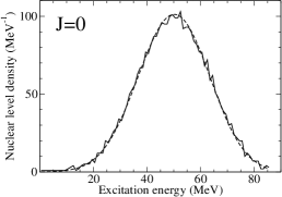
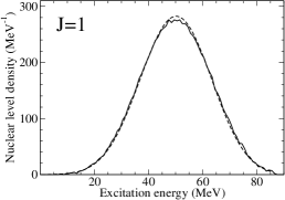
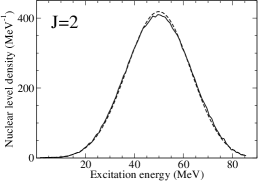
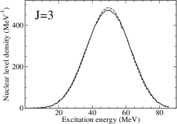
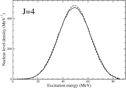
Figure 3: ²⁸Si, parity=+1. Comparison of nuclear level densities between the exact shell model (solid line) and the moments method (dashed line). Cut-off parameter $\eta=2.8$, interaction: USD, $sd$-shell.

As a first example we consider the level density for the ²⁸Si nucleus in the $sd$-shell model space, where we use the USD interaction [37]. Fig. 3 presents the comparison of the exact shell-model level densities for different spins (solid lines) with those obtained with the moments methods (dashed lines).

Eqs. (1) and (2) require the knowledge of the ground state energy $E_{{\rm g.s.}}$ and the cut-off parameter $\eta$. While the ground state energy of ²⁸Si can be calculated in this case using the standard shell model, $E_{{\rm g.s.}}=-135.94$ MeV, for the value of the cut-off parameter $\eta$ we have only a general idea that it should be around 3 [22, 23]. For a better description of level densities in the moments method we can adjust the $\eta$ parameter to optimally reproduce the exact shell-model densities. From Fig. 3 one can see that choosing $\eta=2.8$, the level densities of the moments method reproduce quite well the exact shell-model level densities. The cut-off parameter plays a role similar to that of the width in a Gaussian distribution. Indeed, if we increase the cut-off parameter, the density becomes wider and lower, while decreasing it leads to a narrowing of the density. One should also mention that the exact spin- and parity-dependent shell-model densities were calculated with the NuShellX code [38].

5.2 ⁶⁴Ge, $pf-$ and $pf+g9/2-$model spaces

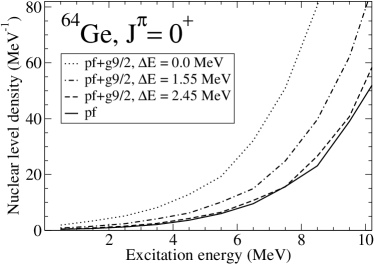
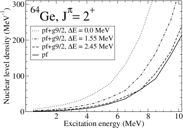
Figure 4: Level densities for the ⁶⁴Ge nucleus, $J=0,2$ and positive parity. Solid line presents the calculation in the $pf$-shell with the GXPF1A interaction. For this calculation we know the ground state energy, $E_{{\rm g.s.}}(pf)=-304.25$ MeV. Other three lines present calculations in the large model space, when level $g_{9/2}$ is added. The ground state energy for these cases is $E_{{\rm g.s.}}(pf+g_{9/2})=E_{gs}(pf)-\Delta E$, where $\Delta E$ is the energy shift. The cut-off parameter is $\eta=2.6$.

As mentioned in the Introduction, one could envision using information from the level densities to extract with a good approximation the ground state energies. Using our algorithm and the moments method one can easily calculate the nuclear level density for any nucleus that can be described in the $pf+g_{9/2}$ model space. The Hamiltonian used for this model space was built starting with the GXPF1A interaction for the $pf$ model space, to which the $G$-matrix elements that describe the interaction between the $pf$ orbits and $g_{9/2}$ orbit were added. The single-particle energy for the $g_{9/2}$ orbit was fixed at $-$0.637 MeV. Even for the worst case, the calculation takes about three hours for sixteen processors and only few minutes for one thousand processors. Fig. 4 presents the results obtained for ⁶⁴Ge, nucleus that is believed to be a “waiting-point” along the $rp$-process path [39-41]. We only present the densities for $J=0,2$ and positive parity.

The corresponding input.dat file for ⁶⁴Ge in $pf-$model space looks like

12 12	! $Z\;N$
1 0 22 2	! $P\;2J_{{\rm min}}\;2J_{{\rm max}}\;2J_{{\rm step}}$
int/pf.spl	! single-particle model space
int/gx1a.int	! interaction

Here we have twelve protons and twelve neutrons in the $pf$-model space. The calculation is done for all spins between $J=0$ and $J=11$ and positive parity. The single-particle space is defined in the pf.spl file and the interaction is in gx1a.int. For the $pf+g9/2$ model space we need to change the single-particle file to pfg9.spl and the interaction file to pfg9.int.

It is important to notice that in the $pf$ model space the shell-model calculations of the ground state energies can be done. For ⁶⁴Ge in the $pf$-shell we obtain the following ground state energy:

$$E_{{\rm g.s.}}(pf)=-304.25\mbox{ MeV.}$$ (23)

Using this ground state energy and the cut-off parameter $\eta=2.6$, we are able to calculate the level densities according to Eqs. (1) and (2). The solid lines in Fig. 4 represent the density in the $pf$-shell.

To calculate the same level density in the $pf+g_{9/2}$ model space we have to adjust the ground state energy and the cut-off parameter for this space. For the cut-off parameter we use the same value, $\eta=2.6$, but it is practically impossible to calculate by shell-model diagonalization the ground state energy since the dimension is too large. The ground state energy for the larger model space, that is $pf+g_{9/2}$, must be lower compared to the ground state energy for the smaller model space, that is $pf$. Let us introduce this energy difference, $\Delta E$, as

$$E_{{\rm g.s.}}(pf+q_{9/2})=E_{{\rm g.s.}}(pf)-\Delta E.$$ (24)

The dotted lines in Fig. 4 show the level densities if we keep the ground state energy for $pf+g_{9/2}$ model space as it was in the $pf$ case keeping $\Delta E=0$. It is natural to expect only small differences between the level densities calculated in those two model spaces at low excitation energy since in the $pf+g_{9/2}$ model space we use the same GXPF1A interaction for the $pf$ subspace. By decreasing the ground state energies for the $pf+g_{9/2}$ model space (introducing non-zero $\Delta E$), one gets the dashed lines on Fig. 4. The dash-dotted lines there correspond to ground state energy $E_{{\rm g.s.}}(pf+q_{9/2})=-305.8$ MeV of ⁶⁴Ge, which was obtained by a truncated shell model calculation with up to 6 particles excited from the $f_{7/2}$ orbits and/or into the $g_{9/2}$ orbit. The $m$-scheme dimension in this calculation, $13.5\times 10^{9}$, is at the upper limit of the state of the art shell-model calculation. As one can see, this value does not describe satisfactory the level densities at low excitation energy. In order to make the low-lying part of the two densities very close (dashed and solid lines on Fig. 4), one has to adjust the ground state energy for the $pf+g_{9/2}$ model space to the following value:

$$E_{{\rm g.s.}}(pf+g_{9/2})=-306.7\;\mbox{ MeV for }\;{}^{64}\;\mbox{Ge},\\$$ (25)

The “low-lying part of the density” should be chosen such that the excitations to the $g_{9/2}$ orbit do not give a significant contribution. For these cases we use the interval 3-6 MeV in excitation energy. We conclude that the adjustment of Eq. (25) can be treated as a method for estimating the ground state energies in larger spaces; for more details see [25].

6 Summary

In summary, we have developed an efficient Fortran code for calculating the centroids and widths of the shell-model spin- and parity-dependent configurations, which can be used for calculating the nuclear level densities. The code is parallelized using the Message Passing Interface (MPI) [34] and a master-slaves dynamical load-balancing approach. The parallel code was thoroughly tested on the massively parallel computers at NERSC [35], and it shows very good scaling when using up to 4000 cores. The algorithm used takes advantage of the separation of the model space in neutron and proton subspaces. This separation provides two important advantages: (i) the exponentially exploding dimensions and propagators can be calculated more efficiently in proton and neutron subspaces, and the full results can be recovered via simple convolutions; (ii) the number of configurations is significantly increased in the proton-neutron formalism, considerably improving the scalability of the algorithm on massively parallel computers. Our tests indicate almost perfect scaling for up to 4000 cores. The new algorithm is so fast that the bottleneck of the calculation is now that of the ground state energy. That is why we could not test our algorithm for cases that take more than one minute on 4000 cores. Therefore, we investigated the possibility of using the calculated shapes of the nuclear level densities to extract the ground state energy. We showed that by incrementing the model space and the effective interaction, and imposing the condition that the level density does not change at low expectation energy, one can reliably predict the ground state energy, and further the full level density. This new method of extracting the shell model ground state energy for model spaces whose dimensions are unmanageable for direct diagonalization opens new opportunities for calculating shell model level densities of heavier nuclei of interest for nuclear astrophysics, nuclear energy and medical physics applications.

A further development of the application of statistical spectroscopy to nuclear level density is the removal of center-of-mass spurious states from the level density for shell model spaces that allow complete factorization of the center-of-mass and intrinsic wave functions. A new algorithm implementing this idea was recently presented [42], and a high performance code was developed. This new code could be made available upon request.

7 Acknowledgments

R.A.S. and M.H. would like to acknowledge the DOE UNEDF grant DE-FC02-09ER41584 for support. M.H. and V.Z. acknowledge support from the NSF grant PHY-1068217.

References

- [1] W. Hauser and H. Feshbach, Phys. Rev. 87 (1952) 366.
- [2] T. Rauscher, F.-K. Thielemann, and K.-L. Kratz, Phys. Rev. C 56 (1997) 1613.
- [3] P. Möller et. al., Phys. Rev. C 79 (2009) 064304.
- [4] H. A. Bethe, Phys. Rev. 50 (1936) 332.
-
[5]
A.G.W. Cameron, Can. J. Phys. 36 (1958) 1040;
A. Gilbert and A.G.W. Cameron, Can. J. Phys. 43 (1965) 1446-1496. - [6] T. Ericson, Nucl. Phys. 8, 265 (1958); Adv. Phys. 9 (1960) 425.
- [7] S. Goriely, S. Hilaire, and A. J. Koning, Phys. Rev. C 78 (2008) 064307.
- [8] S. Goriely, S. Hilaire, A. J. Koning, M. Sin, and R. Capote, Phys. Rev. C 79 (2009) 024612.
- [9] H. Uhrenholt, S. Åberg, P. Möller, and T. Ichikawa, arXiv:0901.1087.
- [10] W. E. Ormand, Phys. Rev. C 56 (1997) R1678.
- [11] H. Nakada and Y. Alhassid, Phys. Rev. Lett. 79 (1997) 2939.
- [12] K. Langanke, Phys. Lett. B 438 (1998) 235.
- [13] Y. Alhassid, G. F. Bertsch, S. Liu, and H. Nakada, Phys. Rev. Lett. 84 (2000) 4313.
- [14] Y. Alhassid, S. Liu, and H. Nakada, Phys. Rev. Lett. 99 (2007) 162504.
- [15] Y. Alhassid, L. Fang, and H. Nakada, Phys. Rev. Lett. 101 (2008) 082501.
- [16] E. Teran and C.W. Johnson, Phys. Rev. C 73 (2006) 024303.
- [17] E. Teran and C.W. Johnson, Phys. Rev. C 74 (2006) 067302.
- [18] http://www-astro.ulb.ac.be/Html/nld.html
- [19] T. von Egidy and D. Bucurescu, Phys. Rev C 80 (2009) 054310.
- [20] M. Horoi, M. Ghita, and V. Zelevinsky, Nucl. Phys. A785 (2005) 142c.
- [21] D. Mocelj, T. Rauscher, G. Martinez-Pinedo, K. Langanke, L. Pacearescu, A. Faessler, F.-K. Thielemann, and Y. Alhassid, Phys. Rev. C 75 (2007) 045805.
- [22] M. Horoi, J. Kaiser, and V. Zelevinsky, Phys. Rev. C 67 (2003) 054309.
- [23] M. Horoi, M. Ghita, and V. Zelevinsky, Phys. Rev. C 69 (2004) 041307(R).
- [24] M. Horoi and V. Zelevinsky, Phys. Rev. Lett. 98 (2007) 262503.
- [25] R.A. Sen’kov and M. Horoi, Phys. Rev. C 82 (2010) 024304.
- [26] M. Hjorth-Jensen, T.S. Kuo and E. Osnes, Phys. Rep. 261 (1995) 125.
- [27] J.B. French and V.K.B. Kota, Phys. Rev. Lett. 51 (1983) 2183.
- [28] S. S. M. Wong, Nuclear Statistical Spectroscopy (Oxford University Press, 1986).
- [29] M. Horoi, A. Volya, and V. Zelevinsky, Phys. Rev. Lett. 82 (1999) 2064.
- [30] M. Horoi, B.A. Brown, and V. Zelevinsky, Phys. Rev. C 65 (2002) 027303.
- [31] M. Horoi, B.A. Brown, and V. Zelevinsky, Phys. Rev. C 67 (2003) 034303.
- [32] Z.C. Gao and M. Horoi, Phys. Rev. C 79 (2009) 014311.
- [33] Z.C. Gao, M. Horoi, and Y.S. Chen, Phys. Rev. C 80 (2009) 034325.
- [34] www.mcs.anl.gov/mpi .
- [35] www.nersc.gov .
-
[36]
C. Jacquemin and S. Spitz, J. Phys. G 5 (1979) 195;
C. Jacquemin, Z. Phys. A 303 (1981) 135. - [37] B. A. Brown and B. H. Wildenthal, Annu. Rev. Nucl. Part. Sci. 38 (1988) 29.
- [38] W. Rae, NuShellX (2008), http://knollhouse.org/NuShellX.aspx.
- [39] H. Schatz, at al., Phys. Rep. 294 (1998) 167.
- [40] J. A. Clark et al., Phys. Rev. C 75 (2007) 032801(R).
- [41] P. Schury et al., Phys. Rev. C 75 (2007) 055801.
- [42] R.A. Senkov, M. Horoi, and V. Zelevinsky, Phys. Lett. B 702 (2011) 413.