SIMILARITIES IN POPULATIONS OF STAR CLUSTERS

Abstract

We compare the observed mass functions and age distributions of star clusters in six well-studied galaxies: the Milky Way, Magellanic Clouds, M83, M51, and Antennae. In combination, these distributions span wide ranges of mass and age: $10^{2}{\>\hbox to0.0pt{\raise 2.0pt\hbox{$<$}\hss}\lower 3.0pt\hbox{$\sim$}\>}M/M_{\odot}{\>\hbox to0.0pt{\raise 2.0pt\hbox{$<$}\hss}\lower 3.0pt\hbox{$\sim$}\>}10^{6}$ and $10^{6}{\>\hbox to0.0pt{\raise 2.0pt\hbox{$<$}\hss}\lower 3.0pt\hbox{$\sim$}\>}\tau/\mbox{yr}{\>\hbox to0.0pt{\raise 2.0pt\hbox{$<$}\hss}\lower 3.0pt\hbox{$\sim$}\>}10^{9}$. We confirm that the distributions are well represented by power laws: $dN/dM\propto M^{\beta}$ with $\beta\approx-1.9$ and $dN/d\tau\propto\tau^{\gamma}$ with $\gamma\approx-0.8$. The mass and age distributions are approximately independent of each other, ruling out simple models of mass-dependent disruption. As expected, there are minor differences among the exponents, at a level close to the true uncertainties, $\epsilon_{\beta}\sim\epsilon_{\gamma}\sim$ 0.1–0.2. However, the overwhelming impression is the similarity of the mass functions and age distributions of clusters in these different galaxies, including giant and dwarf, quiescent and interacting galaxies. This is an important empirical result, justifying terms such as “universal” or “quasi-universal.” We provide a partial theoretical explanation for these observations in terms of physical processes operating during the formation and disruption of the clusters, including star formation and feedback, subsequent stellar mass loss, and tidal interactions with passing molecular clouds. A full explanation will require additional information about the molecular clumps and star clusters in galaxies beyond the Milky Way.

1 INTRODUCTION

Star clusters form in the dense parts (“clumps”) of molecular clouds (Lada & Lada 2003; McKee & Ostriker 2007). They are subsequently destroyed by several processes, beginning with the expulsion of residual gas by massive young stars (“feedback”), further mass loss from intermediate- and low-mass stars, tidal disturbances by passing molecular clouds, and stellar escape driven by internal two-body relaxation (Binney & Tremaine 2008). These processes disperse the stars from clusters into the surrounding stellar field. Star clusters therefore represent an intermediate stage in the transformation of the clumpy interstellar medium (ISM) of a galaxy into a relatively smooth stellar distribution.

In this paper, we show that there are some remarkable similarities in the statistical properties of cluster populations in different galaxies. In particular, we focus on the univariate mass and age distributions, $\psi(M)\propto dN/dM$ and $\chi(\tau)\propto dN/d\tau$, and the bivariate mass–age distribution, $g(M,\tau)\propto\partial^{2}N/\partial{M}\partial{\tau}$. These distributions encode valuable information about the formation and disruption of clusters, for example, whether less massive ones dissolve faster than more massive ones. In the next section, we present the mass and age distributions of the clusters in six well-studied galaxies, based on published data, but now displayed in a uniform manner. In the following section, we provide a partial theoretical explanation for these observations, and in the last section, we summarize and place our results in the context of other work in this field.

As in our previous papers, we use the term “cluster” for any concentrated aggregate of stars with a density much higher than that of the surrounding stellar field, whether or not it also contains gas, and whether or not it is gravitationally bound. This is the standard definition in the star formation community (Lada & Lada 2003; McKee & Ostriker 2007). Some authors use the term “cluster” only for gas-free or gravitationally bound objects. We reject these definitions for several reasons. (1) They ignore the fact that gas-free and gas-rich clusters (including molecular clumps and HII regions) are the same objects observed in different evolutionary phases. (2) It is impossible to tell from images alone which clusters are gravitationally bound (have negative energy) and which are unbound (have positive energy). In principle, spectra would help, but in practice, they are seldom available and are often contaminated by non-virial motions (stellar winds, binary stars, etc). (3) $N$-body simulations show that unbound clusters retain the appearance of bound clusters for many ($\sim$10–50) crossing times (Baumgardt & Kroupa 2007). By “disruption,” we mean the removal of mass from a cluster, whether this occurs gradually or suddenly, and whether it leaves the cluster bound or unbound.

2 MASS AND AGE DISTRIBUTIONS

Figures 1 and 2 show the mass functions and age distributions of the clusters in six nearby galaxies. The mass functions are plotted for several disjoint age intervals and the age distributions for several disjoint mass intervals. These figures are based on data from Lada & Lada (2003) for the solar neighborhood in the Milky Way, Chandar et al. (2010a) for the Large and Small Magellanic Clouds (LMC and SMC), Chandar et al. (2010c) for a large field in M83, Chandar et al. (2011) for M51, and Fall et al. (2009) for the Antennae. For the clusters in the solar neighborhood, the masses and ages were derived from photometry of individual stars; for the clusters in the other galaxies, they were derived from integrated photometry in several wavebands (usually $UBVI{\rm H}\alpha$) and comparisons with stellar population models. The H$\alpha$ photometry is crucial for distinguishing clusters younger and older than $\sim$$10^{7}$ yr. Lada & Lada (2003) and Chandar et al. (2010b) describe these methods in more detail.

For ease of comparison, we have made two simple adjustments to the published mass and age distributions when constructing Figures 1 and 2. First, we replotted them in a uniform format: $\log(dN/dM)$ against $\log(M/M_{\odot})$ and $\log(dN/d\tau)$ against $\log(\tau/{\rm yr})$. For the solar neighborhood, the original distributions were presented in the form $\log(MdN/d\log{M})$ against $\log(M/M_{\odot})$ and $\log(dN/d\log{\tau})$ against $\log(\tau/{\rm yr})$. Second, we adopted a uniform conversion from light to mass based on stellar population models with the Chabrier (2003) IMF. For the LMC, SMC, M51, and Antennae, the original distributions were based on models with the Salpeter (1955) IMF, which have $\Delta\log{M}=0.2$ and $\Delta\log{\tau}=0.0$ relative to models with the Chabrier (2003) IMF.

The observed mass and age distributions are well represented by featureless power laws:

$$dN/dM\propto M^{\beta},$$ (1)

$$dN/d\tau\propto\tau^{\gamma}.$$ (2)

We list the best-fit exponents and their formal $1\sigma$ errors for the 12 mass functions and 10 age distributions in Tables 1 and 2. The straight lines in Figures 1 and 2 show the corresponding power laws. Both the mean and median exponents for this sample are $\beta=-1.9$ and $\gamma=-0.8$, and the standard deviations of individual exponents about the means are $\sigma_{\beta}=0.15$ and $\sigma_{\gamma}=0.18$ (with full ranges $-2.24\leq\beta\leq-1.70$ and $-1.05\leq\gamma\leq-0.54$). As a result of stochastic fluctuations in the luminosities and colors of clusters, the true uncertainties (errors) in the exponents, $\epsilon_{\beta}$ and $\epsilon_{\gamma}$, are usually larger than the formal $1\sigma$ errors listed in Tables 1 and 2, with typical values $\epsilon_{\beta}\sim\epsilon_{\gamma}\sim$ 0.1–0.2 (Fouesneau et al. 2012). Since these are similar to the dispersions $\sigma_{\beta}$ and $\sigma_{\gamma}$, we cannot tell whether the small differences among the exponents are real, although we do expect differences at roughly this level, as explained below.

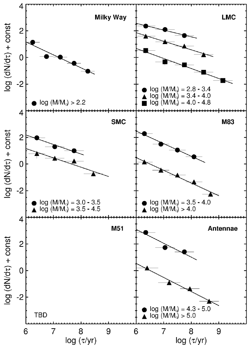
Figure 2: Age distributions of star clusters in different mass intervals in different galaxies (as indicated). These have been adapted from the references given in the text. The absolute normalizations of the age distributions are arbitrary, but the relative normalizations within each panel are preserved. The vertical spacing between the age distributions depends on the adopted mass intervals, which differ among the galaxies for practical reasons (distance, limiting magnitude, sample size). The lines show power laws, $dN/d\tau\propto\tau^{\gamma}$, with the best-fit exponents listed in Table 2. Note that these are all close to $\gamma=-0.8$.

Figures 1 and 2 show that the mass and age distributions are essentially independent of each other. This follows from the parallelism of the mass functions in different age intervals and the age distributions in different mass intervals. The vertical spacing between the age distributions differs only because the adopted mass intervals differ, a consequence of the different distances, limiting magnitudes, and sample sizes among the galaxies. Thus, we can approximate the bivariate mass–age distribution as a product of the two univariate distributions:

$$g(M,\tau)\propto\psi(M)\chi(\tau)\propto M^{\beta}\tau^{\gamma}.$$ (3)

We originally introduced this model for clusters in the Antennae, with the speculation that it might also apply to clusters in other galaxies (Fall et al. 2005; Fall 2006; Whitmore et al. 2007). We emphasize that, for each galaxy, our power-law fits are based on data in large, but limited, ranges of mass and age, typically $\Delta\log{M}\sim\Delta\log{\tau}\sim 2$. In combination, however, they span even wider ranges, roughly $10^{2}\lesssim M/M_{\odot}\lesssim 10^{6}$ and $10^{6}\lesssim\tau/{\rm yr}\lesssim 10^{9}$.

The age distribution, in general, reflects the difference between the formation and disruption rates of clusters. We know from observations that the star formation rate has remained roughly constant, within factors of 2–3, during the past $10^{9}$ yr in the solar neighborhood (Wyse 2009 and references therein), LMC (Harris & Zaritsky 2009), and SMC (Harris & Zaritsky 2004). Simulations indicate that this rate has also varied slowly in the Antennae for at least the past $10^{8}$ yr and possibly $10^{9}$ yr (Karl et al. 2011). The formation rates of stars and clusters likely track each other closely, simply because most stars form in clusters (Lada & Lada 2003; McKee & Ostriker 2007). A factor of 2–3 variation in the formation rate of clusters between $\tau\sim 10^{6}$ yr and $10^{9}$ yr would change the exponent of the age distribution by only $\Delta\gamma\approx$ 0.10–0.17. This is similar to the dispersion among galaxies and the true uncertainty mentioned above ($\sigma_{\gamma}\sim\epsilon_{\gamma}\sim$ 0.1–0.2) and is much smaller than the magnitude of the typical exponent, $|\gamma|\approx 0.8$. Thus, we are confident that most of the observed decline in the age distributions is caused by the disruption of clusters rather than variations in their formation rate.

Two important conclusions now follow directly from Figures 1 and 2 and Equations (1)–(3). First, the shape of the mass function $\psi(M)$ is preserved over wide ranges of age, although its amplitude, proportional to the age distribution $\chi(\tau)$, declines by a large factor. Thus, there is no evidence for mass-dependent disruption of clusters in this sample of well-studied galaxies. Second, both the mass and age distributions are remarkably similar from one galaxy to another, with differences mostly attributable to observational uncertainties. Thus, there is little if any evidence for galaxy-dependent disruption of clusters in this sample, which includes giant and dwarf, quiescent and interacting galaxies. This degree of similarity in an astronomical setting probably justifies the adjective “universal.” However, since we expect and possibly observe minor differences among the mass and age distributions in different galaxies, we sometimes employ the more modest term “quasi-universal.”

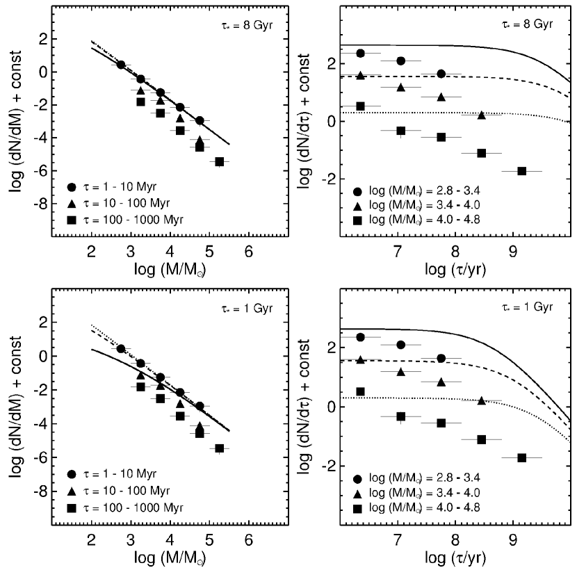
Figure 3: Mass functions and age distributions of star clusters in the LMC (left-hand and right-hand panels, respectively). The data points are the same as in Figures 1 and 2. The curves are based on a simple model with gradual mass-dependent disruption, computed from Equation (12) of Fall et al. (2009) with $\beta=-2$, $k=0.6$, and either $\tau_{*}=8$ Gyr (top panels) or $\tau_{*}=1$ Gyr (bottom panels). The three curves in each panel correspond to the same age and mass intervals as the data points. Note that the models are poor fits to all the data, except the mass function at the youngest ages ($\tau\leq 10^{7}$ yr).

It is also worth asking what the mass and age distributions would look like if the disruption were mass dependent. Figure 3 helps to answer this question. The curves in this diagram are based on a model in which clusters form at a constant rate with a power-law initial mass function and are then disrupted gradually at the following mass-dependent rate:

$$dM/d\tau=-M/\tau_{d}(M),$$ (4)

$$\tau_{d}(M)=\tau_{*}(M/10^{4}M_{\odot})^{k}.$$ (5)

Boutloukos & Lamers (2003) claim that this model represents an “empirical disruption law,” in which different galaxies have nearly the same exponents, $k\approx 0.6$, but timescales $\tau_{*}$ that differ by more than two orders of magnitude. It is therefore both mass dependent and galaxy dependent. Fall et al. (2009) derived analytical formulae for the mass and age distributions for this and other disruption models. For the LMC clusters, de Grijs & Anders (2006) advocate the parameter values $k=0.6$ and $\tau_{*}=8\times 10^{9}$ yr. As Figure 3 shows, this model fails by a wide margin to match the observed mass and age distributions of the LMC clusters. Chandar et al. (2010a, 2010c, 2011) present similar comparisons and failures for the SMC, M83, and M51 clusters.

A key point illustrated by Figure 3 is that any mass dependence in the disruption rate will introduce features in both the mass and age distributions. These occur at $M_{d}(\tau)=10^{4}(\tau/\tau_{*})^{1/k}M_{\odot}$ and $\tau_{d}(M)=\tau_{*}(M/10^{4}M_{\odot})^{k}$, respectively. For $M\gtrsim M_{d}(\tau)$ and $\tau\lesssim\tau_{d}(M)$, the mass function retains its initial shape and amplitude, while the age distribution remains flat. Conversely, for $M\lesssim M_{d}(\tau)$ and $\tau\gtrsim\tau_{d}(M)$, the mass function becomes shallower, while the age distribution steepens. We note that these signatures of mass-dependent disruption are even more prominent in the age distribution than in the mass function and would be easy to detect if they were present. As we have already emphasized, there are no such features in the observed distributions displayed in Figures 1 and 2.

The mass and age distributions compiled here are based on samples of clusters that are complete or unbiased with regard to mass and age. We caution readers that some of the distributions in the literature are based on samples with less suitable selection criteria. The completeness of the samples may be poorly known and/or vary with mass and age; clusters may be excluded if they are located in crowded regions, have uncertain photometry, or are somehow deemed to be unbound. Selection biases such as these can easily cause deviations from power laws in the mass and age distributions, as demonstrated explicitly by Fall et al. (2009) and Chandar et al. (2010a). Stochastic fluctuations in the luminosities and colors of clusters are another cause of spurious features in these distributions, especially when relatively narrow mass and age bins are chosen (e.g., the RSG “gap” at $\tau\approx$ (1–3) $\times 10^{7}$ yr; Fall et al. 2005; Fouesneau et al. 2012).

Some authors also claim to find an exponential steepening of the mass function for $M\gtrsim M_{c}\sim 10^{5}M_{\odot}$ (Larsen 2009). These claims, however, are based on the absence of only a few clusters relative to extrapolated power laws and thus have little statistical significance (Chandar et al. 2010b). The mass functions displayed in Figure 1 do not even hint at such steepening. If they did, it would be appropriate to replace the power law in Equation (3) by a Schechter function, giving $g(M,\tau)\propto M^{\beta}\tau^{\gamma}\exp(-M/M_{c})$. We note that this mass–age distribution also represents mass-independent disruption (for $M_{c}={\rm const}$) because it is still of separable form, $g(M,\tau)\propto\psi(M)\chi(\tau)$. This illustrates an important point: features in the mass function are not by themselves evidence for mass-dependent disruption.

Bastian et al. (2012) have presented new mass and age distributions for clusters in two fields in M83, including the one studied by Chandar et al. (2010c). We have checked that these distributions are mostly consistent with those derived by Chandar et al. and reproduced here in Figures 1 and 2. The discrepancies are relatively small and can be attributed to selection biases of the type mentioned above. The Bastian et al. samples are incomplete for young clusters of all masses ($\tau\lesssim 10^{7}$ yr), for older low-mass clusters ($\tau\gtrsim 10^{8}$ yr and $M\lesssim 10^{4}M_{\odot}$), and for clusters in crowded regions. When we apply these selection biases to the more complete Chandar et al. sample, we introduce artificial features in the mass and age distributions, mimicking those in the Bastian et al. distributions. We are currently analyzing complete samples of clusters in these and several more fields in M83 and will present the results in a separate paper.

3 FORMATION AND DISRUPTION PROCESSES

In this section, we discuss the physical processes most likely to have shaped the observed mass and age distributions shown in Figures 1 and 2. Before proceeding, we emphasize that our power-law models for $\psi(M)$, $\chi(\tau)$, and $g(M,\tau)$ are convenient fitting formulae suggested directly by observations and, as such, are valid irrespective of any theoretical interpretation. It is also worth emphasizing that we currently lack some auxiliary information needed to construct a definitive explanation for the mass and age distributions. There are, for example, no surveys of molecular clumps in galaxies beyond the Milky Way. We also lack accurate measurements of the internal structure of large and complete samples of extragalactic star clusters. Nevertheless, we have enough theoretical and observational knowledge to construct a partial explanation of the mass and age distributions as follows.

The observed mass functions of molecular clouds and clumps in the Milky Way are power laws with exponents $\beta\approx-1.7$ (Shirley et al. 2003; Rosolowsky 2005; Muñoz et al. 2007; Wong et al. 2008). Because more massive clouds and clumps have longer lifetimes than less massive ones, they are overrepresented in the samples from which the mass functions are derived. Thus, the initial mass function, corrected for this effect, must be slightly steeper than the observed one. The result of this correction is $\beta\approx-2.0$ for clouds and clumps, nearly identical to the exponent for clusters (Fall et al. 2010). This is what we would expect to find if all the gas in the clumps (protoclusters) were converted into stars, i.e., if the efficiency of star formation ${\cal E}$ were 100%. In fact, however, the efficiency is much lower: ${\cal E}\approx$ 20%–30% in the dense clumps where clusters form and a factor of $\sim$10 lower still in the larger and more diffuse clouds that contain the clumps (Lada & Lada 2003). Thus, to explain why the mass function of clusters is a power law with exponent $\beta\approx-1.9$, we must explain why the efficiency of star formation ${\cal E}$ is independent (or nearly so) of the masses of their antecedent clumps.

Stars form in a protocluster until their output of energy and momentum has expelled the remaining gas. This stellar feedback potentially includes radiation pressure on dust grains, photoionized gas pressure, protostellar outflows, main-sequence winds, and supernovae. It is likely that radiation pressure predominates in massive protoclusters and that supernovae, because they come after the other feedback processes, are relatively ineffective at removing gas (Krumholz & Matzner 2009; Murray et al. 2010). The condition that feedback can accelerate the remaining gas to the escape speed then leads to formulae for ${\cal E}(M)$ (Fall et al. 2010). These depend on whether the feedback is closer to the energy-driven limit (with negligible radiative losses) or to the momentum-driven limit (with maximum losses) and the relation between the escape speed and the masses of the clumps or, equivalently, their characteristic radius–mass relation, which we approximate by a power law, $R\propto M^{\alpha}$. Most of the feedback in the dense protoclusters is momentum driven (see Table 1 of Fall et al. 2010), and in this limit, we have ${\cal E}\propto M^{1-2\alpha}$.

Fall et al. (2010) showed that there is a strong correlation between the radii and masses of molecular clumps, with $\alpha\approx 0.4$, based on measurements of CS, C¹⁷O, and 1.2 mm dust emission in the independent surveys by Shirley et al. (2003), Faúndez et al. (2004), and Fontani et al. (2005). The more recent survey by Wu et al. (2010), based on measurements of different molecular tracers, confirms this correlation, with $\alpha\approx 0.5$ (see their Figures 31–34). These radius–mass relations imply ${\cal E}(M)\approx{\rm constant}$ for momentum-driven feedback. Thus, we have a simple physical explanation for the similarity between the mass functions of clumps and clusters. It remains, then, to explain the power-law form of the mass function of the clumps in terms of physical processes in the turbulent ISM, an important challenge beyond the scope of this paper.

Following the expulsion of natal gas from a cluster, it will continue to lose mass from its member stars during the normal course of stellar evolution (through winds and other ejecta). Stellar mass loss itself removes only 10%–50% of the mass of a cluster (depending on its age, metallicity, and stellar IMF), but if the cluster is weakly bound and resides in a tidal field, it can be partially or even completely disrupted by this process (Chernoff & Weinberg 1990). This happens because the cluster cannot maintain a state of virial equilibrium (Fukushige & Heggie 1995). Clusters with low concentrations, $c\equiv\log(r_{t}/r_{c})\lesssim 0.7$ (where $r_{t}$ and $r_{c}$ are the tidal and core radii), are particularly vulnerable. In terms of the dimensionless central potential, this condition is equivalent to $W_{0}\lesssim 0.3$. We expect such weakly bound clusters to be numerous as a result of the earlier expulsion of gas by stellar feedback.

The effect of this disruption process on the mass and age distributions of the clusters depends primarily on their concentrations—for clusters with the same stellar IMF, until two-body evaporation becomes important (Chernoff & Weinberg 1990; Fukushige & Heggie 1995). In particular, the shape of the mass function will be preserved, while its amplitude declines, so long as $c$ is not correlated with $M$. This is a reasonable expectation because the star formation efficiency ${\cal E}$, which determines the relative weakening of the gravitational potential of the clusters by stellar feedback, is independent of $M$. The top panel of Figure 4 shows $c$ plotted against $M$ for LMC and SMC clusters from fits of King profiles to Hubble Space Telescope (HST) images by McLaughlin & van der Marel (2005). Evidently, there is no correlation between $c$ and $M$, consistent with the fact that the mass function has the same power-law shape at all ages. This result is suggestive rather than definitive, however, because it involves only a small fraction of clusters in the LMC and SMC.

Star clusters can also be disrupted by tidal interactions with passing molecular clouds. Spitzer (1958) proposed this mechanism to account for the scarcity of clusters older than $\sim$$10^{9}$ yr in the galactic disk. We follow the comprehensive treatment by Binney & Tremaine (2008) and distinguish two regimes: catastrophic, in which clusters are disrupted suddenly by a single strong encounter, and diffusive, in which clusters are disrupted gradually by a series of weak encounters. We denote the mass and half-mass radius of the clusters by $M$ and $r_{h}$ and the corresponding quantities for the perturbers (molecular clouds) by $M_{p}$ and $r_{hp}$. The characteristic internal density of the clusters is then given by $\rho_{h}=3M/(8\pi r_{h}^{3})$. Furthermore, we denote the mean number of perturbers per unit volume by $n_{p}$ and the RMS dispersion of relative velocities between the clusters and perturbers by $\sigma_{v}$.

The timescale for disruption of clusters by tidal interactions depends on these parameters in the two regimes as follows:

$$\tau_{d}\propto\frac{\rho_{h}^{1/2}}{M_{p}n_{p}}\,\,\,\,\,\,\,\,\,\,\,\,\,\,\,~{}~{}~{}~{}~{}~{}~{}~{}~{}~{}{\rm(catastrophic~{}regime)},$$ (6)

$$\tau_{d}\propto\frac{\sigma_{v}r_{hp}^{2}\rho_{h}}{M_{p}^{2}n_{p}}\,\,\,\,\,\,\,\,\,\,\,\,\,\,\,\,\,~{}~{}~{}~{}~{}~{}~{}~{}~{}~{}~{}{\rm(diffusive~{}regime)}.$$ (7)

In both regimes, $\tau_{d}$ depends on the properties of the clusters only through $\rho_{h}$. Thus, this mechanism will not change the shape of the mass function of the clusters unless there is a correlation between $\rho_{h}$ and $M$.

The middle and bottom panels of Figure 4 show the half-mass radius and density plotted against mass for LMC and SMC clusters with HST images analyzed by McLaughlin & van der Marel (2005). Evidently, there is a positive correlation between $r_{h}$ and $M$ but none between $\rho_{h}$ and $M$, consistent again with the mass function preserving its power-law shape. As before, this result is suggestive rather than definitive, because it is based on an incomplete sample of LMC and SMC clusters. A correlation between $\rho_{h}$ and $M$ would be surprising, however, because the tidal field of the host galaxy tends to impose the same mean density, $\rho_{t}=3M/(4\pi r_{t}^{3})=2(r_{h}/r_{t})^{3}\rho_{h}$, on all clusters at the same galactocentric distance, independent of $M$. This constraint permits a correlation between $\rho_{h}$ and $M$ only if there is a compensating correlation between $r_{h}/r_{t}\approx 0.7(r_{c}/r_{t})^{1/2}$ and $M$ and hence between $c$ and $M$. As noted above, such a correlation is neither expected nor observed.

The disruption timescale $\tau_{d}$ in the catastrophic regime depends on the properties of the molecular clouds (perturbers) only through their mean smoothed-out density, $\bar{\rho}_{p}=M_{p}n_{p}$. Binney & Tremaine (2008) estimate that open clusters in the solar neighborhood marginally satisfy the criterion for disruption in the catastrophic regime and have $\tau_{d}\sim 3\times 10^{8}$ yr. This local estimate of $\tau_{d}$ should also apply to other galaxies, after scaling inversely by $\bar{\rho}_{p}$, if the internal densities $\rho_{h}$ of the clusters are known or assumed to be the same as those in the solar neighborhood. The situation is more complicated in the diffusive regime because $\tau_{d}$ then also depends on $M_{p}$, $r_{hp}$, and $\sigma_{v}$, quantities that are much harder to determine from observations than $\bar{\rho}_{p}$. In this case, Equation (7), which was derived for identical perturbers, should be revised so that the disruption rate $1/\tau_{d}$ is a weighted sum over terms with different $M_{p}$ and $r_{hp}$, based on their frequency of occurrence in the population of molecular clouds.

Over longer times, low-mass clusters are disrupted by stellar escape driven by internal two-body relaxation (“evaporation”). This process, unlike the others discussed here, inevitably causes a bend in the mass function. The mass at which the bend occurs is age dependent, reaching $M\sim 10^{5}M_{\odot}$ at $\tau\sim 10^{10}$ yr, which provides a natural explanation for the observed turnover in the mass function of old globular clusters (Fall & Zhang 2001; McLaughlin & Fall 2008 and references therein). However, we do not expect to observe this feature in the mass functions displayed in Figure 1, because in this case, the clusters are too massive and too young to have experienced much two-body evaporation (as demonstrated quantitatively in the papers from which the mass functions were taken).

There are some reasons for expecting the mass and age distributions of clusters to be similar in different galaxies. First, the mass functions of molecular clouds are observed to be broadly similar (Rosolowsky 2005; Blitz et al. 2007; Fukui et al. 2008; Wong et al. 2011). If the mass functions of the clumps, which have yet to be surveyed outside the Milky Way, are also similar, then clusters in different galaxies would form with similar initial conditions. Second, the disruption by feedback and subsequent stellar mass loss, processes internal to the clusters, is expected to operate similarly in different galaxies. The rate of disruption by passing molecular clouds may differ among galaxies, depending on the mean smoothed-out density $\bar{\rho}_{p}$ and other factors (see Equations (6) and (7)), but this effect may be too weak to be detectable over much of the accessible range of ages. For example, the estimated disruption timescale for clusters in the solar neighborhood, $\tau_{d}\sim 3\times 10^{8}$ yr (Binney & Tremaine 2008), exceeds the ages of all the clusters used to construct the age distribution plotted in Figure 2.

Some of the disruption processes discussed here are likely influenced by the tidal field of the host galaxy. Since this has a strong inverse dependence on distance from the galactic center, one might expect the mass and age distributions of the clusters to exhibit some spatial variation. Unfortunately, it is difficult to make reliable predictions of this effect because it depends on the initial concentrations of the clusters, which in turn are governed by the expulsion of gas by stellar feedback. In particular, it is not clear whether there would be much of a correlation between the initial concentrations and the locations of clusters. In any case, it is important to note that the characteristic tidal fields within galaxies—measured, for example, at their effective radii—have relatively weak variations among galaxies (Fall & Zhang 2001; McLaughlin & Fall 2008). Thus, although the disruption of clusters may be influenced by local tidal fields, we do not expect this to cause major differences in the mass and age distributions when averaged over whole galaxies.

4 DISCUSSION

We have reexamined the mass and age distributions of star clusters in the Milky Way, LMC, SMC, M83, M51, and Antennae galaxies. These distributions are well represented by power laws: $\psi(M)\propto dN/dM\propto M^{\beta}$ with $\beta\approx-1.9$ and $\chi(\tau)\propto dN/d\tau\propto\tau^{\gamma}$ with $\gamma\approx-0.8$. Furthermore, the mass and age distributions are approximately independent of each other: $g(M,\tau)\propto\psi(M)\chi(\tau)$. Since the rates of star and hence cluster formation have varied relatively slowly, the more rapid decline of the age distributions must be the result of cluster disruption. We find no evidence for mass-dependent disruption; indeed, simple models with $\tau_{d}\propto M^{0.6}$ fail by wide margins to match the observed mass and age distributions.

The mass functions of the clusters are similar to those of the molecular clouds and clumps in which they form, requiring a nearly constant (but small) efficiency of star formation. This is an expected consequence of stellar feedback, given the observed radius–mass relation of the clumps ($R\propto M^{\alpha}$ with $\alpha\approx 0.5$). The clusters are also disrupted by subsequent stellar mass loss and passing molecular clouds. These processes preserve the power-law shape of the mass function unless there are correlations between the concentration $c$ and $M$ or between the internal density $\rho_{h}$ and $M$ (until two-body evaporation becomes important). The available data, while limited, reveal no such correlations.

The main message here is the similarity among the mass functions and age distributions of clusters in different galaxies, strikingly evident in Figures 1 and 2. The literature on this subject includes some contradictory claims: for prominent features in the mass and age distributions, for strong dependencies on mass or differences among galaxies. We have shown that selection biases are responsible for several of these claims and we suspect they are responsible for the others. It is hard to see how selection biases and/or analysis errors would make the mass and age distributions appear more similar than they really are, whereas it is easy to see how such problems could introduce spurious differences. In any case, since the distributions presented here are based on complete or unbiased samples, we are confident that the similarity they exhibit is real.

Nevertheless, we do not expect the mass and age distributions to be exactly the same in all parts of all galaxies. As we have emphasized here and in our previous papers, we expect minor differences in the age distributions as a consequence of different histories of cluster formation and/or disruption by passing molecular clouds. We would also not be surprised to find minor differences in the mass functions of molecular clumps and hence those of young clusters. Indeed, we find minor differences in the observed distributions; the best-fit exponents have dispersions $\sigma_{\beta}=0.15$ and $\sigma_{\gamma}=0.18$. The reality of these differences remains questionable, however, because $\sigma_{\beta}$ and $\sigma_{\gamma}$ are close to the true uncertainties in the exponents, $\epsilon_{\beta}\sim\epsilon_{\gamma}\sim$ 0.1–0.2.

We also expect any differences in the mass and age distributions to depend on spatial scale. In small regions ($\lesssim{\rm few}\times 10^{2}$ pc), there may be large variations in the formation and disruption rates, and hence in the mass and age distributions. As more of these small regions are combined into larger ones, the variations will average out, and the differences in the mass and age distributions will diminish. Figures 1 and 2 show the important result that these differences are negligible or barely detectable on the scale of whole galaxies. Evidently, the similarity among the mass and age distributions overwhelms such differences. This is the sense in which we consider the distributions to be “universal” or “quasi-universal.”

Finally, we mention several future studies that would help to advance this subject. On the observational side, it would be interesting to survey the molecular clumps in nearby galaxies, to derive their mass functions, radius–mass relations, and other properties, for comparisons with those in the Milky Way. Another important goal is to measure the internal structure of clusters from HST images (especially $c$ and $\rho_{h}$) in large unbiased samples in several nearby galaxies. From our experience, H$\alpha$ measurements are necessary for accurate determinations of the mass and age distributions of young clusters ($\tau\lesssim 3\times 10^{7}$ yr) and should be included in all future studies. On the theoretical side, it would be interesting to explore further the effects of stellar mass loss on the evolution, stability, and disruption of weakly-bound clusters in tidal fields.

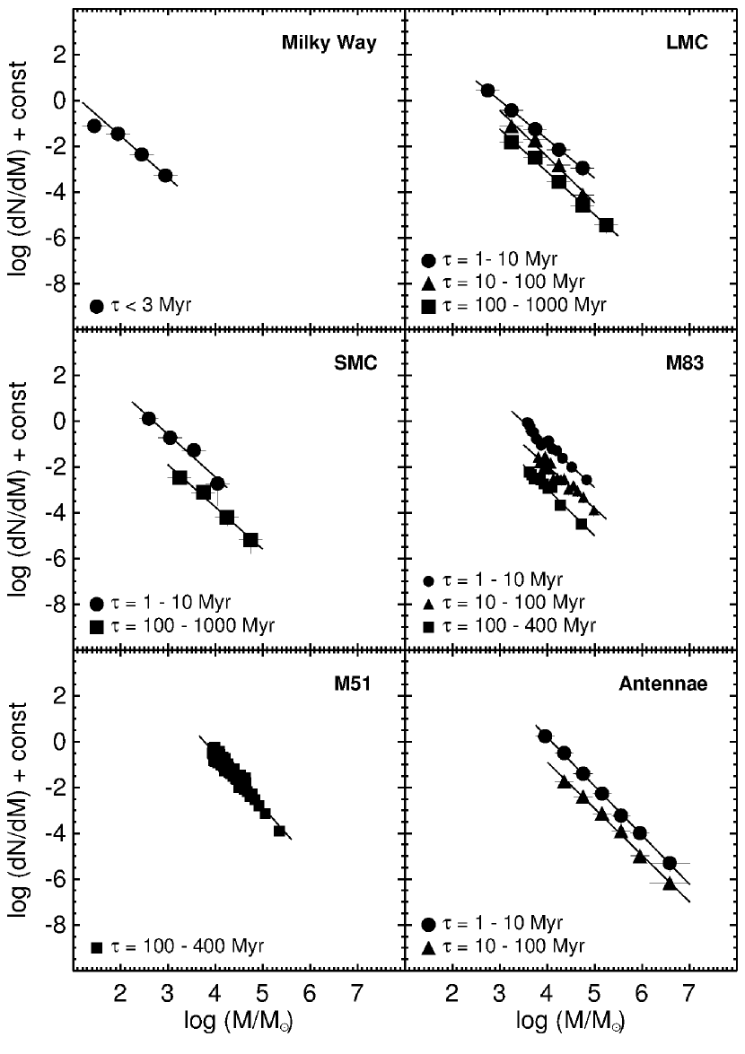
Figure 1: Mass functions of star clusters in different age intervals in different galaxies (as indicated). These have been adapted from the references given in the text. The absolute normalizations of the mass functions are arbitrary, but the relative normalizations within each panel are preserved. The lines show power laws, $dN/dM\propto M^{\beta}$, with the best-fit exponents listed in Table 1. Note that these are all close to $\beta=-1.9$.

Figure 4: Concentration, half-mass radius, and half-mass density plotted against mass for LMC clusters (circles) and SMC clusters (triangles) in two intervals of age (as indicated). All quantities were determined by McLaughlin & van der Marel (2005): $c$, $r_{h}$, and $\rho_{h}$ from fits of King models to HST images and $M$ from total luminosities and mass-to-light ratios inferred from integrated colors and stellar population models. Note that there is a positive correlation between $r_{h}$ and $M$ but none between $c$ and $M$ or between $\rho_{h}$ and $M$.

Table 1: Exponents of Mass Functions

Galaxy	Age Interval	$\beta$
	log($\tau$/yr)
Milky Way	$<$6.5	$-1.82\pm 0.01$
LMC	6$-$7	$-1.70\pm 0.02$
LMC	7$-$8	$-2.02\pm 0.23$
LMC	8$-$9	$-1.87\pm 0.07$
SMC	6$-$7	$-1.87\pm 0.25$
SMC	8$-$9	$-1.84\pm 0.14$
M83	6$-$7	$-1.91\pm 0.10$
M83	7$-$8	$-1.86\pm 0.13$
M83	8$-$8.6	$-2.06\pm 0.13$
M51	8$-$8.6	$-2.24\pm 0.08$
Antennae	6$-$7	$-2.14\pm 0.03$
Antennae	7$-$8	$-2.03\pm 0.07$

Table 2: Exponents of Age Distributions

Galaxy	Mass Interval	$\gamma$
	log($M/M_{\odot}$)
Milky Way	$>2.2$	$-0.97\pm 0.16$
LMC	2.8$-$3.4	$-0.54\pm 0.10$
LMC	3.4$-$4.0	$-0.68\pm 0.07$
LMC	4.0$-$4.8	$-0.75\pm 0.07$
SMC	3.0$-$3.5	$-0.73\pm 0.17$
SMC	3.5$-$4.5	$-0.70\pm 0.16$
M83	3.5$-$4.0	$-0.94\pm 0.09$
M83	$>4.0$	$-0.95\pm 0.09$
Antennae	4.3$-$5.0	$-1.04\pm 0.30$
Antennae	$>5.0$	$-1.05\pm 0.11$

References

- (1) Bastian, N., Adamo, A., Gieles, M., et al. 2012, MNRAS, 419, 2606
- (2) Baumgardt, H., & Kroupa, P. 2007, MNRAS, 380, 1589
- (3) Binney, J., & Tremaine, S. 2008, Galactic Dynamics (2nd ed.; Princeton, NJ: Princeton Univ. Press)
- (4) Blitz, L., Fukui, Y., Kawamura, A., et al. 2007, in Protostars and Planets V, ed. B. Reipurth, D. Jewitt, & K. Keil (Tucson, AZ: Univ. Arizona Press), 81
- (5) Boutloukos, S. G., & Lamers, H. J. G. L. M. 2003, MNRAS, 338, 717
- (6) Chabrier, G. 2003, PASP, 115, 763
- (7) Chandar, R., Fall, S. M., & Whitmore, B. C. 2010a, ApJ, 711, 1263
- (8) Chandar, R., Whitmore, B. C., Calzetti, D., et al. 2011, ApJ, 727, 88
- (9) Chandar, R., Whitmore, B. C., & Fall, S. M. 2010b, ApJ, 713, 1343
- (10) Chandar, R., Whitmore, B. C., Kim, H., et al. 2010c, ApJ, 719, 966
- (11) Chernoff, D. F., & Weinberg, M. D. 1990, ApJ, 351, 121
- (12) de Grijs, R., & Anders, P. 2006, MNRAS, 366, 295
- (13) Fall, S. M. 2006, ApJ, 652, 1129
- (14) Fall, S. M., Chandar, R., & Whitmore, B. C. 2005, ApJ, 631, L133
- (15) Fall, S. M., Chandar, R., & Whitmore, B. C., 2009 ApJ, 704, 453
- (16) Fall, S. M., Krumholz, M. R., & Matzner, C. D. 2010, ApJ, 710, L142
- (17) Fall, S. M., & Zhang, Q. 2001, ApJ, 561, 751
- (18) Faúndez, S., Bronfman, L., Garay, G., et al. 2004, A&A, 426, 97
- (19) Fontani, F., Beltrán, M. T., Brand, J., et al. 2005, A&A, 432, 921
- (20) Fouesneau, M., Lancon, A., Chandar, R., & Whitmore, B. C. 2012, ApJ, 750, 60
- (21) Fukui, Y., Kawamura, A., Minamidani, T., et al. 2008, ApJS, 178, 56
- (22) Fukushige, T., & Heggie, D. C. 1995, MNRAS, 276, 206
- (23) Harris, J., & Zaritsky, D. 2004, AJ, 127, 1531
- (24) Harris, J., & Zaritsky, D. 2009, AJ, 138, 1243
- (25) Karl, S. J., Fall, S. M., & Naab, T. 2011, ApJ, 734, 11
- (26) Krumholz, M. R., & Matzner, C. D. 2009, ApJ, 703, 1352
- (27) Lada, C. J., & Lada, E. A. 2003, ARA&A, 41, 57
- (28) Larsen, S. S. 2009, A&A, 494, 539
- (29) McKee, C. F., & Ostriker, E. C. 2007, ARA&A, 45, 565
- (30) McLaughlin, D. E., & Fall, S. M. 2008, ApJ, 679, 1272
- (31) McLaughlin, D. E., & van der Marel, R. P. 2005, ApJS, 161, 304
- (32) Muñoz, D. J., Mardones, D., Garay, G., et al. 2007, ApJ, 668, 906
- (33) Murray, N., Quataert, E., & Thompson, T. A. 2010, ApJ, 709, 191
- (34) Rosolowsky, E. 2005, PASP, 117, 1403
- (35) Salpeter, E. E. 1955, ApJ, 121, 161
- (36) Shirley, Y. L., Evans, N. J., Young, K. E., Knez, C., & Jaffe, D. T. 2003, ApJS, 149, 375
- (37) Spitzer, L. 1958, ApJ, 127, 17
- (38) Whitmore, B. C., Chandar, R., & Fall, S. M. 2007, AJ, 133, 1067
- (39) Wong, T., Hughes, A., Ott, J., et al. 2011, ApJS, 197, 16
- (40) Wong, T., Ladd, E. F., Brisbin, D., et al. 2008, MNRAS, 386, 1069
- (41) Wu, J., Evans, N. J., Shirley, Y. L., & Knez, C. 2010, ApJS, 188, 313
- (42) Wyse, R. F. G. 2009, in IAU Symp. 258, The Ages of Stars, ed. E. E. Mamajek, D. R. Soderblom, & R. F. G. Wyse (Cambridge: Cambridge Univ. Press), 11