Succinct representations for abstract interpretation
Combined analysis algorithms and experimental evaluation

Abstract.

Abstract interpretation techniques can be made more precise by distinguishing paths inside loops, at the expense of possibly exponential complexity. SMT-solving techniques and sparse representations of paths and sets of paths avoid this pitfall.

We improve previously proposed techniques for guided static analysis and the generation of disjunctive invariants by combining them with techniques for succinct representations of paths and symbolic representations for transitions based on static single assignment.

Because of the non-monotonicity of the results of abstract interpretation with widening operators, it is difficult to conclude that some abstraction is more precise than another based on theoretical local precision results. We thus conducted extensive comparisons between our new techniques and previous ones, on a variety of open-source packages.

1. Introduction

Static analysis by abstract interpretation is a fully automatic program analysis method. When applied to imperative programs, it computes an inductive invariant mapping each program location (or a subset thereof) to a set of states represented symbolically [CousotCousot_JLC92]. For instance, if we are only interested in scalar numerical program variables, such a set may be a convex polyhedron (the set of solutions of a system of linear inequalities) [CousotHalbwachs78, Halbwachs_PhD, PPL, BagnaraHZ08SCP].

In such an analysis, information may flow forward or backward; forward program analysis computes super-sets of the states reachable from the initialization of the program, backward program analysis computes super-sets of the states co-reachable from some property of interest (for instance, the violation of an assertion). In forward analysis, control-flow joins correspond to convex hulls if using convex polyhedra (more generally, they correspond to least upper bounds in a lattice); in backward analysis, it is control-flow splits that correspond to convex hulls.

It is a known limitation of program analysis by abstract interpretation that this convex hull, or more generally, least upper bound operation, may introduce states that cannot occur in the real program: for instance, the convex hull of the intervals $[-2,-1]$ and $[1,2]$ is $[-2,2]$, strictly larger than the union of the two. Such introduction may prevent proving desired program properties, for instance $\neq 0$. The alternative is to keep the union symbolic (e.g. compute using $[-2,-1]\cup[1,2]$) and thus compute in the disjunctive completion of the lattice, but the number of terms in the union may grow exponentially with the number of successive tests in the program to analyze, not to mention difficulties for designing suitable widening operators for enforcing the convergence of fixpoint iterations [PPL, BagnaraHZ08SCP, DBLP:journals/sttt/BagnaraHZ07]. The exponential growth of the number of terms in the union may be controlled by heuristics that judiciously apply least upper bound operations, as in the trace partitioning domain [Rival_Mauborgne_TOPLAS07] implemented in the Astrée analyzer [ASTREE_PLDI03, ASTREE_ESOP05].

Assuming we are interested in a loop-free program fragment, the above approach of keeping symbolic unions gives the same results as performing the analysis separately over every path in the fragment. A recent method for finding disjunctive loop invariants [DBLP:conf/pldi/GulwaniZ10] is based on this idea: each path inside the loop body is considered separately. Two recent proposals use SMT-solving [Kroening_Strichman_08] as a decision procedure for the satisfiability of first-order arithmetic formulas in order to enumerate only paths that are needed for the progress of the analysis [Gawlitza_Monniaux_ESOP11, Monniaux_Gonnord_SAS11]. They can equivalently be seen as analyses over a multigraph of transitions between some distinguished control nodes. This multigraph has an exponential number of edges, but is never explicitly represented in memory; instead, this graph is implicitly or succinctly represented: its edges are enumerated as needed as solutions to SMT problems.

An additional claim in favor of the methods that distinguish paths inside the loop body [DBLP:conf/pldi/GulwaniZ10, Monniaux_Gonnord_SAS11] is that they tend to generate better invariants than methods that do not, by behaving better with respect to the widening operators [CousotCousot_JLC92] used for enforcing convergence when searching for loop invariants by Kleene iterations. A related technique, guided static analysis [DBLP:conf/sas/GopanR07], computes successive loop invariants for increasing subsets of the transitions taken into account, until all transitions are considered; again, the claim is that this approach avoids some gross over-approximation introduced by widenings.

All these methods improve the precision of the analysis by keeping the same abstract domain (say, convex polyhedra) but changing the operations applied and their ordering. An alternative is to change the abstract domain (e.g. octagons, convex polyhedra [DBLP:journals/lisp/Mine06]), or the widening operator [BagnaraHRZ05SCP, Polka:FMSD:97].

This article makes the following contributions:

1. We recast the guided static analysis technique from [DBLP:conf/sas/GopanR07] on the expanded multigraph from [Monniaux_Gonnord_SAS11], considering entire paths instead of individual transitions, using SMT queries and binary decision diagrams (See §3).

2. We improve the technique for obtaining disjunctive invariants from [DBLP:conf/pldi/GulwaniZ10] by replacing the explicit exhaustive enumeration of paths by a sequence of SMT queries (See §LABEL:sec:disjunctive).

3. We implemented these techniques, in addition to “classical” iterations and the original guided static analysis, inside a prototype static analyzer. This tool uses the LLVM bitcode format [Lattner:2004:LCF:977395.977673, LLVM_langref] as input, which can be produced by compilation from C, C++ and Fortran, enabling it to be run on many real-life programs. It uses the APRON library [DBLP:conf/cav/JeannetM09], which supports a variety of abstract domains for numerical variables, from which we can choose with minimal changes to our analyzer.

4. We conducted extensive experiments with this tool, on real-life programs.

2. Bases

2.1. Static Analysis by Abstract Interpretation

Let $X$ be the set of possible states of the program variables; for instance, if the program has 3 unbounded integer variables, then $X=\mathbb{Z}^{3}$. The set $\mathscr{P}(X)$ of subsets of $X$, partially ordered by inclusion, is the concrete domain. An abstract domain is a set $X^{\sharp}$ equipped with a partial order $\sqsubseteq$ (the associated strict order being $\sqsubset$); for instance, it can be the domain of convex polyhedra in $\mathbb{Q}^{3}$ ordered by geometric inclusion. The concrete and abstract domains are connected by a monotone concretization function $\gamma:\left(X^{\sharp},\sqsubseteq\right)\rightarrow(\mathscr{P}(X),\subseteq)$: an element $x^{\sharp}\in X^{\sharp}$ represents a set $\gamma(x^{\sharp})$.

We also assume a join operator $\sqcup:X^{\sharp}\times X^{\sharp}\rightarrow X^{\sharp}$, with infix notation; in practice, it is generally a least upper bound operation, but we only need it to satisfy $\gamma(x^{\sharp})\cup\gamma(y^{\sharp})\subseteq\gamma(x^{\sharp}\sqcup y^{\sharp})$ for all $x^{\sharp},y^{\sharp}$.

Classically, one considers the control-flow graph of the program, with edges labeled with concrete transition relations (e.g. $x^{\prime}=x+1$ for an instruction x = x+1;), and attaches an abstract element to each control point. A concrete transition relation $\tau\subseteq X\times X$ is replaced by an abstract forward abstract transformer $\tau^{\sharp}:X^{\sharp}\rightarrow X^{\sharp}$, such that $\forall x^{\sharp}\in X^{\sharp},x,x^{\prime}\in X,~{}x\in\gamma(x^{\sharp})\land(x,x^{\prime})\in\tau\implies x^{\prime}\in\gamma\circ\tau^{\sharp}(x^{\sharp})$. It is easy to see that if to any control point $p\in P$ we attach an abstract element $x^{\sharp}_{p}$ such that (i) for any $p$, $\gamma(x^{\sharp}_{p})$ includes all initial states possible at control node $p$ (ii) for any $p,p^{\prime}$, $\tau^{\sharp}_{p,p^{\prime}}(x^{\sharp}_{p})\sqsubseteq x^{\sharp}_{p^{\prime}}$, noting $\tau_{p,p^{\prime}}$ the transition from $p$ to $p^{\prime}$, then $(\gamma(x^{\sharp}_{p}))_{p\in P}$ form an inductive invariant: by induction, when the control point is $p$, the program state always lies in $\gamma(x^{\sharp}_{p})$.

Kleene iterations compute such an inductive invariant as the stationary limit, if it exists, of the following system: for each $p$, initialize $x^{\sharp}_{p}$ such that $\gamma(x^{\sharp}_{p})$ is a superset of the initial states at point $p$; then iterate the following: if $\tau^{\sharp}_{p,p^{\prime}}(x^{\sharp}_{p})\not\sqsubseteq x^{\sharp}_{p^{\prime}}$, replace $x^{\sharp}_{p^{\prime}}$ by $x^{\sharp}_{p^{\prime}}\sqcup\tau^{\sharp}_{p,p^{\prime}}(x^{\sharp}_{p})$. Such a stationary limit is bound to exist if $X^{\sharp}$ has no infinite ascending chain $a_{1}\sqsubset a_{2}\sqsubset\dots$; this condition is however not met by domains such as intervals or convex polyhedra.

Widening-accelerated Kleene iterations proceed by replacing $x^{\sharp}_{p^{\prime}}\sqcup\tau^{\sharp}_{p,p^{\prime}}(x^{\sharp}_{p})$ by $x^{\sharp}_{p^{\prime}}\mathop{\triangledown}(x^{\sharp}_{p^{\prime}}\sqcup\tau^{\sharp}_{p,p^{\prime}}(x^{\sharp}_{p}))$ where $\mathop{\triangledown}$ is a widening operator: for all $x^{\sharp},y^{\sharp}$, $\gamma(y^{\sharp})\subseteq\gamma(x^{\sharp}\mathop{\triangledown}y^{\sharp})$, and any sequence $u^{\sharp}_{1},u^{\sharp}_{2},\dots$ of the form $u^{\sharp}_{n+1}=u^{\sharp}_{n}\mathop{\triangledown}v^{\sharp}_{n}$, where $v^{\sharp}_{n}$ is another sequence, become stationary. The stationary limit $(x^{\sharp}_{p})_{p\in P}$, defines an inductive invariant $(\gamma(x^{\sharp}_{p}))_{p\in P}$. Note that this invariant is not, in general, the least one expressible in the abstract domain, and may depend on the iteration ordering (the successive choices $p,p^{\prime}$).

Once an inductive invariant $\gamma((x^{\sharp}_{p})_{p\in P})$ has been obtained, one can attempt decreasing or narrowing iterations to reduce it. In their simplest form, this just means running the following operation until a fixpoint or a maximal number of iterations are reached: for any $p^{\prime}$, replace $x^{\sharp}_{p^{\prime}}$ by $x^{\sharp}_{p^{\prime}}\cap\left(\bigsqcup_{p\in P}\tau^{\sharp}_{p,p^{\prime}}(x^{\sharp}_{p})\right)$. The result also defines an inductive invariant. These decreasing iterations are indispensable to recover properties from guards (tests) in the program in most iteration settings; unfortunately, certain loops, particularly those involving identity (no-operation) transitions, may foil them: the iterations immediately reach a fixpoint and do not decrease further (see example in §2.3). Sections 2.4 and 2.5 describe techniques that work around this problem.

2.2. SMT-solving

Boolean satisfiability (SAT) is the canonical NP-complete problem: given a propositional formula (e.g. $(a\lor\neg b)\land(\neg a\lor b\lor\neg c)$), decide whether it is satisfiable — and, if so, output a satisfying assignment. Despite an exponential worst-case complexity, the DPLL algorithm [Kroening_Strichman_08, Handbook_SAT] solves many useful SAT problems in practice.

SAT was extended to satisfiability modulo theory (SMT): in addition to propositional literals, SMT formulas admit atoms from a theory. For instance, the theories of linear integer arithmetic (LIA) and linear real arithmetic (LRA) have atoms of the form $a_{1}x_{1}+\dots+a_{n}x_{n}\bowtie C$ where $a_{1},\dots,a_{n},C$ are integer constants, $x_{1},\dots,x_{n}$ are variables (interpreted over $\mathbb{Z}$ for LIA and $\mathbb{R}$ or $\mathbb{Q}$ for LRA), and $\bowtie$ is a comparison operator $=,\neq,<,\leq,>,\geq$. Satisfiability for LIA and LRA is NP-complete, yet tools based on DPLL(T) approach [Kroening_Strichman_08, Handbook_SAT] solve many useful SMT problems in practice. All these tools provide a satisfying assignment if the problem is satisfiable.

2.3. A Simple, Motivating Example

Consider the following program, adapted from [Monniaux_Gonnord_SAS11], where input($a$, $b$) stands for a nondeterministic input in $[a,b]$ (the control-flow graph on the right depicts the loop body, $s$ is the start node and $e$ the end node):

⬇

1void rate_limiter() {

2 int x_old = 0;

3 while (1) {

4 int x = input(-100000, 100000);

5 if (x > x_old+10) x = x_old+10;

6 if (x < x_old-10) x = x_old-10;

7 x_old = x;

8} }

This program implements a construct commonly found in control programs (in e.g. automotive or avionics): a rate or slope limiter.

The expected inductive invariant is ${\leavevmode\lstinline{{\lst@@@set@language\lst@@@set@numbers\lst@@@set@frame\lst@@@set@rulecolor\lst@@@set@language\lst@@@set@numbers\rm\small{\@listingGroup{ltx_lst_identifier}{x\textunderscore old}}}}}\in[-100000,100000]$, but classical abstract interpretation using intervals (or octagons or polyhedra) finds ${\leavevmode\lstinline{{\lst@@@set@language\lst@@@set@numbers\lst@@@set@frame\lst@@@set@rulecolor\lst@@@set@language\lst@@@set@numbers\rm\small{\@listingGroup{ltx_lst_identifier}{x\textunderscore old}}}}}\in(-\infty,+\infty)$ [ASTREE_ESOP05]. Let us briefly see why.

Widening iterations converge to ${\leavevmode\lstinline{{\lst@@@set@language\lst@@@set@numbers\lst@@@set@frame\lst@@@set@rulecolor\lst@@@set@language\lst@@@set@numbers\rm\small{\@listingGroup{ltx_lst_identifier}{x\textunderscore old}}}}}\in(-\infty,+\infty)$; let us now see why decreasing iterations fail to recover the desired invariant. The x > x_old+10 test at line 6, if taken, yields ${\leavevmode\lstinline{{\lst@@@set@language\lst@@@set@numbers\lst@@@set@frame\lst@@@set@rulecolor\lst@@@set@language\lst@@@set@numbers\rm\small{\@listingGroup{ltx_lst_identifier}{x\textunderscore old}}}}}\in(-\infty,99990)$; followed by x = x_old+10, we obtain ${\leavevmode\lstinline{{\lst@@@set@language\lst@@@set@numbers\lst@@@set@frame\lst@@@set@rulecolor\lst@@@set@language\lst@@@set@numbers\rm\small{\@listingGroup{ltx_lst_identifier}{x}}}}}\in(-\infty,\allowbreak 100000)$, and the same after union with the no-operation “else” branch. Line 7 yields ${\leavevmode\lstinline{{\lst@@@set@language\lst@@@set@numbers\lst@@@set@frame\lst@@@set@rulecolor\lst@@@set@language\lst@@@set@numbers\rm\small{\@listingGroup{ltx_lst_identifier}{x}}}}}\in(-\infty,+\infty)$.

We could use “widening up to” or “widening with thresholds”, propagating the “magic values” $\pm 100000$ associated to x into x_old, but these syntactic approaches cannot directly cope with programs for which ${\leavevmode\lstinline{{\lst@@@set@language\lst@@@set@numbers\lst@@@set@frame\lst@@@set@rulecolor\lst@@@set@language\lst@@@set@numbers\rm\small{\@listingGroup{ltx_lst_identifier}{x}}}}}\in[-100000,+100000]$ is itself obtained by analysis. The guided static analysis of [DBLP:conf/sas/GopanR07] does not perform better, and also obtains ${\leavevmode\lstinline{{\lst@@@set@language\lst@@@set@numbers\lst@@@set@frame\lst@@@set@rulecolor\lst@@@set@language\lst@@@set@numbers\rm\small{\@listingGroup{ltx_lst_identifier}{x\textunderscore old}}}}}\in(-\infty,+\infty)$.

In contrast, let us distinguish all four possible execution paths through the tests at lines 6 and 7. The path through both “else” branches is infeasible; the program is thus equivalent to a program with 3 paths:

⬇

1void rate_limiter() {

2 int x_old = 0;

3 while (1) {

4 int x = input(-100000, 100000);

5 if (x > x_old+10) x_old = x_old+10;

6 else if (x < x_old-10) x_old = x_old-10;

7 else x_old = x;

8} }

Classical interval analysis on this program yields ${\leavevmode\lstinline{{\lst@@@set@language\lst@@@set@numbers\lst@@@set@frame\lst@@@set@rulecolor\lst@@@set@language\lst@@@set@numbers\rm\small{\@listingGroup{ltx_lst_identifier}{x\textunderscore old}}}}}\in[-100000,100000]$. We have transformed the program, manually pruning out infeasible paths; yet in general the resulting program could be exponentially larger than the first, even though not all feasible paths are needed to compute the invariant.

Following recent suggestions [Gawlitza_Monniaux_ESOP11, Monniaux_Gonnord_SAS11], we avoid this space explosion by keeping the second program implicit while simulating its analysis. This means we work on an implicitly represented transition multigraph ; it is succinctly represented by the transition graph of the first program. Our first contribution (§3) is to recast the “guided analysis” from [DBLP:conf/sas/GopanR07] on such a succinct representation of the paths in lieu of the individual transitions. A similar explosion occurs in disjunctive invariant generation, following [DBLP:conf/pldi/GulwaniZ10]; our second contribution (§LABEL:sec:disjunctive) applies our implicit representation to their method.

2.4. Guided Static Analysis

Guided static analysis was proposed by [DBLP:conf/sas/GopanR07] as an improvement over classical upward Kleene iterations with widening. Consider the program in Fig. 1, taken from [DBLP:conf/sas/GopanR07].

⬇

1int x = 0, y = 0;

2while (1) {

3 if (x <= 50) y++;

4 else y–;

5 if (y < 0) break;

6 x++;

7}

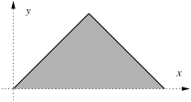
$$y\leq x\;\land\;y\leq 102-x\;\land\;y\geq 0.$$

Figure 1. Example program and its invariant: the piecewise linear, solid line is the strongest invariant, the grayed polyhedron is its convex hull.

Classical iterations on the domain of convex polyhedra [CousotHalbwachs78, BagnaraHRZ05SCP] or octagons [DBLP:journals/lisp/Mine06] start with $x=0\land x=0$, then continue with $x=y\land 0\leq x\leq 1$. The widening operator extrapolates from these two iterations and yields $x=y\land x\geq 0$. From there, the “else” branch at line 4 may be taken; with further widening, $0\leq y\leq x$ is obtained as a loop invariant, and thus the computed loop postcondition is $x\geq 0\land y=0$. Yet the strongest invariant is $(0\leq x\leq 51\land y=x)\lor(51\leq x\leq 102\land x+y=102)$, and its convex hull, a convex polyhedron (Fig. 1).

Intuitively, this disappointing result is obtained because widening extrapolates from the first iterations of the loop, but the loop has two different phases ($x\leq 50$ and $x>50$) with different behaviors, thus the extrapolation from the first phase is not valid for the second.

Gopan and Reps’ idea is to analyze the first phase of the loop with a widening and narrowing sequence, and thus obtain $0\leq x\leq 50\land y=x$, and then analyze the second phase, finally obtaining invariant (1); each phase is identified by the tests taken or not taken.

The analysis starts by identifying the tests taken and not taken during the first iteration of the loop, starting in the loop initialization. The branches not taken are pruned from the loop body, yielding:

⬇

while(1) {

if(x <= 50) y++;

else break; /* not taken in phase 1 */

if(y < 0) break;

x++;

}

Analyzing this loop using widening and narrowing on convex polyhedra or octagons yields the loop invariant $0\leq x\leq 51\land y=x$. Now, the transition at line 4 becomes feasible; and we analyze the full loop, starting iterations from $0\leq x\leq 51\land y=x$, and obtain invariant (1) in Fig 1.

More generally, this analysis method considers an ascending sequence of subsets of the transitions in the loop body ; for each subset, an inductive invariant is computed for the program restricted to it. The starting subset consists in the transitions reachable in one step from the loop initialization. If for a given subset $S$ in the sequence, no transitions outside $S$ are reachable from the inductive invariant attached to $S$, then iterations stop; otherwise, add these transitions to $S$ and iterate more. Termination ensues from the finiteness of the control-flow graph.

2.5. Path-focusing

Monniaux & Gonnord’s path-focusing [Monniaux_Gonnord_SAS11] technique distinguishes the different paths in the program in order to avoid loss of precision due to merge operations. Since the number of paths may be exponential, the technique keeps them implicit and computes them when needed using SMT-solving. The (accelerated) Kleene iterations (§2.1) are computed over a reduced multigraph instead of the classical transition graph.

Let $P$ be the set of control points in the transition graph, $P_{W}\subseteq P$ the set of widening points such that removing the points in $P_{W}$ gives an acyclic graph. One can choose a set $P_{R}$ such that $P_{W}\subseteq P_{R}\subseteq P$.

The set of paths is kept implicit by an SMT formula $\rho$ expressing the semantics of the program, assuming that the transition semantics can be expressed within a decidable theory. For an easy construction of $\rho$, we also assume that the program is expressed in SSA form, meaning that each variable is only assigned once in the transition graph. This is not a restriction, since there exists standard algorithms that transform a program into an SSA format.

This formula contains Boolean reachability predicates $b_{i}$ for each control points $p_{i}\notin P_{R}$, $b_{i}^{s}$ and $b_{i}^{d}$ for each $p_{i}\in P_{R}$, so that a path $p_{i_{1}}\rightarrow p_{i_{2}}\rightarrow\dots\rightarrow p_{i_{n}}$ between two points $p_{i_{1}},p_{i_{n}}\in P_{R}$ can easily be expressed as the conjunction $b_{i_{1}}^{s}\wedge\bigwedge_{2\leq k<n}b_{i_{k}}\wedge b_{i_{n}}^{d}$. The Boolean $b_{i}^{s}$ is $true$ when the path starts at point $p_{i}$, whereas $b_{i}^{d}$ is $true$ when the path arrives at $p_{i}$. In other words, we split the points in $P_{R}$ into a source point, with only outgoing transitions, and a destination point, with only incoming transitions, so that the resulting graph is acyclic and there are no paths going through control points in $P_{R}$.

In order to find focus paths, we solve an SMT formula which is satisfiable when there exists a path starting at a point $p_{i}\in P_{R}$ in a state included in the current invariant candidate $X_{i}$, and arriving at a point $p_{j}\in P_{R}$ in a state outside $X_{j}$. In this case, we construct this path using the model and update $X_{j}$. When $p_{i}=p_{j}$, meaning that the path is actually a self-loop, we can apply a widening/narrowing sequence, or even compute the transitive closure of the loop (or an approximation thereof, or its application to $X_{i}$) using abstract acceleration [DBLP:conf/sas/GonnordH06].

We assume that we can encode the concrete semantics of the program into the SMT formula, or at least an abstraction thereof at least as precise as the one applied by the abstract interpreter (in simple terms: we want to avoid the case where the SMT solver exhibits a possible path, but the static analyzer realizes that this path is infeasible; this would lead to nontermination, because the SMT solver would exhibit the same path on the next iteration). A workaround would be to apply satisfiability modulo path programs [DBLP:conf/popl/HarrisSIG10]: from each path ruled infeasible by abstract interpretation, extract a blocking clause for the SAT solver underlying the SMT-solver.

3. Guided Analysis over the Paths

Guided static analysis, as proposed by [DBLP:conf/sas/GopanR07], applies to the transition graph of the program. We now present a new technique applying this analysis on the implicit multigraph from [Monniaux_Gonnord_SAS11], thus avoiding control flow merges with unfeasible paths. In this section, we use the same notations as §2.5.

The combination of these two techniques aims at first discovering a precise inductive invariant for a subset of paths between two points in $P_{R}$, by the mean of ascending and narrowing iterations. When an inductive invariant has been found, we add new feasible paths to the subset and compute an inductive invariant for this new subset, starting with the results from the previous analysis. In other words, our technique considers an ascending sequence of subsets of the paths between two points in $P_{R}$. We iterate the operations until the whole program (i.e all the feasible paths) has been considered. The result will then be an inductive invariant of the entire program.

The ascending iteration applies path-focusing [Monniaux_Gonnord_SAS11] to a subset of the multigraph. As [DBLP:conf/sas/GopanR07], we do some narrowing, to recover precision lost by widening, before computing and taking into account new feasible paths. Thus, our technique combines the advantages of Guided Static Analysis and Path-focusing.

Algorithm 1 performs Guided static analysis on the implicitly represented multigraph. $I_{p}$ denotes a set of initial states at program point $p$ (thus $\emptyset$ for most $p$). The current working subset of paths, noted $P$ and initially empty, is stored using a compact representation, such as binary decision diagrams. We also maintain two sets of control points:

• $A^{\prime}$ : points in $P_{R}$ that may be the starting points of new feasible paths.

• $A$ : points in $P_{R}$ on which we apply the ascending iterations. When the abstract value of a control point $p$ is updated, $p$ is added to both $A$ and $A^{\prime}$.

Algorithm 1 Guided static analysis on implicit multigraph

1:  $A^{\prime}\leftarrow\{p|P_{R}/I_{p}\neq\emptyset\}$

2:  $A\leftarrow\emptyset$

3:  $P\leftarrow\emptyset$ // Paths in the current subset

4:  for all $p_{i}\in P_{R}$ do

5:     $X_{i}\leftarrow I_{p_{i}}$

6:  end for

7:  while $A^{\prime}\neq\emptyset$ do

8:     while $A^{\prime}\neq\emptyset$ do

9:        Select $p_{i}\in A^{\prime}$

10:        $A^{\prime}\leftarrow A^{\prime}\setminus\{p_{i}\}$

11:        ComputeNewPaths($p_{i}$) // Update $A$, $A^{\prime}$ and $P$

12:     end while

13:      // ascending iterations on $P$

14:     while $A\neq\emptyset$ do

15:        Select $p_{i}\in A$

16:        $A\leftarrow A\setminus\{p_{i}\}$

17:        PathFocusing($p_{i}$) // Update $A$ and $A^{\prime}$

18:     end while

19:     Narrow

20:  end while

21:  return  $\{X_{i},\ i\in P_{R}\}$

We distinguish three phases in the main loop of the analysis:

1. We start finding a new relevant subset $P$ of the graph. Either the previous iteration or the initialization led us to a state where there are no more paths in the previous subset $P$, starting at $p_{i}$, that make the abstract values of the successors grow (otherwise, the SMT solver would not have answered “unsat”). Narrowing iterations preserve this property. However, there may exist such paths in the entire multigraph, that are not in $P$. This phase computes these paths and adds them to the subset. This phase is described in 3.2 and corresponds to lines in 8 to 12 in Algorithm 1.

2. Given a new subset $P$, we search for paths starting at point $p_{i}\in P_{R}$, such that these paths are in $P$, i.e are included in the working subgraph. Each time we find a path, we update the abstract value of the destination point of the path. This is the phase explained in 3.1, and corresponds to lines 14 to 18 in Algorithm 1.

3. We perform narrowing iterations the usual way (line 19 in algorithm 1) and reiterate from step 1 unless there are no more points to explore, i.e. $A^{\prime}=\emptyset$.

The order of steps is important: narrowing has to be performed before adding new paths, or spurious new paths would be added to $P$. Starting with the addition of new paths avoids doing the ascending iterations on an empty graph.

3.1. Ascending Iterations by Path-focusing

For computing an inductive invariant over a subgraph, we use the Path-focusing algorithm from [Monniaux_Gonnord_SAS11] with special treatment for self loops (line 17 in algorithm 1).

In order to find which path to focus on, we construct an SMT formula $f(p_{i})$, whose model when satisfiable is a path that starts in $p_{i}$, goes to a successor $p_{j}\in P_{R}$ of $p_{i}$, such that the image of $X_{i}$ by the path transformation is not included in the current $X_{j}$. Intuitively, such a path makes the abstract value $X_{j}$ grow, and thus is an interesting path to focus on. We loop until the formula becomes unsatisfiable, meaning that the analysis of $p_{i}$ is finished.

If we note $Succ(i)$ the set of indices $j$ such that $p_{j}\in P_{R}$ is a successor of $p_{i}$ in the expanded multigraph, and $X_{i}$ the abstract value associated to $p_{i}$ :

$$f(p_{i})=\rho\wedge b_{i}^{s}\wedge\displaystyle\bigwedge_{j\in P_{R}\atop j\neq i}\neg b_{j}^{s}\wedge X_{i}\wedge\displaystyle\bigvee_{j\in Succ(i)}(b_{j}^{d}\wedge\neg X_{j})$$

The difference with [Monniaux_Gonnord_SAS11] is that we do not work on the entire transition graph but on a subset of it. Therefore we conjoin the formula $f(p_{i})$ with the actual set of working paths, noted $P$, expressed as a Boolean formula, where the Boolean variables are the reachability predicates of the control points. We can easily construct this formula from the binary decision diagram using dynamic programming, and avoiding an exponentially sized formula. In other words, we force the SMT solver to give us a path included in $P$. Each time the invariant candidate of a point $p_{j}$ has been updated, $p_{j}$ is inserted into $A^{\prime}$ since it may be the start of a new feasible paths.

3.2. Adding New Paths

Our technique computes the fixpoint iterations on an ascending sequence of subgraphs, until the complete graph is reached. When the analysis of a subgraph is finished, meaning that the abstract values for each control point has converged to an inductive invariant for this subgraph, the next subgraph to work on has to be computed.

This new subgraph contains all the paths from the previous one, and also new paths that become feasible regarding the current abstract values. The new paths in $P$ are computed one after another, until no more path can make the invariant grow. This is line 11 in Algorithm 1, which corresponds to Algorithm 2. We also use SMT solving to discover these new paths, but we subtly change the SMT formula given to the SMT solver: we now try to find a path that is not yet in $P$, but is feasible and makes the invariant candidate of its destination grow. We thus check the satisfiability of the formula $f^{\prime}(p_{i})$, where:

$$f^{\prime}(p_{i})=f(p_{i})\wedge\neg P$$

$X_{j}$ is updated using an abstract union when the point $p_{j}$ is the target of a new path. This way, further SMT queries do not compute other paths with the same source and destination if it is not needed (because these new paths would not make $X_{j}$ grow, hence would not be returned by the SMT solver).

Algorithm 2 ComputeNewPaths

1:  while true do

2:     $res\leftarrow SmtSolve\left[f^{\prime}(p_{i})\right]$

3:     if $res=unsat$ then

4:        break

5:     end if

6:     Compute the path $e$ from the model

7:     $X_{j}\leftarrow X_{j}\sqcup\tau_{e}(X_{i})$

8:     $P\leftarrow P\cup\{e\}$

9:     $A\leftarrow A\cup\{p_{i}\}$

10:     $A^{\prime}\leftarrow A^{\prime}\cup\{p_{i}\}$

11:  end while

When a new path has been found, it is immediately added into $P$. We then have to add $p_{i}$ and $p_{j}$ into $A$ (since we do not apply widening in this section) and $p_{j}$ into $A^{\prime}$, since $p_{j}$ may be the starting point of a new feasible path.

3.3. Termination

Termination of this algorithm is guaranteed, because: (1) the subset of paths $P$ strictly increases at each loop iteration, and is bounded by the finite set of paths in the entire graph. (2) when computing new paths, we cunjunct our formula with $\neg P$, meaning that we obtain each possible path only once. The number of path is finite, so this computation always terminates. (3) the Path-focusing iterations terminate because of the properties of widening.

3.4. Example

We revise the rate limiter described in 2.3. In this example, Path-focusing works well because all the paths starting at the loop header are actually self loops. In such a case, the technique performs a widening/narrowing sequence or accelerates the loop, thus leading to a precise invariant. However, in some cases, there also exists paths that are not self loops, in which case Path-focusing applies widening. This widening may induce unrecoverable loss of precision.

Suppose the main loop of the rate limiter contains a nested loop like:

⬇

1void rate_limiter() {

2 int x_old = 0;

3 while (1) {

4 int x = input(-100000, 100000);

5 if (x > x_old+10) x = x_old+10;

6 if (x < x_old-10) x = x_old-10;

7 x_old = x;

8 while (wait()) {}

9} }

We choose $P_{R}$ as the set of loop headers of the function, plus the initial state. In this case, we have three elements in $P_{R}$.

The main loop in the expanded multigraph has then 4 distinct paths going to the header of the nested loop.

Guided static analysis from [DBLP:conf/sas/GopanR07] yields, at line 3, ${\leavevmode\lstinline{{\lst@@@set@language\lst@@@set@numbers\lst@@@set@frame\lst@@@set@rulecolor\lst@@@set@language\lst@@@set@numbers\rm\small{\@listingGroup{ltx_lst_identifier}{x\textunderscore old}}}}}\in(-\infty,+\infty)$. Path-focusing [Monniaux_Gonnord_SAS11] also finds ${\leavevmode\lstinline{{\lst@@@set@language\lst@@@set@numbers\lst@@@set@frame\lst@@@set@rulecolor\lst@@@set@language\lst@@@set@numbers\rm\small{\@listingGroup{ltx_lst_identifier}{x\textunderscore old}}}}}\in(-\infty,+\infty)$. Now, let us see how our technique performs on this example.

Figure LABEL:fig:example-graph shows the sequence of subset of paths during the analysis. The points in $P_{R}$ are noted $p_{i}$, where $i$ is the corresponding line in the code: for instance, $p_{3}$ corresponds to the header of the main loop.

1. The starting subgraph is depicted on Figure LABEL:fig:example-graph Step 1. At the beginning, this graph has no transitions.

2. We compute the new feasible paths that have to be added into the subgraph. We first find the path from $p_{1}$ to $p_{3}$ and obtain at $p_{3}$ ${\leavevmode\lstinline{{\lst@@@set@language\lst@@@set@numbers\lst@@@set@frame\lst@@@set@rulecolor\lst@@@set@language\lst@@@set@numbers\rm\small{\@listingGroup{ltx_lst_identifier}{x\textunderscore old}}}}}=0$.

   The image of ${\leavevmode\lstinline{{\lst@@@set@language\lst@@@set@numbers\lst@@@set@frame\lst@@@set@rulecolor\lst@@@set@language\lst@@@set@numbers\rm\small{\@listingGroup{ltx_lst_identifier}{x\textunderscore old}}}}}=0$ by the path that goes from $p_{3}$ to $p_{8}$, and that goes through the else branch of each if-then-else, is ${-10\leq\leavevmode\lstinline{{\lst@@@set@language\lst@@@set@numbers\lst@@@set@frame\lst@@@set@rulecolor\lst@@@set@language\lst@@@set@numbers\rm\small{\@listingGroup{ltx_lst_identifier}{x\textunderscore old}}}}}\leq 10$. This path is then added to our subgraph.

   Moreover, there is no other path starting at $p_{3}$ whose image is not in ${-10\leq\leavevmode\lstinline{{\lst@@@set@language\lst@@@set@numbers\lst@@@set@frame\lst@@@set@rulecolor\lst@@@set@language\lst@@@set@numbers\rm\small{\@listingGroup{ltx_lst_identifier}{x\textunderscore old}}}}}\leq 10$.

   Finally, since the abstract value associated to $p_{8}$ is ${-10\leq\leavevmode\lstinline{{\lst@@@set@language\lst@@@set@numbers\lst@@@set@frame\lst@@@set@rulecolor\lst@@@set@language\lst@@@set@numbers\rm\small{\@listingGroup{ltx_lst_identifier}{x\textunderscore old}}}}}\leq 10$, the path from $p_{8}$ to $p_{3}$ is feasible and is added into $P$. The final subgraph is depicted on Figure LABEL:fig:example-graph Step 2.

3. We then compute the ascending iterations by path-focusing. At the end of these iterations, we obtain ${-\infty\leq\leavevmode\lstinline{{\lst@@@set@language\lst@@@set@numbers\lst@@@set@frame\lst@@@set@rulecolor\lst@@@set@language\lst@@@set@numbers\rm\small{\@listingGroup{ltx_lst_identifier}{x\textunderscore old}}}}}\leq+\infty$ for both $p_{3}$ and $p_{8}$.

4. We now can apply narrowing iterations, and recover the precision lost by widening: we obtain ${-10000\leq\leavevmode\lstinline{{\lst@@@set@language\lst@@@set@numbers\lst@@@set@frame\lst@@@set@rulecolor\lst@@@set@language\lst@@@set@numbers\rm\small{\@listingGroup{ltx_lst_identifier}{x\textunderscore old}}}}}\leq 10000$ at points $p_{3}$ and $p_{8}$.

5. Finally, we compute the next subgraph. The SMT-solver does not find any new path that makes the abstract values grow, and the algorithm terminates.

Our technique gives us the expected invariant ${\leavevmode\lstinline{{\lst@@@set@language\lst@@@set@numbers\lst@@@set@frame\lst@@@set@rulecolor\lst@@@set@language\lst@@@set@numbers\rm\small{\@listingGroup{ltx_lst_identifier}{x\textunderscore old}}}}}\in~{}[-10000,\allowbreak 10000]$. Here, only 3 paths out of the 6 have been computed during the analysis. In practice, depending on the order the SMT-solver returns the paths, other feasible paths could have been added during the analysis.