Model-based clustering via
linear cluster-weighted models

Abstract

A novel family of twelve mixture models with random covariates, nested in the linear $t$ cluster-weighted model (CWM), is introduced for model-based clustering. The linear $t$ CWM was recently presented as a robust alternative to the better known linear Gaussian CWM. The proposed family of models provides a unified framework that also includes the linear Gaussian CWM as a special case. Maximum likelihood parameter estimation is carried out within the EM framework, and both the BIC and the ICL are used for model selection. A simple and effective hierarchical random initialization is also proposed for the EM algorithm. The novel model-based clustering technique is illustrated in some applications to real data. Finally, a simulation study for evaluating the performance of the BIC and the ICL is presented.

1 Introduction

In direct applications of finite mixture models (see Titterington et al., 1985, pp. 2–3), we assume that each mixture-component represents a group (or cluster) in the original data. The term ``model-based clustering'' has been used to describe the adoption of mixture models for clustering or, more often, to describe the use of a family of mixture models for clustering (see Fraley & Raftery, 1998 and McLachlan & Basford, 1988). An overview of mixture models is given in Everitt & Hand (1981), Titterington et al. (1985), McLachlan & Peel (2000), and Frühwirth-Schnatter (2006).

This paper focuses on data arising from a real-valued random vector $\left(Y,\boldsymbol{X}^{\prime}\right)^{\prime}:\Omega\rightarrow\text{\rm IR}^{d+1}$, having joint density $p\left(y,\boldsymbol{x}\right)$, where $Y$ is the response variable and $\boldsymbol{X}$ is the vector of covariates. Standard model-based clustering techniques assume that $\Omega$ can be partitioned into $G$ groups $\Omega_{1},\ldots,\Omega_{G}$. As for finite mixtures of linear regressions (see, e.g., Leisch, 2004 and Frühwirth-Schnatter, 2006, Chapter 8) we assume that, for each $\Omega_{g}$, the dependence of $Y$ on $\boldsymbol{x}$ can be modeled by

$$Y=\mu\left(\boldsymbol{x};\mbox{\boldmath$\beta$}_{g}\right)+\varepsilon_{g}=\beta_{0g}+\mbox{\boldmath$\beta$}_{1g}^{\prime}\boldsymbol{x}+\varepsilon_{g},$$

where $\mbox{\boldmath$\beta$}_{g}=\left(\beta_{0g},\mbox{\boldmath$\beta$}_{1g}^{\prime}\right)^{\prime}$, $\mu\left(\boldsymbol{x};\mbox{\boldmath$\beta$}_{g}\right)=E\left(Y|\boldsymbol{X}=\boldsymbol{x},\Omega_{g}\right)$ is the linear regression function and $\varepsilon_{g}$ is the error variable, independent with respect to $\boldsymbol{X}$, with zero mean and finite constant variance $\sigma_{g}^{2}$, $g=1,\ldots,G$. However, as highlighted in Hennig (2000), finite mixtures of linear regressions are inadequate for most of the applications because they assume assignment independence: the probability for a point $\left(y,\boldsymbol{x}^{\prime}\right)^{\prime}$ to be generated by one of the mixture components has to be the same for all covariates values $\boldsymbol{x}$. In other words, the assignment of the data points to the clusters has to be independent of the covariates.

Here, differently from finite mixtures of linear regressions, we assume random covariates having a parametric specification. This allows for assignment dependence: the covariate distributions of the mixture components can also be distinct. In the framework of mixture models with random covariates, the cluster weighted model (CWM; Gershenfeld, 1997), with equation

$$p\left(y,\boldsymbol{x}\right)=\sum_{g=1}^{G}\pi_{g}p\left(y,\boldsymbol{x}|\Omega_{g}\right)=\sum_{g=1}^{G}\pi_{g}p\left(y|\boldsymbol{x},\Omega_{g}\right)p\left(\boldsymbol{x}|\Omega_{g}\right),$$ (1)

also called saturated mixture regression model by Wedel (2002), constitutes a reference approach to model the joint density. In (1), normality of both $p\left(y|\boldsymbol{x},\Omega_{g}\right)$ and $p\left(\boldsymbol{x}|\Omega_{g}\right)$ is commonly assumed (see, e.g., Gershenfeld, 1997 and Punzo, 2014). Alternatively, Ingrassia et al. (2012) propose also the use of the $t$ distribution which provides, as other approaches (Punzo & McNicholas, 2013, 2014a, 2014b), more robust fitting for groups of observations with longer than normal tails or noise data (see, e.g., Zellner, 1976, Lange et al., 1989, Peel & McLachlan, 2000, McLachlan & Peel, 2000, Chapter 7, Chatzis & Varvarigou, 2008, and Greselin & Ingrassia, 2010). In particular, the authors consider

$$p\left(y|\boldsymbol{x},\Omega_{g}\right)=h_{t}\left(y|\boldsymbol{x};\mbox{\boldmath$\xi$}_{g},\zeta_{g}\right)=\frac{\Gamma\left(\displaystyle\frac{\zeta_{g}+1}{2}\right)}{\left(\pi\zeta_{g}\sigma^{2}_{g}\right)^{\frac{1}{2}}\left\{1+\delta\left[y,\mu\left(\boldsymbol{x};\mbox{\boldmath$\beta$}_{g}\right);\sigma^{2}_{g}\right]\right\}^{\frac{\zeta_{g}+1}{2}}}$$ (2)

and

$$p\left(\boldsymbol{x}|\Omega_{g}\right)=h_{t_{d}}\left(\boldsymbol{x};\boldsymbol{\vartheta}_{g},\nu_{g}\right)=\frac{\Gamma\left(\displaystyle\frac{\nu_{g}+d}{2}\right)\left|\mbox{\boldmath$\Sigma$}_{g}\right|^{-\frac{1}{2}}}{\left(\pi\nu_{g}\right)^{\frac{d}{2}}\left[1+\delta\left(\boldsymbol{x},\mbox{\boldmath$\mu$}_{g};\mbox{\boldmath$\Sigma$}_{g}\right)\right]^{\frac{\nu_{g}+d}{2}}},$$ (3)

with $\mbox{\boldmath$\xi$}_{g}=\left\{\mbox{\boldmath$\beta$}_{g},\sigma^{2}_{g}\right\}$, $\boldsymbol{\vartheta}_{g}=\left\{\mbox{\boldmath$\mu$}_{g},\mbox{\boldmath$\Sigma$}_{g}\right\}$, $\delta\left[y,\mu(\boldsymbol{x};\mbox{\boldmath$\beta$}_{g});\sigma^{2}_{g}\right]=\left[y-\mu\left(\boldsymbol{x};\mbox{\boldmath$\beta$}_{g}\right)\right]^{2}\big{/}\sigma^{2}_{g}$, and $\delta\left(\boldsymbol{x},\mbox{\boldmath$\mu$}_{g};\mbox{\boldmath$\Sigma$}_{g}\right)=\left(\boldsymbol{x}-\mbox{\boldmath$\mu$}_{g}\right)^{\prime}\mbox{\boldmath$\Sigma$}_{g}^{-1}\left(\boldsymbol{x}-\mbox{\boldmath$\mu$}_{g}\right)$. Thus, (2) is the density of a (generalized) univariate $t$ distribution, with location parameter $\mu\left(\boldsymbol{x};\mbox{\boldmath$\beta$}_{g}\right)$, scale parameter $\sigma^{2}_{g}$, and $\zeta_{g}$ degrees of freedom, while (3) is the density of a multivariate $t$ distribution with location parameter $\mbox{\boldmath$\mu$}_{g}$, inner product matrix $\mbox{\boldmath$\Sigma$}_{g}$, and $\nu_{g}$ degrees of freedom. By substituting (2) and (3) into (1), we obtain the linear $t$ CWM

$$p\left(y,\boldsymbol{x};\text{{$\boldsymbol{\psi}$}}\right)=\sum_{g=1}^{G}\pi_{g}h_{t}\left(y|\boldsymbol{x};\mbox{\boldmath$\xi$}_{g},\zeta_{g}\right)h_{t_{d}}\left(\boldsymbol{x};\mbox{\boldmath$\vartheta$}_{g},\nu_{g}\right),$$ (4)

where the set of all unknown parameters is denoted by $\text{{$\boldsymbol{\psi}$}}=\left\{\mbox{\boldmath$\psi$}_{1},\ldots,\mbox{\boldmath$\psi$}_{G}\right\}$, with $\mbox{\boldmath$\psi$}_{g}=\left\{\pi_{g},\mbox{\boldmath$\xi$}_{g},\zeta_{g},\boldsymbol{\vartheta}_{g},\nu_{g}\right\}$. Recent developments in CWMs can be found in Punzo (2014), Punzo & McNicholas (2014a), Punzo & Ingrassia (2015a, b), Subedi et al. (2013, 2015), and Ingrassia et al. (2015).

In this paper, we introduce a family of twelve linear CWMs obtained from (4) by imposing convenient component distributional constraints. If $\zeta_{g},\nu_{g}\rightarrow\infty$, the linear Gaussian (normal) CWM is obtained as a special case. The resulting models are easily interpretable and appropriate for describing various practical situations. In particular, they also allow us to infer if the group-structure of the data is due to the contribution of $\boldsymbol{X}$, $Y|\boldsymbol{X}$, or both.

The paper is organized as follows. In Section 2, we recall model-based clustering according to the CW approach, and give some preliminary results. In Section 3, we introduce the novel family of models. Model fitting in the EM paradigm is presented in Section 4, related computational aspects are addressed in Section 5, and model selection is discussed in Section 6. In Section 7 some applications to real data are illustrated. In Section 8 simulations for a comparison between BIC and ICL are described. Finally, in Section 9, we give a summary of the paper and some directions for further research.

2 Preliminary results for model-based clustering

This section recalls some basic ideas on model-based clustering according to the CWM approach and provides some preliminary results that will be useful for definition and justification of our family of models.

Let $\left(y_{1},\boldsymbol{x}_{1}^{\prime}\right)^{\prime},\ldots,\left(y_{N},\boldsymbol{x}_{N}^{\prime}\right)^{\prime}$ be a sample of size $N$ from (4). Once $\psi$ is estimated (fixed), the posterior probability that the generic unit $\left(y_{n},\boldsymbol{x}_{n}^{\prime}\right)^{\prime}$, $n=1,\ldots,N$, comes from component $\Omega_{g}$ is given by

$$\tau_{ng}=P\left(\Omega_{g}|y_{n},\boldsymbol{x}_{n};{\mbox{\boldmath$\psi$}}\right)=\frac{\pi_{g}h_{t}\left(y_{n}|\boldsymbol{x}_{n};\mbox{\boldmath$\xi$}_{g},\zeta_{g}\right)h_{t_{d}}\left(\boldsymbol{x}_{n};\mbox{\boldmath$\vartheta$}_{g},\nu_{g}\right)}{p\left(y_{n},\boldsymbol{x}_{n};{\mbox{\boldmath$\psi$}}\right)},\quad g=1,\ldots,G.$$ (5)

These probabilities, which depend on both marginal and conditional densities, represent the basis for clustering and classification.

The following two propositions, which generalize some results given in Ingrassia et al. (2012), require the preliminary definition of

$$p\left(y|\boldsymbol{x};\text{{$\pi$}},\text{{$\boldsymbol{\xi}$}},\text{{$\zeta$}}\right)=\sum_{g=1}^{G}\pi_{g}h_{t}\left(y|\boldsymbol{x};\mbox{\boldmath$\xi$}_{g},\zeta_{g}\right)$$ (6)

and

$$p\left(\boldsymbol{x};\text{{$\pi$}},\text{{$\boldsymbol{\vartheta}$}},\text{{$\nu$}}\right)=\sum_{g=1}^{G}\pi_{g}h_{t_{d}}\left(\boldsymbol{x};\mbox{\boldmath$\vartheta$}_{g},\nu_{g}\right),$$ (7)

which correspond to a finite mixture of linear $t$ regressions and a finite mixture of multivariate $t$ distributions ($\text{{$\pi$}}=\left\{\pi_{1},\ldots,\pi_{G-1}\right\}$, $\text{{$\boldsymbol{\xi}$}}=\left\{\xi_{1},\ldots,\xi_{G}\right\}$, $\text{{$\zeta$}}=\left\{\zeta_{1},\ldots,\zeta_{G}\right\}$, $\text{{$\boldsymbol{\vartheta}$}}=\left\{\vartheta_{1},\ldots,\vartheta_{G}\right\}$, and $\text{{$\nu$}}=\left\{\nu_{1},\ldots,\nu_{G}\right\}$), respectively .

Proposition 1.

Given $\pi$, $\boldsymbol{\vartheta}$, and $\nu$, if $h_{t}\left(y|\boldsymbol{x};\mbox{\boldmath$\xi$}_{1},\zeta_{1}\right)=\cdots=h_{t}\left(y|\boldsymbol{x};\mbox{\boldmath$\xi$}_{G},\zeta_{G}\right)=h_{t}\left(y|\boldsymbol{x};\mbox{\boldmath$\xi$},\zeta\right)$, then models (4) and (7) generate the same posterior probabilities.

Proof 1.

If the component conditional densities do not depend on $\Omega_{g}$, then the posterior probabilities for the linear $t$ CWM in (4) can be written as

$$\tau_{ng}=\frac{\pi_{g}\cancel{h_{t}\left(y_{n}|\boldsymbol{x}_{n};\mbox{\boldmath$\xi$},\zeta\right)}h_{t_{d}}\left(\boldsymbol{x}_{n};\mbox{\boldmath$\vartheta$}_{g},\nu_{g}\right)}{\displaystyle\sum_{j=1}^{G}\pi_{j}\cancel{h_{t}\left(y_{n}|\boldsymbol{x}_{n};\mbox{\boldmath$\xi$},\zeta\right)}h_{t_{d}}\left(\boldsymbol{x}_{n};\mbox{\boldmath$\vartheta$}_{j},\nu_{j}\right)}=\frac{\pi_{g}h_{t_{d}}\left(\boldsymbol{x}_{n};\mbox{\boldmath$\vartheta$}_{g},\nu_{g}\right)}{\displaystyle\sum_{j=1}^{G}\pi_{j}h_{t_{d}}\left(\boldsymbol{x}_{n};\mbox{\boldmath$\vartheta$}_{j},\nu_{j}\right)},$$

which correspond to the posterior probabilities for model (7).∎

Proposition 2.

Given $\pi$, $\boldsymbol{\xi}$, and $\zeta$, if $h_{t_{d}}\left(\boldsymbol{x};\mbox{\boldmath$\vartheta$}_{1},\nu_{1}\right)=\cdots=h_{t_{d}}\left(\boldsymbol{x};\mbox{\boldmath$\vartheta$}_{G},\nu_{G}\right)=h_{t_{d}}\left(\boldsymbol{x};\mbox{\boldmath$\vartheta$},\nu\right)$, then models (4) and (6) generate the same posterior probabilities.

Proof 2.

If the component marginal densities do not depend on $\Omega_{g}$, then the posterior probabilities for the linear $t$ CWM in (4) can be written as

$$\tau_{ng}=\frac{\pi_{g}h_{t}\left(y_{n}|\boldsymbol{x}_{n};\mbox{\boldmath$\xi$}_{g},\zeta_{g}\right)\cancel{h_{t_{d}}\left(\boldsymbol{x}_{n};\mbox{\boldmath$\vartheta$},\nu\right)}}{\displaystyle\sum_{j=1}^{G}\pi_{j}h_{t}\left(y_{n}|\boldsymbol{x}_{n};\mbox{\boldmath$\xi$}_{j},\zeta_{j}\right)\cancel{h_{t_{d}}\left(\boldsymbol{x}_{n};\mbox{\boldmath$\vartheta$},\nu\right)}}=\frac{\pi_{g}h_{t}\left(y_{n}|\boldsymbol{x}_{n};\mbox{\boldmath$\xi$}_{g},\zeta_{g}\right)}{\displaystyle\sum_{j=1}^{G}\pi_{j}h_{t}\left(y_{n}|\boldsymbol{x}_{n};\mbox{\boldmath$\xi$}_{j},\zeta_{j}\right)},$$

which correspond to the posterior probabilities for model (6).∎

Note that the results in Proposition 1 and 2 are not restricted to the $t$ distribution; in fact, they can be easily extended to the general CWM in (1). Further, some results about the relation between linear Gaussian (or $t$) CWMs and finite mixture of regressions are given in Ingrassia et al. (2012). Finally, it is important to underline that up to now there are no theoretical results on the identifiability for linear CWMs; however, since they can be seen as mixture models with random covariates, the results in Hennig (2000, Section 3, Model 2.a) can apply.

3 The family of linear CWMs

This section introduces the novel family of mixture models obtained from the linear $t$ CWM. In (4), let us consider:

• component conditional densities $h_{t}$ having the same parameters for all $\Omega_{g}$,

• component marginal densities $h_{t_{d}}$ having the same parameters for all $\Omega_{g}$,

• degrees of freedom $\zeta_{g}$ tending to infinity for each $\Omega_{g}$, and

• degrees of freedom $\nu_{g}$ tending to infinity for each $\Omega_{g}$.

By combining such constraints, we obtain twelve parsimonious and easily interpretable linear CWMs that are appropriate for describing various practical situations; they are schematically presented in Table 1 along with the number of parameters characterizing each component of the CW decomposition. For instance, if $\nu_{g},\zeta_{g}\rightarrow\infty$ for each $\Omega_{g}$, we are assuming a normal distribution for the component conditional and marginal densities; furthermore, we can assume different linear models (in terms of $\mbox{\boldmath$\beta$}_{g}$ and $\sigma^{2}_{g}$) in each cluster while keeping the density of $\boldsymbol{X}$ equal between clusters. From a notational viewpoint, this leads to a linear CWM that we have simply denoted as $NN$-EV: the first two letters represent the distribution of $\boldsymbol{X}|\Omega_{g}$ and $Y|\boldsymbol{X},\Omega_{g}$ ($N\equiv$Normal and $t\equiv$$t$), respectively, while the second two denote the distribution constraint between clusters (E$\equiv$Equal and V$\equiv$Variable) for $\boldsymbol{X}|\Omega_{g}$ and $Y|\boldsymbol{X},\Omega_{g}$, respectively.

Model	$\boldsymbol{X}|\Omega_{g}$		$Y|\boldsymbol{x},\Omega_{g}$		Number of free parameters
Identifier	Density	Constraint	Density	Constraint	$\boldsymbol{X}$		$Y|\boldsymbol{x}$		weights
$tt$-VV	$t$	Variable	$t$	Variable	$G\left(d+\frac{d\left(d+1\right)}{2}+1\right)$	+	$G\left(d+3\right)$	+	$G-1$
$tt$-VE	$t$	Variable	$t$	Equal	$G\left(d+\frac{d\left(d+1\right)}{2}+1\right)$	+	$d+3$	+	$G-1$
$tt$-EV	$t$	Equal	$t$	Variable	$d+\frac{d\left(d+1\right)}{2}+1$	+	$G\left(d+3\right)$	+	$G-1$
$NN$-VV	Normal	Variable	Normal	Variable	$G\left(d+\frac{d\left(d+1\right)}{2}\right)$	+	$G\left(d+2\right)$	+	$G-1$
$NN$-VE	Normal	Variable	Normal	Equal	$G\left(d+\frac{d\left(d+1\right)}{2}\right)$	+	$d+2$	+	$G-1$
$NN$-EV	Normal	Equal	Normal	Variable	$d+\frac{d\left(d+1\right)}{2}$	+	$G\left(d+2\right)$	+	$G-1$
$tN$-VV	$t$	Variable	Normal	Variable	$G\left(d+\frac{d\left(d+1\right)}{2}+1\right)$	+	$G\left(d+2\right)$	+	$G-1$
$tN$-VE	$t$	Variable	Normal	Equal	$G\left(d+\frac{d\left(d+1\right)}{2}+1\right)$	+	$d+2$	+	$G-1$
$tN$-EV	$t$	Equal	Normal	Variable	$d+\frac{d\left(d+1\right)}{2}+1$	+	$G\left(d+2\right)$	+	$G-1$
$Nt$-VV	Normal	Variable	$t$	Variable	$G\left(d+\frac{d\left(d+1\right)}{2}\right)$	+	$G\left(d+3\right)$	+	$G-1$
$Nt$-VE	Normal	Variable	$t$	Equal	$G\left(d+\frac{d\left(d+1\right)}{2}\right)$	+	$d+3$	+	$G-1$
$Nt$-EV	Normal	Equal	$t$	Variable	$d+\frac{d\left(d+1\right)}{2}$	+	$G\left(d+3\right)$	+	$G-1$

Table 1: Overview of linear CWMs. In ``model identifier'', the first and second letters represent, respectively, the density of $\boldsymbol{X}|\Omega_{g}$ and $Y|\boldsymbol{x},\Omega_{g}$ (here $N\equiv$Normal), while the third and fourth letters indicate, respectively, if $h_{t_{d}}\left(\boldsymbol{x};\mbox{\boldmath$\vartheta$}_{g},\nu_{g}\right)$ and $h_{t}\left(y|\boldsymbol{x};\mbox{\boldmath$\xi$}_{g},\zeta_{g}\right)$ are assumed to be Equal$\equiv$E or Variable$\equiv$V between groups.

Only two of the models given in Table 1, $NN$-VV and $tt$-VV, have been developed previously; the former corresponds to the linear Gaussian CWM of Gershenfeld (1997), while the latter coincides with the linear $t$ CWM in Ingrassia et al. (2012). Furthermore, in principle there are sixteen models arising from the combination of the aforementioned constraints; nevertheless, four of them – those which should be denoted as EE – do not make sense. Indeed, they lead to a single cluster regardless of the value of $G$. Finally, we remark that when $G=1$, it results $\text{VV}\equiv\text{VE}\equiv\text{EV}$ regardless of the chosen distribution.

4 Estimation via the EM algorithm

The EM algorithm (Dempster et al., 1977) is the standard tool for maximum likelihood (ML) estimation of the parameters for mixture models. This section describes the EM algorithm for the most general model $tt$-VV. Details for all the other models are given in A.

In the EM framework, the generic observation $\left(y_{n},\boldsymbol{x}_{n}^{\prime}\right)^{\prime}$ is viewed as being incomplete; its complete counterpart is given by $\left(y_{n},\boldsymbol{x}_{n}^{\prime},\boldsymbol{z}_{n}^{\prime},u_{n},v_{n}\right)^{\prime}$, where $\boldsymbol{z}_{n}$ is the component-label vector in which $z_{ng}=1$ if $\left(y_{n},\boldsymbol{x}_{n}^{\prime}\right)^{\prime}$ comes from the $g$th component ($z_{ng}=0$ otherwise), while $u_{n}$ and $v_{n}$ arise from the standard theory of the (multivariate) $t$ distribution according to which

$$Y_{n}\left|\boldsymbol{x}_{n},v_{n},z_{ng}=1\right. \stackrel{{\scriptstyle\text{ind.}}}{{\sim}} \text{N}\left(\mu\left(\boldsymbol{x}_{n};\mbox{\boldmath$\beta$}_{g}\right),\frac{\sigma^{2}_{g}}{v_{n}}\right)$$ (8)

$$V_{n}\left|z_{ng}=1\right. \stackrel{{\scriptstyle\text{i.i.d.}}}{{\sim}} \text{Gamma}\left(\frac{\zeta_{g}}{2},\frac{\zeta_{g}}{2}\right),$$ (9)

for $n=1,\ldots,N$, and

$$\boldsymbol{X}_{n}\left|u_{n},z_{ng}=1\right. \stackrel{{\scriptstyle\text{ind.}}}{{\sim}} \text{N}\left(\mbox{\boldmath$\mu$}_{g},\frac{\mbox{\boldmath$\Sigma$}_{g}}{u_{n}}\right)$$ (10)

$$U_{n}\left|z_{ng}=1\right. \stackrel{{\scriptstyle\text{i.i.d.}}}{{\sim}} \text{Gamma}\left(\frac{\nu_{g}}{2},\frac{\nu_{g}}{2}\right),$$ (11)

for $n=1,\ldots,N$. Because of the conditional structure of the complete-data model given by distributions (8), (9), (10), and (11), the complete-data log-likelihood can be decomposed as

$$l_{c}\left(\text{{$\boldsymbol{\psi}$}}\right)=l_{1c}\left(\text{{$\pi$}}\right)+l_{2c}\left(\text{{$\boldsymbol{\xi}$}}\right)+l_{3c}\left(\text{{$\zeta$}}\right)+l_{4c}\left(\text{{$\boldsymbol{\vartheta}$}}\right)+l_{5c}\left(\text{{$\nu$}}\right),$$ (12)

where

$$l_{1c}\left(\text{{$\pi$}}\right)=\sum_{n=1}^{N}\sum_{g=1}^{G}z_{ng}\ln\pi_{g},$$

$$l_{2c}\left(\text{{$\boldsymbol{\xi}$}}\right)=\frac{1}{2}\sum_{n=1}^{N}\sum_{g=1}^{G}z_{ng}\Bigl{\{}-\ln\left(2\pi\right)+\ln v_{n}-\ln\sigma^{2}_{g}-v_{n}\delta\left[y_{n},\mu\left(\boldsymbol{x}_{n};\mbox{\boldmath$\beta$}_{g}\right);\sigma^{2}_{g}\right]\Bigr{\}},$$

$$l_{3c}\left(\text{{$\zeta$}}\right)=\sum_{n=1}^{N}\sum_{g=1}^{G}z_{ng}\left[-\ln\Gamma\left(\frac{\zeta_{g}}{2}\right)+\frac{\zeta_{g}}{2}\ln\frac{\zeta_{g}}{2}+\frac{\zeta_{g}}{2}\left(\ln v_{n}-v_{n}\right)-\ln v_{n}\right],$$

$$l_{4c}\left(\text{{$\boldsymbol{\vartheta}$}}\right)=\frac{1}{2}\sum_{n=1}^{N}\sum_{g=1}^{G}z_{ng}\left[-d\ln\left(2\pi\right)+d\ln u_{n}-\ln\left|\mbox{\boldmath$\Sigma$}_{g}\right|-u_{n}\delta\left(\boldsymbol{x}_{n},\mbox{\boldmath$\mu$}_{g};\mbox{\boldmath$\Sigma$}_{g}\right)\right]$$

and

$$l_{5c}\left(\text{{$\nu$}}\right)=\sum_{n=1}^{N}\sum_{g=1}^{G}z_{ng}\left[-\ln\Gamma\left(\frac{\nu_{g}}{2}\right)+\frac{\nu_{g}}{2}\ln\frac{\nu_{g}}{2}+\frac{\nu_{g}}{2}\left(\ln u_{n}-u_{n}\right)-\ln u_{n}\right].$$

4.1 E-step

The E-step, on the $\left(k+1\right)$th iteration, requires the calculation of

$$Q\left(\text{{$\boldsymbol{\psi}$}};\text{{$\boldsymbol{\psi}$}}^{\left(k\right)}\right)=E_{\text{{$\boldsymbol{\psi}$}}^{\left(k\right)}}\left[l_{c}\left(\text{{$\boldsymbol{\psi}$}}\right)\left|\left(y_{1},\boldsymbol{x}_{1}^{\prime}\right)^{\prime},\ldots,\left(y_{n},\boldsymbol{x}_{n}^{\prime}\right)^{\prime}\right.\right].$$ (13)

In order to do this, we need to calculate $E_{\text{{$\boldsymbol{\psi}$}}^{\left(k\right)}}\left(Z_{ng}\left|y_{n},\boldsymbol{x}_{n}\right.\right)$, $E_{\text{{$\boldsymbol{\psi}$}}^{\left(k\right)}}\left(V_{n}\left|y_{n},\boldsymbol{x}_{n},\boldsymbol{z}_{n}\right.\right)$, $E_{\text{{$\boldsymbol{\psi}$}}^{\left(k\right)}}\left(\widetilde{V}_{n}\left|y_{n},\boldsymbol{x}_{n},\boldsymbol{z}_{n}\right.\right)$, $E_{\text{{$\boldsymbol{\psi}$}}^{\left(k\right)}}\left(U_{n}\left|\boldsymbol{x}_{n},\boldsymbol{z}_{n}\right.\right)$, and $E_{\text{{$\boldsymbol{\psi}$}}^{\left(k\right)}}\left(\widetilde{U}_{n}\left|\boldsymbol{x}_{n},\boldsymbol{z}_{n}\right.\right)$, for $n=1,\ldots,N$ and $g=1,\ldots,G$, where $\widetilde{U}_{n}=\ln U_{n}$ and $\widetilde{V}_{n}=\ln V_{n}$. It follows that

$$E_{\text{{$\boldsymbol{\psi}$}}^{\left(k\right)}}\left(Z_{ng}\left|y_{n},\boldsymbol{x}_{n}\right.\right) = \tau_{ng}^{\left(k\right)}$$ (14)

$$= \frac{\pi_{g}^{\left(k\right)}h_{t}\left(y_{n}|\boldsymbol{x}_{n};\boldsymbol{\xi}_{g}^{\left(k\right)},\zeta_{g}^{\left(k\right)}\right)h_{t_{d}}\left(\boldsymbol{x}_{n};\boldsymbol{\vartheta}_{g}^{\left(k\right)},\nu_{g}^{\left(k\right)}\right)}{p\left(y_{n},\boldsymbol{x}_{n};\text{{$\boldsymbol{\psi}$}}^{\left(k\right)}\right)},$$

$$E_{\text{{$\boldsymbol{\psi}$}}^{\left(k\right)}}\left(V_{n}\left|y_{n},\boldsymbol{x}_{n},z_{ng}=1\right.\right) = v_{ng}^{\left(k\right)}$$ (15)

$$= \frac{\zeta_{g}^{\left(k\right)}+1}{\zeta_{g}^{\left(k\right)}+\delta\left[y_{n},\mu\left(\boldsymbol{x}_{n};\mbox{\boldmath$\beta$}_{g}^{\left(k\right)}\right);\sigma^{2\left(r\right)}_{g}\right]}$$

and

$$E_{\text{{$\boldsymbol{\psi}$}}^{\left(k\right)}}\left(U_{n}\left|y_{n},\boldsymbol{x}_{n},z_{ng}=1\right.\right) = u_{ng}^{\left(k\right)}$$ (16)

$$= \frac{\nu_{g}^{\left(k\right)}+d}{\nu_{g}^{\left(k\right)}+\delta\left(\boldsymbol{x}_{n},\mbox{\boldmath$\mu$}_{g}^{\left(k\right)};\mbox{\boldmath$\Sigma$}_{g}^{\left(k\right)}\right)},$$

where the expectations are affected (see the subscript) using the current fit $\text{{$\boldsymbol{\psi}$}}^{\left(k\right)}$ for $\boldsymbol{\psi}$ ($n=1,\ldots,N$ and $g=1,\ldots,G$). Regarding the last two expectations, from the standard theory on the gamma distribution, we have that

$$E_{\text{{$\boldsymbol{\psi}$}}^{\left(k\right)}}\left(\widetilde{V}_{n}\left|y_{n},\boldsymbol{x}_{n},z_{ng}=1\right.\right) = \widetilde{v}_{ng}^{\left(k\right)}$$ (17)

$$= \ln v_{ng}^{\left(k\right)}+\psi\left(\frac{\zeta_{g}^{\left(k\right)}+1}{2}\right)-\ln\left(\frac{\zeta_{g}^{\left(k\right)}+1}{2}\right)$$

and

$$E_{\text{{$\boldsymbol{\psi}$}}^{\left(k\right)}}\left(\widetilde{U}_{n}\left|\boldsymbol{x}_{n},z_{ng}=1\right.\right) = \widetilde{u}_{ng}^{\left(k\right)}$$ (18)

$$= \ln u_{ng}^{\left(k\right)}+\psi\left(\frac{\nu_{g}^{\left(k\right)}+d}{2}\right)-\ln\left(\frac{\nu_{g}^{\left(k\right)}+d}{2}\right),$$

where $\psi\left(s\right)=\left[\partial\Gamma\left(s\right)/\partial s\right]/\Gamma\left(s\right)$ is the Digamma function.

Using the results from (14) to (17) to calculate (13), we have that

$$Q\left(\text{{$\boldsymbol{\psi}$}};\text{{$\boldsymbol{\psi}$}}^{\left(k\right)}\right)=Q_{1}\left(\text{{$\pi$}};\text{{$\boldsymbol{\psi}$}}^{\left(k\right)}\right)+Q_{2}\left(\text{{$\boldsymbol{\xi}$}};\text{{$\boldsymbol{\psi}$}}^{\left(k\right)}\right)+Q_{3}\left(\text{{$\zeta$}};\text{{$\boldsymbol{\psi}$}}^{\left(k\right)}\right)+Q_{4}\left(\text{{$\boldsymbol{\vartheta}$}};\text{{$\boldsymbol{\psi}$}}^{\left(k\right)}\right)+Q_{5}\left(\text{{$\nu$}};\text{{$\boldsymbol{\psi}$}}^{\left(k\right)}\right),$$ (19)

where

$$Q_{1}\left(\text{{$\pi$}};\text{{$\boldsymbol{\psi}$}}^{\left(k\right)}\right)=\sum_{n=1}^{N}\sum_{g=1}^{G}\tau_{ng}^{\left(k\right)}\ln\pi_{g},$$ (20)

$$Q_{2}\left(\text{{$\boldsymbol{\xi}$}};\text{{$\boldsymbol{\psi}$}}^{\left(k\right)}\right)=\sum_{n=1}^{N}\sum_{g=1}^{G}\tau_{ng}^{\left(k\right)}Q_{2n}\left(\boldsymbol{\xi}_{g};\text{{$\boldsymbol{\psi}$}}^{\left(k\right)}\right),$$ (21)

$$Q_{3}\left(\text{{$\zeta$}};\text{{$\boldsymbol{\psi}$}}^{\left(k\right)}\right)=\sum_{n=1}^{N}\sum_{g=1}^{G}\tau_{ng}^{\left(k\right)}Q_{3n}\left(\zeta_{g};\text{{$\boldsymbol{\psi}$}}^{\left(k\right)}\right),$$ (22)

$$Q_{4}\left(\text{{$\boldsymbol{\vartheta}$}};\text{{$\boldsymbol{\psi}$}}^{\left(k\right)}\right)=\sum_{n=1}^{N}\sum_{g=1}^{G}\tau_{ng}^{\left(k\right)}Q_{4n}\left(\boldsymbol{\vartheta}_{g};\text{{$\boldsymbol{\psi}$}}^{\left(k\right)}\right)$$ (23)

and

$$Q_{5}\left(\text{{$\nu$}};\text{{$\boldsymbol{\psi}$}}^{\left(k\right)}\right)=\sum_{n=1}^{N}\sum_{g=1}^{G}\tau_{ng}^{\left(k\right)}Q_{5n}\left(\nu_{g};\text{{$\boldsymbol{\psi}$}}^{\left(k\right)}\right),$$ (24)

with

$$Q_{2n}\left(\boldsymbol{\xi}_{g};\text{{$\boldsymbol{\psi}$}}^{\left(k\right)}\right)=\frac{1}{2}\left\{-\ln\left(2\pi\right)+\widetilde{v}_{ng}^{\left(k\right)}-\ln\sigma^{2}_{g}-v_{ng}\delta\left[y_{n},\mu\left(\boldsymbol{x}_{n};\mbox{\boldmath$\beta$}_{g}\right);\sigma^{2}_{g}\right]\right\}$$

and

$$Q_{4n}\left(\boldsymbol{\vartheta}_{g};\text{{$\boldsymbol{\psi}$}}^{\left(k\right)}\right)=\frac{1}{2}\left[-d\ln\left(2\pi\right)+d\widetilde{u}_{ng}^{\left(k\right)}-\ln\left|\mbox{\boldmath$\Sigma$}_{g}\right|-u_{ng}\delta\left(\boldsymbol{x}_{n},\mbox{\boldmath$\mu$}_{g};\mbox{\boldmath$\Sigma$}_{g}\right)\right],$$

and where, on ignoring terms not involving $\zeta_{g}$ and $\nu_{g}$, respectively,

$$Q_{3n}\left(\zeta_{g};\text{{$\boldsymbol{\psi}$}}^{\left(k\right)}\right)=-\ln\Gamma\left(\frac{\zeta_{g}}{2}\right)+\frac{\zeta_{g}}{2}\ln\frac{\zeta_{g}}{2}+\frac{\zeta_{g}}{2}\left[\widetilde{v}_{ng}^{\left(k\right)}-\ln v_{ng}^{\left(k\right)}+\sum_{n=1}^{N}\left(\ln v_{ng}^{\left(k\right)}-v_{ng}^{\left(k\right)}\right)\right]$$

and

$$Q_{5n}\left(\nu_{g};\text{{$\boldsymbol{\psi}$}}^{\left(k\right)}\right)=-\ln\Gamma\left(\frac{\nu_{g}}{2}\right)+\frac{\nu_{g}}{2}\ln\frac{\nu_{g}}{2}+\frac{\nu_{g}}{2}\left[\widetilde{u}_{ng}^{\left(k\right)}-\ln u_{ng}^{\left(k\right)}+\sum_{n=1}^{N}\left(\ln u_{ng}^{\left(k\right)}-u_{ng}^{\left(k\right)}\right)\right].$$

4.2 M-step

On the M-step, at the $\left(k+1\right)$th iteration, it follows from (19) that $\text{{$\pi$}}^{\left(k+1\right)}$, $\text{{$\boldsymbol{\xi}$}}^{\left(k+1\right)}$, $\text{{$\zeta$}}^{\left(k+1\right)}$, $\text{{$\boldsymbol{\vartheta}$}}^{\left(k+1\right)}$, and $\text{{$\nu$}}^{\left(k+1\right)}$ can be computed independently of each other, by separate consideration of (20), (21), (22), (23), and (24), respectively. The solutions for $\pi_{g}^{\left(k+1\right)}$, $\boldsymbol{\xi}_{g}^{\left(k+1\right)}$, and $\boldsymbol{\vartheta}_{g}^{\left(k+1\right)}$ exist in closed form. Only the updates $\zeta_{g}^{\left(k+1\right)}$ and $\nu_{g}^{\left(k+1\right)}$ need to be computed iteratively.

The updated estimates of the mixture weights are

$$\pi_{g}^{\left(k+1\right)}=\sum_{n=1}^{N}\tau_{ng}^{\left(k\right)}\Big{/}n,$$ (25)

while those of $\boldsymbol{\vartheta}_{g}$, $g=1,\ldots,G$, result

$$\mbox{\boldmath$\mu$}_{g}^{\left(k+1\right)}=\displaystyle\sum_{n=1}^{N}\tau_{ng}^{\left(k\right)}u_{ng}^{\left(k\right)}\boldsymbol{x}_{n}\Big{/}\displaystyle\sum_{n=1}^{N}\tau_{ng}^{\left(k\right)}u_{ng}^{\left(k\right)}$$ (26)

and

$$\mbox{\boldmath$\Sigma$}_{g}^{\left(k+1\right)}=\displaystyle\sum_{n=1}^{N}\tau_{ng}^{\left(k\right)}u_{ng}^{\left(k\right)}\left(\boldsymbol{x}_{n}-\mbox{\boldmath$\mu$}_{g}^{\left(k+1\right)}\right)\left(\boldsymbol{x}_{n}-\mbox{\boldmath$\mu$}_{g}^{\left(k+1\right)}\right)^{\prime}\Big{/}\displaystyle\sum_{n=1}^{N}\tau_{ng}^{\left(k\right)}u_{ng}^{\left(k\right)},$$ (27)

where, as motivated for example in Shoham (2002), the true denominator $\sum_{n}\tau_{ng}^{\left(k\right)}$ of (27) has been changed to yield a significantly faster convergence for the EM algorithm.

Regarding the updated estimates of $\boldsymbol{\xi}_{g}$, $g=1,\ldots,G$, maximization of (21), after some algebra, yields

$$\mbox{\boldmath$\beta$}_{1g}^{\left(k+1\right)} = \left(\frac{\displaystyle\sum_{n=1}^{N}\tau_{ng}^{\left(k\right)}v_{ng}^{\left(k\right)}\boldsymbol{x}_{n}\boldsymbol{x}_{n}^{\prime}}{\displaystyle\sum_{n=1}^{N}\tau_{ng}^{\left(k\right)}v_{ng}^{\left(k\right)}}-\frac{\displaystyle\sum_{n=1}^{N}\tau_{ng}^{\left(k\right)}v_{ng}^{\left(k\right)}\boldsymbol{x}_{n}}{\displaystyle\sum_{n=1}^{N}\tau_{ng}^{\left(k\right)}v_{ng}^{\left(k\right)}}\frac{\displaystyle\sum_{n=1}^{N}\tau_{ng}^{\left(k\right)}v_{ng}^{\left(k\right)}\boldsymbol{x}_{n}^{\prime}}{\displaystyle\sum_{n=1}^{N}\tau_{ng}^{\left(k\right)}v_{ng}^{\left(k\right)}}\right)^{-1}\cdot$$ (28)

$$\cdot\left(\frac{\displaystyle\sum_{n=1}^{N}\tau_{ng}^{\left(k\right)}v_{ng}^{\left(k\right)}y_{n}\boldsymbol{x}_{n}}{\displaystyle\sum_{n=1}^{N}\tau_{ng}^{\left(k\right)}v_{ng}^{\left(k\right)}}-\frac{\displaystyle\sum_{n=1}^{N}\tau_{ng}^{\left(k\right)}v_{ng}^{\left(k\right)}y_{n}}{\displaystyle\sum_{n=1}^{N}\tau_{ng}^{\left(k\right)}v_{ng}^{\left(k\right)}}\frac{\displaystyle\sum_{n=1}^{N}\tau_{ng}^{\left(k\right)}v_{ng}^{\left(k\right)}\boldsymbol{x}_{n}}{\displaystyle\sum_{n=1}^{N}\tau_{ng}^{\left(k\right)}v_{ng}^{\left(k\right)}}\right),$$

$$\beta_{0g}^{\left(k+1\right)}=\displaystyle\frac{\displaystyle\sum_{n=1}^{N}\tau_{ng}^{\left(k\right)}v_{ng}^{\left(k\right)}y_{n}}{\displaystyle\sum_{n=1}^{N}\tau_{ng}^{\left(k\right)}v_{ng}^{\left(k\right)}}-\mbox{\boldmath$\beta$}_{1g}^{\left(k+1\right)^{\prime}}\frac{\displaystyle\sum_{n=1}^{N}\tau_{ng}^{\left(k\right)}v_{ng}^{\left(k\right)}\boldsymbol{x}_{n}}{\displaystyle\sum_{n=1}^{N}\tau_{ng}^{\left(k\right)}v_{ng}^{\left(k\right)}}$$ (29)

and

$$\sigma^{2\left(k+1\right)}_{g}=\displaystyle\displaystyle\sum_{n=1}^{N}\tau_{ng}^{\left(k\right)}v_{ng}^{\left(k\right)}\left[y_{n}-\left(\beta_{0g}^{\left(k+1\right)}+\boldsymbol{\beta}_{1g}^{\left(k+1\right)^{\prime}}\boldsymbol{x}_{n}\right)\right]^{2}\Big{/}\displaystyle\sum_{n=1}^{N}\tau_{ng}^{\left(k\right)}v_{ng}^{\left(k\right)},$$ (30)

where the denominator of (30) has been modified in line with what was explained for equation (27).

As said before, because we are acting in the most general case in which the degrees of freedom $\zeta_{g}$ and $\nu_{g}$ are inferred from the data, we need to numerically solve the equations

$$\sum_{n=1}^{N}\frac{\partial}{\partial\zeta_{g}}Q_{3n}\left(\zeta_{g};\text{{$\boldsymbol{\psi}$}}^{\left(k\right)}\right)=0$$ (31)

and

$$\sum_{n=1}^{N}\frac{\partial}{\partial\nu_{g}}Q_{5n}\left(\nu_{g};\text{{$\boldsymbol{\psi}$}}^{\left(k\right)}\right)=0,$$ (32)

which correspond to finding $\zeta_{g}^{\left(k+1\right)}$ and $\nu_{g}^{\left(k+1\right)}$ as the respective solutions of

$$-\psi\left(\displaystyle\frac{\zeta_{g}}{2}\right)+\ln\displaystyle\frac{\zeta_{g}}{2}+1+\frac{1}{N_{g}^{\left(k\right)}}\displaystyle\sum_{n=1}^{N}\tau_{ng}^{\left(k\right)}\left(\ln v_{ng}^{\left(k\right)}-v_{ng}^{\left(k\right)}\right)+$$

$$\psi\left(\displaystyle\frac{\zeta_{g}^{\left(k\right)}+1}{2}\right)-\ln\left(\displaystyle\frac{\zeta_{g}^{\left(k\right)}+1}{2}\right)=0$$ (33)

and

$$-\psi\left(\displaystyle\frac{\nu_{g}}{2}\right)+\ln\displaystyle\frac{\nu_{g}}{2}+1+\displaystyle\frac{1}{N_{g}^{\left(k\right)}}\displaystyle\sum_{n=1}^{N}\tau_{ng}^{\left(k\right)}\left(\ln u_{ng}^{\left(k\right)}-u_{ng}^{\left(k\right)}\right)+$$

$$\psi\left(\displaystyle\frac{\nu_{g}^{\left(k\right)}+d}{2}\right)-\ln\left(\displaystyle\frac{\nu_{g}^{\left(k\right)}+d}{2}\right)=0,$$ (34)

where $N_{g}^{\left(k\right)}=\sum_{n}\tau_{ng}^{\left(k\right)}$, $g=1,\ldots,G$.

5 Computational issues and partition evaluation

This section presents some issues concerning practical implementation of the EM algorithm described in Section 4 (see also A).

5.1 Estimating the degrees of freedom

Code for all of the analyses presented herein was written in the R computing environment (R Development Core Team, 2011) and a numerical search for the estimates of the degrees of freedom was carried out using the uniroot command in the stats package. This command is based on the Fortran subroutine zeroin described by Brent (1973). In order to expedite convergence, the range of values for $\nu_{g}$, $\zeta_{g}$, $\nu$, and $\zeta$ was restricted to $\left(2,200\right]$. Previous work in the context of model-based clustering (see Andrews & McNicholas, 2011) and some experiments whose results are not reported here suggest that these restrictions do not hamper classification performance and show that the upper limit of 200 does not thwart the recovery of an underlying normal structure.

5.2 EM initialization

It is well known that the choice of starting values represents an important issue in the EM algorithm. The standard initialization consists of selecting a value for $\text{{$\mbox{\boldmath$\psi$}$}}^{(0)}$ (see, e.g., Bagnato & Punzo, 2013). An alternative approach, more natural in the authors' opinion, is to specify a value for $\boldsymbol{z}_{n}^{(0)}$, $n=1,\ldots,N$ (see McLachlan & Peel, 2000, p. 54). Within this approach, and due to the structure of our family of linear CWMs, we propose a random-hierarchical initialization procedure that helps in obtaining the natural ranking among the likelihoods.

For a fixed $G$, we start by considering $NN$-VE and $NN$-EV, because the former is nested in all of the VE-models, the latter is nested in all of the EV models, and both are nested in all of the VV-models. For $NN$-VE and $NN$-EV only, a random initialization is repeated 10 times, from different random positions, and the solution maximizing the likelihood among these 10 runs is selected. Note that, as underlined by Andrews et al. (2011), mixtures based on the multivariate $t$ distribution are more sensitive to bad starting values than their Gaussian counterparts. Thus, by considering random initialization only for the above models of type $NN$, we prevent the possible failure of the algorithm due to poor starting values for models of type $Nt$, $tN$, and $tt$. In each run, the $N$ vectors $\boldsymbol{z}_{n}^{(0)}$ are randomly drawn from a multinomial distribution with probabilities $\left(1/G,\ldots,1/G\right)$. Once the EM-estimates $\widehat{\tau}_{ng}^{\text{$NN$-VE}}$ and $\widehat{\tau}_{ng}^{\text{$NN$-EV}}$ of the posterior probabilities have been obtained for these models, we can compute the maximum a posteriori (MAP) classification, say $\text{MAP}\left(\widehat{\tau}_{ng}^{\text{$NN$-VE}}\right)=\widehat{z}_{ng}^{\text{$NN$-VE}}$ and $\text{MAP}\left(\widehat{\tau}_{ng}^{\text{$NN$-EV}}\right)=\widehat{z}_{ng}^{\text{$NN$-EV}}$, where

$$\text{MAP}\left(\widehat{\tau}_{ng}\right)=\widehat{z}_{ng}=\left\{\begin{array}[]{ll}1&\text{if $\displaystyle\max_{j}\left\{\widehat{\tau}_{nj}\right\}$ occurs in component $g$}\\ 0&\text{otherwise.}\end{array}\right.$$

Then, the hierarchical initialization procedure proceeds according to the scheme in Figure 1, where each arrow is directed from the model used for initialization to the model to be estimated.

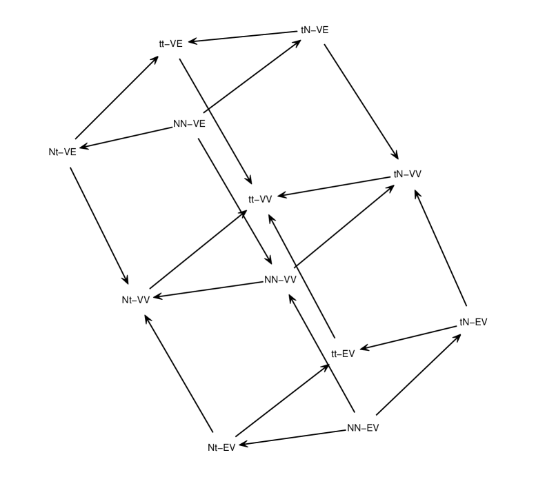
Figure 1: Relationships among the models in the hierarchical initialization strategy. Arrows are oriented from the model used for initialization to the model to be estimated.

Thus, $\widehat{z}_{ng}^{\text{$NN$-VE}}$ is used to initialize the EM of both $tN$-VE and $Nt$-VE, obtaining $\widehat{z}_{ng}^{\text{$tN$-VE}}$ and $\widehat{z}_{ng}^{\text{$Nt$-VE}}$, respectively, while $\widehat{z}_{ng}^{\text{$NN$-EV}}$ is used to initialize the EM of both $tN$-EV and $Nt$-EV, leading to $\widehat{z}_{ng}^{\text{$tN$-EV}}$ and $\widehat{z}_{ng}^{\text{$Nt$-EV}}$, respectively. Also, following the same principle, the model between $NN$-VE and $NN$-EV leading to the maximum likelihood is used to initialize the EM for $NN$-VV. Without going into further details on this hierarchical procedure, in the last step the model between $Nt$-VV, $tN$-VV, $tt$-VE, and $tt$-EV leading to the maximum likelihood is used to initialize the EM of $tt$-VV.

5.3 Convergence criterion

The Aitken acceleration procedure (Aitken, 1926) is used to estimate the asymptotic maximum of the log-likelihood at each iteration of the EM algorithm. Based on this estimate, a decision can be made regarding whether or not the algorithm has reached convergence; that is, whether or not the log-likelihood is sufficiently close to its estimated asymptotic value. The Aitken acceleration at iteration $k$ is given by

$$a^{\left(k\right)}=\frac{l^{\left(k+1\right)}-l^{\left(k\right)}}{l^{\left(k\right)}-l^{\left(k-1\right)}},$$

where $l^{\left(k+1\right)}$, $l^{\left(k\right)}$, and $l^{\left(k-1\right)}$ are the log-likelihood values from iterations $k+1$, $k$, and $k-1$, respectively. Then, the asymptotic estimate of the log-likelihood at iteration $k+1$ (Böhning et al., 1994) is given by

$$l_{\infty}^{\left(k+1\right)}=l^{\left(k\right)}+\frac{1}{1-a^{\left(k\right)}}\left(l^{\left(k+1\right)}-l^{\left(k\right)}\right).$$

In the analyses in Section 7, we follow McNicholas (2010) and stop our algorithms when $l_{\infty}^{\left(k+1\right)}-l^{\left(k\right)}<\epsilon$, with $\epsilon=0.05$.

6 Model selection and clustering performance

In model-based clustering, model selection criteria are commonly used to choice the best model and to select the number of groups. Among them, we will adopt the Bayesian information criterion (BIC; Schwarz, 1978)

$$\text{BIC}=2l\left({\widehat{\mbox{\boldmath$\psi$}}}\right)-m\ln N,$$

where $\widehat{\mbox{\boldmath$\psi$}}$ is the ML estimate of $\psi$, $l\left({$\widehat{\mbox{\boldmath$\psi$}}$}\right)$ is the maximized observed-data log-likelihood, and $m$ is the overall number of free parameters in the model (see the last three columns in Table 1), and the integrated completed likelihood (ICL; Biernacki et al., 2000) in the formulation given by Andrews & McNicholas (2011)

$$\text{ICL}\approx\text{BIC}+\sum_{n=1}^{N}\sum^{G}_{g=1}\text{MAP}\left(\widehat{\tau}_{ng}\right)\ln\widehat{\tau}_{ng}.$$ (35)

A different ICL definition is used by Baek & McLachlan (2011). The two definitions differ on whether or not it is the MAP of the fuzzy clustering in the first part of the entropy. It is not immediately clear from Biernacki et al. (2000) which definition is correct. We have chosen the formulation in (35) because it appears more widely adopted in literature (see, e.g., McNicholas & Murphy, 2008, 2010; McNicholas & Subedi, 2012).

In order to evaluate the clustering performance in cases in which the true classification is known, the adjusted Rand index (ARI; Hubert & Arabie, 1985), and the misclassification rate will be taken into account. We recall that the ARI has an expected value of 0 and perfect classification would result in a value equal to 1.

7 Applications to real data

This section illustrates some real data applications of the family of linear CWMs defined in Section 3.

7.1 Student data

The first application concerns data coming from a survey of $N=270$ students attending a statistics course at the Department of Economics and Business of the University of Catania in the academic year 2011/2012. The questionnaire included seven items, but the analysis we present below only concerns the following subset of variables:

GENDER $$=\text{gender of the respondent;}$$

HEIGHT $$=\text{height of the respondent, measured in centimeters;}$$

WEIGHT $$=\text{weight of the respondent, measured in kilograms;}$$

HEIGHT.F $$=\text{height of respondent's father, measured in centimeters.}$$

There are $G=2$ groups of respondents with respect to the GENDER variable: $N_{M}=119$ males and $N_{F}=151$ females. The considered data are available at http://www.economia.unict.it/punzo/. In the following, the two groups will be simply referred to as $G_{M}$ and $G_{F}$, respectively. Moreover, we shall focus first on the joint distributions of WEIGHT and HEIGHT, then on HEIGHT and HEIGHT.F. In both scenarios, data will be assumed unlabeled with respect to GENDER. However, the true labels will be useful for evaluating the quality of the obtained clustering.

7.1.1 First scenario: HEIGHT and WEIGHT

Figure 2 concerns the observed labeled data. This graphical representation will be simply referred to as the CW-plot.

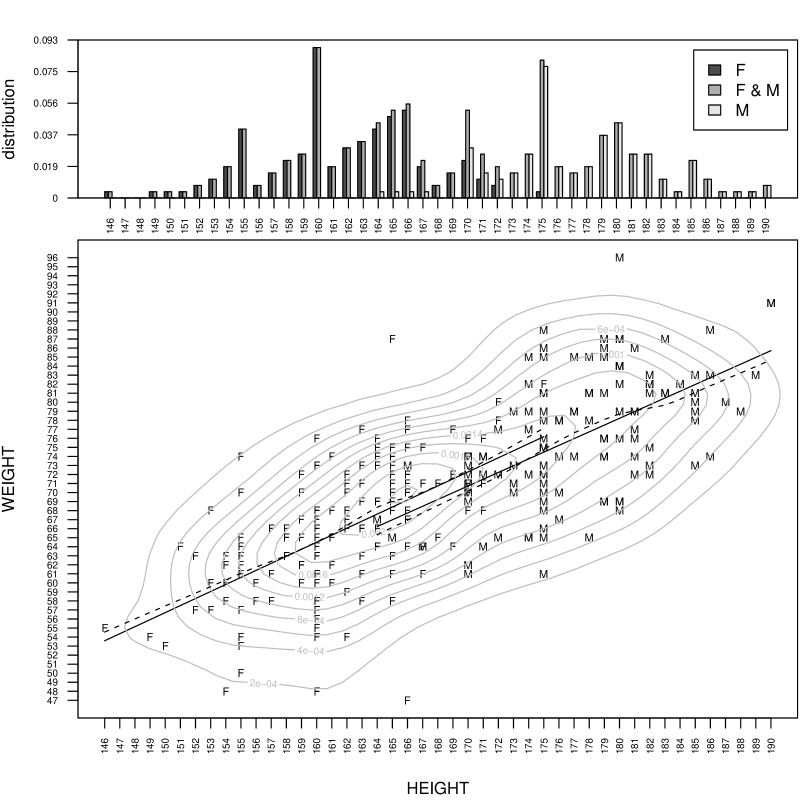
Figure 2: Student Data: CW-plot of HEIGHT and WEIGHT for $119$ male, and $151$ female, students ($\mathsf{M}$ denotes male and $\mathsf{F}$ female).

The top of Figure 2 displays a bar plot of the HEIGHT variable, including the overall empirical marginal density as well as the empirical marginal densities, for $G_{M}$ and $G_{F}$, weighted according to their sizes; bars are color-coded, using a gray scale, with respect to the GENDER variable. We remark that many students tend to approximate their height to ``classical'' values, such as 155, 160, 170, 175, and so on. For classification purposes, the variable HEIGHT separates the two groups quite well. The bottom of Figure 2 is a scatter plot of HEIGHT and WEIGHT, where male and female students are labeled with $\mathsf{M}$ and $\mathsf{F}$, respectively. We give the isodensities of a bivariate normal kernel estimator as computed by the function bkde2D of the R-package KernSmooth (see, e.g., Wand & Jones, 1995). The plot also shows the functional dependence of WEIGHT on HEIGHT separately for $G_{M}$ and $G_{F}$; the solid lines concern the linear regression models while the dashed ones arise from a locally-weighted polynomial regression computed using the lowess function of the R-package stats (see Cleveland, 1979, for details). A simple visual comparison between solid and dashed lines justifies the linearity assumption of WEIGHT on HEIGHT, underlying the linear CWMs of the proposed family. Moreover, the regression lines in Figure 2 seem to indicate that these models have the same parameters in $G_{M}$ and $G_{F}$. In these terms note also that:

1. the $t$-test for equal slopes provides a $p$-value of 0.147,

2. the $t$-test for equal intercepts provides a $p$-value of 0.364, and

3. the F-test of homoscedasticity of residuals in the two groups provides a $p$-value of 0.992.

Now, let us ignore the true classification induced by GENDER and fit the data according to the linear CWMs in Table 1 by using the true value $G=2$. Table 2 lists the values of the BIC, ICL, and ARI for the twelve models.

Table 2: Student Data: Values of the BIC, ICL, and ARI ($G=2$). Bold numbers highlight the best model for each criterion/index.

	VE	EV	VV
$NN$	-3726.197	-3756.561	-3742.947
$tN$	-3737.394	-3762.160	-3754.144
$Nt$	-3731.795	-3766.517	-3749.642
$tt$	-3742.992	-3772.115	-3760.839

(a) BIC

	VE	EV	VV
$NN$	-3750.466	-3880.260	-3767.213
$tN$	-3761.663	-3885.858	-3778.409
$Nt$	-3756.064	-3869.845	-3773.484
$tt$	-3767.261	-3875.443	-3784.681

(b) ICL

	VE	EV	VV
$NN$	0.750	0.008	0.750
$tN$	0.750	0.008	0.750
$Nt$	0.750	0.005	0.776
$tt$	0.750	0.005	0.776

(c) ARI

$NN$-VE (Gaussian marginal and conditional component densities and equal linear model between clusters) is the best model according to both BIC (-3726.197) and ICL (-3750.466). The corresponding CW-plot is displayed in Figure 3. As for the ARI is concerned, in practice we have similar results for all models of type VE and VV.

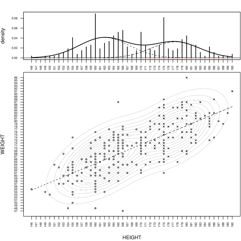
Figure 3: Student Data: CW-plot of HEIGHT and WEIGHT for $NN$-VE ($G=2$).

Thus, the group structure of the data is due to different intra-group distributions for the covariates, while the linear relationship is homogenous. In other words, this is a case of assignment dependence that a standard finite mixture of linear regressions is not able to represent. In order to show it empirically, we have also fitted a mixture of $G=2$ linear Gaussian regressions by means of the flexmix function of the R-package flexmix (Leisch, 2004). The group-conditional distribution of $Y|X$ is Gaussian like in $NN$-VE. Figure 4 highlights that the mixture model with a fixed covariate is not able to recognize the group-structure of the data. This is also confirmed by an ARI value equal to 0.00288.

Figure 4: Student Data: Scatter plot of WEIGHT versus HEIGHT. The two types of lines and symbols displayed arise from the fit of a mixture of $G=2$ Gaussian regressions.

7.1.2 Second scenario: HEIGHT.F and HEIGHT

Figure 5 shows the CW-plot of HEIGHT.F and HEIGHT by considering the classification induced by GENDER.

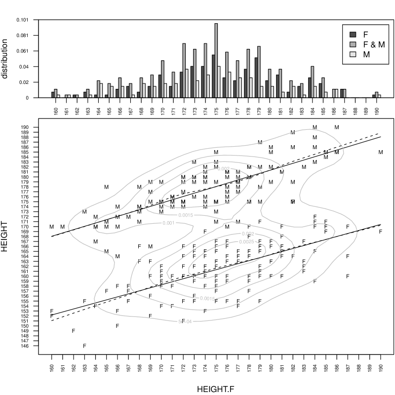
Figure 5: Student Data: CW-plot of HEIGHT and HEIGHT.F for $119$ male and $151$ female, students ($\mathsf{M}$ denotes male and $\mathsf{F}$ female).

Although, also in this case, linearity between variables appear to be reasonable, the linear models for the two groups differ, especially in terms of intercept. Note also that, the $F$-test of homoscedasticity of the residuals in the two groups gives a $p$-value of 0.086 while the $t$-tests for equal slopes and equal intercepts provide practically null $p$-values.

As in Section 7.1.1, we fit the linear CWMs, with $G=2$, ignoring the true classification induced by GENDER. The values of BIC, ICL, and ARI for the twelve models are given in Table 3.

Table 3: Student Data: Values of the BIC, ICL, and ARI ($G=2$). Bold numbers highlight the best model for each criterion/index.

	VE	EV	VV
$NN$	-3726.339	-3594.401	-3601.955
$tN$	-3737.536	-3599.999	-3613.152
$Nt$	-3731.937	-3605.598	-3613.152
$tt$	-3743.134	-3611.196	-3624.348

(a) BIC

	VE	EV	VV
$NN$	-3822.623	-3597.252	-3605.016
$tN$	-3833.820	-3602.850	-3616.212
$Nt$	-3828.221	-3608.449	-3616.212
$tt$	-3839.418	-3614.047	-3627.409

(b) ICL

	VE	EV	VV
$NN$	0.009	0.898	0.912
$tN$	0.009	0.898	0.912
$Nt$	0.009	0.898	0.912
$tt$	0.009	0.898	0.912

(c) ARI

In this case, the best model is $NN$-EV (see also the corresponding CW-plot in Figure 6).

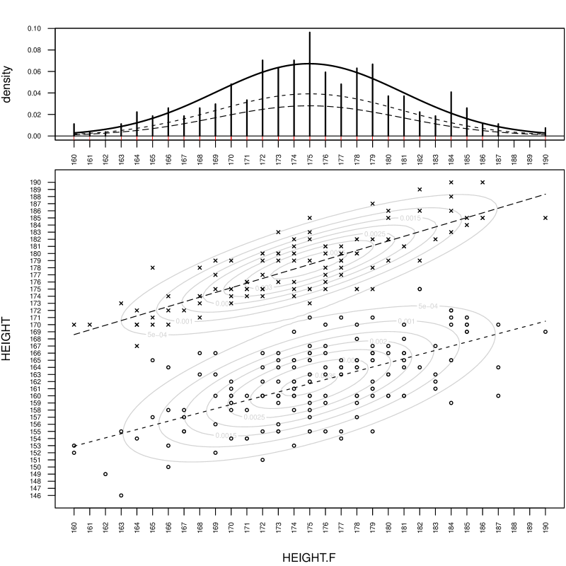
Figure 6: Student Data: CW-plot of HEIGHT.F and HEIGHT for NN-EV ($G=2$).

The fitted model also appears to be a good compromise in terms of the ARI values of Table 4(c). Differently from the first scenario, here the group-structure is due to the different intra-group linear models, while the distribution of the covariate is homogenous. This is an example of assignment independence which can be recognized by a simple mixture of $G=2$ linear (Gaussian) regressions too.

7.2 Tourist data

The second application focuses on $N=180$ monthly data (tourism data) concerning tourist overnights ($X$, data in millions) and attendance at museums and monuments ($Y$, data in millions) in Italy over the 15-year period spanning from January 1996 to December 2010. These data have been recently analyzed by Cellini & Cuccia (2013) and are available at http://www.robertocellini.it/doc/master_specializzazione/Cellini-Cuccia_ApEc2013_data1996-2010.pdf. The CW-plot of the labeled data (with respect to months) is shown in Figure 7.

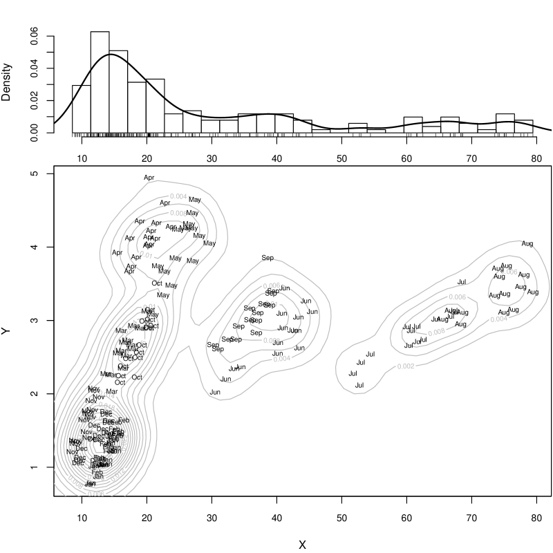
Figure 7: Tourist data: CW-plot of tourist overnights ($X$, in millions) and attendance at museums and monuments ($Y$, in millions) in Italy over the period from January 1996 to December 2010 ($N=180$). The univariate normal kernel density of $X$ is superimposed on the histogram. The isodensities from a bivariate normal kernel density estimator are also visualized on the scatter plot. Month abbreviations are used as labels in the scatter plot.

It is straightforward to note how the heterogeneity of the data reveals a clear group-structure. Figure 8 shows the values of the BIC and the ICL for the models in the proposed family of linear CWMs with $G$ ranging from 1 to 6.

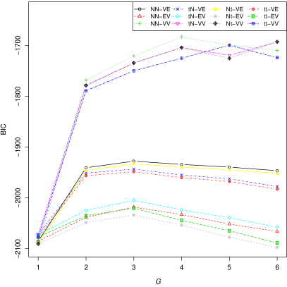
(a) BIC

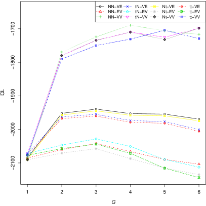
(b) ICL

Figure 8: Tourist data: Values of the BIC and ICL ($G=1,\ldots,6$).

Both criteria (BIC=-1683.727 and ICL=-1689.386) suggest the $NN$-VV, with $G=4$ components, displayed in Figure 9.

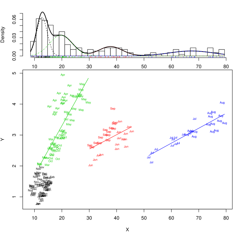
Figure 9: Tourist data: CW-plot of model $NN$-VV with $G=4$ components ($X=$ ``tourist overnights'', in millions, and $Y=$ ``attendance at museums and monuments'', in millions).

Here, it is interesting to analyze the relationship between the obtained clusters – characterized by 4 different slopes – and the time-covariate (months; see Table 4).

group		Jan	Feb	Mar	Apr	May	Jun	Jul	Aug	Sep	Oct	Nov	Dec
1		15	15	0	0	0	0	0	0	0	0	13	15
2		0	0	0	0	0	15	0	0	15	0	0	0
3		0	0	15	15	15	0	0	0	0	15	2	0
4		0	0	0	0	0	0	15	15	0	0	0	0

Table 4: Tourist data: Relation between the $G=4$ clusters, obtained with the fitted $NN$-VV, and the variable time identified by month.

The four clusters, arising from the $NN$-VV, are almost perfectly related to the months (except for two units in November, which concern years 2006 and 2010). In particular, we have:

Group 1

: units from November to February,

Group 2

: units in June and September,

Group 3

: units in March, April, May, and October, and

Group 4

: units in July and August.

This is an example in which the group structure of the data is due to differences both in the intra-group marginal distributions and the linear models.

7.3 Crab data

The third application, based on the very popular crab data set of Campbell & Mahon (1974) on the genus Leptograpsus, has the aim of showing that the $t$-based linear CWMs ($tN$-VE, $tN$-EV, $tN$-VV, $Nt$-VE, $Nt$-EV, $Nt$-VV, $tt$-VE, $tt$-EV, and $tt$-VV) can provide more robust classification than the linear (completely) Gaussian ones ($NN$-VE, $NN$-EV, and $NN$-VV). Attention is focused on the sample of $N=100$ blue crabs, there being $N_{1}=50$ males (group 1) and $N_{2}=50$ females (group 2). Each specimen having $p=2$ measurements (in millimeters): the rear width ($\text{RW}=Y$) and the length along the midline ($\text{CL}=X$) of the carapace.

Following the scheme of McLachlan & Peel (2000, Section 7.8), some outliers were introduced by substituting the original value of $y_{25}$ (11.9) with some atypical values (-15, -10, -5, and 0). This leads to four different ``perturbed'' data sets which are displayed in Figure 10.

(a) $y_{25}=-15$

(b) $y_{25}=-10$

(c) $y_{25}=-5$

(d) $y_{25}=0$

Figure 10: Scatter plots of the sample of $N=100$ blue crabs with different values for $y_{25}$. The variables are rear width (RW) and length along the midline (CL) of the carapace, for $N_{1}=50$ males and $N_{2}=50$ females ($\boldsymbol{\circ}$ denotes male and $\bullet$ female).

Table 5 reports the number of misallocated observations for each of the twelwe models and each perturbed version of the original data set.

		linear Gaussian CWMs (A)				$t$-based linear CWMs (B)
$y_{25}$		$NN$-VE	$NN$-EV	$NN$-VV		$tN$-VE	$tN$-EV	$tN$-VV	$Nt$-VE	$Nt$-EV	$Nt$-VV	$tt$-VE	$tt$-EV	$tt$-VV		$\min\left(A\right)$	$\min\left(B\right)$
-15		40	49	49		40	49	49	40	16	49	40	16	49		40	16
-10		40	49	50		40	49	50	40	16	25	40	16	25		40	16
-5		40	49	50		40	49	50	40	13	24	40	13	24		40	13
0		40	49	50		40	49	50	40	13	21	40	13	21		40	13

Table 5: Crab data: Comparison of the number of misallocated observations when fitting the family of linear CWMs on the sample of $N=100$ blue crabs. Bold numbers highlight the best results for each perturbed data set.

Estimates are obtained by directly using $G=2$. The last two columns report the minimum number of misallocated observations computed over the linear Gaussian CWMs and the $t$-based linear CWMs, respectively. From the bold numbers in Table 5 follows that some of the $t$-based linear CWMs, that is $Nt$-EV and $tt$-EV, are systematically more robust than the linear Gaussian CWMs (see also the results for $Nt$-VV and $tt$-VV). In particular, since the perturbations are inserted ``vertically'' on the $Y$-variable, the best performers have the $t$ distribution for $p\left(y|x,\Omega_{g}\right)$, $g=1,2$.

7.4 f.voles data

The fourth application is based on the f.voles data set described in Flury (1997, Table 5.3.7) and available in the R-package Flury. This is an example with more than one covariate. Data refer to measurements on $N=86$ female voles from two species, M. californicus ($N_{1}=45$) and M. ochrogaster ($N_{2}=45$). Variables used here are: $\mathsf{Species}$ denoting the two species, $\mathsf{Age}$ measured in days, along with other six measurements related to skull (in units of 0.1 mm). The latter are named as in Airoldi & Hoffmann (1984): $\mathsf{L}_{2}=\text{condylo-incisive length}$, $\mathsf{L}_{9}=\text{length of incisive foramen}$, $\mathsf{L}_{7}=\text{alveolar length of upper molar tooth row}$, $\mathsf{B}_{3}=\text{zygomatic width}$, $\mathsf{B}_{4}=\text{interorbital width}$, and $\mathsf{H}_{1}=\text{skull height}$. The scatter plot matrix for grouped-data is shown in Figure 11.

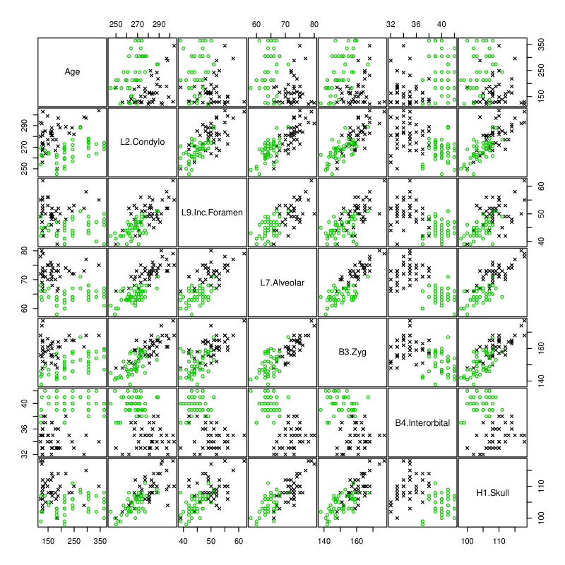
Figure 11: Scatter plot matrix of f.voles data ($\boldsymbol{\circ}$ and $\times$ denote species Microtus ochrogaster and M. californicus, respectively).

The purpose of Airoldi & Hoffmann (1984) was to study age variability in M. californicus and M. ochrogaster and predict age on the basis of the skull measurements. In this study, we assume that data are unlabelled with respect to $\mathsf{Species}$ and compare the classification provided by the three approaches: the family of linear CWMs, mixtures of linear Gaussian regressions (estimated by the R-package flexmix), and parsimonious mixtures of Gaussian distributions (estimated using the R-package mclust; see Fraley et al., 2012, for details). For the first two classes of models, $\mathsf{Age}$ is the response variable $Y$ and the $d=6$ skull measurements are the $\boldsymbol{X}$ variable. For parsimonious mixtures of Gaussian distributions, the vector $\left(Y,\boldsymbol{X}^{\prime}\right)^{\prime}$ is considered as a whole. All the considered models have been fitted with $G=2$.

In the family of linear CWMs, the two models providing the largest values for the BIC and the ICL were $NN$-EV and $NN$-VE (BIC: $NN$-EV = $-3890.397$, $NN$-VE = $-3895.917$; ICL: $NN$-VE = $-3896.143$, $NN$-EV = $-3902.788$). In particular, the two criteria selected a different model, although both the BIC and the ICL yielded quite close values for $NN$-EV and $NN$-VE. On the contrary, the resulting misclassification errors were very different: $NN$-VE (selected by the ICL) yielded a perfect classification, while $NN$-EV (selected by the BIC) yielded a misclassification error of 38.37%. A closer look to the membership probabilities showed that $NN$-VE led to a sharp classification (the entropy term in the ICL resulted 0.23), while the $NN$-EV led to a quite fuzzy classification (the entropy term resulted 12.39). We checked also the AIC for both models, and this agreed with ICL. Thus, $NN$-VE will be the only linear CWM considered hereafter. In the family of parsimonious mixtures of Gaussian distributions, the best model resulted EEE (homoscedastic group-covariance matrices; see Fraley et al., 2012 for details). Thus, we compared the performance of three Gaussian-based models whose classification results are reported in Table 6.

	CWM $NN$-VE	flexmix	mclust model EEE
ARI	1.00000	0.02430	0.90810
misclassification error	0.00000	0.40698	0.02326

Table 6: f.voles data: classification results using different mixture-based approaches ($G=2$).

The finite mixture of Gaussian regressions was the worse approach, reporting a misclassification rate of 0.40698. On the contrary, and surprisingly, our model $NN$-VE attains a perfect classification of the data (we remark the same optimal classification performance was obtained by all the ``-VE'' models in our family).

In conclusion, this is an example of ``strong'' assignment dependence where the group structure only depends by a different distribution of the covariates between the two groups (see also Proposition 1).

8 Comparing the BIC and the ICL

A simulation study is described for comparing the performance of the BIC and the ICL with regard to the proposed family of models. Five scenarios are presented where data are simulated according to the following models: $NN$-EV, $NN$-VE, $NN$-VV, $Nt$-VE, and $tN$-EV. In each scenario, 50 data sets of size $n=400$ are simulated with: $d=1$, $G=2$, and varying parameters. The choice of considering different parameters is made to avoid particular configurations which may favor one of the competitive model selection criteria.

In each replication, the generating (true) model is specified as follows:

• the mixture weight $\pi_{1}$ is randomly generated by a uniform distribution on $\left[0.2,0.8\right]$;

• as the variable $X$ is concerned, we refer to equation (3). Note that, we prefer to leave the matrix notation of the parameters $\mbox{\boldmath$\mu$}_{g}$ and $\mbox{\boldmath$\Sigma$}_{g}$ even if, being $d=1$, they are indeed scalar values. In particular

  • if the model assumes $\mbox{\boldmath$\mu$}_{1}\neq\mbox{\boldmath$\mu$}_{2}$, then $\mbox{\boldmath$\mu$}_{1}$ and $\mbox{\boldmath$\mu$}_{2}$ are randomly generated by a standard normal distribution. If $\mbox{\boldmath$\mu$}_{1}=\mbox{\boldmath$\mu$}_{2}=\mbox{\boldmath$\mu$}$, then $\mu$ is drawn by a standard normal distribution;

  • if the model assumes $\mbox{\boldmath$\Sigma$}_{1}\neq\mbox{\boldmath$\Sigma$}_{2}$, then $\mbox{\boldmath$\Sigma$}_{1}$ and $\mbox{\boldmath$\Sigma$}_{2}$ are randomly generated by a $\chi^{2}_{1}$ distribution. If $\mbox{\boldmath$\Sigma$}_{1}=\mbox{\boldmath$\Sigma$}_{2}=\mbox{\boldmath$\Sigma$}$, then $\Sigma$ is drawn by a $\chi^{2}_{1}$ distribution;

  • if $p\left(\boldsymbol{x}|\Omega_{1}\right)$ and $p\left(\boldsymbol{x}|\Omega_{2}\right)$ are assumed to be $t$;

    • if the model assumes $\nu_{1}\neq\nu_{2}$, then $\nu_{1}$ and $\nu_{2}$ are randomly generated by a uniform distribution on $\left[2,5\right]$;

    • if the model assumes $\nu_{1}=\nu_{2}=\nu$, then $\nu$ is drawn by a uniform distribution on $\left[2,5\right]$;

• as the variable $Y$ is concerned, by referring to equation (2), we have that

  • if the model assumes $\beta_{01}\neq\beta_{02}$ and $\beta_{11}\neq\beta_{12}$, then $\beta_{01}$ and $\beta_{02}$ are randomly generated by a standard normal distribution while $\beta_{11}$ and $\beta_{12}$ are drawn from a uniform distribution on $\left[-2,2\right]$. If $\beta_{01}=\beta_{02}=\beta_{0}$ and $\beta_{11}=\beta_{12}=\beta_{1}$, then $\beta_{0}$ is generated by a standard normal distribution and $\beta_{1}$ is drawn from a uniform distribution on $\left[-2,2\right]$;

  • if the model assumes $\sigma^{2}_{1}\neq\sigma^{2}_{2}$, then $\sigma^{2}_{1}$ and $\sigma^{2}_{2}$ are randomly generated by a $\chi^{2}_{1}$ distribution. If $\sigma^{2}_{1}=\sigma^{2}_{2}=\sigma^{2}$, then $\sigma^{2}$ is generated by a $\chi^{2}_{1}$ distribution;

  • if $p\left(y|\boldsymbol{x},\Omega_{1}\right)$ and $p\left(y|\boldsymbol{x},\Omega_{2}\right)$ are assumed to be $t$

    • if the model assumes $\zeta_{1}\neq\zeta_{2}$, then $\zeta_{1}$ and $\zeta_{2}$ are randomly generated by a uniform distribution on $\left[2,5\right]$;

    • if the model assumes $\zeta_{1}=\zeta_{2}=\zeta$, then $\zeta$ is drawn by a uniform distribution on $\left[2,5\right]$.

The defined models guarantee various degrees of overlap between groups according to the generated parameters.

In each replication, the true model is adopted to generate the data set; thus, all the 12 models are fitted with $G\in\left\{1,2,3\right\}$, leading to a total of 36 fitted models. Table 7 and Table 8 show the results for the BIC and the ICL, respectively. Here, a value in position $\left(i,j\right)$ has to be read as ``number of times that the combination $\left(\text{model},\text{number of groups}\right)$ on column $j$ is selected to fit the true model (with $G=2$) on row $i$''. Bold numbers highlight the number of times that the pair $\left(\text{true model},G=2\right)$ is selected.

	Fitted	$NN$-EV				$NN$-VE				$NN$-VV				$Nt$-EV				$Nt$-VE				$Nt$-VV				$tN$-EV				$tN$-VE				$tN$-VV
True	$G$	1	2	3		1	2	3		1	2	3		1	2	3		1	2	3		1	2	3		1	2	3		1	2	3		1	2	3
$NN$-EV		8	40	0		8	0	0		8	0	0		2	0	0		2	0	0		2	0	0		0	0	0		0	0	0		0	0	0
$NN$-VE		5	0	0		5	40	0		5	0	0		4	0	0		4	0	0		4	0	0		0	0	0		0	1	0		0	0	0
$NN$-VV		0	0	0		0	0	0		0	50	0		0	0	0		0	0	0		0	0	0		0	0	0		0	0	0		0	0	0
$Nt$-VE		0	1	0		0	0	0		0	0	0		5	0	0		5	43	1		5	0	0		0	0	0		0	0	0		0	0	0
$tN$-EV		0	0	0		0	1	0		0	0	0		0	0	0		0	0	0		0	0	0		2	47	0		2	0	0		2	0	0

Table 7: Simulation results for the BIC. Values in the table show the number of times, over 50 replications, that the model, and number of groups, on the column are selected to fit the true model (with two groups) which appears in the corresponding row. Bold numbers highlight the largest number of times that the model selection criteria selects the true model.

	Fitted	$NN$-EV				$NN$-VE				$NN$-VV				$Nt$-EV				$Nt$-VE				$Nt$-VV				$tN$-EV				$tN$-VE				$tN$-VV
True	$G$	1	2	3		1	2	3		1	2	3		1	2	3		1	2	3		1	2	3		1	2	3		1	2	3		1	2	3
$NN$-EV		14	27	0		14	0	0		14	0	0		9	0	0		9	0	0		9	0	0		0	0	0		0	0	0		0	0	0
$NN$-VE		13	0	0		13	24	0		13	0	0		0	0	0		0	0	0		0	0	0		12	0	0		12	1	0		12	0	0
$NN$-VV		0	0	0		0	0	0		0	47	0		1	0	0		1	0	0		1	0	0		2	0	0		2	0	0		2	0	0
$Nt$-VE		0	0	0		0	0	0		0	0	0		15	0	0		15	30	1		15	0	0		2	2	0		2	0	0		2	0	0
$tN$-EV		0	0	0		0	0	0		0	1	0		0	0	0		0	0	0		0	0	0		16	33	0		16	0	0		16	0	0

Table 8: Simulation results for the ICL. Values in the table show the number of times, over 50 replications, that the model, and number of groups, on the column are selected to fit the true model (with two groups) which appears in the corresponding row. Bold numbers highlight the number of times that the model selection criteria selects the true model.

Note that: the columns referred to models of type ``$tt$-'' are missing simply because they have never been selected, and the sum by row is greater than 50 because, when $G=1$ is selected, there is not difference between ``-VV'', ``-VE'', and ``-EV'' (see Section 3). By comparing the results in these tables, the BIC seems to perform better than the ICL. In particular, the ICL selects models with only one group a larger number of times than the BIC. This is probably induced by the scheme of definition of the true model that allows for groups with a strong overlap; thus, the entropy term of the ICL carries out a strong penalization which leads to the choice $G=1$. Figure 12 and Figure 13 display two examples where this happens. From these examples we understand as it is difficult to establish the best model selection criterion; indeed, the ICL may be seen as better if the user actually does not want to separate two mixture components that are so similar that they do not constitute two different clusters in terms of interpretation. So, in general, it depends on the meaning of the data which criterion is better.

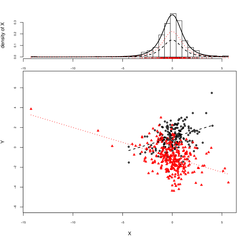
Figure 12: CW-plot of data randomly generated from a $tN$-EV model with $G=2$.

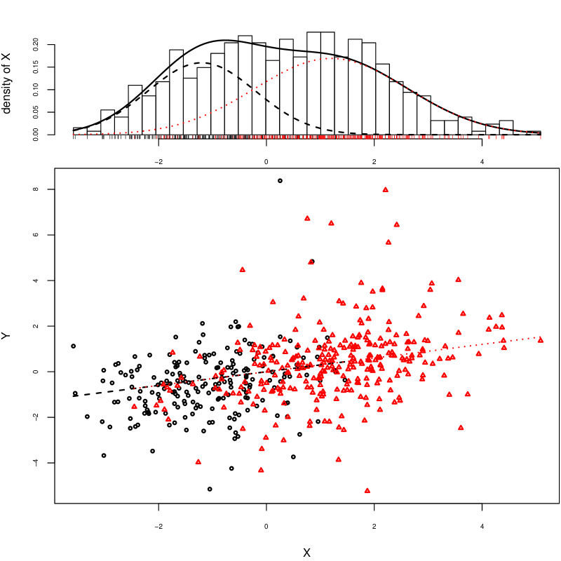
Figure 13: CW-plot of data randomly generated from a $Nt$-VE model with $G=2$.

9 Conclusions and discussion

In this paper, a novel family of twelve linear cluster-weighted models was presented. Such a family represents a flexible and powerful tool for model-based clustering. Maximum likelihood parameter estimation was performed according to the EM algorithm and model selection was accomplished using both the BIC and ICL. Many computational aspects were illustrated and a simple, but very effective, hierarchical random initialization method was introduced. Model-based clustering, using the proposed family, was appreciated on the grounds of some applications to real data. Here, it is interesting to note how the data set related to the survey of students in Section 7.1 justifies and motivates the search for a model in the proposed family.

Future work will involve the extension of the proposed family to the model-based classification context. Moreover, the identifiability issue needs to be adequately addressed; a reference point is given by Hennig (2000). Finally, Section 8 presented first results to find out a suitable model selection criterion and motivates further research in this direction.

Appendix A EM-constraints for parsimonious models

In the following we describe how to impose constraints on the EM algorithm, described in Section 4 for the most general model $tt$-VV, to obtain parameter estimates for all the other models in Table 1. To this end, the itemization given at the beginning of Section 3 will be considered as a benchmark scheme.

A.1 Common $t$ for the component marginal densities

When we constrain all the groups to have a common $t$ distribution for $\boldsymbol{X}$, we have $\mbox{\boldmath$\mu$}_{1}=\cdots=\mbox{\boldmath$\mu$}_{G}=\mbox{\boldmath$\mu$}$, $\mbox{\boldmath$\Sigma$}_{1}=\cdots=\mbox{\boldmath$\Sigma$}_{G}=\mbox{\boldmath$\Sigma$}$, and $\nu_{1}=\cdots=\nu_{G}=\nu$. Thus, in the $\left(k+1\right)$th iteration of the EM algorithm, equations (16) and (18) must be replaced by

$$u_{n}^{\left(k\right)}=\frac{\nu^{\left(k\right)}+d}{\nu^{\left(k\right)}+\delta\left(\boldsymbol{x}_{n},\mbox{\boldmath$\mu$}^{\left(k\right)};\mbox{\boldmath$\Sigma$}^{\left(k\right)}\right)}$$ (36)

and

$$\widetilde{u}_{n}^{\left(k\right)}=\ln u_{n}^{\left(k\right)}+\psi\left(\frac{\nu^{\left(k\right)}+d}{2}\right)-\ln\left(\frac{\nu^{\left(k\right)}+d}{2}\right),$$

respectively. Furthermore, noting that $\sum_{g}\tau_{ng}=1$, equations (23) and (24) can be rewritten as

$$Q_{4}\left(\boldsymbol{\vartheta};\text{{$\boldsymbol{\psi}$}}^{\left(k\right)}\right)=\sum_{n=1}^{N}Q_{4n}\left(\boldsymbol{\vartheta};\text{{$\boldsymbol{\psi}$}}^{\left(k\right)}\right)$$ (37)

and

$$Q_{5}\left(\nu;\text{{$\boldsymbol{\psi}$}}^{\left(k\right)}\right)=\sum_{n=1}^{N}Q_{5n}\left(\nu;\text{{$\boldsymbol{\psi}$}}^{\left(k\right)}\right),$$

respectively, where

$$Q_{4n}\left(\boldsymbol{\vartheta};\text{{$\boldsymbol{\psi}$}}^{\left(k\right)}\right)=\frac{1}{2}\left[-d\ln\left(2\pi\right)+d\widetilde{u}_{n}^{\left(k\right)}-\ln\left|\mbox{\boldmath$\Sigma$}\right|-u_{n}\delta\left(\boldsymbol{x}_{n},\mbox{\boldmath$\mu$};\mbox{\boldmath$\Sigma$}\right)\right]$$

and

$$Q_{5n}\left(\nu;\text{{$\boldsymbol{\psi}$}}^{\left(k\right)}\right)=-\ln\Gamma\left(\frac{\nu}{2}\right)+\frac{\nu}{2}\ln\frac{\nu}{2}+\frac{\nu}{2}\left[\widetilde{u}_{n}^{\left(k\right)}-\ln u_{n}^{\left(k\right)}+\sum_{n=1}^{N}\left(\ln u_{n}^{\left(k\right)}-u_{n}^{\left(k\right)}\right)\right].$$

Maximization of (37), with respect to $\boldsymbol{\vartheta}$, leads to

$$\mbox{\boldmath$\mu$}^{\left(k+1\right)}=\displaystyle\sum_{n=1}^{N}u_{n}^{\left(k\right)}\boldsymbol{x}_{n}\Big{/}\displaystyle\sum_{n=1}^{N}u_{n}^{\left(k\right)}$$

and

$$\mbox{\boldmath$\Sigma$}^{\left(k+1\right)}=\displaystyle\sum_{n=1}^{N}u_{n}^{\left(k\right)}\left(\boldsymbol{x}_{n}-\mbox{\boldmath$\mu$}^{\left(k+1\right)}\right)\left(\boldsymbol{x}_{n}-\mbox{\boldmath$\mu$}^{\left(k+1\right)}\right)^{\prime}\Big{/}\displaystyle\sum_{n=1}^{N}u_{n}^{\left(k\right)}.$$

For the updating of $\nu$, we need to numerically solve the equation

$$\sum_{n=1}^{N}\frac{\partial}{\partial\nu}Q_{5n}\left(\nu;\text{{$\boldsymbol{\psi}$}}^{\left(k\right)}\right)=0,$$

which corresponds to finding $\nu^{\left(k+1\right)}$ as the solution of

$$-\psi\left(\displaystyle\frac{\nu}{2}\right)+\ln\displaystyle\frac{\nu}{2}+1+\displaystyle\displaystyle\sum_{n=1}^{N}\left(\ln u_{n}^{\left(k\right)}-u_{n}^{\left(k\right)}\right)+\psi\left(\displaystyle\frac{\nu^{\left(k\right)}+d}{2}\right)-\ln\left(\displaystyle\frac{\nu^{\left(k\right)}+d}{2}\right)=0.$$ (38)

A.2 Common $t$ for the component conditional densities

Similarly, when we constrain all the groups to have a common $t$ distribution for $Y|\boldsymbol{x}$, we have $\mbox{\boldmath$\beta$}_{11}=\cdots=\mbox{\boldmath$\beta$}_{1G}=\mbox{\boldmath$\beta$}_{1}$, $\beta_{01}=\cdots=\beta_{0G}=\beta_{0}$, $\sigma^{2}_{1}=\cdots=\sigma^{2}_{G}=\sigma^{2}$, and $\zeta_{1}=\cdots=\zeta_{G}=\zeta$. Thus, in the $\left(k+1\right)$th iteration of the EM algorithm, equations (15) and (17) must be replaced by

$$v_{n}^{\left(k\right)}=\frac{\zeta^{\left(k\right)}+1}{\zeta_{g}^{\left(k\right)}+\delta\left[y_{n},\mu\left(\boldsymbol{x}_{n};\mbox{\boldmath$\beta$}^{\left(k\right)}\right);\sigma^{2\left(r\right)}\right]}$$ (39)

and

$$\widetilde{v}_{n}^{\left(k\right)}=\ln v_{n}^{\left(k\right)}+\psi\left(\frac{\zeta^{\left(k\right)}+1}{2}\right)-\ln\left(\frac{\zeta^{\left(k\right)}+1}{2}\right),$$

respectively. Also, equations (21) and (22) can be rewritten as

$$Q_{2}\left(\boldsymbol{\xi};\text{{$\boldsymbol{\psi}$}}^{\left(k\right)}\right)=\sum_{n=1}^{N}Q_{2n}\left(\boldsymbol{\xi};\text{{$\boldsymbol{\psi}$}}^{\left(k\right)}\right)$$ (40)

and

$$Q_{3}\left(\zeta;\text{{$\boldsymbol{\psi}$}}^{\left(k\right)}\right)=\sum_{n=1}^{N}Q_{3n}\left(\zeta;\text{{$\boldsymbol{\psi}$}}^{\left(k\right)}\right),$$

respectively, where

$$Q_{2n}\left(\boldsymbol{\xi};\text{{$\boldsymbol{\psi}$}}^{\left(k\right)}\right)=\frac{1}{2}\left\{-\ln\left(2\pi\right)+\widetilde{v}_{n}^{\left(k\right)}-\ln\sigma^{2}-v_{n}\delta\left[y_{n},\mu\left(\boldsymbol{x}_{n};\mbox{\boldmath$\beta$}\right);\sigma^{2}\right]\right\}$$

and

$$Q_{3n}\left(\zeta;\text{{$\boldsymbol{\psi}$}}^{\left(k\right)}\right)=-\ln\Gamma\left(\frac{\zeta}{2}\right)+\frac{\zeta}{2}\ln\frac{\zeta}{2}+\frac{\zeta}{2}\left[\widetilde{v}_{n}^{\left(k\right)}-\ln v_{n}^{\left(k\right)}+\sum_{n=1}^{N}\left(\ln v_{n}^{\left(k\right)}-v_{n}^{\left(k\right)}\right)\right].$$

Maximization of (40), with respect to $\boldsymbol{\xi}$, leads to the updates

$$\mbox{\boldmath$\beta$}_{1}^{\left(k+1\right)} = \left(\frac{\displaystyle\sum_{n=1}^{N}v_{n}^{\left(k\right)}\boldsymbol{x}_{n}\boldsymbol{x}_{n}^{\prime}}{\displaystyle\sum_{n=1}^{N}v_{n}^{\left(k\right)}}-\frac{\displaystyle\sum_{n=1}^{N}v_{n}^{\left(k\right)}\boldsymbol{x}_{n}}{\displaystyle\sum_{n=1}^{N}v_{n}^{\left(k\right)}}\frac{\displaystyle\sum_{n=1}^{N}v_{n}^{\left(k\right)}\boldsymbol{x}_{n}^{\prime}}{\displaystyle\sum_{n=1}^{N}v_{n}^{\left(k\right)}}\right)^{-1}\cdot$$

$$\cdot\left(\frac{\displaystyle\sum_{n=1}^{N}v_{n}^{\left(k\right)}y_{n}\boldsymbol{x}_{n}}{\displaystyle\sum_{n=1}^{N}v_{n}^{\left(k\right)}}-\frac{\displaystyle\sum_{n=1}^{N}v_{n}^{\left(k\right)}y_{n}}{\displaystyle\sum_{n=1}^{N}v_{n}^{\left(k\right)}}\frac{\displaystyle\sum_{n=1}^{N}v_{n}^{\left(k\right)}\boldsymbol{x}_{n}}{\displaystyle\sum_{n=1}^{N}v_{n}^{\left(k\right)}}\right),$$

$$\beta_{0}^{\left(k+1\right)}=\displaystyle\frac{\displaystyle\sum_{n=1}^{N}v_{n}^{\left(k\right)}y_{n}}{\displaystyle\sum_{n=1}^{N}v_{n}^{\left(k\right)}}-\mbox{\boldmath$\beta$}_{1}^{\left(k+1\right)^{\prime}}\frac{\displaystyle\sum_{n=1}^{N}v_{n}^{\left(k\right)}\boldsymbol{x}_{n}}{\displaystyle\sum_{n=1}^{N}v_{n}^{\left(k\right)}}$$

and

$$\sigma^{2\left(k+1\right)}=\displaystyle\displaystyle\sum_{n=1}^{N}v_{n}^{\left(k\right)}\left[y_{n}-\left(\beta_{0}^{\left(k+1\right)}+\boldsymbol{\beta}_{1}^{\left(k+1\right)^{\prime}}\boldsymbol{x}_{n}\right)\right]^{2}\Big{/}\displaystyle\sum_{n=1}^{N}v_{n}^{\left(k\right)}.$$

For the updating of $\zeta$, we need to numerically solve the equation

$$\sum_{n=1}^{N}\frac{\partial}{\partial\nu}Q_{3n}\left(\zeta;\text{{$\boldsymbol{\psi}$}}^{\left(k\right)}\right)=0,$$

which corresponds to finding $\zeta^{\left(k+1\right)}$ as the solution of

$$-\psi\left(\displaystyle\frac{\zeta}{2}\right)+\ln\displaystyle\frac{\zeta}{2}+1+\displaystyle\displaystyle\sum_{n=1}^{N}\left(\ln v_{n}^{\left(k\right)}-v_{n}^{\left(k\right)}\right)+\psi\left(\displaystyle\frac{\zeta^{\left(k\right)}+1}{2}\right)-\ln\left(\displaystyle\frac{\zeta^{\left(k\right)}+1}{2}\right)=0.$$

A.3 Normal component marginal densities

The normal case for the component distributions of $\boldsymbol{X}$ can be obtained, as stated previously, as a limiting case when $\nu_{g}\rightarrow\infty$, $g=1,\ldots,G$. Then, in (16), $u_{ng}^{\left(k\right)}\rightarrow 1$. Substituting this value into (26) and (27), we obtain

$$\mbox{\boldmath$\mu$}_{g}^{\left(k+1\right)}=\displaystyle\sum_{n=1}^{N}\tau_{ng}^{\left(k\right)}\boldsymbol{x}_{n}\Big{/}\displaystyle\sum_{n=1}^{N}\tau_{ng}^{\left(k\right)}$$

and

$$\mbox{\boldmath$\Sigma$}_{g}^{\left(k+1\right)}=\displaystyle\sum_{n=1}^{N}\tau_{ng}^{\left(k\right)}\left(\boldsymbol{x}_{n}-\mbox{\boldmath$\mu$}_{g}^{\left(k+1\right)}\right)\left(\boldsymbol{x}_{n}-\mbox{\boldmath$\mu$}_{g}^{\left(k+1\right)}\right)^{\prime}\Big{/}\displaystyle\sum_{n=1}^{N}\tau_{ng}^{\left(k\right)}.$$

Naturally, in this case, we do not compute the additional $M$-step maximizing $Q_{5}\left(\text{{$\nu$}};\text{{$\boldsymbol{\psi}$}}^{\left(k\right)}\right)$ in (24). Accordingly, for the sub-case $\mbox{\boldmath$\mu$}_{1}=\cdots=\mbox{\boldmath$\mu$}_{G}=\mbox{\boldmath$\mu$}$ and $\mbox{\boldmath$\Sigma$}_{1}=\cdots=\mbox{\boldmath$\Sigma$}_{G}=\mbox{\boldmath$\Sigma$}$, in equation (36) we have $u_{n}^{\left(k\right)}\rightarrow 1$ and the updated estimates of $\mu$ and $\Sigma$ become

$$\mbox{\boldmath$\mu$}=\displaystyle\frac{1}{n}\sum_{n=1}^{N}\boldsymbol{x}_{n}$$

and

$$\mbox{\boldmath$\Sigma$}=\displaystyle\frac{1}{n}\sum_{n=1}^{N}\left(\boldsymbol{x}_{n}-\mbox{\boldmath$\mu$}\right)\left(\boldsymbol{x}_{n}-\mbox{\boldmath$\mu$}\right)^{\prime},$$

which do not depend on the EM-iterations.

A.4 Normal component conditional densities

The normal case for the component distributions of $Y|\boldsymbol{X}$ can be obtained as a limiting case when $\zeta_{g}\rightarrow\infty$, $g=1,\ldots,G$. Then, in (15), $v_{ng}^{\left(k\right)}\rightarrow 1$. Substituting this value into (28) and (29), we obtain

$$\mbox{\boldmath$\beta$}_{1g}^{\left(k+1\right)} = \left(\frac{\displaystyle\sum_{n=1}^{N}\tau_{ng}^{\left(k\right)}\boldsymbol{x}_{n}\boldsymbol{x}_{n}^{\prime}}{\displaystyle\sum_{n=1}^{N}\tau_{ng}^{\left(k\right)}}-\frac{\displaystyle\sum_{n=1}^{N}\tau_{ng}^{\left(k\right)}\boldsymbol{x}_{n}}{\displaystyle\sum_{n=1}^{N}\tau_{ng}^{\left(k\right)}}\frac{\displaystyle\sum_{n=1}^{N}\tau_{ng}^{\left(k\right)}\boldsymbol{x}_{n}^{\prime}}{\displaystyle\sum_{n=1}^{N}\tau_{ng}^{\left(k\right)}}\right)^{-1}\cdot$$

$$\cdot\left(\frac{\displaystyle\sum_{n=1}^{N}\tau_{ng}^{\left(k\right)}y_{n}\boldsymbol{x}_{n}}{\displaystyle\sum_{n=1}^{N}\tau_{ng}^{\left(k\right)}}-\frac{\displaystyle\sum_{n=1}^{N}\tau_{ng}^{\left(k\right)}y_{n}}{\displaystyle\sum_{n=1}^{N}\tau_{ng}^{\left(k\right)}}\frac{\displaystyle\sum_{n=1}^{N}\tau_{ng}^{\left(k\right)}\boldsymbol{x}_{n}}{\displaystyle\sum_{n=1}^{N}\tau_{ng}^{\left(k\right)}}\right),$$

$$\beta_{0g}^{\left(k+1\right)}=\displaystyle\frac{\displaystyle\sum_{n=1}^{N}\tau_{ng}^{\left(k\right)}y_{n}}{\displaystyle\sum_{n=1}^{N}\tau_{ng}^{\left(k\right)}}-\mbox{\boldmath$\beta$}_{1g}^{\left(k+1\right)^{\prime}}\frac{\displaystyle\sum_{n=1}^{N}\tau_{ng}^{\left(k\right)}\boldsymbol{x}_{n}}{\displaystyle\sum_{n=1}^{N}\tau_{ng}^{\left(k\right)}}$$

and

$$\sigma^{2\left(k+1\right)}_{g}=\displaystyle\displaystyle\sum_{n=1}^{N}\tau_{ng}^{\left(k\right)}\left[y_{n}-\left(\beta_{0g}^{\left(k+1\right)}+\boldsymbol{\beta}_{1g}^{\left(k+1\right)^{\prime}}\boldsymbol{x}_{n}\right)\right]^{2}\Big{/}\displaystyle\sum_{n=1}^{N}\tau_{ng}^{\left(k\right)}.$$

We again do not compute the additional $M$-step maximizing $Q_{3}\left(\text{{$\zeta$}};\text{{$\boldsymbol{\psi}$}}^{\left(k\right)}\right)$ in (22). Accordingly, for the sub-case $\mbox{\boldmath$\beta$}_{11}=\cdots=\mbox{\boldmath$\beta$}_{1G}=\mbox{\boldmath$\beta$}_{1}$, $\beta_{01}=\cdots=\beta_{0G}=\beta_{0}$, and $\sigma^{2}_{1}=\cdots=\sigma^{2}_{G}=\sigma^{2}$, in equation (39) we have $v_{n}^{\left(k\right)}\rightarrow 1$ and the updated estimates of $\mbox{\boldmath$\beta$}_{1}$, $\beta_{0}$, and $\sigma^{2}$ become

$$\mbox{\boldmath$\beta$}_{1}=\left(\displaystyle\frac{1}{n}\displaystyle\sum_{n=1}^{N}\boldsymbol{x}_{n}\boldsymbol{x}_{n}^{\prime}-\frac{1}{n^{2}}\displaystyle\sum_{n=1}^{N}\boldsymbol{x}_{n}\displaystyle\sum_{n=1}^{N}\boldsymbol{x}_{n}^{\prime}\right)^{-1}\left(\displaystyle\frac{1}{n}\sum_{n=1}^{N}y_{n}\boldsymbol{x}_{n}-\frac{1}{n^{2}}\displaystyle\sum_{n=1}^{N}y_{n}\displaystyle\sum_{n=1}^{N}\boldsymbol{x}_{n}\right),$$

$$\beta_{0}=\displaystyle\frac{1}{n}\displaystyle\sum_{n=1}^{N}y_{n}-\frac{1}{n}\mbox{\boldmath$\beta$}_{1}^{\prime}\displaystyle\sum_{n=1}^{N}\boldsymbol{x}_{n}$$

and

$$\sigma^{2}=\displaystyle\frac{1}{n}\displaystyle\sum_{n=1}^{N}\left[y_{n}-\left(\beta_{0}+\boldsymbol{\beta}_{1}^{\prime}\boldsymbol{x}_{n}\right)\right]^{2},$$

which do not depend on the EM-iterations.

References

- Airoldi & Hoffmann (1984) Airoldi, J. P., & Hoffmann, R. S. (1984). Age variation in voles (Microtus californicus, M. ochrogaster) and its significance for systematic studies. Occasional papers of the Museum of Natural History 111 University of Kansas Lawrence, KS.
- Aitken (1926) Aitken, A. (1926). On Bernoulli's numerical solution of algebraic equations. In Proceedings of the Royal Society of Edinburgh (pp. 289–305). volume 46.
- Andrews & McNicholas (2011) Andrews, J., & McNicholas, P. (2011). Extending mixtures of multivariate -factor analyzers. Statistics and Computing, 21, 361–373.
- Andrews et al. (2011) Andrews, J., McNicholas, P., & Subedi, S. (2011). Model-based classification via mixtures of multivariate -distributions. Computational Statistics and Data Analysis, 55, 520–529.
- Baek & McLachlan (2011) Baek, J., & McLachlan, G. (2011). Mixtures of common t-factor analyzers for clustering high-dimensional microarray data. Bioinformatics, 27, 1269–1276.
- Bagnato & Punzo (2013) Bagnato, L., & Punzo, A. (2013). Finite mixtures of unimodal beta and gamma densities and the -bumps algorithm. Computational Statistics, 28, 1571–1597.
- Biernacki et al. (2000) Biernacki, C., Celeux, G., & Govaert, G. (2000). Assessing a mixture model for clustering with the integrated completed likelihood. IEEE Transactions on Pattern Analysis and Machine Intelligence, 22, 719–725.
- Böhning et al. (1994) Böhning, D., Dietz, E., Schaub, R., Schlattmann, P., & Lindsay, B. (1994). The distribution of the likelihood ratio for mixtures of densities from the one-parameter exponential family. Annals of the Institute of Statistical Mathematics, 46, 373–388.
- Brent (1973) Brent, R. (1973). Algorithms for minimization without derivatives. New Jersey: Prentice Hall.
- Campbell & Mahon (1974) Campbell, N. A., & Mahon, R. J. (1974). A multivariate study of variation in two species of rock crab of genus Leptograpsus. Australian Journal of Zoology, 22, 417–425.
- Cellini & Cuccia (2013) Cellini, R., & Cuccia, T. (2013). Museum and monument attendance and tourism flow: A time series analysis approach. Applied Economics, 45, 3473–3482.
- Chatzis & Varvarigou (2008) Chatzis, S., & Varvarigou, T. (2008). Robust fuzzy clustering using mixtures of Student's- distributions. Pattern Recognition Letters, 29, 1901–1905.
- Cleveland (1979) Cleveland, W. (1979). Robust locally weighted regression and smoothing scatterplots. Journal of the American Statistical Association, 74, 829–836.
- Dempster et al. (1977) Dempster, A., Laird, N., & Rubin, D. (1977). Maximum likelihood from incomplete data via the EM algorithm. Journal of the Royal Statistical Society. Series B (Methodological), 39, 1–38.
- Everitt & Hand (1981) Everitt, B., & Hand, D. J. (1981). Finite mixture distributions. Chapman & Hall.
- Flury (1997) Flury, B. (1997). A first course in multivariate statistics. New York: Springer.
- Fraley & Raftery (1998) Fraley, C., & Raftery, A. E. (1998). How many clusters? Which clustering method? Answers via model-based cluster analysis. Computer Journal, 41, 578–588.
- Fraley et al. (2012) Fraley, C., Raftery, A. E., Murphy, T. B., & Scrucca, L. (2012). mclust Version 4 for R: Normal Mixture Modeling for Model-Based Clustering, Classification, and Density Estimation. Technical report 597 Department of Statistics, University of Washington Seattle, Washington, USA.
- Frühwirth-Schnatter (2006) Frühwirth-Schnatter, S. (2006). Finite mixture and Markov switching models. New York: Springer.
- Gershenfeld (1997) Gershenfeld, N. (1997). Non linear inference and cluster-weighted modeling. Annals of the New York Academy of Sciences, 808, 18–24.
- Greselin & Ingrassia (2010) Greselin, F., & Ingrassia, S. (2010). Constrained monotone EM algorithms for mixtures of multivariate distributions. Statistics and Computing, 20, 9–22.
- Hennig (2000) Hennig, C. (2000). Identifiablity of models for clusterwise linear regression. Journal of Classification, 17, 273–296.
- Hubert & Arabie (1985) Hubert, L., & Arabie, P. (1985). Comparing partitions. Journal of Classification, 2, 193–218.
- Ingrassia et al. (2012) Ingrassia, S., Minotti, S. C., & Vittadini, G. (2012). Local statistical modeling via the cluster-weighted approach with elliptical distributions. Journal of Classification, 29, 363–401.
- Ingrassia et al. (2015) Ingrassia, S., Punzo, A., & Vittadini, G. (2015). The generalized linear mixed cluster-weighted model. Journal of Classification, 32.
- Lange et al. (1989) Lange, K. L., Little, R. J. A., & Taylor, J. M. G. (1989). Robust statistical modeling using the distribution. Journal of the American Statistical Association, 84, 881–896.
- Leisch (2004) Leisch, F. (2004). FlexMix: A general framework for finite mixture models and latent class regression in R. Journal of Statistical Software, 11, 1–18.
- McLachlan & Basford (1988) McLachlan, G. J., & Basford, K. E. (1988). Mixture Models: Inference and Applications to Clustering. New York: Marcel Dekker Inc.
- McLachlan & Peel (2000) McLachlan, G. J., & Peel, D. (2000). Finite Mixture Models. New York: John Wiley & Sons.
- McNicholas (2010) McNicholas, P. (2010). Model-based classification using latent gaussian mixture models. Journal of Statistical Planning and Inference, 140, 1175–1181.
- McNicholas & Murphy (2008) McNicholas, P., & Murphy, T. (2008). Parsimonious gaussian mixture models. Statistics and Computing, 18, 285–296.
- McNicholas & Murphy (2010) McNicholas, P., & Murphy, T. (2010). Model-based clustering of microarray expression data via latent gaussian mixture models. Bioinformatics, 26, 2705–2712.
- McNicholas & Subedi (2012) McNicholas, P., & Subedi, S. (2012). Clustering gene expression time course data using mixtures of multivariate t-distributions. Journal of Statistical Planning and Inference, 142, 1114–1127.
- Peel & McLachlan (2000) Peel, D., & McLachlan, G. (2000). Robust mixture modelling using the t distribution. Statistics and Computing, 10, 339–348.
- Punzo (2014) Punzo, A. (2014). Flexible mixture modeling with the polynomial Gaussian cluster-weighted model. Statistical Modelling, 14, 257–291.
- Punzo & Ingrassia (2015a) Punzo, A., & Ingrassia, S. (2015a). Clustering bivariate mixed-type data via the cluster-weighted model. Computational Statistics, .
- Punzo & Ingrassia (2015b) Punzo, A., & Ingrassia, S. (2015b). Parsimonious generalized linear Gaussian cluster-weighted models. In I. Morlini, T. Minerva, & M. Vichi (Eds.), Advances in Statistical Models for Data Analysis Studies in Classification, Data Analysis and Knowledge Organization. Switzerland: Springer International Publishing. Forthcoming.
- Punzo & McNicholas (2013) Punzo, A., & McNicholas, P. D. (2013). Robust Clustering via Parsimonious Mixtures of Contaminated Gaussian Distributions. arXiv.org e-print 1305.4669 available at: http://arxiv.org/abs/1305.4669.
- Punzo & McNicholas (2014a) Punzo, A., & McNicholas, P. D. (2014a). Robust Clustering in Regression Analysis via the Contaminated Gaussian Cluster-Weighted Model. arXiv.org e-print 1409.6019 available at: http://arxiv.org/abs/1409.6019.
- Punzo & McNicholas (2014b) Punzo, A., & McNicholas, P. D. (2014b). Robust High-Dimensional Modeling with the Contaminated Gaussian Distribution. arXiv.org e-print 1408.2128 available at: http://arxiv.org/abs/1408.2128.
- R Development Core Team (2011) R Development Core Team (2011). R: A Language and Environment for Statistical Computing. R Foundation for Statistical Computing. Vienna, Austria.
- Schwarz (1978) Schwarz, G. (1978). Estimating the dimension of a model. The Annals of Statistics, 6, 461–464.
- Shoham (2002) Shoham, S. (2002). Robust clustering by deterministic agglomeration EM of mixtures of multivariate -distributions. Pattern Recognition, 35, 1127–1142.
- Subedi et al. (2013) Subedi, S., Punzo, A., Ingrassia, S., & McNicholas, P. D. (2013). Clustering and classification via cluster-weighted factor analyzers. Advances in Data Analysis and Classification, 7, 5–40.
- Subedi et al. (2015) Subedi, S., Punzo, A., Ingrassia, S., & McNicholas, P. D. (2015). Cluster-weighted -factor analyzers for robust model-based clustering and dimension reduction. Statistical Methods & Applications, 24.
- Titterington et al. (1985) Titterington, D. M., Smith, A. F. M., & Makov, U. E. (1985). Statistical Analysis of Finite Mixture Distributions. New York: John Wiley & Sons.
- Wand & Jones (1995) Wand, M., & Jones, M. (1995). Kernel smoothing volume 60 of Monographs on Statistics and Applied Probability. London: Chapman & Hall.
- Wedel (2002) Wedel, M. (2002). Concomitant variables in finite mixture models. Statistica Neerlandica, 56, 362–375.
- Zellner (1976) Zellner, A. (1976). Bayesian and non-Bayesian analysis of the regression model with multivariate student- error terms. Journal of the American Statistical Association, 71, 400–405.