Euler - Heisenberg effective action and magnetoelectric effect in multilayer graphene

Abstract

The low energy effective field model for the multilayer graphene (at ABC stacking) is considered. We calculate the effective action in the presence of constant external magnetic field $B$ (normal to the graphene sheet). We also calculate the first two corrections to this effective action caused by the in-plane electric field $E$ at $E/B\ll 1$ and discuss the magnetoelectric effect. In addition, we calculate the imaginary part of the effective action in the presence of constant electric field $E$ and the lowest order correction to it due to the magnetic field ($B/E\ll 1$).

1 Introduction

Physics of graphene demonstrates numerous deep relations with fundamental physics such as relativistic quantum mechanics and quantum field theory [1]. The charge carriers in single-layer graphene are topologically protected gapless fermions, which in the vicinity of the nodes automatically acquire the properties of massless Dirac fermions with relativistic spectrum. This naturally induces Lorentz boosts, e.g., in the problem of graphene in crossed electric and magnetic fields [2, 3]. Bilayer [4] and rhombohedral (ABC-stacking) trilayer [5] graphene demonstrate more exotic non-Lorentz-invariant physics of the topologically protected massless chiral fermions with quadractic and cubic dispersion laws, respectively. Such theories are intensively studied now, in particular, in a context of Hořava quantum gravity with anisotropic scaling [6] (this analogy was recently discussed in Ref. [7]). Quantum electrodynamics of bilayer graphene, which experiences the phenomenon of anisotropic scaling, has been considered in Ref. [7] based on a semiclassical approach. Here we derive the effective action of electromagnetic field in bilayer and multilayer graphene based on exact solution of Schrödinger equation. For the case of purely electric field, this has been done recently in Ref. [8]. We will generalize this consideration to the case of crossed fields. This allows us to discuss the magnetoelectric effect in graphene, that is, a change of magnetization due to electric field and change of dielectric polarization due to magnetic field.

In Hořava-Lifshitz quantum gravity [6], the vacuum state is characterized by anisotropic scaling, i.e. the action for gravity is invariant under transformation ${\bf r}\rightarrow b{\bf r}$, $t\rightarrow b^{z}t$, where integer $z\neq 1$ is the analog of the dynamical critical exponent in the theory of phase transitions. The Hořava-Lifshitz gravity in 3+1 spacetime is asymptotic safe, i.e. does not suffer from the ultraviolet divergences, if $z=3$. It is instructive to extend the investigation of the consequences of the anisotropic scaling to quantum field theories with general $z$. It appears that such theories are relevant for the models of the multilayer graphene. These models have nodes in the fermionic spectrum, which are protected by the integer momentum-space topological invariant $N$ expressed in terms of the Hamiltonian, see e.g. [9] (or more generally in terms of the Green’s function [10]). Close to such a node fermions behave as 2+1 massless Dirac particles with energy spectrum ${\cal E}(p)=\pm vp^{N}$, which obeys the anisotropic scaling with $z=N$. That is why one may expect that the effective action for quantum field theories emerging in such systems contains the terms obeying this scaling law, and we consider here such terms in the effective Euler-Heisenberg action for the quantum electrodynamics of the multilayer graphene.

In the simple model with $J$ ABC-stacked graphene layers considered in Ref. [9], the topological invariant coincides with the number of layers, $N=J$. We keep in mind such model, though our consideration can be easily extended to the more general cases with $N\neq J$. We considered the Euler-Heisenberg effective action $S_{eff}({\bf B},{\bf E})$ in two limiting cases, electric field dominated $B<<E$ and magnetic field dominated $E<<B$. Our results for the effective electromagnetic action with $E<<B$ in the system with number of graphene layers in the range $1\leq J\leq 10$ are accumulated in Table 1. This Table demonstrates some peculiar properties of the action. In particular, the $\sim E^{2}$ correction due to electric field decreases quickly with the increase of the number of layers while the coefficient before the main magnetic term increases. At some special value of $J$ (at $J=4$) the $\sim E^{2}$ correction to the effective action vanishes. There are also some special values of $J$, at which the logarithmically divergent term appears; these are $J=2,6,10$. This situation is very similar to what occurs in the relativistic theories, where the logarithmically divergent terms appear only for some special values of space dimension $D$ (see e.g. [11]). This suggests specific regularities in the behavior of quantum field theories, if they are extended to general values of $D$ and $z$.

Table 1 demonstrates that the linear term in electric field arises in the action. It is related with the degeneracy of the first $J$ Landau levels at $E=0$ (they are all zero modes) [1, KP2008]. It describes the linear Stark effect (similar to that in hydrogen atom, due to degeneracy of the states with different orbital quantum numbers), which reflects the spontaneous (broken symmetry) electric polarization emerging in the system. This term can be presented as a scalar product ${\bf E}\cdot{\bf P}$, where the vector ${\bf P}$ is directed along the spontaneous polarization, which in the presence of electric field is oriented along the field. This term is responsible for the magnetoelectric effect in Eq. (59).

In the electric field dominated regime $B<<E$, our main result is the expression for the imaginary part of the effective action and the corresponding Schwinger pair creation rate given by Eqs. (69) and (70).

The paper is organized as follows. In Section 2 we consider the system in pure magnetic field. In Section 3 the system is considered in the presence of both electric and magnetic fields with $E<<B$. In Section 4 the opposite case $B<<E$ is considered. In Section 5 we end with the conclusions.

2 The system in pure magnetic field

The Euler-Heisenberg effective action $S_{eff}$ (and Lagrangian $L_{eff}$) in the considered effective field theory of multilayer graphene is given by the expression for the partition function of the system in the presence of magnetic field $B$ and electric field $E$:

$$Z(T) = \int d\bar{\psi}d\psi\,{\rm exp}\Bigl{(}i\int_{0}^{T}dtd^{2}x\bar{\psi}[i\partial_{t}-{\cal H}[E,B,t]]\psi\Bigr{)}=e^{iTL_{eff}[E,B]}=e^{iS_{eff}[E,B]}$$ (1)

Here $\psi$ is the fermion field (with hidden spin index $A=1,2$ and the index $a=1,2$ that enumerates the number of $2$ - spinors), $\cal H$ is the one - particle Hamiltonian in the presence of external electric and magnetic fields $E$ and $B$, $T\rightarrow\infty$ is time extent. The boundary conditions relate the values of fields at $t=0$ and $t=T$. Usually, for the solution of stationary problems, the anti - periodic boundary conditions are implied for the fermion systems (see, for example, Refs.[12] or [13]). However, in the case of constant nonzero electric field the system is not stationary. We overcome this difficulty considering the path integral in moving reference frame, where electric field vanishes. In this reference frame the problem becomes stationary, and we apply the anti - periodic boundary conditions for the fermion fields (for the details see Appendix A).

2.1 Schrödinger equation

We start with the case of purely magnetic field. First, let us consider the one-particle problem. Its solution is well known (see Chapter 2 in the book [1] and references therein) but it is convenient to repeat briefly the main results for the case of $J$-layer graphene-like material with arbitrary $J$. Here we consider an ideal system, in which the fermionic spectrum is characterized by the nonlinear touching point ${\cal E}(p)=\pm vp^{J}$ (see Fig. 1 for $J=3$). It roughly corresponds to the case of rhombohedral stacking of graphene layers in approximation, in which only the largest in-plane and out-of-plane hopping parameters are taken into account and the trigonal warping is neglected [1]. The spectrum with nonlinear touching points can be realized also in artificial materials as it is done already for $J=1$ [14, 15]. It can also arise in relativistic quantum field theories where the phenomenon of reentrant violation of Lorentz symmetry takes place: the fundamental Lorentz violation at high energies triggers a reentrant violation of Lorentz invariance below some low-energy scale leading to the non-linear touching point (see, e.g., Sec. 12.4 in the book [16]). The Dirac vacuum of fermions, whose massless branch of spectrum has non-linear touching points ${\cal E}(p)=\pm vp^{J}$, induce the non-analytic terms in quantum electrodynamics, which obey the anisotropic scaling ${\bf r}\rightarrow a{\bf r}$, $t\rightarrow a^{J}t$, i.e. the magnetic and electric fields scale as $B\rightarrow Ba^{-2}$ and $E\rightarrow Ea^{-(J+1)}$. Here we will be mainly interested in these non-analytic terms, while the massive Dirac fields give rise to the conventional analytic terms in the Euler-Heisenberg [17] action of the type $\sim B^{4}/m^{5}$, where $m$ is the mass of Dirac particles on branches with energy gap (see Eq. (46) of [11]).

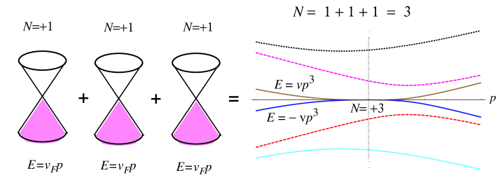
Figure 1: Illustration of branches of spectrum emerging in the system simulating the trilayer graphene with rhombohedral stacking according to Ref. [9]. left: Noninteracting layers. Each layer has its own Dirac fermion with linear spectrum ${\cal E}(p)=\pm v_{F}p$, (on this Figure $v_{F}$ is denoted by $c$, only one conical point at ${\bf p}=0$ is considered in each layer). The conical point is characterized by the momentum-space topological charge $N=1$, so that the total charge of the points at ${\bf p}=0$ is $N=3$ (for Dirac points in the other valley the charge is $N=-3$). right: Interacting layers. The spectrum is shown as function of $p_{x}$ at $p_{y}=0$. Four branches of spectrum correspond to two massive Dirac fermions whose topological charge $N=0$, while two branches with the lowest energy correspond to the massless Dirac particle with nonlinear dispersion ${\cal E}(p)=\pm vp^{3}$, which is characterized by topological charge $N=3$. For the similar stacking of $J$ layers the branch of massless Dirac particles has dispersion ${\cal E}(p)=\pm vp^{J}$, which corresponds to topological charge $N=J$.

We deal with the two-component spinors describing electron states in graphene placed in the external magnetic field $B$ directed along $z$-axis (normal to the graphene plane). We consider the external vector potential in the form: $A_{y}=Bx$ (Landau gauge). The one-particle Hamiltonian in a subsequent parametrization has the form [18, 19, 20]

$$H=v\left(\begin{array}[]{cc}0&\Bigl{(}\hat{p}_{x}-i(\hat{p}_{y}+Bx)\Bigr{)}^{J}\\ \Bigl{(}\hat{p}_{x}+i(\hat{p}_{y}+Bx)\Bigr{)}^{J}&0\end{array}\right)$$ (2)

Here $\hat{p}_{x}=-i\partial_{x}$, $v$ is a constant that is equal to Fermi velocity $v_{F}$ for the case of monolayer, $1/2m$ ($m$ is the effective mass) for the case of bilayer, etc.; we will use the units $\hbar=e=1$. This Hamiltonian describes the lowest energy bands at $\left|\mathcal{E}\right|\ll\left|t_{\bot}\right|$, where $t_{\bot}$ is the interlayer hopping parameter and the energy $\mathcal{E}$ is counted from the band crossing point (neutrality point). Therefore $t_{\bot}\approx 0.4$ eV plays the role of the ultraviolet (UV) cutoff energy (further we denote it by $\Lambda$) for $J>1$; for $J=1$ the Dirac model is applicable till the energies of the order of the in-plane nearest-neighbor hopping parameter $t\approx 3$ eV, which gives us the cutoff energy for this case. The values of $v$ and $\Lambda=t_{\bot}$ are related as $v\approx\Lambda^{1-J}v_{F}^{J}$. From the opposite side of the small energies, the applicability of the model (2) is restricted by trigonal warping effects due to farther interlayer hopping terms; the corresponding energy scale is about 1 to 10 meV [1, 18, 21]. For the case of bilayer, it was shown both experimentally [21] and theoretically (see the recent paper [22] and references therein) that many-body effects can result into a reconstruction of the ground state at these small energies. Since our model is, anyway, inapplicable there we will assume an infrared cutoff (when necessary) of the order of 1 to 10 meV. Many-body effects can also lead to a reconstruction of the ground state for the case of rhombohedral (ABC) trilayer, see, e.g., Ref. [23]. Detailed nature of these instabilities is still unknown and is a subject of intensive debates. We will not take into account the many-body effects in this paper restricting ourselves by the calculations of the effective electromagnetic action in the approximation of noninteracting fermions only.

Stationary Schrödinger equation has the usual form

$$\mathcal{E}\Psi=H\Psi$$ (3)

Later on we imply periodic boundary conditions in space coordinates. That is why $\Psi$ can be decomposed into the sum over the quantized $y$ - momentum: $\Psi(t,x)=\sum\limits_{p_{y}}e^{ip_{y}y-i\mathcal{E}t}\psi_{p_{y},\mathcal{E}}(x)$. $\psi_{p_{y},\mathcal{E}}(x)$ is the eigenfunction of the Hamiltonian ($\mathcal{E}$ is the eigenvalue):

$$v\left(\begin{array}[]{cc}0&\Bigl{(}\hat{p}_{x}-i({p}_{y}+Bx)\Bigr{)}^{J}\\ \Bigl{(}\hat{p}_{x}+i({p}_{y}+Bx)\Bigr{)}^{J}&0\end{array}\right)\psi_{p_{y},\mathcal{E}}(x)=\mathcal{E}\psi_{p_{y},\mathcal{E}}(x)$$ (4)

2.2 Landau levels

Let us now introduce the notations:

$$\epsilon=\frac{\mathcal{E}}{vB^{J/2}},\quad u=\sqrt{B}(x+p_{y}/B)$$ (5)

Then

$$(-i)^{-J}\epsilon{\psi}_{1} = [\partial_{u}+u]^{J}\psi_{2}$$

$$(-i)^{-J}\epsilon{\psi}_{2} = [\partial_{u}-u]^{J}\psi_{1},$$ (6)

where $\psi_{p_{y},\mathcal{E}}=(\psi_{1},\psi_{2})^{T}$. For $\psi_{1,2}$ we have:

$$\psi_{1}=\frac{1}{\epsilon}(-i)^{J}[\partial_{u}+u]^{J}{\psi}_{2}$$

$$\epsilon^{2}{\psi}_{2}=[\partial_{u}-u]^{J}[u+\partial_{u}]^{J}\psi_{2}$$ (7)

As for the oscillator we introduce the annihilation and creation operators $\hat{a}=\frac{1}{\sqrt{2}}[u+\partial_{u}],\hat{a}^{{\dagger}}=\frac{1}{\sqrt{2}}[u-\partial_{u}]$ and $\hat{N}=\hat{a}^{{\dagger}}\hat{a}$. Then

$$\psi_{1}=\frac{2^{J/2}}{\epsilon}(-i)^{J}\hat{a}^{J}{\psi}_{2}$$

$$\epsilon^{2}{\psi}_{2}=2^{J}[\hat{a}^{{\dagger}}]^{J}\hat{a}^{J}\psi_{2}=2^{J}\hat{N}(\hat{N}-1)...(\hat{N}-J+1)\psi_{2}$$ (8)

The normalized solutions are

$$\psi_{1} = \pm\frac{(-i)^{J}}{\sqrt{2}}\frac{B^{1/4}}{2^{n-J}(n-J)!\sqrt{\pi}}e^{-u^{2}/2}H_{n-J}(u)$$

$${\psi}_{2} = \frac{1}{\sqrt{2}}\frac{B^{1/4}}{2^{n}n!\sqrt{\pi}}e^{-u^{2}/2}H_{n}(u)$$ (9)

with integer $n\geq J$ and the eigenvalues $\epsilon=\pm\sqrt{2^{J}n(n-1)...(n-J+1)}$. The solutions for $J>n\geq 0$ have $\psi_{1}=0$ and correspond to $\epsilon=0$:

$$\psi_{1} = 0$$

$${\psi}_{2} = \frac{B^{1/4}}{2^{n}n!\sqrt{\pi}}e^{-u^{2}/2}H_{n}(u)$$ (10)

That is why at each value of $p_{y}$ we have Landau levels with $\mathcal{E}=0$ (the degree of degeneracy is $J$ per flux quantum) and the nondegenerate levels

$$\mathcal{E}=\pm vB^{J/2}\sqrt{2^{J}n(n-1)...(n-J+1)}$$

As usual, we need $-L_{x}/2<p_{y}/B<L_{x}/2,p_{y}=\frac{2\pi}{L_{y}}K_{y},K_{y}\in Z$, where $L_{x,y}$ is the linear size of the graphene sheet in $x,y$ direction.

2.3 Naive expression for the effective action

For pure magnetic field at zero temperature the effective action can be written as follows (for the definition of the effective action $S_{eff}$ and effective Lagrangian $L_{eff}$ and their relation to the spectrum of one - particle excitations see Appendix A)

$$-S_{eff}=-L_{eff}T=-T\sum\,|\mathcal{E}|/2=-g_{s}g_{v}\frac{TL_{x}L_{y}B}{2\pi}v(2B)^{J/2}\sum_{n=J}^{\infty}\sqrt{n(n-1)...(n-J+1)}$$

Here $\sum\,|\mathcal{E}|$ is the sum of the energies over all energy levels; $g_{s}=2$ and $g_{v}=2$ are spin and valley degeneracies, $T$ is the period of the motion. This sum is formally divergent. Using the Hawking trick of the zeta-function regularisation [24] we represent it formally for $J=1$ through the $\zeta$-function:

$$-S_{eff}=-g_{s}g_{v}\frac{TL_{x}L_{y}B}{2\pi}v_{F}(2B)^{1/2}\zeta(-1/2)=g_{s}g_{v}\frac{TL^{2}B}{8\pi^{2}}v_{F}(2B)^{1/2}\zeta(3/2)$$ (11)

where we use the Riemann identity [25, 26]

$$2^{1-s}\Gamma\left(s\right)\zeta\left(s\right)\cos\left(\pi s/2\right)=\pi^{s}\zeta\left(1-s\right)$$ (12)

For $J=1$ the effective action has to be Lorentz invariant. This means that constant magnetic and electric ($E$) fields must enter via the combination $B^{2}-E^{2}/v_{F}^{2}$. Thus, we arrive at the effective action in the presence of both fields:

$$-S_{eff}=\frac{1}{\sqrt{2}}g_{s}g_{v}\frac{TL_{x}L_{y}}{4\pi^{2}}v_{F}[B^{2}-E^{2}/v_{F}^{2}]^{3/4}\zeta(3/2)$$ (13)

This gives us a contribution of vacuum fluctuations (Euler-Heisenberg action [17]) for the single-layer graphene.

From here we get at $B=0$ the imaginary effective action which describes a spontaneous creation of electron-hole pairs from vacuum (Schwinger effect [27, 28, 29, 30, 31, 32, 33, 34]):

$$-2\mathrm{Im}S_{eff}=g_{s}g_{v}\frac{TL_{x}L_{y}}{4v_{F}^{1/2}\pi^{2}}E^{3/2}\zeta(3/2)$$ (14)

This result coincides with that obtained for the vacuum persistence probability using the other methods (see Refs.[30, 7] and references therein).

2.4 Zeta function regularization of the partition function

Let us evaluate the Euler-Heisenberg effective action using the zeta-function regularization [35]. As it is shown in Appendix D this regularization gives the correct values of the Euler-Heisenberg effective action if the divergences are at most logarithmic. In the presence of the divergences that are stronger than logarithmic the zeta - regularized expression for the effective action gives subdominant terms.

To use this regularization we need to calculate the determinant of a positive defined operator. Let us use the valley degeneracy for this purpose. We have

$$\Bigl{(}\mathrm{Det}\,[i\partial_{t}-\mathcal{H}]\Bigr{)}^{2}=\mathrm{Det}\,\Bigl{(}i\partial_{t}-\mathcal{H}\Bigr{)}\Bigl{(}\sigma_{3}[i\partial_{t}-\mathcal{H}]\sigma_{3}\Bigr{)}=\mathrm{Det}\,[i\partial_{t}-\mathcal{H}][i\partial_{t}+\mathcal{H}]=\mathrm{Det}\,[(i\partial_{t})^{2}-\mathcal{H}^{2}]$$ (15)

After the Wick rotation we get

$$\Bigl{(}\mathrm{Det}\,[\partial_{\tau}-\mathcal{H}]\Bigr{)}^{2}=\mathrm{Det}\,\Bigl{(}-[(i\partial_{\tau})^{2}+\mathcal{H}^{2}]\Bigr{)}$$ (16)

Zeta-function regularization [35] then reads:

$$-L_{eff}=-{\cal T}\,\mathrm{Tr}\,\mathrm{log}\,\Bigl{(}[\partial_{\tau}-\mathcal{H}]\Bigr{)}^{g_{s}g_{v}}=\frac{1}{2}g_{s}g_{v}\partial_{s}\Bigl{(}\frac{1}{\Gamma(s)}\,\int_{0}^{\infty}dtt^{s-1}\mathrm{Tr}e^{-[(i\partial_{\tau})^{2}+\mathcal{H}^{2}]t}\Bigr{)}|_{s=0}$$ (17)

Here the system is considered in imaginary time $\tau\in[0,{\cal T}]$, and ${\cal T}=1/T\rightarrow 0$ is the inverse temperature. Below we omit mentioning the exact meaning of $T$ (real or imaginary time). It will always be clear from the context.

It is worth mentioning that the zero modes are to be omitted here. We have:

$$-L_{eff} = \frac{L_{x}L_{y}}{4\pi T}g_{s}g_{v}B\,\partial_{s}\Bigl{(}\frac{1}{\Gamma(s)}\int_{0}^{\infty}dtt^{s-1}\sum_{l,n}\,e^{-[(\frac{2\pi}{T}(l+1/2))^{2}+\mathcal{E}_{n}^{2}]t}\Bigr{)}|_{s=0}$$ (18)

$$= \frac{L_{x}L_{y}}{8\pi\sqrt{\pi}}g_{s}g_{v}B\,\partial_{s}\Bigl{(}\frac{1}{\Gamma(s)}\int_{0}^{\infty}dtt^{s-3/2}\sum_{m,n}\,e^{-\frac{m^{2}T^{2}}{4t}-\mathcal{E}_{n}^{2}t}\Bigr{)}|_{s=0}$$

At zero temperature in the sum over $m$ only the term with $m=0$ survives. Zero modes of $\mathcal{H}$ are omitted and we get:

$$-L_{eff}=\frac{L_{x}L_{y}}{4\pi\sqrt{\pi}}g_{s}g_{v}B\,\partial_{s}\Bigl{(}\frac{1}{\Gamma(s)}\int_{0}^{\infty}dtt^{s-3/2}\sum_{n,\mathcal{E}_{n}>0}\,e^{-\mathcal{E}_{n}^{2}t}\Bigr{)}|_{s=0}$$

The last equation defines analytical function of $s$ at $s>s_{0}$ for some $s_{0}$. This function has to be continued to $s=0$.

Let us check ourselves considering the case $J=1$:

$$-L_{eff} = \frac{L_{x}L_{y}}{4\pi T\sqrt{\pi}}g_{s}g_{v}B\,\partial_{s}\Bigl{(}\frac{1}{\Gamma(s)}\int_{0}^{\infty}dtt^{s-3/2}\sum_{n\geq 1}\,e^{-2v_{F}^{2}Bnt}\Bigr{)}|_{s=0}$$ (19)

$$= \frac{L_{x}L_{y}}{4\pi\sqrt{\pi}}g_{s}g_{v}B\,\partial_{s}\Bigl{(}\frac{1}{\Gamma(s)}\int_{0}^{\infty}dtt^{s-3/2}\,\frac{1}{e^{2v_{F}^{2}Bt}-1}\Bigr{)}|_{s=0}$$

$$= \frac{L_{x}L_{y}}{4\pi\sqrt{\pi}}g_{s}g_{v}B\,\partial_{s}\Bigl{(}\frac{1}{\Gamma(s)}(2v_{F}^{2}B)^{1/2-s}\Gamma(s-1/2)\zeta(s-1/2)\Bigr{)}|_{s=0}$$

$$= \frac{L_{x}L_{y}}{4\sqrt{2}\pi^{2}}g_{s}g_{v}v_{F}B^{3/2}\zeta(3/2)$$

which coincides with the result obtained above.

For arbitrary $J$ we get:

$$-L_{eff} = \frac{L_{x}L_{y}}{4\pi\sqrt{\pi}}g_{s}g_{v}B\,\partial_{s}\Bigl{(}\frac{1}{\Gamma(s)}\int_{0}^{\infty}dtt^{s-3/2}\sum_{n\geq J}\,e^{-v^{2}(2B)^{J}\frac{n!}{(n-J)!}t}\Bigr{)}|_{s=0}$$ (20)

$$= \frac{L_{x}L_{y}}{4\pi\sqrt{\pi}}g_{s}g_{v}B\,\partial_{s}\Bigl{(}\frac{1}{\Gamma(s)}v^{1-2s}(2B)^{J/2-Js}\int_{0}^{\infty}duu^{s-3/2}\,\sum_{n\geq J}\,e^{-\frac{n!}{(n-J)!}u}\Bigr{)}|_{s=0}$$

The resulting expression for the effective action is

$$-L_{eff} = \frac{L_{x}L_{y}}{4\pi\sqrt{\pi}}g_{s}g_{v}2^{J/2}vB^{(J+2)/2}\,\partial_{s}\Bigl{(}\frac{1}{\Gamma(s)}v^{-2s}B^{-Js}\Gamma(s-1/2)f_{J}(s-1/2)\Bigr{)}|_{s=0},$$ (21)

$$f_{J}(s)=\frac{1}{\Gamma(s)}\int_{0}^{\infty}duu^{s-1}\,\sum_{n\geq J}\,e^{-\frac{n!}{(n-J)!}u},\quad s>s_{0}$$

Here the function $f_{J}(s)$ is defined by the given integral for $s>s_{0}=1/J$ while its value at $s=-1/2$ enters the expression for the effective action. The function $f_{J}(s)$ can be considered as the generalization of Riemann zeta-function. For $s>1/J$ it is given by the series:

$$f_{J}(s) = \sum_{n\geq J}\frac{1}{(n)_{-J}^{s}}$$ (22)

$$(n)_{-J}=n(n-1)...(n-J+1)$$

We have ($s\rightarrow 0$):

$$f_{J}(s-1/2) \approx \frac{f_{J}^{(-1)}(-1/2)}{s}+f_{J}^{(0)}(-1/2)$$ (23)

Procedure for the calculation of the values of $f_{J}^{(-1,0)}(-1/2)$ is given in Appendix C. It has been shown that $f_{J}^{(-1)}(-1/2)$ may be nonzero for $J=2(2K+1),K\in Z$.

As a result for the values of $J\neq 2(2K+1)$ we obtain $L_{eff}=L_{x}L_{y}\,l_{eff}$ with

$$-l_{eff} = vB^{(J/2+1)}\,\alpha_{J},$$

$$\alpha_{J} = \Bigl{(}\frac{1}{4\pi\sqrt{\pi}}g_{s}g_{v}2^{J/2}\Gamma(-1/2)f_{J}(-1/2)\Bigr{)},\quad J=1,3,4,5,7,8,9,11,12,13,15,...$$ (24)

Now using the data of Table 2 from Appendix C one can easily calculate values of $\alpha_{J}$.

For $J=2,6,10,14,...$ we have ($\frac{1}{\Gamma(s)}\approx s+\gamma s^{2}$):

$$-l^{(0)}_{eff} = vB^{(J/2+1)}\,\alpha^{(-1)}_{J}\,{\rm log}\Bigl{(}\frac{2v^{2}B^{J}}{\mu^{2}e^{r^{(0)}}}\Bigr{)},$$ (25)

$$r^{(0)}=\gamma+\psi(-1/2)+\frac{f^{(0)}_{J}(-1/2)}{f^{(-1)}_{J}(-1/2)},$$

$$\alpha^{(-1)}_{J}=-\Bigl{(}\frac{1}{4\pi\sqrt{\pi}}g_{s}g_{v}2^{J/2}\Gamma(-1/2)f^{(-1)}_{J}(-1/2)\Bigr{)},$$

Here $\mu$ is a constant of the dimension of mass that is not fixed by the bare theory. It is worth mentioning that $r^{(0)}$ can be absorbed by the dimensional constant $\mu$ via its rescaling: $\tilde{\mu}=\mu e^{r^{(0)}/2}$. Physically, the cutoff at $\mu$ originates from inapplicability of our model at low energies due to trigonal warping and/or many-body effects as was discussed above.

$J$	Effective lagrangian $-l_{eff}/(g_{s}g_{v})$
$1$	$0.04679084006\times v_{F}[B^{2}-E^{2}/v_{F}^{2}]^{3/4}$
$2$	$-0.01989436789\,\times\,vB^{2}\,{\rm log}\Bigl{(}\frac{2v^{2}B^{2}}{\tilde{\mu}^{2}}\Bigr{)}-0.1125395395\times EB^{1/2}-0.03490053651\times\frac{E^{2}}{vB}$
$3$	$0.2431821436\times v_{F}^{2}B^{2}\Lambda^{-1}-0.07113483618\,\times vB^{5/2}-0.1949242002\times EB^{1/2}-0.02123563323\,\times\frac{E^{2}}{vB^{3/2}}$
$4$	$0.2750863237\times v_{F}^{2}B^{2}\Lambda^{-1}+0.1746037024\,\times vB^{3}-0.3462141635\times EB^{1/2}$
$5$	$0.3484677731\times v_{F}^{2}B^{2}\Lambda^{-1}+1.486414997\times vB^{7/2}-0.4740836354\times EB^{1/2}-0.003908473257\,\times\frac{E^{2}}{vB^{5/2}}$
$6$	$0.4434404060\times v_{F}^{2}B^{2}\Lambda^{-1}-0.3133362943\,\times\,vB^{4}\,{\rm log}\Bigl{(}\frac{2v^{2}B^{4}}{\tilde{\mu}^{2}}\Bigr{)}-0.6561212594\times EB^{1/2}-0.001346430685\times\frac{E^{2}}{vB^{3}}$
$7$	$0.5560282734\times v_{F}^{2}B^{2}\Lambda^{-1}+7.837230303\frac{B^{4}}{\Lambda^{5}}v_{F}^{6}-3.222245513vB^{9/2}-0.8183430244EB^{1/2}-0.0004176771170\frac{E^{2}}{vB^{7/2}}$
$8$	$0.6849063582\times v_{F}^{2}B^{2}\Lambda^{-1}+7.438809597\frac{B^{4}}{\Lambda^{5}}v_{F}^{6}+27.35355260\times vB^{5}-1.026656793\times EB^{1/2}-0.0001187738012\times\frac{E^{2}}{vB^{4}}$
$9$	$0.8295068879\times v_{F}^{2}B^{2}\Lambda^{-1}+8.754557174\frac{B^{4}}{\Lambda^{5}}v_{F}^{6}+264.3063672vB^{11/2}-1.217484080EB^{1/2}-0.00003135755874\frac{E^{2}}{vB^{9/2}}$
$10$	$0.9895460087v_{F}^{2}B^{2}\Lambda^{-1}+10.93814698\frac{B^{4}}{\Lambda^{5}}v_{F}^{6}-40.34826486{\rm log}(\frac{2v^{2}B^{10}}{\tilde{\mu}^{2}})vB^{6}-1.449119539\,EB^{1/2}-0.775944555\,10^{-5}\frac{E^{2}}{vB^{5}}$

Table 1: Effective lagrangian $-L_{eff}/(L_{x}L_{y}g_{s}g_{v})$. Here $\Lambda$ is the ultraviolet cutoff ($v\approx\Lambda^{1-J}v_{F}^{J}$), while $\tilde{\mu}$ is the cutoff parameter of the regularization scheme. Both $\Lambda$ and $\tilde{\mu}$ depend on microscopic physics and should be considered as fitting parameters.

2.5 Evaluation of the ultraviolet divergent terms

Below we describe how the zeta - regularized effective action appears in a more conventional expression for the fermionic determinant. Namely, we consider

$$-L_{eff} = -\frac{g_{s}g_{v}}{2T}\mathrm{Tr}\,\mathrm{log}\,\Bigl{(}\frac{(i\partial_{\tau})^{2}+\mathcal{H}^{2}}{(i\partial_{\tau})^{2}+\mathcal{H}_{0}^{2}}\Bigr{)}$$ (26)

$$= \frac{1}{2T}g_{s}g_{v}\int_{0}^{\infty}dtt^{s-1}\Bigl{(}\mathrm{Tr}e^{-[(i\partial_{\tau})^{2}+\mathcal{H}^{2}]t}-\mathrm{Tr}e^{-[(i\partial_{\tau})^{2}+\mathcal{H}_{0}^{2}]t}\Bigr{)}|_{s=0}$$

$$= \frac{L_{x}L_{y}}{8\pi\sqrt{\pi}}g_{s}g_{v}\,\int_{0}^{\infty}dtt^{s-3/2}\Bigl{(}2B\,\sum_{n\geq J}\,e^{-v^{2}(2B)^{J}\frac{n!}{(n-J)!}t}+JB-\int_{0}^{\infty}d\tau\,e^{-v^{2}\tau^{J}t}\Bigr{)}|_{s=0}$$

$$= \frac{L_{x}L_{y}}{8\pi\sqrt{\pi}}g_{s}g_{v}\,v(2B)^{1+J/2}\,\Gamma(s-1/2)\,F_{J}(s-1/2)|_{s=0},$$

$$F_{J}(s)=\frac{1}{\Gamma(s)}\int_{0}^{\infty}dtt^{s-1}\Bigl{(}\sum_{n\geq J}\,e^{-\frac{n!}{(n-J)!}t}+J/2-\int_{0}^{\infty}d\tau\,e^{-\tau^{J}t}\Bigr{)}$$

Here ${\cal H}_{0}$ is the Hamiltonian of the system in the absence of external magnetic field. It is worth mentioning that in this expression we do not omit zero modes of the Hamiltonians $\cal H$ and ${\cal H}_{0}$ as these zero modes are to cancel each other.

At $J=1$ Eq. (26) is convergent, and we find numerically using MAPLE package that $F(-1/2)=\zeta(-1/2)$. This means that for the case $J=1$ zeta - regularized effective action appears when the contribution of the free fermions is subtracted. It is worth mentioning that in the resulting zeta - regularized expression the zero modes of $\cal H$ are omitted while in Eq. (26) are not. This means that the zero mode contribution is subtracted automatically when we subtract the contribution of free fermions.

For the cases $J\geq 2$ Eq. (26) contains divergences:

$$-L_{eff} = \frac{L_{x}L_{y}}{8\pi\sqrt{\pi}}g_{s}g_{v}\,v(2B)^{1+J/2}\,\Gamma(s-1/2)\,F_{J}(s-1/2,\delta)|_{s=0},$$ (27)

$$F_{J}(s,\delta)=\frac{1}{\Gamma(s)}\int_{\delta}^{\infty}dtt^{s-1}\Bigl{(}\sum_{n\geq J}\,e^{-\frac{n!}{(n-J)!}t}+J/2-\int_{0}^{\infty}d\tau\,e^{-\tau^{J}t}\Bigr{)}=f_{J}(s)+F_{J}^{div}(s,\delta)$$

Here $\delta=\frac{v^{2}(2B)^{J}}{\Lambda^{2}}$, where $\Lambda$ is the ultraviolet cutoff. The divergent terms $F_{J}^{div}(s,\delta)$ are calculated in Appendix D. It occurs that the zeta regularized effective action at $J\geq 3$ appears as a subdominant term. The values of the effective action for $J=1,...,10$ (together with the corrections due to the small electric field) are presented in Table 1. For $J=2$ the numerical factor in front of the term $\sim vB^{2}\,{\rm log}\,\frac{\tilde{\mu}^{2}}{\Delta^{2}}$ given in Eq. (6), Eq. (8) of [7] is reproduced with the magnetic scale $\Delta=\sqrt{2}vB$, see also Ref. [36]. For $J\geq 3$ we keep only the dominant ultraviolet divergent terms proportional to $B^{2}$ and the finite correction due to the electric field.

The constants in front of the ultraviolet divergent terms at $J\geq 3$ do not have much sense because these terms appear to be of the same order as the terms that come from the large values of energy ($>\Lambda$), where the energy depends on the momentum (in the absence of external fields) as ${\cal E}\sim|p|$. We do not evaluate the latter terms here. According to [1, 19, 20] we have $v=\Lambda^{1-J}\,v_{F}^{J}$. Therefore, the leading terms for $J\geq 3$ are $\sim v_{F}^{2}B^{2}\Lambda^{-1}$. The complete effective action with the subdominant non - analytical terms and the divergent terms is given by Eq. (27) with the values of $f_{J}(s)$ and $F_{J}^{div}(s,\delta)$ is presented in Appendix C and Appendix D.

3 Effective action in the presence of magnetic field and small electric field

3.1 Schrödinger equation

Let us now consider the case when weak in-plane electric field (along the $x$-axis) is added. We consider the external vector potential in the form: $A_{x}=Et+By$. The one-particle Hamiltonian in a subsequent parametrization has the form (cf. Eq.(2))

$$H=v\left(\begin{array}[]{cc}0&\Bigl{(}(\hat{p}_{x}+Et+By)-i\hat{p}_{y}\Bigr{)}^{J}\\ \Bigl{(}(\hat{p}_{x}+Et+By)+i\hat{p}_{y}\Bigr{)}^{J}&0\end{array}\right)$$ (28)

Again, we try the wave function as $\Psi(t,x))=\sum_{p_{x}}e^{ip_{x}y}\psi_{p}(t)$.

3.2 Zero order approximation and Hall conductivity

Similar to subsection 2.2 we change the variables:

$$\lambda=\frac{E}{\sqrt{2}vB^{(J+1)/2}},\quad u=\sqrt{B}(y+\frac{p_{x}+Et}{B})$$ (29)

and denote

$$\hat{a}^{{\dagger}}=\frac{1}{\sqrt{2}}[-\partial_{u}+u],\quad\hat{a}=\frac{1}{\sqrt{2}}[\partial_{u}+u]$$ (30)

Instead of Eq. (6) the Schrödinger equation reads

$$i[\partial_{t}+vB^{J/2}\lambda(\hat{a}-\hat{a}^{+})]{\psi}_{1} = v(2B)^{J/2}[\hat{a}^{+}]^{J}\psi_{2}$$

$$i[\partial_{t}+vB^{J/2}\lambda(\hat{a}-\hat{a}^{+})]{\psi}_{2} = v(2B)^{J/2}[\hat{a}]^{J}\psi_{1}$$ (31)

When $E$ is small, in the zeroth order approximation we have the analogue of Eq. (7):

$$i\partial_{t}{\psi}_{1} = v(2B)^{J/2}[\hat{a}^{{\dagger}}]^{J}\psi_{2}$$

$$i\partial_{t}{\psi}_{2} = v(2B)^{J/2}[\hat{a}]^{J}\psi_{1}$$ (32)

We have the same Landau levels as without electric field. However, the centers of orbits $y_{c}=-[p_{x}+Et]/B$ move now slowly with the velocity $v_{c}=E/B$ along the $y$-axis. This means that the Hall effect takes place, i.e. when electric field along $x$ axis is turned on, the current along $y$-axis appears if some of the energy states are occupied. The conductivity at zero temperature can be calculated as

$$\sigma=\frac{\bf J}{EL_{x}L_{y}}=g_{s}g_{v}\sum_{n}^{\infty}\frac{B}{2\pi E}\frac{E}{B}\theta(\mu-\mathcal{E}_{n})=\frac{g_{s}g_{v}}{2\pi}\Bigl{(}\frac{J}{2}+I(\mu)\Bigr{)}$$

Here $\mu>0$ is the chemical potential. It has been taken into account that the zero energy levels are half-filled at $\mu=0$. The number of nonzero Landau levels with $\mathcal{E}_{n}<\mu$ is denoted by $I(\mu)$. We come to the well-known conclusion (see Ref.[1]) that at $\mu=+0$ the Hall conductivity is equal to

$$\sigma_{+0} = g_{s}g_{v}\frac{J}{4\pi}$$ (33)

3.3 The first order correction

In the next approximation we take into account the second term in the l.h.s. of Eq. (31):

$$[\epsilon+i\lambda(\hat{a}-\hat{a}^{{\dagger}})]{\psi}_{1}=2^{J/2}[\hat{a}^{{\dagger}}]^{J}\psi_{2}$$

$$[\epsilon+i\lambda(\hat{a}-\hat{a}^{{\dagger}})]{\psi}_{2}=2^{J/2}[\hat{a}]^{J}\psi_{1}$$ (34)

or

$$\epsilon\psi=\left(\begin{array}[]{cc}i\lambda(\hat{a}^{{\dagger}}-\hat{a})&2^{J/2}[\hat{a}^{{\dagger}}]^{J}\\ 2^{J/2}[\hat{a}]^{J}&i\lambda(\hat{a}^{{\dagger}}-\hat{a})\end{array}\right)\psi$$

Here ${\cal E}=vB^{J/2}\epsilon$ is the one - particle energy in the reference frame moving with the velocity $E/B$. In zero order approximation its value is given in subsection 2.2.

One can easily see that the first-order term in expansion of $\epsilon$ in powers of $\lambda$ vanishes for $n\geq J$. For $n\leq J-1$ there is the first order correction to the energy for $J\geq 2$. This correction is given by the eigenvalues $\chi^{(J)}_{k}\lambda$ of the $J\times J$ matrix $i\lambda\Omega$ with

$$\Omega=\left(\begin{array}[]{ccccc}0&1&0&...&...\\ -1&0&\sqrt{2}&..&...\\ 0&...&...&...&...\\ 0&...&-\sqrt{J-2}&0&\sqrt{J-1}\\ 0&...&0&-\sqrt{J-1}&0\end{array}\right)$$ (35)

In particular, we have:

$$\chi^{(2)}=\pm 1;$$

$$\chi^{(3)}=0,\pm\sqrt{3}$$

$$\chi^{(4)}=\pm 2.334414217,\pm 0.7419637843$$

$$\chi^{(5)}=0,\pm 2.856970013,\pm 1.355626179$$

$$\chi^{(6)}=\pm 3.324257431,\pm 0.6167065895,\pm 1.889175877$$

$$\chi^{(7)}=0,\pm 3.750439718,\pm 1.154405395,\pm 2.366759409$$

$$\chi^{(8)}=\pm 4.144547191,\pm 0.5390798102,\pm 1.636519041,\pm 2.802485863$$

$$\chi^{(9)}=0,\pm 4.512745858,\pm 1.023255666,\pm 2.076847980,\pm 3.205429001$$

$$\chi^{(10)}=\pm 4.859462833,\pm 3.581823478,\pm 0.4849357082,\pm 1.465989092,\pm 2.484325840$$ (36)

3.4 The second order approximation

One can easily see that the first-order term in expansion of $\epsilon$ in powers of $\lambda$ vanishes for $n\geq J$ and the second-order term

$$\epsilon_{n}=\epsilon_{n}^{(0)}+\lambda^{2}\sum_{k\neq n}\frac{1}{\epsilon_{n}^{(0)}-\epsilon_{k}^{(0)}}|\psi_{n}^{{\dagger}}(\hat{a}^{{\dagger}}-\hat{a})\psi_{k}|^{2}$$ (37)

should be considered. Here we use that at $|n|\geq J$

$$\psi_{n}=\frac{1}{\sqrt{2}}\left(\begin{array}[]{c}\frac{B^{1/4}}{2^{|n|}|n|!\sqrt{\pi}}e^{-u^{2}/2}H_{|n|}(u)\\ \mathrm{sign}(n)\,\frac{B^{1/4}}{2^{|n|-J}(|n|-J)!\sqrt{\pi}}e^{-u^{2}/2}H_{|n|-J}(u)\end{array}\right)$$ (38)

whereas at $|n|<J$

$$\psi_{n}=\left(\begin{array}[]{c}\frac{B^{1/4}}{2^{|n|}|n|!\sqrt{\pi}}e^{-u^{2}/2}H_{|n|}(u)\\ 0\end{array}\right)$$ (39)

For $n\geq J$ Eq. (37) can be rewritten as

$$\Delta\epsilon_{n} = \epsilon_{n}-\epsilon_{n}^{(0)}=\frac{\lambda^{2}}{4}\Bigl{(}\frac{1}{\epsilon_{n}^{(0)}-\epsilon_{n+1}^{(0)}}[\sqrt{n+1}+\sqrt{n-J+1}]^{2}+\frac{1}{\epsilon_{n}^{(0)}-\epsilon_{n-1}^{(0)}}[\sqrt{n}+\sqrt{n-J}]^{2}$$ (40)

$$+\frac{1}{\epsilon_{n}^{(0)}+\epsilon_{(n+1)}^{(0)}}[\sqrt{n+1}-\sqrt{n-J+1}]^{2}+\frac{1}{\epsilon_{n}^{(0)}+\epsilon_{(n-1)}^{(0)}}[\sqrt{n}-\sqrt{n-J}]^{2}\Bigr{)}=\lambda^{2}\eta_{n},$$

$$\eta_{n}=\frac{(J-4)(2n-(J-1))}{2J(n)_{-J}^{1/2}2^{J/2}}$$

In particular, in the case $J=1$ we have

$$\epsilon_{n}-\epsilon_{n}^{(0)}=-\frac{3\lambda^{2}}{\sqrt{2}}\sqrt{n}$$

For $n<J$ the second order correction vanishes.

In order to make the consideration of the one - particle spectrum complete, we consider in Appendix B the problem in the gauge, where the electric field is introduced via the scalar potential $A_{0}=Ex$. In this gauge there are real energy levels ${\cal E}_{n,p_{y}}={\cal E}_{n}-\frac{E}{B}p_{y}$, where ${\cal E}_{n}$ are calculated above while $p_{y}$ is the momentum along the $y$ axis. The Galilean transformation of energy gives the values of the energy levels equal to ${\cal E}_{n}$ in the reference frame moving along the axis orthogonal to $E$ with the velocity $E/B$.

3.5 Effective lagrangian

In principle, in the presence of external field $E$ the one - particle problem is not stationary, and we do not have usual energy levels in the original reference frame. However, we do have such levels in the frame moving with the velocity $E/B$ along the axis orthogonal to the direction of electric field. In this case the expression for the effective lagrangian is derived in Appendix A. It occurs that this expression coincides with the usual one $\sum\,|{\cal E}|/2$, where the summation is over the energy levels of the system defined in the moving reference frame. This allows us to calculate the effective lagrangian in this case.

For $J=1$ the correction to the effective lagrangian reads:

$$-\Delta L_{eff}=\frac{BL_{x}L_{y}}{2{\pi}}g_{s}g_{v}v_{F}B^{1/2}\sum_{n=1}^{\infty}n^{1/2}\frac{3E^{2}}{2\sqrt{2}v_{F}^{2}B}=\frac{3}{4}\frac{E^{2}}{v_{F}^{2}B^{2}}L_{eff}^{(0)}$$ (41)

where we consider $\sum_{n=1}^{\infty}n^{1/2}$ as $\zeta(-1/2)$.

For $J\geq 2$ the dominant contribution is given by the term linear in $E$ due to the splitting of the lowest Landau Level:

$$-\Delta L^{(1)}_{eff}=-\frac{BL_{x}L_{y}}{2{\pi}}g_{s}g_{v}vB^{J/2}\sum_{n=0}^{J-1}(|\chi^{(J)}_{n}|/2)\frac{E}{\sqrt{2}vB^{(J+1)/2}}=-\frac{L_{x}L_{y}T}{4\sqrt{2}{\pi}}g_{s}g_{v}{E}{B^{1/2}}\sum_{n=0}^{J-1}|\chi_{n}|$$ (42)

For $J\geq 4$ the second order correction can be calculated without use of any regularization:

$$-\Delta L^{(2)}_{eff} = -\frac{BL_{x}L_{y}}{2{\pi}}g_{s}g_{v}vB^{J/2}\sum_{n=J}^{\infty}\eta_{n}\frac{E^{2}}{2v^{2}B^{J+1}}=-\frac{L_{x}L_{y}T}{4{\pi}}g_{s}g_{v}\frac{E^{2}}{vB^{J/2}}\sum_{n=J}^{\infty}\frac{(J-4)(2n-(J-1))}{2J(n)_{-J}^{1/2}2^{J/2}}$$ (43)

$$= -\frac{L_{x}L_{y}}{4{\pi}}g_{s}g_{v}\frac{E^{2}}{vB^{J/2}}\frac{(J-4)(2g_{J}(-1/2)-(J-1)f_{J}(1/2))}{2J2^{J/2}}$$

Here in addition to the function $f_{J}$ given by Eq. (22) we use the function $g_{J}$. These functions are the generalizations of the Riemann zeta-function and are given by:

$$f_{J}(s) = \sum_{n\geq J}\frac{1}{(n)_{-J}^{s}},\quad g_{J}(s)=\sum_{n\geq J}\frac{n}{(n)_{-J}^{s+1}},$$ (44)

$$(n)_{-J}=n(n-1)...(n-J+1)$$

For $J=4$ the correction in Eq. (43) vanishes. For $J>4$ expressions of Eq. (44) are convergent.

In order to calculate the second order correction to the effective action at $J=1,2,3$ we need to apply a certain regularization. First, let us consider the zeta - regularized expression. It can be calculated as follows:

$$-\Delta L^{(2)}_{eff} = \frac{L_{x}L_{y}}{4\pi\sqrt{\pi}}g_{s}g_{v}B\,\partial_{s}\Bigl{(}\frac{1}{\Gamma(s)}\int_{0}^{\infty}dtt^{s-3/2}\sum_{n\geq J}\,[e^{-[\Delta\mathcal{E}+v(2B)^{J/2}\sqrt{\frac{n!}{(n-J)!}}]^{2}t}-e^{-[v(2B)^{J/2}\sqrt{\frac{n!}{(n-J)!}}]^{2}t}]\Bigr{)}|_{s=0}$$ (45)

$$= -\frac{L_{x}L_{y}}{4\pi\sqrt{\pi}}g_{s}g_{v}B\,\partial_{s}\Bigl{(}\frac{1}{\Gamma(s)}v^{1-2s}(2B)^{J/2-Js}\int_{0}^{\infty}duu^{s-3/2}\,\sum_{n\geq J}\,e^{-\frac{n!}{(n-J)!}u}u\frac{E^{2}}{v^{2}B^{J+1}}\eta_{n}\sqrt{\frac{(n)_{-J}}{2^{J}}}\Bigr{)}|_{s=0}$$

$$= -\frac{L_{x}L_{y}}{4\pi\sqrt{\pi}}g_{s}g_{v}B\,\partial_{s}\Bigl{(}\frac{1}{\Gamma(s)}v^{1-2s}(2B)^{J/2-Js}$$

$$\int_{0}^{\infty}duu^{s-3/2}\,\sum_{n\geq J}\,e^{-\frac{n!}{(n-J)!}u}u\frac{E^{2}}{v^{2}B^{J+1}}\frac{2n(J-4)+(5J-J^{2}-4)}{2^{J+1}J}\Bigr{)}|_{s=0}$$

This is the generalization of Eq. (20) to the case of nonzero electric field. The sum over $n$ is convergent due to the exponential factor. Coefficients $\eta_{n}$ are defined in Eq. (85). We obtain ($L_{eff}=L_{x}L_{y}\,l_{eff}$):

$$-l^{(0)}_{eff} = vB^{(J/2+1)}\,\partial_{s}\Bigl{(}\frac{1}{\Gamma(s)}v^{-2s}(2B)^{-Js}\frac{1}{4\pi\sqrt{\pi}}g_{s}g_{v}2^{J/2}\Gamma(s-1/2)f_{J}(s-1/2)\Bigr{)},$$ (46)

$$-\Delta l^{(2)}_{eff} = v^{-1}\frac{E^{2}}{B^{J/2}}\partial_{s}\Bigl{(}\frac{1}{\Gamma(s)}v^{-2s}(2B)^{-Js}\frac{1}{4\pi\sqrt{\pi}}g_{s}g_{v}2^{J/2}\Gamma(s+1/2)$$

$$\Bigl{(}\frac{(J-1)(J-4)}{2^{J+1}J}f_{J}(s+1/2)-\frac{2(J-4)}{2^{J+1}J}g_{J}(s-1/2)\Bigr{)}\Bigr{)}$$

Here the first line reproduces Eq. (21) as it should for the case of vanishing electric field.

Similar to the case of pure magnetic field it is necessary first to calculate $f_{J}(s)$ and $g_{J}(s)$ for the values of $s$, where these series are convergent. Finally we must continue analytically the obtained functions of $s$ to $s=-1/2$. In analogy to the theory of zeta-functions [25, 26], we shall find integral representations for these functions that are convergent at all values of $s$ (see Appendix C). Then the resulting integrals can be evaluated numerically. In addition to representation Eq. (23) we have the similar one for the function $g_{J}$ ($s\rightarrow 0$):

$$f_{J}(s\pm 1/2) \approx \frac{f_{J}^{(-1)}(\pm 1/2)}{s}+f_{J}^{(0)}(\pm 1/2),\quad g_{J}(s\pm 1/2)\approx\frac{g_{J}^{(-1)}(\pm 1/2)}{s}+g_{J}^{(0)}(\pm 1/2)$$ (47)

The calculation of the values of $f_{J}^{(-1,0)}(\pm 1/2),g_{J}^{(-1,0)}(\pm 1/2)$ is described in Appendix C. It has been shown that $f_{J}^{(-1)}(\pm 1/2)$ may be nonzero for $J=2(2K+1),K\in Z$ while $g_{J}^{(-1)}(-1/2)$ may be nonzero for $J=2,4$. We also have $f_{J}^{(-1)}(1/2)=0$ for $J\geq 3$. Remarkably, for $J=2$ the contributions of $f^{(-1)}_{2}(1/2)$ and $g^{(-1)}_{J}(-1/2)$ to the logarithmic term ($\sim\frac{E^{2}}{B}\,{\rm log}B$) cancel each other. Therefore, we have $l_{eff}=l_{eff}^{(0)}+\Delta l_{eff}$ with

$$-\Delta l_{eff} = -\frac{E^{2}}{vB^{J/2}}\gamma^{(0)}_{J},$$ (48)

$$\gamma_{J}=\Bigl{(}\frac{1}{4\pi\sqrt{\pi}}g_{s}g_{v}2^{J/2}\Gamma(-1/2)\Bigl{(}\frac{(J-1)(J-4)}{2^{J+2}J}{f^{(0)}_{J}(1/2)}-\frac{2(J-4)}{2^{J+2}J}[{g^{(0)}_{J}(-1/2)}]\Bigr{)}\Bigr{)},$$

Our results for the effective action at $1\leq J\leq 10$ are accumulated in Table 1. (These results are obtained using the data from Table 2). From this table it follows that the $\sim E^{2}$ correction due to electric field is decreased fast with the increase of the number of layers. At the same time, the coefficient before the main term due to the magnetic field is increased. It is worth mentioning that at $J=4$ the $\sim E^{2}$ correction to the effective action vanishes in this approximation. The linear term in electric field describes the linear Stark effect, which leads to the spontaneous (broken symmetry) electric polarization. This term can be presented as a scalar product ${\bf E}\cdot{\bf P}$, where the vector ${\bf P}$ is directed along the spontaneous polarization, which in the presence of electric field is oriented along the field.

3.6 Conventional regularization

According to our experience due to the consideration of the case when there is the magnetic field only, the ultraviolet divergent terms may be present in the effective action even if its zeta - regularized version is finite. Therefore, let us consider the conventional regularization for the suspicious cases $J=1,2,3$. We subtract the contribution of the fermions at $B=0,E=0$. However, approaching to this limit is performed along the line of constant $\lambda$. This means that the boundary conditions for the fermionic fields in the functional integral for the free fermions are anti - periodic in the reference frame moving with the velocity $V=\lambda v2^{1/2}B^{(J-1)/2}$, ($B\rightarrow 0$) along the axis orthogonal to $E$. (Remind that for the system in the presence of external fields $E$ and $B$ the antiperiodic boundary conditions are adopted in the reference frame moving with the velocity $E/B$.)

$$-L_{eff} = -\frac{g_{s}g_{v}}{2T}\mathrm{Tr}\,\mathrm{log}\,\Bigl{(}\frac{(i\partial_{\tau})^{2}+\mathcal{H}^{2}}{(i\partial_{\tau})^{2}+\mathcal{H}_{0}^{2}}\Bigr{)}$$

$$= \frac{1}{2T}g_{s}g_{v}\int_{0}^{\infty}dtt^{s-1}\Bigl{(}\mathrm{Tr}e^{-[(i\partial_{\tau})^{2}+\mathcal{H}^{2}]t}-\mathrm{Tr}e^{-[(i\partial_{\tau})^{2}+\mathcal{H}_{0}^{2}]t}\Bigr{)}|_{s=0}=L_{eff}^{(0)}+\Delta L_{eff}^{(1)}+$$

$$+\frac{L_{x}L_{y}}{8\pi\sqrt{\pi}}g_{s}g_{v}\,v(2B)^{1+J/2}\,\int_{0}^{\infty}dtt^{s-3/2}\Bigl{(}\sum_{n\geq J}\,{\rm exp}\Bigl{(}-(n)_{-J}t-t\lambda^{2}\frac{(J-4)(2n-(J-1))}{2^{J}J}\Bigr{)}$$

$$-\sum_{n\geq J}\,{\rm exp}\Bigl{(}-(n)_{-J}t\Bigr{)}-\int_{0}^{\infty}d\tau\,{\rm exp}\Bigl{(}-\tau^{J}t-t\lambda^{2}\frac{(J-4)(2\tau-(J-1))}{2^{J}J}\Bigr{)}+\int_{0}^{\infty}d\tau\,{\rm exp}\Bigl{(}-\tau^{J}t\Bigr{)}\Bigr{)}|_{s=0}$$

This is the generalization of Eq. (26) to the case of nonzero $E$. Here ${\cal H}_{0}$ is the Hamiltonian of the system at $B,E\rightarrow 0$ but with the same $\lambda=\frac{E}{v2^{1/2}B^{(J+1)/2}}$ as in $\cal H$.

At $J=1$ Eq. (LABEL:detusualG) is convergent and is equal to the zeta regularized expression. This means that for the case $J=1$ the zeta - regularized effective action appears when the contribution of the fermions with vanishing $B$ and $E$ is subtracted. The limit $E,B\rightarrow 0$ is obtained along the line of constant $\lambda$.

At $J=2$ there is the logarithmic ultraviolet divergence in Eq. (LABEL:detusualG). At $J=3$ Eq. (LABEL:detusualG) contains the divergency but only in $L_{eff}^{(0)}$.

3.7 Magnetoelectic effect

Let us remind (see Appendix A) that

$$-L_{eff}[E,B]={F[E,B]}=-L_{x}L_{y}l_{eff}$$ (50)

where ${F[E,B]}$ is the free energy of the system calculated in the reference frame, where electric field vanishes. It is equal to the effective lagrangian with the minus sign. The quantity

$$\tilde{F}=F+L_{x}L_{y}h(B^{2}-E^{2})/2$$ (51)

(where $h$ is the thickness of the graphene sheet) can be considered as the thermodynamical potential for fixed $E$ and $B$. Actually, $\tilde{F}$ is the effective lagrangian (with the minus sign) for the system of graphene and the constant electromagnetic field. As usual, we may introduce vectors $D$ and $H$:

$$D=P+E,\quad H=B-M,$$ (52)

where $P$ and $M$ are electric and magnetic polarizations (of a unit volume):

$$\frac{dF}{L_{x}L_{y}h}=-PdE-MdB,$$ (53)

Then we have:

$$\frac{1}{L_{x}L_{y}h}d\tilde{F}=-DdE+HdB$$ (54)

Thermodynamical potential $U$ with respect to variables $B$ and $D$ is related to $\tilde{F}$ as follows:

$$U=\tilde{F}+DE$$ (55)

Its differential is

$$\frac{dU}{L_{x}L_{y}h}=EdD+HdB$$ (56)

One can see that this is related to the lagrangian $\tilde{L}_{eff}=-\tilde{F}$ in the same way as the classical Hamiltonian (that is another definition of energy for the electromagnetic field):

$$U=F-E\frac{\partial F}{\partial E}=E\frac{\partial\tilde{L}_{eff}}{\partial E}-\tilde{L}_{eff},\quad\tilde{L}_{eff}=L_{eff}-L_{x}L_{y}h(B^{2}-E^{2})/2$$ (57)

For the case of weak electric field the thermodynamical potential $F$ per unit area depends on $E$ and $B$ as

$$\frac{1}{L_{x}L_{y}}F[E,B]=\frac{1}{L_{x}L_{y}}F[E=0,B]-\omega_{J}B^{1/2}E-\gamma_{J}\frac{E^{2}}{vB^{J/2}}$$ (58)

where the coefficients are given in Table 1.

The magnetization $M=-\frac{1}{L_{x}L_{y}h}\frac{\partial F}{\partial B}$ and electric polarization $P=-\frac{1}{L_{x}L_{y}h}\frac{\partial F}{\partial E}$ of undoped multilayer graphene at zero temperature can be found from this expression. Due to the effect of electric field on Landau levels, the magnetoelectric effect arises, that is, the dependence of magnetization on the electric field and electric polarization on the magnetic field. It is characterized by the quantity

$$h\frac{\partial M}{\partial E}=h\frac{\partial P}{\partial B}=-\frac{1}{L_{x}L_{y}}\frac{\partial^{2}F}{\partial E\partial B}=\Bigl{(}\frac{1}{2}\omega_{J}B^{-1/2}-\gamma_{J}J\frac{E}{vB^{\left(J+2\right)/2}}\Bigr{)}$$ (59)

It follows from Table 1 that the second term in the magnetoelectric effect becomes weaker when the number of layers is increased while the first one is increased with the increase of $J$.

4 The system in the presence of electric field and small magnetic field

4.1 Semiclassics in one-particle Schrödinger equation

To establish the relation with the previous work [7] let us consider the gauge $A_{t}=-Ex,A_{y}=Bx$. Then we have stationary Schrödinger equation $H\Psi=\epsilon\Psi$ with

$$H=\left(\begin{array}[]{cc}Ex&v\Bigl{(}\hat{p}_{x}-i(\hat{p}_{y}+Bx)\Bigr{)}^{J}\\ v\Bigl{(}\hat{p}_{x}+i(\hat{p}_{y}+Bx)\Bigr{)}^{J}&Ex\end{array}\right)$$ (60)

We proceed with the rescaling $z=\Bigl{(}\frac{E}{v}\Bigr{)}^{1/(J+1)}x$, $\omega=\Bigl{(}\frac{1}{vE^{J}}\Bigr{)}^{1/(J+1)}\epsilon$, $\gamma=B\Bigl{(}\frac{v}{E}\Bigr{)}^{2/(J+1)}$, and $\Pi=\Bigl{(}\frac{v}{E}\Bigr{)}^{\frac{1}{J+1}}p_{y}$. Then instead of Eq. (31) we have:

$$(z-\omega)\psi_{1}+(-i\partial_{z}-i(\Pi+\gamma z))^{J}\psi_{2}=0$$

$$(z-\omega)\psi_{2}+(-i\partial_{z}+i(\Pi+\gamma z))^{J}\psi_{1}=0$$ (61)

The first-order semiclassical approximation for $\psi_{1,2}$ gives

$$\psi=e^{\pm i\int(-(\Pi+\gamma z)^{2}+(z-\omega)^{2/J})^{1/2}dz}$$ (62)

We denote here $u=(z-\omega)^{2/J}/\Theta^{2}$ and $\Theta=\Pi+\gamma\omega$. Then

$$\psi=e^{\mp\Theta^{J+1}\frac{J}{2}\int((1+\gamma\Theta^{J-1}u^{J/2})^{2}-u)^{1/2}u^{J/2-1}du}$$ (63)

Integration over the classically forbidden region $(1+\gamma\Theta^{J-1}u^{J/2})^{2}>u$ gives usthe pair production probability. In the limit $\gamma=0$ ($B=0$) we have

$$|\eta_{0}|^{2} = e^{-\alpha_{0}\Theta^{J+1}},$$ (64)

$$\alpha_{0}=2JB\Bigl{(}\frac{3}{2},\frac{J}{2}\Bigr{)}$$

The first-order perturbation in $B$ results in [7]:

$$|\eta|^{2} = e^{-\alpha_{0}\Theta^{J+1}-\gamma^{2}\alpha_{1}\Theta^{3J-1}},$$ (65)

$$\alpha_{1}=3J^{2}B\Bigl{(}\frac{1}{2},\frac{3J}{2}\Bigr{)}$$

4.2 Field-theoretical consideration

The fact that in our approximation the particles do not interact with each other allows to reduce the field-theoretical problem to the quantum-mechanical one. Namely, we arrive at the following pattern. Modes for different values of momenta propagate independently. At $t\leq t_{0}$ all states with negative values of energy are occupied while all states with positive values of energy are vacant. Their evolution in time is governed by the one-particle Schrödinger equation. At $t=t_{0}+T$ the wave function already has the nonzero component corresponding to positive energy. Its squared absolute value is the probability that the electron - hole pair is created. In this section we imply that the gauge is chosen such that $A_{x}=Et,A_{y}=Bx$. However, the probability that the electron-hole pair is created at the definite value of the momentum $p_{y}$ does not depend on the gauge chosen. Therefore we can use here the results of the previous subsection.

Let us calculate the probability that the vacuum remains vacuum $P_{v}$ (vacuum persistence probability). According to the above presented calculation this probability is

$$P_{v}=\prod\limits_{p_{x},p_{y}}\Bigl{(}1-|\eta_{+}|^{2}\Bigr{)}^{g_{s}g_{v}}=e^{-2\mathrm{Im}S}$$ (66)

Here $S$ is the effective action, the factors $g_{s}=2$ and $g_{v}=2$ are spin and valley degeneracies. The product is over the momenta that satisfy

$$ET/2>p_{x}>-ET/2$$ (67)

The total probability of the pair creation per unit area per unit time is

$$\omega = \frac{2\,\mathrm{Im}S}{TL_{x}L_{y}}=-g_{s}g_{v}\frac{E}{2\pi L_{x}}\sum_{p_{y}=\frac{2\pi}{L_{y}}K}\mathrm{log}(1-|\eta_{+}|^{2})$$ (68)

$$\approx -g_{s}g_{v}\frac{E}{2\pi}\int\frac{dp_{y}}{2\pi}\mathrm{log}(1-|\eta_{+}|^{2})$$

$$= g_{s}g_{v}\frac{E^{\frac{J+2}{J+1}}}{2\pi}\Bigl{(}\frac{1}{v}\Bigr{)}^{\frac{1}{J+1}}\sum_{n}\frac{1}{n}\int\frac{d\Theta}{2\pi}e^{-n\alpha_{0}\Theta^{J+1}-\gamma^{2}\alpha_{1}n\Theta^{3J-1}}$$

The final result reads

$$\omega = g_{s}g_{v}\Bigl{(}\frac{1}{v}\Bigr{)}^{\frac{1}{J+1}}\frac{E^{\frac{J+2}{J+1}}}{2(J+1)\pi^{2}(\alpha_{0})^{1/{(J+1)}}}\zeta\Bigl{(}\frac{J+2}{J+1}\Bigr{)}\Gamma\Bigl{(}\frac{1}{J+1}\Bigr{)}$$ (69)

$$\Bigl{(}1-B^{2}\Bigl{(}\frac{v}{E}\Bigr{)}^{4/(J+1)}\frac{\alpha_{1}}{\alpha_{0}^{(3J-1)/(J+1)}}\frac{\zeta\Bigl{(}\frac{3J}{J+1}\Bigr{)}\Gamma\Bigl{(}\frac{3J}{J+1}\Bigr{)}}{\zeta\Bigl{(}\frac{J+2}{J+1}\Bigr{)}\Gamma\Bigl{(}\frac{1}{J+1}\Bigr{)}}\Bigr{)},$$

$$\alpha_{0}=2JB\Bigl{(}\frac{3}{2},\frac{J}{2}\Bigr{)},\quad\alpha_{1}=3J^{2}B\Bigl{(}\frac{1}{2},3J/2\Bigr{)}$$

According to Ref. [31] a different quantity is considered as the pair production rate:

$$\Gamma = \langle|\eta_{+}|^{2}\rangle/(L_{x}L_{y}T)$$ (70)

$$= g_{s}g_{v}\Bigl{(}\frac{1}{v}\Bigr{)}^{\frac{1}{J+1}}\frac{E^{\frac{J+2}{J+1}}}{2(J+1)\pi^{2}(\alpha_{0})^{1/{(J+1)}}}\Gamma\Bigl{(}\frac{1}{J+1}\Bigr{)}\Bigl{(}1-B^{2}\Bigl{(}\frac{v}{E}\Bigr{)}^{4/(J+1)}\frac{\alpha_{1}}{\alpha_{0}^{(3J-1)/(J+1)}}\frac{\Gamma\Bigl{(}\frac{3J}{J+1}\Bigr{)}}{\Gamma\Bigl{(}\frac{1}{J+1}\Bigr{)}}\Bigr{)}$$

5 Conclusions

In this paper we calculated for the first time the effective Euler-Heisenberg action for the multilayer graphene at $ABC$ stacking in the presence of external electric and magnetic fields at $E<<B$. In the opposite limit $B<<E$ we calculated only the imaginary part of the effective action. The considered effective field model is a kind of the quantum field theory with the anisotropic scaling ${\bf r}\rightarrow b{\bf r}$, $t\rightarrow b^{J}t$ that is now becoming relevant. The particular anisotropic scaling with $J=3$ has been applied by Hořava for construction of the quantum theory of gravity, which does not suffer from the ultraviolet divergences. Graphene and graphene like materials may serve as the condensed matter realization of the anisotropic scaling with arbitrary $J$. These materials have nodes in the fermionic spectrum, which are characterized by the integer momentum-space topological invariant $N$. Close to such a node fermions behave as 2+1 massless Dirac particles with energy spectrum ${\cal E}(p)=\pm vp^{N}$. These fermions induce the terms in the action for electrodynamic fields, which obey the anisotropic scaling with $J=N$.

Here we considered the fixed space dimension $D=2$, but with point node of arbitrary topological charge $N$. This is somehow orthogonal to the relativistic systems studied in literature, which in case of massless fermions corresponds to the fixed $J=1$, but with arbitrary space dimension $D$. In our case some features (in the presence of the external fields $E<<B$) look similar, but some are new:

1. For $D=2$ and $J=2$ the logarithmic term appears that is naturally expected from the one-loop consideration. In relativistic theories the same logarithmic term naturally appears in one-loop consideration in conventional electrodynamics with massless fermions, which corresponds to $J=1$ and $D=3$.

2. For $J\geq 3$ there are terms that are divergent stronger than logarithmically. These terms depend on magnetic field but do not depend on electric field.

3. At $J\geq 2$ the magnetoelectric effect is dominated by the lowest Landau level. Its degeneracy in the absence of electric field is $J$. In the presence of electric field the degeneracy is eliminated. The corresponding term in the effective action is proportional to $E$, which produces the analog of the Stark effect. The lowest subdominant terms are proportional to $E^{2}$ and are decreased fast with the increase of $J$. There is a specific value $J=4$, at which the quadratic $E^{2}$ term is absent.

4. The term which contains the logarithm $\sim B^{\frac{J+2}{2}}\ln B$ appears only for special values of $J$, such as $J=2,6,10$. This situation is similar to what occurs in relativistic theories, where the existence of the term $\sim B^{\frac{D+1}{2}}\ln B$ depends on the space dimension $D$ [11]. It would be interesting to consider the general case of arbitrary $D$ and $J$.

It is worth mentioning that at $J<3$ the zeta regularization of the effective action at $E<<B$ gives the correct result. At the same time, for $J\geq 3$ the zeta regularization gives only the subdominant terms. The dominant ultraviolet divergent terms are calculated as well. This case is similar to the case of Dirac fermions in the presence of external fields $E<<B$ and with the dimension of space $D>3$.

In the case $E>>B$ we calculate the imaginary part of the effective action with the small correction $\sim B^{2}$.

In future it will be instructive to consider electrodynamics arising in general case of arbitrary space dimension $D$ in the vicinity of the manifold of zeroes in the fermionic energy spectrum of different dimensions. It appears that the point nodes in $D=3$ described by topological charge $N>1$ gives rise to the more complicated structure of the induced electromagnetic action: the QED has different scaling laws for different directions in space. For example, fermions emerging near the Weyl point with topological charge $N=2$ have the $J=1$ scaling law for spectrum along an anisotropy axis and the $J=2$ scaling for the transverse directions (see Sec. 12.4 in Ref. [16]).

Appendix A: Effective action and one-particle spectrum

In expression Eq. (1) for the effective action $\cal H$ is the one - particle hamiltonian in the presence of external electric and magnetic fields $E$ and $B$. This hamiltonian may depend on time explicitly (as, for example, in Eq. (28)). $T\rightarrow\infty$ is time. It is implied that $E$ is small enough, so the electron - hole pairs are not created. Our main supposition here is that there exists the transformation $y\rightarrow\tilde{y}=y+Vt$, with some velocity $V$ such that in new variables $(x,\tilde{y},t)$ we have $[i\partial_{t}-{\cal H}[E,B,t]]\psi(x,y,t)=[i\partial_{t}-\tilde{\cal H}[E,B]]\psi(x,\tilde{y},t)$, where $\tilde{H}$ does not depend on time. For Eq. (28) this is achieved for $V=E/B$.

The system is considered with anti - periodic in time boundary conditions (in this new coordinates): $\psi(t+T,{x},\tilde{y})=-\psi(t,{x},\tilde{y})$. Suppose we find the solution $\zeta$ of the equation $(i\partial_{t}-{\cal H})\zeta=0$ such that $\zeta_{\cal E}(t+T)=e^{-i{\cal E}T}\zeta_{\cal E}$. In this case $\cal E$ is the eigenvalue of $\tilde{\cal H}$ and the analogue of the energy level. Actually, it is the energy level in the case, when $\cal H$ does not depend on time from the very beginning, and $V=0$. Then $\Psi_{k,{\cal E}}=e^{i\frac{\pi}{T}(2k+1)t+i{\cal E}t}\zeta_{\cal E}$ is the eigenfunction of the operator $(i\partial_{t}-{\cal H})$:

$$(i\partial_{t}-{\cal H})\Psi_{k,{\cal E}}=-(\frac{\pi}{T}(2k+1)+{\cal E})\Psi_{k,{\cal E}}$$ (71)

The product over $k$ can be calculated as follows

$$\Pi_{k=-N,...,N}[\frac{\pi}{T}(2k+1)+{\cal E}] = \Bigl{(}\Pi_{k=-N,...,N}\frac{\pi}{T}(2k+1)\Bigr{)}\Bigl{(}\Pi_{k}[1+\frac{{\cal E}T}{\pi(2k+1)}]\Bigr{)}$$ (72)

$$\approx \Bigl{(}\frac{\pi}{2Na}\Bigr{)}^{2N}\Bigl{(}\Pi^{N}_{k=-N+1}(2k+1)\Bigr{)}\,{\rm cos}({\cal E}T/2),$$

where $T=2Na$, and $a$ is the lattice spacing. This results in

$${\rm Det}(i\partial_{t}-{\cal H})=e^{-\Omega_{0}}\Pi_{n}{\rm cos}({\cal E}_{n}T/2),$$ (73)

where $\Omega_{0}$ depends on the details of the regularization but does not depend neither on $T$ nor on the spectrum in continuum limit. The values ${\cal E}_{n}$ depend on the parameters of the hamiltonian, index $n$ enumerates these values.

Partition function receives the form (see also [13, 37]):

$$Z(T) = e^{-\Omega_{0}}\,\sum_{\{K_{n}\}=0,1}\,{\rm exp}\Bigl{(}i\frac{T}{2}\sum_{n}{\cal E}_{n}-iT\sum_{n}K_{n}{\cal E}_{n}\Bigr{)}=e^{-\Omega_{0}}\,\sum_{\{K_{n}\}=0,1}\,{\rm exp}\Bigl{(}-iT\sum_{n}K_{n}{\cal E}_{n}\Bigr{)}$$ (74)

Following [13] we interpret Eq. (74) as follows. $K_{n}$ represents the number of occupied states with the values of ”energy” ${\cal E}_{n}$, $K_{n}$ may be $0,1$. The term $\sum_{n}{\cal E}_{n}$ vanishes because the values ${\cal E}_{n}$ come in pairs with opposite signs.

After the Wick rotation we arrive at

$$Z(-i\tau) = e^{-\Omega_{0}}\,\sum_{\{K_{n}\}=0,1}\,{\rm exp}\Bigl{(}-\tau\sum_{n}K_{n}{\cal E}_{n}\Bigr{)}$$ (75)

Here $\tau=\frac{1}{\cal T}$, where $\cal T$ is temperature. In the formal limit ${\cal T}\rightarrow 0$ only $K_{n}=[1-{\rm sign}{\cal E}_{n}]/2$ survives. Thus we get

$$Z(-i/{\cal T}) = e^{-\Omega_{0}}\,{\rm exp}\Bigl{(}-\frac{1}{\cal T}\sum_{n,{\cal E}_{n}\leq 0}{\cal E}_{n}[E,B]\Bigr{)},\quad{\cal T}\rightarrow 0$$ (76)

Comparing Eq (76) and Eq. (1) we obtain

$$Z({T}) = e^{-\Omega_{0}}\,{\rm exp}\Bigl{(}-iT\sum_{n,{\cal E}_{n}\leq 0}{\cal E}_{n}[E,B]\Bigr{)}$$ (77)

and

$$L_{eff}[E,B]=-\sum_{n,{\cal E}_{n}\leq 0}{\cal E}_{n}[E,B]=+(1/2)\sum_{n,}|{\cal E}_{n}[E,B]|=-F[E,B]$$ (78)

Here $F[E,B]$ is the free energy of the system in the presence of constant external fields $E$ and $B$ in the reference frame moving with the velocity $E/B$ in the direction orthogonal to the direction of $E$. (Actually, in this reference frame the electric field is absent.) $S=TL_{eff}[E,B]$ is the effective action.

Appendix B: Energy levels in the presence of magnetic field and small electric field

5.1 Schrodinger equation

Here we consider the case when weak in-plane electric field (along the $x$-axis) is added. We use here the same gauge as in Sect. 4.1. Namely, the external vector potential has the form: $A_{y}=Bx$ while the scalar potential is $A_{t}=Ex$. The one-particle Hamiltonian has the form of Eq. (60)

$$H=\left(\begin{array}[]{cc}Ex&v\Bigl{(}\hat{p}_{x}-i(\hat{p}_{y}+Bx)\Bigr{)}^{J}\\ v\Bigl{(}\hat{p}_{x}+i(\hat{p}_{y}+Bx)\Bigr{)}^{J}&Ex\end{array}\right)$$ (79)

We try the wave function as $\Psi(t,x))=\sum_{p_{y}}e^{ip_{y}y}\psi_{p}(x,t)$.

5.2 Zero order approximation

Let us change the variables:

$$\tilde{\epsilon}=\frac{\mathcal{E}+\frac{E}{B}p_{y}}{vB^{J/2}},\quad\epsilon=\frac{\mathcal{E}}{vB^{J/2}},\quad\lambda=\frac{E}{\sqrt{2}vB^{(J+1)/2}},\quad u=\sqrt{B}(x+\frac{p_{y}}{B}),\quad u_{c}=-\frac{p_{y}}{B^{1/2}}$$ (80)

and denote

$$\hat{a}^{{\dagger}}=\frac{1}{\sqrt{2}}[-\partial_{u}+u],\quad\hat{a}=\frac{1}{\sqrt{2}}[\partial_{u}+u]$$ (81)

Instead of Eq. (31) the Schrödinger equation reads

$$\tilde{\epsilon}\psi=(\epsilon-\lambda\sqrt{2}u_{c})\psi=\left(\begin{array}[]{cc}\lambda(\hat{a}^{{\dagger}}+\hat{a})&(-i)^{J}2^{J/2}[\hat{a}]^{J}\\ (i)^{J}2^{J/2}[\hat{a}^{{\dagger}}]^{J}&\lambda(\hat{a}^{{\dagger}}+\hat{a})\end{array}\right)\psi$$

When $E$ is small, in the zeroth order approximation over $\lambda$ we have:

$$({\cal E}+\frac{E}{B}p_{y}){\psi}_{1} = v(2B)^{J/2}[\hat{a}^{{\dagger}}]^{J}\psi_{2}$$

$$({\cal E}+\frac{E}{B}p_{y}){\psi}_{2} = v(2B)^{J/2}[\hat{a}]^{J}\psi_{1}$$ (82)

(We cannot neglect here $\frac{E}{B}p_{y}$ because $p_{y}$ may be large.) We have the same Landau levels as without electric field shifted by $\frac{E}{B}p_{y}$.

5.3 The first order correction

In the next approximation we have

$$\tilde{\epsilon}\psi=\left(\begin{array}[]{cc}\lambda(\hat{a}^{{\dagger}}+\hat{a})&(-i)^{J}2^{J/2}[\hat{a}^{{\dagger}}]^{J}\\ i^{J}2^{J/2}[\hat{a}]^{J}&\lambda(\hat{a}^{{\dagger}}+\hat{a})\end{array}\right)\psi$$

One can easily see that the first-order term in expansion of $\epsilon$ in powers of $\lambda$ vanishes for $n\geq J$. For $n\leq J-1$ there is the first order correction to the energy for $J\geq 2$. This correction is given by the eigenvalues $\chi^{(J)}_{k}\lambda$ of the $J\times J$ matrix $\lambda\Omega$ with

$$\Omega=\left(\begin{array}[]{ccccc}0&1&0&...&...\\ 1&0&\sqrt{2}&..&...\\ 0&...&...&...&...\\ 0&...&\sqrt{J-2}&0&\sqrt{J-1}\\ 0&...&0&\sqrt{J-1}&0\end{array}\right)$$ (83)

We have the same eigenvalues as in Eq. (36).

5.4 The second order approximation

One can easily see that the first-order term in expansion of $\epsilon$ in powers of $\lambda$ vanishes for $n\geq J$ and the second-order term

$$\tilde{\epsilon}_{n}=\tilde{\epsilon}_{n}^{(0)}+\lambda^{2}\sum_{k\neq n}\frac{1}{\tilde{\epsilon}_{n}^{(0)}-\tilde{\epsilon}_{k}^{(0)}}|\psi_{n}^{{\dagger}}(\hat{a}^{{\dagger}}+\hat{a})\psi_{k}|^{2}$$ (84)

should be considered. Here we use that the functions $\psi_{n}$ are given by Eq. (9), Eq. (10).

For $n\geq J$ Eq. (84) can be rewritten as

$$\Delta\tilde{\epsilon}_{n} = \lambda^{2}\eta_{n},$$ (85)

$$\eta_{n}=\frac{(J-4)(2n-(J-1))}{2J(n)_{-J}^{1/2}2^{J/2}}$$

For $n<J$ the second order correction vanishes.

Appendix C: Calculation of the functions $f_{J}(s)$ and $g_{J}(s)$.

5.5 Integral representations

In this section we describe regular procedure for the calculation of $f_{J}(s)$ and $g_{J}(s)$.

For $s>1/J$ ($s>2/J$) we have

$$f_{J}(s) = \sum_{n\geq J}\frac{1}{[(n)_{-J}]^{s}},\quad g_{J}(s)=\sum_{n\geq J}\frac{n}{[(n)_{-J}]^{s+1}}$$ (86)

We apply to these sums the Plana summation formula [26], Vol. 1, 1.9(11):

$$\sum_{n=0}^{\infty}f(n) = \frac{1}{2}f(0)+\int^{\infty}_{0}f(\tau)\,d\tau+i\int^{\infty}_{0}\Bigl{(}f(it)-f(-it)\Bigr{)}\frac{dt}{e^{2\pi t}-1}$$ (87)

This formula works if:

1. $f(x)$ is regular for ${\rm Re}\,x\geq 0$,

2. $e^{-2\pi|t|}f(\tau+it)\rightarrow 0$ at $t\rightarrow\infty$, $0\leq\tau<\infty$,

3. $\int e^{-2\pi|t|}|f(\tau+it)|dt\rightarrow 0$ at $\tau\rightarrow\infty$

Therefore, we obtain:

$$f_{J}(s) = \frac{1}{2[J!]^{s}}+\int^{\infty}_{0}(\tau+J)_{-J}^{-s}\,d\tau+i\int^{\infty}_{0}\Bigl{(}(it+J)_{-J}^{-s}-(-it+J)_{-J}^{-s}\Bigr{)}\frac{dt}{e^{2\pi t}-1},\quad s>1/J$$

$$g_{J}(s) = \frac{J}{2[J!]^{s}}+\int^{\infty}_{0}(\tau+J)_{-J}^{-s-1}(\tau+J)\,d\tau$$ (88)

$$+i\int^{\infty}_{0}\Bigl{(}(it+J)_{-J}^{-s-1}(it+1)-(-it+J)_{-J}^{-s-1}(-it+1)\Bigr{)}\frac{dt}{e^{2\pi t}-1},\quad s>2/J$$

Here

$$(\tau+J)_{-J} = \frac{\Gamma(\tau+J+1)}{\Gamma(\tau+1)}=(\tau+J)(\tau+J-1)...(\tau+1)$$ (89)

Now the divergences of the sums over $n$ at $s\leq 1/J$ and $s\leq 2/J$ correspondingly are concentrated within the integrals over $\tau$. At $s>1/J$ ($s>2/J$) we may represent these integrals as follows:

$$I_{J}(s)=\int^{\infty}_{0}(\tau+J)_{-J}^{-s}\,d\tau,\quad\tilde{I}_{J}(s)=\int^{\infty}_{0}(\tau+J)_{-J}^{-s-1}(\tau+J)\,d\tau$$

$$0=\oint_{C}z_{-J}^{-s}dz=I_{J}(s)(1+e^{-i\pi Js})+\int_{-1}^{J}z_{-J}^{-s}dz$$

$$0=\oint_{C}z_{-J}^{-s-1}zdz=\tilde{I}_{J}(s)(1-e^{-i\pi J(s+1)})+(J-1)e^{-i\pi J(s+1)}I_{J}(s+1)+\int_{-1}^{J}z_{-J}^{-s-1}zdz$$ (90)

Here contour $C$ consists of the integral from $-\infty+i0$ to $-1+i0$, the part of the circle that belongs to the upper half - plane, starts at $-1+i0$, and ends at $J+i0$, then the part of the real axis from $J+i0$ to $\infty+i0$. The contour is closed via the half - circle at infinity in the upper half - plane. We obtain:

$$I_{J}(s)=-\frac{1}{1+e^{-i\pi Js}}\oint_{-1}^{J}z_{-J}^{-s}dz$$

$$\tilde{I}_{J}(s)=-\frac{1}{1-e^{-i\pi J(s+1)}}\oint_{-1}^{J}z_{-J}^{-s-1}zdz-\frac{(J-1)e^{-i\pi J(s+1)}}{1-e^{-i\pi J(s+1)}}I_{J}(s+1)$$ (91)

Here integrals $\oint$ are taken along the half - circle $z=\frac{J-1}{2}+\frac{J+1}{2}e^{i\omega},\,\omega\in[0,\pi]$. The given integrals are convergent for all values of $s$, probably, except for $s=(2K+1)/J$ and $s=2Q/J-1$, $K,Q\in Z$.

For the ordinary Riemann zeta function there is the Hermit representation ([26], Vol.1, 1.10, (7)). Using the expressions listed above we derive the analogue of this representation:

$$f_{J}(s) = \frac{1}{2[J!]^{s}}-\frac{1}{1+e^{-i\pi Js}}\oint_{-1}^{J}z_{-J}^{-s}dz+2\int^{\infty}_{0}\frac{{\rm sin}\,s[{\rm arctg}\,\frac{t}{J}+...+{\rm arctg}\,t]}{(t^{2}+J^{2})^{s/2}...(t^{2}+1)^{s/2}}\frac{dt}{e^{2\pi t}-1},$$

$$g_{J}(s) = \frac{J}{2[J!]^{s}}-\frac{1}{1-e^{-i\pi J(s+1)}}\oint_{-1}^{J}z_{-J}^{-s-1}zdz+\frac{J-1}{1-e^{-i\pi J(s+1)}}\frac{e^{-i\pi J(s+1)}}{1+e^{-i\pi J(s+1)}}\oint_{-1}^{J}z_{-J}^{-s-1}dz$$ (92)

$$+2\int^{\infty}_{0}\frac{{\rm sin}(\,(s+1)[{\rm arctg}\,\frac{t}{J}+...+{\rm arctg}\,t]-{\rm arctg}\,\frac{t}{J}])}{(t^{2}+J^{2})^{(s+1)/2}...(t^{2}+1)^{(s+1)/2}}\frac{(t^{2}+J^{2})^{1/2}\,dt}{e^{2\pi t}-1}$$

This expression gives the analytical continuation of the series Eq. (86) to all values of $s$. From this representation we conclude that $f_{J}(s)$ may have a simple pole at $s=(2K+1)/J,K\in Z$ while $g_{J}(s)$ may have poles at $s=(2K+1)/J$ or $s=(2Q+1)/J-1$.

5.6 Particular cases

At $J=1$ expression (92) is the Hermit integral representation for the $\zeta$ - function (see [26], Vol.1, 1.10, (7)).

We have ($s\rightarrow 0$):

$$f_{J}(s\pm 1/2) \approx \frac{f_{J}^{(-1)}(\pm 1/2)}{s}+f_{J}^{(0)}(\pm 1/2),\quad g_{J}(s\pm 1/2)\approx\frac{g_{J}^{(-1)}(\pm 1/2)}{s}+g_{J}^{(0)}(\pm 1/2)$$ (93)

We have verified integral representations Eq. (92) using MAPLE package for several values of $s$ and $J$ such that the series Eq. (86) are convergent. Next, we calculated numerically the values of $f^{(0,-1)}_{J}(\pm 1/2)$ and $g^{(0,-1)}_{J}(-1/2)$ using these integral representations at $J=2,...,10$.

At $J=2$ we come to:

$$f_{2}(s) = \frac{1}{2^{s+1}}+I_{2}(s)+2\int^{\infty}_{0}\frac{{\rm sin}\,s[{\rm arctg}\,\frac{t}{2}+{\rm arctg}\,t]}{(t^{2}+2^{2})^{s/2}(t^{2}+1)^{s/2}}\frac{dt}{e^{2\pi t}-1},$$

$$g_{2}(s) = \frac{1}{2^{s}}+\tilde{I}_{2}(s)+2\int^{\infty}_{0}\frac{{\rm sin}(\,(s+1)[{\rm arctg}\,\frac{t}{2}+{\rm arctg}\,t]-{\rm arctg}\,\frac{t}{2}])}{(t^{2}+2^{2})^{(s+1)/2}(t^{2}+1)^{(s+1)/2}}\frac{(t^{2}+2^{2})^{1/2}\,dt}{e^{2\pi t}-1}$$ (94)

For $J=2$ we may check expression Eq. (91) using integral representation for the hypergeometric function ([26], (2.12), Eq. (5)):

$$I_{2}(s)=\frac{1}{2^{s+1}(s-1/2)}F(s,1,2s,1/2)=\frac{1}{2^{s+1}(s-1/2)}\Bigl{(}1+\frac{s}{2s}\frac{1}{2}+\frac{s(s+1)}{2s(2s+1)}\frac{1}{2^{2}}+...\Bigr{)}$$

$$\tilde{I}_{2}(s)=\frac{1}{2^{s+1}s}F(s,1,2s+1,1/2)=\frac{1}{2^{s+1}s}\Bigl{(}1+\frac{s}{2s+1}\frac{1}{2}+\frac{s(s+1)}{(2s+1)(2s+2)}\frac{1}{2^{2}}+...\Bigr{)},$$ (95)

Therefore, we calculate:

$$f^{(0)}_{2}(-\frac{1}{2}) = \frac{1}{\sqrt{2}}+\partial_{s}[\frac{s+1/2}{2^{s+1}(s-1/2)}F(s,1,2s,1/2)]|_{s=-1/2}$$

$$+2\int^{\infty}_{0}\frac{{\rm sin}(-(1/2)({\rm arctg}\,(t/2)+{\rm arctg}\,t))}{(4+t^{2})^{-1/4}(1+t^{2})^{-1/4}}\,\frac{dt}{e^{2\pi t}-1}$$

$$= -0.3321609172$$

$$f^{(-1)}_{2}(-\frac{1}{2}) = -\frac{1}{8\sqrt{2}}(\frac{1}{4}+\frac{3!!}{1!}\frac{1}{4^{2}}+\frac{5!!}{2!}\frac{1}{4^{3}}+...)=-0.0625,$$

$$f_{2}^{(0)}(\frac{1}{2}) = \frac{1}{2\sqrt{2}}+\partial_{s}[\frac{1}{2^{s+1}}F(s,1,2s,1/2)]|_{s=1/2}$$

$$+2\int^{\infty}_{0}\frac{{\rm sin}((1/2)({\rm arctg}\,(t/2)+{\rm arctg}\,t))}{(4+t^{2})^{1/4}(1+t^{2})^{1/4}}\,\frac{dt}{e^{2\pi t}-1}$$

$$= 0.01902854064,$$

$$f^{(-1)}_{2}(\frac{1}{2}) = \frac{1}{2^{3/2}}F(1/2,1,1,1/2)=1/2,$$

$$g^{(-1)}_{2}(-\frac{1}{2}) = \frac{1}{2^{5/2}}F(1/2,1,1,1/2)=1/4,$$

$$g_{2}^{(0)}(-\frac{1}{2}) = {\sqrt{2}}+\partial_{s}[\frac{s+1/2}{2^{s+1}s}F(s,1,2s+1,1/2)]|_{s=-1/2}$$ (96)

$$+2\int^{\infty}_{0}\frac{{\rm sin}((1/2)(-{\rm arctg}\,(t/2)+{\rm arctg}\,t))}{(4+t^{2})^{-1/4}(1+t^{2})^{1/4}}\,\frac{dt}{e^{2\pi t}-1}$$

$$= -0.8676318824,$$

For $J>2$ we proceed in a different way. For example, for the case $J=3$ we have

$$f_{3}(s) = \frac{1}{2}\frac{1}{6^{s}}+I_{3}(s)+2\int^{\infty}_{0}\frac{{\rm sin}\,s[{\rm arctg}\,\frac{t}{3}+{\rm arctg}\,\frac{t}{2}+{\rm arctg}\,t]}{(t^{2}+3^{2})^{s/2}(t^{2}+2^{2})^{s/2}(t^{2}+1)^{s/2}}\frac{dt}{e^{2\pi t}-1},$$

$$g_{3}(s) = \frac{1}{2}\frac{3}{6^{s+1}}+\tilde{I}_{3}(s)+2\int^{\infty}_{0}\frac{{\rm sin}(\,(s+1)[{\rm arctg}\,\frac{t}{3}+{\rm arctg}\,\frac{t}{2}+{\rm arctg}\,t]-{\rm arctg}\,\frac{t}{3}])}{(t^{2}+3^{2})^{(s+1)/2}(t^{2}+2^{2})^{(s+1)/2}(t^{2}+1)^{(s+1)/2}}\frac{(t^{2}+3^{2})^{1/2}\,dt}{e^{2\pi t}-1}$$ (97)

Here $I_{3}(s)$ and $\tilde{I}_{3}(s)$ are to be calculated using Eq. (91). We get:

$$f^{(0)}_{3}(-\frac{1}{2}) = 0.1580218749,\quad f_{3}^{(0)}(\frac{1}{2})=1.687512381,\quad g_{3}^{(0)}(-\frac{1}{2})=-0.576826000,$$ (98)

$J$	$f^{(0)}_{J}(-\frac{1}{2})$	$f^{(-1)}_{J}(-\frac{1}{2})$	$f^{(0)}_{J}(\frac{1}{2})$	$f^{(-1)}_{J}(\frac{1}{2})$	$g^{(0)}_{J}(-\frac{1}{2})$	$g^{(-1)}_{J}(-\frac{1}{2})$
$1$	$-0.2078862251$	$0$	$-1.460354509$	$0$	$-0.2078862251$	$0$
$2$	$-0.3321609172$	$-0.0625$	$0.01902854064$	$0.5$	$-0.8676318824$	$0.25$
$3$	$0.1580218749$	$0$	$1.687512381$	$0$	$-0.576826000$	$0$
$4$	$-0.2742668544$	$0$	$0.5508597242$	$0$	$0.3077772742$	$0.25$
$5$	$-1.650991958$	$0$	$0.2018069599$	$0$	$1.792805053$	$0$
$6$	$-1.299466810$	$-0.2460937500$	$0.07309406118$	$0$	$0.5888090809$	$0$
$7$	$1.789507452$	$0$	$0.02547240488$	$0$	$0.2149754417$	$0$
$8$	$-10.74171499$	$0$	$0.008486905628$	$0$	$0.07746594906$	$0$
$9$	$-73.39264066$	$0$	$0.002702793021$	$0$	$0.02686060136$	$0$
$10$	$-28.2691703$	$-7.922363278$	$0.0008241640781$	$0$	$0.008909168673$	$0$

Table 2: The values of $f_{J}(\pm 1/2)$ and $g_{J}(-1/2)$.

At $J=6,10$ the residues $f^{(-1)}(-1/2)$ are calculated as follows:

$$f^{(-1)}_{J}(-1/2) = -\frac{1}{i\pi J}\oint_{-1}^{J}z_{-J}^{1/2}dz$$ (99)

The values $f^{(0)}_{J}(-1/2)$ are calculated as

$$f^{(0)}_{J}(-1/2) = \frac{1}{2[J!]^{-1/2}}-\partial_{s}\frac{s+1/2}{1+e^{-i\pi Js}}\oint_{-1}^{J}z_{-J}^{-s}dz|_{s=-1/2}$$ (100)

$$+2\int^{\infty}_{0}\frac{{\rm sin}\,(-1/2)[{\rm arctg}\,\frac{t}{J}+...+{\rm arctg}\,t]}{(t^{2}+J^{2})^{-1/4}...(t^{2}+1)^{-1/4}}\frac{dt}{e^{2\pi t}-1}$$

In a similar way we have calculated the other values collected in Table 2. For $J>4$ the original expression for $g_{J}(-1/2)$ Eq. (86) is convergent, and we use it to obtain the corresponding values. Therefore, $g_{J}^{(-1)}(-1/2)=0,J>4$. In a similar way $f_{J}(1/2)$ is convergent for $J>2$ and $f_{J}^{(-1)}(1/2)=0,J>2$. At the same time it is not excluded that $f^{(-1)}_{J}(-1/2)\neq 0$ at $J=6,10,14,...$. Indeed, we calculate $f^{(-1)}_{J}(-1/2)$ for $J=6,10$ and find that these values do not vanish.

Appendix D: Calculation of the ultraviolet divergent terms in $F(-1/2)$.

5.7 The case $J=2$

For $J=2$ we have:

$$F_{2}(s,\delta) = \frac{1}{\Gamma(s)}\int_{\delta}^{\infty}dtt^{s-1}\Bigl{(}\sum_{n\geq 2}\,e^{-\frac{n!}{(n-2)!}t}+2/2-\int_{0}^{\infty}d\tau\,e^{-\tau^{2}t}\Bigr{)}$$ (101)

with $\delta=\frac{(2vB)^{2}}{\Lambda^{2}}$, where $\Lambda$ is the ultraviolet cutoff. We rewrite this expression using Plana’s summation formula as follows:

$$F_{2}(s,\delta) = \frac{1}{\Gamma(s)}\int_{\delta}^{\infty}dtt^{s-1}\Bigl{(}\sum_{n\geq 2}\,e^{-\frac{n!}{(n-2)!}t}+2/2-\int_{0}^{\infty}d\tau\,e^{-\tau^{2}t}\Bigr{)}$$ (102)

$$= \frac{1}{\Gamma(s)}\int_{\delta}^{\infty}dtt^{s-1}\Bigl{(}\frac{1}{2}[e^{-2!t}-1]+\int_{0}^{\infty}d\tau\,e^{-(\tau+1)(\tau+2)t}+3/2-\int_{0}^{\infty}d\tau\,e^{-\tau^{2}t}\Bigr{)}$$

$$+{2}\int^{\infty}_{0}\frac{{\rm sin}\,s[{\rm arctg}\,\frac{t}{2}+{\rm arctg}\,t]}{(t^{2}+2^{2})^{s/2}(t^{2}+1)^{s/2}}\frac{dt}{e^{2\pi t}-1}$$

$$= \frac{1}{\Gamma(s)}\int_{\delta}^{\infty}dtt^{s-1}\Bigl{(}3/2+\frac{1}{t^{1/2}}\int_{0}^{\infty}d\tau\,[e^{-(\tau+t^{1/2})(\tau+2t^{1/2})}-e^{-\tau^{2}}]\Bigr{)}$$

$$+\frac{1}{2(2!)^{s}}+{2}\int^{\infty}_{0}\frac{{\rm sin}\,s[{\rm arctg}\,\frac{t}{2}+{\rm arctg}\,t]}{(t^{2}+2^{2})^{s/2}(t^{2}+1)^{s/2}}\frac{dt}{e^{2\pi t}-1},$$

At $s=-1/2$ the second integral over $t$ is convergent while in the first one there is the divergent term that corresponds to the integration over the region of small $t$:

$$F_{2}^{div}(-1/2,\delta) \approx \frac{1}{\Gamma(-1/2)}\int_{\delta}^{...}dtt^{-1/2-1}\Bigl{(}\frac{1}{8}t^{1/2}\Gamma(1/2)\Bigr{)}\approx\frac{1}{16}\,{\rm log}\,\delta$$ (103)

This expression gives the logarithmic term in the effective action after the renormalization of effective charge (that results in the change $\Lambda\rightarrow\mu$). At the same time at $-1/2<s<0$ expression Eq. (102) is convergent, but has the pole at $s=-1/2$ with the residue $-1/16$. In this region we have:

$${F}_{2}(s,0) = \frac{1}{\Gamma(s)[1-e^{2\pi is}]}\oint_{\infty}^{0^{+}}dtt^{s-1}\Bigl{(}3/2+\frac{1}{t^{1/2}}\int_{0}^{\infty}d\tau\,[e^{-(\tau+t^{1/2})(\tau+2t^{1/2})}-e^{-\tau^{2}}]\Bigr{)}$$ (104)

$$+\frac{1}{2(2!)^{s}}+{2}\int^{\infty}_{0}\frac{{\rm sin}\,s[{\rm arctg}\,\frac{t}{2}+{\rm arctg}\,t]}{(t^{2}+2^{2})^{s/2}(t^{2}+1)^{s/2}}\frac{dt}{e^{2\pi t}-1},$$

Here integral $\oint_{\infty}^{0^{+}}$ is over the closed path that starts at infinity, goes to zero along the real axis, then encloses $t=0$ clockwise and comes back to infinity along the real axis. This contour can be deformed in such a way that it is placed at infinity and is wrapped around $t=0$ clockwise. Written in this form Eq. (104) is convergent for all values of $s$ except for $s=0,\pm 1,\pm 2,...$. For $s>1/2$ we come to expression of Eq. (94) and thus derive $F_{2}(s,0)=f_{2}(s),s>-1/2$ .

5.8 The case $J=3$

For $J=3$ we have:

$$F_{3}(s,\delta) = \frac{1}{\Gamma(s)}\int_{\delta}^{\infty}dtt^{s-1}\Bigl{(}\sum_{n\geq 2}\,e^{-\frac{n!}{(n-3)!}t}+3/2-\int_{0}^{\infty}d\tau\,e^{-\tau^{3}t}\Bigr{)}$$ (105)

with $\delta=\frac{v^{2}(2B)^{3}}{\Lambda^{2}}$, where $\Lambda$ is the ultraviolet cutoff. We rewrite this expression using Plana’s summation formula as follows:

$$F_{3}(s,\delta) = \frac{1}{\Gamma(s)}\int_{\delta}^{\infty}dtt^{s-1}\Bigl{(}\frac{1}{t^{1/3}}\int_{0}^{\infty}d\tau\,e^{-(\tau+t^{1/3})(\tau+2t^{1/3})(\tau+3t^{1/3})}+4/2-\frac{1}{t^{1/3}}\int_{0}^{\infty}d\tau\,e^{-\tau^{3}}\Bigr{)}$$ (106)

$$+\frac{1}{2(3!)^{s}}+{2}\int^{\infty}_{0}\frac{{\rm sin}\,s[{\rm arctg}\,\frac{t}{3}+{\rm arctg}\,\frac{t}{2}+{\rm arctg}\,t]}{(t^{2}+3^{2})^{s/2}(t^{2}+2^{2})^{s/2}(t^{2}+1)^{s/2}}\frac{dt}{e^{2\pi t}-1},$$

The second integral over $t$ is convergent while in the first one there is the divergent term

$$F_{3}^{div}(-1/2,\delta) = \frac{1}{\Gamma(-1/2)}\int_{\delta}^{\infty}dtt^{-1/2-1}\Bigl{(}\frac{1}{3}\Gamma(2/3)t^{1/3}\Bigr{)}\approx-0.7639792361\,\Bigl{(}\frac{v^{2}(2B)^{3}}{\Lambda^{2}}\Bigr{)}^{-1/6}$$ (107)

This gives the divergent term in the effective action $\sim v(2B)^{1+3/2}\Bigl{(}\frac{v^{2}(2B)^{3}}{\Lambda^{2}}\Bigr{)}^{-1/6}\sim B^{2}\Lambda^{1/3}v^{2/3}$.

$J$	$F_{J}^{div}(-1/2,\delta)$
$1$	$-$
$2$	$\frac{1}{16}\,{\rm log}\,\delta$
$3$	$-0.7639792361\,\delta^{-1/6}$
$4$	$-0.8642091734\,\delta^{-1/4}$
$5$	$-1.094743796\,\delta^{-3/10}$
$6$	$-1.393109122\,\delta^{-1/3}+0.2460937500\,{\rm log}\,\delta$
$7$	$-1.746814339\,\delta^{-5/12}-6.155346286\,\delta^{-1/12}$
$8$	$-2.151696783\,\delta^{-3/8}-5.842427394\,\delta^{-1/8}$
$9$	$-2.605972745\times\delta^{-7/18}-6.875813125\times\delta^{-1/6}$
$10$	$-3.108750471\times\delta^{-2/5}-8.590800550\times\delta^{-1/5}+7.922363278\,{\rm log}\,\delta$

Table 3: Divergent terms in $F_{J}(-1/2,\delta)$. Here $\delta=\frac{v^{2}(2B)^{J}}{\Lambda^{2}}$, where $\Lambda$ is the ultraviolet cutoff.

5.9 Arbitrary $J$

For arbitrary $J$ we have:

$$F_{J}(s,\delta) = \frac{1}{\Gamma(s)}\int_{\delta}^{\infty}dtt^{s-1}\Bigl{(}\sum_{n\geq 2}\,e^{-\frac{n!}{(n-J)!}t}+J/2-\int_{0}^{\infty}d\tau\,e^{-\tau^{J}t}\Bigr{)}$$ (108)

with $\delta=\frac{v^{2}(2B)^{J}}{\Lambda^{2}}$, where $\Lambda$ is the ultraviolet cutoff. We rewrite this expression using Plana’s summation formula as follows:

$$F_{J}(s,\delta) = \frac{1}{\Gamma(s)}\int_{\delta}^{\infty}dtt^{s-1}\Bigl{(}\frac{1}{t^{1/J}}\int_{0}^{\infty}d\tau\,e^{-(\tau+t^{1/J})...(\tau+Jt^{1/J})}+(J+1)/2-\frac{1}{t^{1/J}}\int_{0}^{\infty}d\tau\,e^{-\tau^{J}}\Bigr{)}$$ (109)

$$+\frac{1}{2(J!)^{s}}+{2}\int^{\infty}_{0}\frac{{\rm sin}\,s[{\rm arctg}\,\frac{t}{J}+...+{\rm arctg}\,t]}{(t^{2}+J^{2})^{s/2}...(t^{2}+1)^{s/2}}\frac{dt}{e^{2\pi t}-1},$$

The second integral over $t$ is convergent while in the first one there may appear the divergent terms

$$F_{J}^{div}(-1/2,\delta) = \frac{1}{\Gamma(-1/2)}\int_{\delta}^{\infty}dtt^{-1/2-1}\Bigl{(}\sum_{1\leq K\leq J/2}A_{K}t^{K/J}\Bigr{)}$$ (110)

$$\approx \sum_{1\leq K<J/2}\tilde{A}_{K}\,\delta^{-(J-2K)/(2J)}+\tilde{A}_{J/2}\,{\rm log}\,\delta$$

Here the $\rm log$ term may exist only for even $J$. The divergent terms for $1\leq J\leq 10$ are represented in Table 3.

References

- [1] M.I. Katsnelson, Graphene: Carbon in Two Dimensions, Cambridge Univ. Press, Cambridge, 2012.
- [2] S. Lukose, R. Shankar, G. Baskaran, Phys. Rev. Lett. 98 (2007) 116802.
- [3] A. Shytov, M. Rudner, N. Gu, M. Katsnelson, L. Levitov, Solid State Commun. 149 (2009) 1087.
- [4] K.S. Novoselov, E. McCann, S.V. Morozov, V.I. Falko, M.I. Katsnelson, U. Zeitler, D. Jiang, F. Schedin, A.K. Geim, Nature Phys. 2 (2006) 177.
- [5] A. Kumar, W. Escoffier, J.M. Poumirol, C. Faugeras, D.P. Arovas, M.M. Fogler, F. Guinea, S. Roche, M. Goiran, and B. Raquet, Phys. Rev. Lett. 107 (2011) 126806.
- [6] P. Hořava, Phys. Rev. Lett. 102 (2009) 161301; Phys. Rev. D 79 (2009) 084008; JHEP 0903 (2009) 020.
- [7] M.I. Katsnelson, G.E. Volovik, Pis’ma ZhETF 95 (2012) 457 [JETP Lett. 95 (2012) 411].
- [8] M.A. Zubkov, Pis’ma ZhETF, 95 (2012) 540 [JETP Lett. 95 (2012) 476].
- [9] T.T. Heikkilä, G.E. Volovik, Pis’ma ZhETF 92 (2010) 751 [JETP Lett. 92 (2010) 681].
- [10] G.E. Volovik, Topology of quantum vacuum, draft for Chapter in proceedings of the Como Summer School on analogue gravity, arXiv:1111.4627.
- [11] S.K. Blau, M. Visser, A. Wipf, Int. J. Mod. Phys. A6 (1991) 5409. [KP2008] M.I. Katsnelson, M.F. Prokhorova, Phys. Rev. B 77 (2008) 205424.
- [12] I.Montvay, G.Munster, Quantum Fields on a Lattice, Cambridge University Press, Cambridge, 1994.
- [13] R.F. Dashen, B. Hasslacher, A. Neveu, Phys. Rev. D 12 (1975) 2443.
- [14] A. Singha, M. Gibertini, B. Karmakar, S. Yuan, M. Polini, G. Vignale, M.I. Katsnelson, A. Pinczuk, L.N. Pfeiffer, K.W. West, V. Pellegrini, Science 332 (2011) 1176.
- [15] K.K. Gomes, W. Mar, W. Ko, F. Guinea, H.C. Manoharan, Nature 483 (2012) 306.
- [16] G.E. Volovik, The Universe in a Helium Droplet, Clarendon Press, Oxford, 2003.
- [17] W. Heisenberg, H. Euler, Z. Phys. 98 (1936) 714.
- [18] E. McCann, V.I. Falko, Phys. Rev. Lett. 96 (2006) 086805.
- [19] H. Min, A.H. MacDonald, Phys. Rev. B 77 (2008) 155416.
- [20] S. Yuan, R. Roldan, M.I. Katsnelson, Phys. Rev. B 84 (2011) 125455.
- [21] A.S. Mayorov, D.C. Elias, M. Mucha-Kruczynski, R.V. Gorbachev, T. Tudorovskiy, A. Zhukov, S.V. Morozov, M.I. Katsnelson, V.I. Fal’ko, A.K. Geim, K.S. Novoselov, Science 333 (2011) 860 (2011).
- [22] M.M. Scherer, S. Uebelacker, C. Honerkamp, Phys. Rev. B 85 (2012) 235408.
- [23] T.T. Heikkila, N.B. Kopnin, G.E. Volovik, Pis’ma ZhETF 94 (2011) 252 [JETP Lett. 94 (2011) 233]. 2011, Volume 94, Number 3, Pages 233-239
- [24] S.W. Hawking, Commun. Math. Phys. 55 (1977) 133.
- [25] E.T. Whittaker, G.N. Watson, A Course of Modern Analysis, Cambridge Univ. Press, Cambridge, 1927.
- [26] H. Bateman, A. Erdelyi, Higher Transcendental Functions, McGraw-Hill, New York, 1953.
- [27] J. Schwinger, Phys. Rev. 82 (1951) 664.
- [28] N. Schopohl, G.E. Volovik, Ann. Phys. (N. Y.) 215 (1992) 372.
- [29] S.P. Gavrilov, G.M. Gitman, Phys. Rev. D 53 (1996) 7162.
- [30] D. Allor, T.D. Cohen, D.A. McGady, Phys. Rev. D 78 (2008) 096009.
- [31] T.D. Cohen, D.A. McGady, Phys. Rev. D 78 (2008) 036008.
- [32] N.M. Vildanov, J. Phys.: Condens. Matter 21 (2009) 445802.
- [33] I.V. Fialkovsky, D.V. Vassilevich, Quantum Field Theory in Graphene, talk at QFEXT 11, arXiv:1111.3017
- [34] T. Tudorovskiy, K.J.A. Reijnders, M.I. Katsnelson, Phys. Scr. T 146 (2012) 014010.
- [35] E. Elizalde, S.D. Odintsov, A. Romeo, A.A. Bytsenko, S. Zerbini, Zeta Regularization Techniques with Applications, World Scientific, Singapore, 1994.
- [36] S. Slizovskiy and J.J. Betoura, Phys. Rev. B 86, 125440 (2012).
- [37] R. Rajaraman, Phys. Rep. 21 (1975) 227.