Interpretation of Mössbauer spectra in the energy and time domain with neural networks

Abstract

An artificial neural network for extracting reasonable and fast estimates of hyperfine parameters from Mössbauer spectra in the energy or time domain is outlined. First promising results for determining the asymmetry of the electric field gradient at the nucleus of a diamagnetic iron center as derived with different types of neural networks are reported

Artificial Neural networks (ANN) are used for the analysis of experimental data in a broad range of scientific disciplines. In Mössbauer spectroscopy ANN have been used to detect corrosion products [1] or to establish databases of known spectral patterns [2]. In the work outlined here ANN are used to build a program package that allows to obtain a reasonable and fast estimate of hyperfine parameters, e.g. the isomer shift, the electric field gradient tensor, the magnetic hyperfine interaction tensor, from experimental Mössbauer transmission spectra (MTS) or nuclear forward scattering (NFS) spectra. The fast estimate of these parameters is obligatory when a fast decision is required whether and under which conditions (temperature, applied field) further measurements have to be performed, especially if time is a limiting factor like for recording NFS spectra at 3^rd generation machines. Additionally, such an estimate is useful in providing a set of start parameters for, e.g., a conventional spin-Hamiltonian analysis of the experimental spectra [3, 4]. In a first step, that is reported here, only the determination of the asymmetry parameter $\eta$ of the electric field gradient at the iron nucleus of a diamagnetic and randomly oriented complex is considered.

The development of this program package includes an ANN with supervised learning and consists of three parts: (i) choosing appropriate network architectures and learning rules, (ii) training the ANN, and (iii) testing the performance of the ANN with a set of spectra that have not been used for training. In the present study we have used feed-forward networks [5] with one or two hidden layers of neurons and two different learning rules, i.e. an improved backpropagation algorithm (APROP) [6] and, included in the NETFIT program package [7], a variable metric minimization algorithm (MINIM) [8]. The ANN was realized as C++ (APROP) or Fortran (NETFIT) programs, respectively. Each neuron is realized by a set of variables containing (i) the addresses of the connected neurons, (ii) for each connection a weight, that is determined during the training process, and (iii) the current value of the neuron representing a data point of the measured spectrum (input layer), the retrieved parameter (output layer), or data of no obvious physical meaning (hidden layers). To train the ANN 5000 Mössbauer transmission spectra have been simulated using the spin-Hamiltonian formalism [3] together with powder averaging. While the linewidth $\Gamma=0.37$ mm/s was kept fixed for all spectra, the quadrupole splitting $\Delta E_{Q}$, the asymmetry parameter $\eta$, and the external field $B$ were chosen at random from the intervals [1$\ldots$4 mm/s], [0$\ldots$1], and [4$\ldots$8 T], respectively. Noise corresponding to an off-resonance count rate of 10⁶ was introduced using random numbers with Poisson distribution. As input for the ANN the normalized transmission count rates in 256 channels covering the velocity range from -8 to +8 mm/s were used. In the same way NFS spectra have been simulated using the SYNFOS program [4] with a simulated noise level that corresponds to a maximum count rate of 1000.

During training each ANN output, $\eta_{\rm net}$, was compared with the actual value $\eta$ of its corresponding input spectra. The sum $\chi^{2}(T)$ of the squared differences,

$$\chi^{2}(T)=\frac{1}{|T|}\sum_{s\in T}|\eta(s)-\eta_{\rm net}(s)|^{2}\quad,$$ (1)

where the index $s$ enumerates the 5000 different spectra of the training set $T$, is a measure for the memorization ability of the ANN. $\chi^{2}(T)$ was minimized iteratively by changing as internal ANN parameters the weights $w_{ij}$ between neurons $i$ and $j$ of adjacent layers. In case of APROP supervision of the training procedure demands a second, independent set of 1000 spectra, which was generated in the same way as the training set. After training was completed the ANN was kept fixed and its performance was tested by an additional independent set G containing 1000 spectra. The performance, or more precisely, the generalization ability of the trained ANN is represented by $\chi^{2}(G)$ or, alternatively, by the probability to obtain an ANN output $\eta_{\rm net}$ with less than 0.05 absolute deviation from the actual value $\eta$,

$$p_{0.05}=\frac{1}{|G|}\sum_{s\in G}\Theta(0.05-|\eta(s)-\eta_{\rm net}(s)|)\quad.$$ (2)

Table 1: Performance of different ANNs for Mössbauer spectra in energy (MTS) and time domain (NFS).

Spectra	Preprocessing	Hidden	learning		Training			Generalization
		neurons	rules		$\chi^{2}$	$p_{0.05}$		$\chi^{2}$	$p_{0.05}$
MTS	no	3	MINIM		0.07	0.55		0.09	0.44
MTS	no	2 $\times$ 20	APROP		0.05	0.81		0.08	0.57
MTS	yes (Lorentzian fit)	5	MINIM		0.05	0.75		0.06	0.71
MTS	yes (Lorentzian fit)	2 $\times$ 20	APROP		0.04	0.82		0.06	0.78
NFS	no	4	MINIM		0.06	0.63		0.09	0.55
NFS	no	2 $\times$ 20	APROP		0.08	0.76		0.06	0.65

Both ANN that have been used here independently, NETFIT and APROP, predict $\eta$ from MTS with an accuracy that should be sufficient in most cases (Tab. 1). The same accuracy can be reached for the NFS spectra. In view of the expansion of the program for simultaneously obtaining several hyperfine parameters (and not only one as in the present case) it is desirable to keep the ANN and the computational effort during the training as small as possible. For this reason preprocessing of the Mössbauer spectra was introduced, i.e. before starting the ANN procedure the spectra were fitted by six Lorentzians with fixed linewidth. The position and the height of these Lorentzians together with $\Delta E_{Q}$ and the external field $B$ are then presented to the ANN. As a result the performance, as measured by $\chi^{2}$ and $p_{0.05}$, improves (Tab. 1, Fig. 1). At the same time the number of neurons in the input layer is reduced from 256 to 14. In summary we state that a relatively small ANN with 14 input neurons, 5 hidden neurons, and 1 output neuron provides a reasonable estimate for $\eta$. This situation is promising in view of expanding the ANN procedure towards a fast and simultaneous multi-parameter analysis of Mössbauer spectra.

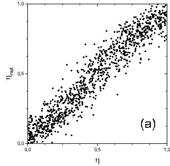
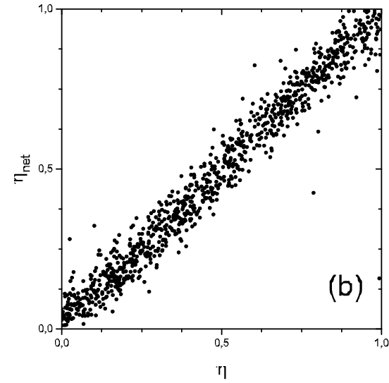
Figure 1: Generalization ability: ANN output $\eta_{\rm net}$ vs the corresponding actual $\eta$ for 1000 MTS spectra in set $G$. In (a) raw data and in (b) Lorentzian fits were used as ANN input.

References

- [1] M.N. Souza, M.A. Figueira and M.S. da Costa, Nucl. Instrum. Methods. Phys. Res. B 73 (1993) 95.
- [2] X. Ni and Y. Hsia, Nuclear Science and Techniques 5 (1994) 162; E.O.T. Salles, P.A. de Souza Jr. and V.K. Garg, Nucl. Instrum. Methods. Phys. Res. B 94 (1994) 499; P.A. de Souza Jr. and V.K. Garg, Czech. J. Phys. 47 (1997) 513; P.A. de Souza Jr., Hyp. Int. 113 (1998) 383; H. Shi, Y. Xiao, H. Huang, D. Wu, A.M. Ali, M. Li, S. Li, Y. Hsia, submitted to Chinese Nucl. Tech. (1999).
- [3] A.X. Trautwein, E. Bill, E.L. Bominaar and H. Winkler, Struct. Bonding 78 (1991) 1.
- [4] M. Haas, E. Realo, H. Winkler, W. Meyer-Klaucke, A. X. Trautwein, O. Leupold and H. D. Rüter, Phys. Rev. B 56 (1997) 14082.
- [5] J. Hertz, A. Krogh, and R.G. Palmer in: introduction to the theory of neural computation, Addison-Wesley, 1991.
- [6] R. Linder and S.J. Pöppl, Neural Computation, in press.
- [7] F. Wagner, Manual for Netfit (Version 1.2), Institut für Theoretische Physik an der Christian-Albrechts-Universität Kiel, Kiel, Germany (1996).
- [8] F. Wagner and C. Lovelace, Nucl. Phys. 25B (1971) 411.