Thermal stability of a weakly magnetized rotating plasma

Abstract

The thermal stability of a weakly magnetized, rotating, stratified, optically thin plasma is studied by means of linear-perturbation analysis. We derive dispersion relations and criteria for stability against axisymmetric perturbations that generalize previous results on either non-rotating or unmagnetized fluids. The implications for the hot atmospheres of galaxies and galaxy clusters are discussed.

1 Introduction

Galaxies and galaxy clusters are embedded in hot atmospheres of virial-temperature gas. The evolution of these systems depends crucially on whether these atmospheres are subject to thermal instability (Parker, 1953; Field, 1965; Defouw, 1970), so that condensations of cold gas can form and grow as a consequence of radiative cooling. Motivated by this astrophysical question, much effort has been devoted to studying the thermal stability of a stratified, optically thin plasma by means of both linear-perturbation analysis (Malagoli, Rosner, & Bodo, 1987; Loewenstein, 1990; Balbus, 1991; Binney, Nipoti & Fraternali, 2009; Balbus & Reynolds, 2008; Balbus & Reynolds, 2010; Nipoti, 2010, hereafter N10) and numerical hydrodynamical simulations (Kaufmann et al., 2009; Joung, Bryan, & Putman, 2012; McCourt et al., 2012; Sharma et al., 2012). The thermal-stability properties of the fluid are influenced by different physical processes. For instance, unmagnetized media behave differently from even weakly magnetized media. Similarly, the stability properties depend significantly on whether the fluid rotates and on the specific rotation law. While the effect of magnetic fields is accounted for in several of the aforementioned works, less attention has been paid to the thermal stability of a rotating stratified plasma. The effect of rotation on the thermal stability, which was discussed in simple cases by Field (1965) and Defouw (1970), has been studied in detail analytically by N10, but only for unmagnetized media (see, e.g., D’Ercole & Ciotti 1998 and Li & Bryan 2012, for a numerical approach).

The rotational properties of the hot gas of galaxies and galaxy clusters are almost unconstrained observationally, because of the relatively poor energy resolution of current X-ray instruments. There are theoretical reasons to expect that rotation is especially important for the coronae of disc galaxies (Marinacci et al., 2011), but some models predict significant rotation also for the hot atmospheres of elliptical galaxies (e.g. Brighenti et al., 2009) and galaxy clusters (e.g. Lau, Kravtsov, & Nagai, 2009). In any case, even if not dynamically dominant, rotation influences the thermal-stability properties of the fluid (N10), as it happens for a subthermal magnetic field (Balbus & Reynolds, 2010). There is observational evidence of the presence of magnetic fields in both the intracluster medium (Carilli & Taylor, 2002) and the gaseous halos of galaxies (Jansson & Farrar, 2012), though the field geometry is still poorly constrained. Notwithstanding these uncertainties on the detailed kinematical and magnetic properties of these gaseous systems, it is clear that allowing for the presence of both rotation and magnetic fields would represent an important step forward in the attempt to understand the thermal stability of the hot atmospheres of galaxies and galaxy clusters.

Here we focus on the problem of the linear stability of a rotating, weakly magnetized plasma against axisymmetric perturbations, accounting for the effects of stratification (i.e. the fluid is in equilibrium in an external gravitational field), differential rotation, radiative cooling and anisotropic thermal conduction. Our analysis can be considered a generalization of previous studies on the linear stability of magnetized fluids. For instance, the non-rotating case has been studied both in the absence (Quataert, 2008; Kunz, 2011) and in the presence (Balbus & Reynolds, 2008; Balbus & Reynolds, 2010; Latter & Kunz, 2012) of radiative losses. The linear stability of a rotating magnetized plasma, in the absence of radiative cooling, has been widely studied in the astrophysical literature, with specific applications to accretion discs (e.g. Balbus & Hawley, 1991, 1992; Urpin & Brandenburg, 1998; Kim & Ostriker, 2000; Brandenburg & Dintrans, 2006; Islam, 2012; Salhi et al., 2012) and rotating stars (e.g. Fricke, 1969; Pitts & Tayler, 1985; Menou, Balbus, & Spruit, 2004; Masada, 2011). The stability-analysis techniques developed in these works, as well as in studies of rotating unmagnetized media (see N10, and references therein), can be applied to the more general problem addressed here.

It is worth spending a few words on the structure of the magnetic field, which, as already mentioned, is poorly constrained observationally. Throughout this work we will assume that, at least from the point of view of the perturbation, the magnetic field is ordered. This does not necessarily imply that the magnetic field is ordered over scales comparable to the size of the system: the field may as well be tangled, but with coherence length substantially larger than the size of the perturbation. If, instead, the coherence length of the field is comparable to or smaller than the size of the perturbation, the system is better described by an unmagnetized model (such as that of  N10) in which thermal conduction is suppressed by some factor, accounting for the effect of the tangled magnetic field (see, e.g., Binney et al. 2009, for a discussion).

The paper is organized as follows. In Section 2 we describe the plasma model and we derive the general dispersion relation for linear axisymmetric perturbations. Stability criteria for previously studied limiting cases are obtained in Section 3. In Section 4 we present our new stability criteria. In Section 5 we summarize our main results and discuss the implications for the hot atmospheres of galaxies and galaxy clusters.

2 Linear-perturbation analysis

2.1 Governing equations

A stratified, rotating, magnetized atmosphere in the presence of thermal conduction and radiative cooling is governed by the following magnetohydrodynamics equations:

$${\partial\rho\over\partial t}+{\nabla}\cdot(\rho{\bf v})=0,$$ (1)

$$\rho\left[{\partial{\bf v}\over\partial t}+\left({\bf v}\cdot{\nabla}\right){\bf v}\right]=-{\nabla}\left(p+{B^{2}\over 8\pi}\right)-\rho{\nabla}\Phi+{1\over 4\pi}({\bf B}\cdot\nabla){\bf B},$$ (2)

$${\partial{\bf B}\over\partial t}-\nabla\times({\bf v}\times{\bf B})=0,$$ (3)

$${p\over\gamma-1}\left[{\partial\over\partial t}+{\bf v}\cdot{\nabla}\right]\ln(p\rho^{-\gamma})=-{\nabla}\cdot{\bf Q}-\rho\mathcal{L},$$ (4)

supplemented by the condition that the magnetic field ${\bf B}$ is solenoidal ($\nabla\cdot{\bf B}=0$). Here $\rho$, $p$, $T$ and ${\bf v}$ are, respectively, the density, pressure, temperature and velocity fields of the fluid, $B\equiv|{\bf B}|$, $\Phi$ is the external gravitational potential (we neglect self-gravity), $\gamma$ is the adiabatic index, ${\bf Q}$ is the conductive heat flux, and $\mathcal{L}=\mathcal{L}(T,\rho)$ is the radiative energy loss per unit mass of fluid. In a dilute magnetized plasma heat is significantly transported by electrons only along magnetic force lines (see Braginskii, 1965). In other words, in the presence of a magnetic field the thermal conduction is anisotropic, so the conductive heat flux is given by

$${\bf Q}=-\frac{\chi{\bf B}\left({\bf B}\cdot\nabla\right)T}{B^{2}},$$ (5)

where $\chi$ is the Spitzer electron conductivity that can be expressed as

$$\chi\equiv\kappa T^{5/2},$$ (6)

with $\kappa\simeq{1.84\times 10^{-5}(\ln{\Lambda})}^{-1}\,{\rm erg}\,{\rm s}^{-1}\,{\rm cm}^{-1}\,{\rm K}^{-7/2}$, and $\ln\Lambda$ is the Coulomb logarithm (Spitzer, 1962). In the following we neglect the weak temperature and density dependence of $\ln\Lambda$, assuming that $\kappa$ is a constant, so $\chi=\chi(T)\propto T^{5/2}$. In the unmagnetized case thermal conduction is isotropic, i.e. the heat flux is

$${\bf Q}=-\kappa T^{5/2}\nabla T.$$ (7)

Thermal conduction in the presence of a magnetic field is therefore reduced in directions that are not parallel to the field lines, and it is null in the direction orthogonal to the field. It follows that the effect of a tangled magnetic field is, in general, a suppression of heat conduction: in a first approximation the presence of a tangled magnetic field can be modeled as an unmagnetized medium with a scalar thermal conduction (equation 7), but with $\kappa$ reduced by some factor (Binney & Cowie, 1981). However, if the coherence length of the tangled field is substantially larger than the size of the perturbation, the anisotropy of the conductivity becomes crucial for the stability properties of the magnetized medium (Balbus, 2001; Quataert, 2008). In the following we will focus on the latter case and we will consider the anisotropic heat flux as given in equation (5).

In cylindrical coordinates $(R,\phi,z)$, neglecting all derivatives with respect to $\phi$ (because we will consider only axisymmetric unperturbed fields and disturbances), the governing equations (1-4) read

$$\displaystyle\frac{\partial\rho}{\partial t}+\frac{1}{R}\frac{\partial R\rho{v_{R}}}{\partial R}+\frac{\partial\rho{v_{z}}}{\partial z}=0,$$ (8)

$$\displaystyle\frac{\partial{v_{R}}}{\partial t}+{v_{R}}\frac{\partial{v_{R}}}{\partial R}+{v_{z}}\frac{\partial{v_{R}}}{\partial z}-\frac{v_{\phi}^{2}}{R}=-\frac{1}{\rho}\frac{\partial p}{\partial R}-\frac{\partial\Phi}{\partial R}+\frac{1}{4\pi\rho}\left(B_{R}\frac{\partial B_{R}}{\partial R}+B_{z}\frac{\partial B_{R}}{\partial z}-\frac{B_{\phi}^{2}}{R}\right)-\frac{1}{8\pi\rho}\frac{\partial B^{2}}{\partial R},$$ (9)

$$\displaystyle\frac{\partial v_{\phi}}{\partial t}+{v_{R}}\frac{\partial v_{\phi}}{\partial R}+{v_{z}}\frac{\partial v_{\phi}}{\partial z}+\frac{{v_{R}}v_{\phi}}{R}=\frac{1}{4\pi\rho}\left(B_{R}\frac{\partial B_{\phi}}{\partial R}+B_{z}\frac{\partial B_{\phi}}{\partial z}+\frac{B_{R}B_{\phi}}{R}\right),$$ (10)

$$\displaystyle\frac{\partial{v_{z}}}{\partial t}+{v_{R}}\frac{\partial{v_{z}}}{\partial R}+{v_{z}}\frac{\partial{v_{z}}}{\partial z}=-\frac{1}{\rho}\frac{\partial p}{\partial z}-\frac{\partial\Phi}{\partial z}+\frac{1}{4\pi\rho}\left(B_{R}\frac{\partial B_{z}}{\partial R}+B_{z}\frac{\partial B_{z}}{\partial z}\right)-\frac{1}{8\pi\rho}\frac{\partial B^{2}}{\partial z},$$ (11)

$$\displaystyle\frac{\partial B_{R}}{\partial t}=B_{R}\frac{\partial{v_{R}}}{\partial R}+B_{z}\frac{\partial{v_{R}}}{\partial z}-{v_{R}}\frac{\partial B_{R}}{\partial R}-{v_{z}}\frac{\partial B_{R}}{\partial z}-(\nabla\cdot{\bf v})B_{R},$$ (12)

$$\displaystyle\frac{\partial B_{\phi}}{\partial t}=B_{R}\frac{\partial v_{\phi}}{\partial R}+B_{z}\frac{\partial v_{\phi}}{\partial z}+\frac{B_{\phi}{v_{R}}}{R}-{v_{R}}\frac{\partial B_{\phi}}{\partial R}-{v_{z}}\frac{\partial B_{\phi}}{\partial z}-\frac{v_{\phi}B_{R}}{R}-(\nabla\cdot{\bf v})B_{\phi},$$ (13)

$$\displaystyle\frac{\partial B_{z}}{\partial t}=B_{R}\frac{\partial{v_{z}}}{\partial R}+B_{z}\frac{\partial{v_{z}}}{\partial z}-{v_{R}}\frac{\partial B_{z}}{\partial R}-{v_{z}}\frac{\partial B_{z}}{\partial z}-(\nabla\cdot{\bf v})B_{z},$$ (14)

$$\displaystyle\frac{p}{\gamma-1}\left(\frac{\partial}{\partial t}+{v_{R}}\frac{\partial}{\partial R}+{v_{z}}\frac{\partial}{\partial z}\right)\ln(p\rho^{-\gamma})=\frac{1}{R}\frac{\partial}{\partial R}\left[R\frac{\chi(T)B_{R}({\bf B}\cdot\nabla)T}{B^{2}}\right]+\frac{\partial}{\partial z}\left[\frac{\chi(T)B_{z}({\bf B}\cdot\nabla)T}{B^{2}}\right]-\rho\mathcal{L}(T,\rho),$$ (15)

where we have used $\nabla\cdot{\bf B}=0$ in writing the three components (equations 12-14) of the induction equation (3).

2.2 The unperturbed plasma

The unperturbed system is described by time-independent axisymmetric pressure ${p_{0}}$, density $\rho_{0}$, temperature $T_{0}$, velocity ${\bf v}_{0}=(v_{0R},v_{0\phi},v_{0z})$ and magnetic field ${\bf B}_{0}=(B_{0R},B_{0\phi},B_{0z})$ satisfying equations (8-15) with vanishing partial derivatives with respect to $t$, under the assumption that the plasma is weakly magnetized, in the sense that the parameter $\beta\equiv 8\pi{p_{0}}/B_{0}^{2}\gg 1$, where $B_{0}\equiv|{\bf B}_{0}|$: in other words, the magnetic field is subthermal and dynamically unimportant. Formally, such a steady-state configuration requires that, in the unperturbed system, cooling is perfectly balanced by heat conduction, which appears like an artificial and unrealistic assumption. However, the steady-state solution can be interpreted more broadly as describing a “quasi-stationary” state, which does not evolve significantly over the timescales of interest and is close to hydrostatic and thermal equilibrium. So, globally, the cooling time of the system is assumed to be much longer than the dynamical time, which is clearly the case for the hot atmospheres of galaxies and galaxy clusters.

The unperturbed fluid is allowed to rotate differentially with angular velocity $\Omega(R,z)\equiv v_{0\phi}(R,z)/R$ depending on both $R$ and $z$. Without loss of generality we choose our azimuthal coordinate $\phi$ so that $\Omega\geq 0$. We assume that there is no meridional circulation in the background fluid. In principle the velocity components $v_{0R}$ and $v_{0z}$ could be non-null, even in the absence of meridional circulation, because a time-independent subsonic inflow of gas can occur if cooling is not perfectly balanced by thermal conduction (see, e.g., N10). However, for simplicity, in the present investigation we limit ourselves to the case $v_{0R}=v_{0z}=0$. It must be noted that the Poincaré-Wavre theorem (Tassoul, 1978), which holds for unmagnetized fluids, applies also to our model of magnetized plasma, as long as the magnetic field is dynamically unimportant in the unperturbed configuration ($\beta\gg 1$). Therefore, the fluid is baroclinic [i.e. $p=p(\rho,T)$] in the general case in which $\Omega=\Omega(R,z)$, and is barotropic [i.e. $p=p(\rho)$] only in the particular case in which the angular velocity is constant on cylinders [$\Omega=\Omega(R)$].

A useful relation among unperturbed quantities is the vorticity equation, which is derived from the momentum equations and, under the above hypotheses, can be written as

$$R\frac{\partial\Omega^{2}}{\partial z}=\frac{1}{\rho_{0}T_{0}}\left(\frac{\partial T_{0}}{\partial z}\frac{\partial{p_{0}}}{\partial R}-\frac{\partial T_{0}}{\partial R}\frac{\partial{p_{0}}}{\partial z}\right).$$ (16)

As we have assumed that there are no motions in the meridional plane ($v_{0R}=v_{0z}=0$), in the hypothesis that all components of the background magnetic fields are time-independent the induction equation implies that the unperturbed system satisfies Ferraro’s isorotation law (Ferraro, 1937)

$${\bf B}_{0}\cdot\nabla\Omega=0,$$ (17)

i.e. the angular velocity is constant along field lines (see equation 13). It has been noted (Balbus & Hawley, 1991) that condition (17) might be too restrictive when the magnetic field is weak. If ${\bf B}_{0}\cdot\nabla\Omega\neq 0$ the azimuthal component $B_{0\phi}$ of the magnetic field varies secularly (see equation 13), but, provided that the magnetic field remains subthermal, the time dependence of $B_{0\phi}$ does not imply the time dependence of any of the other unperturbed fields. So it is possible to consider a more general unperturbed weak-field configuration, in which condition (17) is not satisfied, $B_{0\phi}$ depends on time, while all the other unperturbed quantities (including $B_{0R}$ and $B_{0z}$) are time-independent: the results of the perturbation analysis are still valid in this case, provided the dispersion relation does not depend on $B_{0\phi}$. It turns out that this is not the case for the most general dispersion relation derived in the present work (see Section 2.3), so we will limit ourselves to the case ${\bf B}_{0}\cdot\nabla\Omega=0$.

2.3 Dispersion relation for axisymmetric perturbations

We describe here the linear-perturbation analysis of the weakly magnetized, stratified, dissipative fluid governed by the equations reported in Section 2.1, assuming a background configuration as described in Section 2.2. In practice, we linearize the system (8)-(15) by using axisymmetric Eulerian perturbations of the form $\displaystyle{f_{0}}+f{\rm e}^{-{\rm i}\omega t+{\rm i}k_{R}R+{\rm i}k_{z}z}$, where ${f_{0}}$ is the unperturbed quantity, $|f|\ll|{f_{0}}|$, $\omega$ is the perturbation frequency, and $k_{R}$ and $k_{z}$ are, respectively, the radial and vertical components of the perturbation wavevector. The linear analysis is intended to be taken locally in the plasma, in the sense that the perturbation wavelength is much shorter than the characteristic scalelengths of the unperturbed system. We further assume that the perturbation frequency is much lower than the sound-wave frequency, so we work in the Boussinesq approximation to exclude a priori the (stable) modes describing the sound waves. In linearizing the thermal conduction term, it is useful to note that the linear perturbation of the heat flux, in the Wentzel-Kramers-Brillouin (WKB) approximation, is

$${\bf Q}=-\chi(T_{0})\left[{\bf b}_{0}({\bf b}_{0}\cdot\nabla)T+{\bf b}_{0}({\bf b}\cdot\nabla)T_{0}+{\bf b}({\bf b}_{0}\cdot\nabla)T_{0}-2{\bf b}_{0}({\bf b}_{0}\cdot{\bf b})({\bf b}_{0}\cdot\nabla)T_{0}\right],$$ (18)

where we have introduced the dimensionless vectors ${\bf b}\equiv{\bf B}/B_{0}$ and ${\bf b}_{0}\equiv{\bf B}_{0}/B_{0}$. From the above expression, writing explicitly the axisymmetric perturbation, we obtain the thermal-conduction term of the linearized energy equation:

$$-\nabla\cdot{\bf Q}=\chi(T_{0})T_{0}\left[-({\bf k}\cdot{\bf b}_{0})^{2}{T\over T_{0}}+{\rm i}({\bf k}\cdot{\bf b}_{0})(\nabla\ln T_{0}\cdot{\bf b})+{\rm i}(\nabla\ln T_{0}\cdot{\bf b}_{0})({\bf k}\cdot{\bf b})-2{\rm i}({\bf b}_{0}\cdot{\bf k})(\nabla\ln T_{0}\cdot{\bf b}_{0})({\bf b}_{0}\cdot{\bf b})\right],$$ (19)

where ${\bf k}=(k_{R},0,k_{z})$, because $k_{\phi}=0$ for axisymmetric disturbances. The first term in the right-hand side of equation (19) is similar to what is obtained in the case of unmagnetized heat flux (equation 7), but accounts for the relative orientation of the displacement and the unperturbed magnetic field. The second term leads to the so-called magnetothermal instability (MTI; Balbus 2001). The third and fourth terms lead to the so-called heat-flux driven buoyant instability (HBI; Quataert 2008): we recall that these latter two terms are null if one makes the assumption of isothermal unperturbed magnetic field lines ($\nabla T_{0}\cdot{\bf b}_{0}=0$), which implies that there is no heat flux in the unperturbed medium. In the present framework, in which the gas is allowed to cool, we are interested in the more general case $\nabla T_{0}\cdot{\bf b}_{0}\neq 0$, the underlying assumption being that the timescale of the background heat flux is long as compared to the local dynamical time. It must be noted that, even when radiative cooling is negligible, the assumption of isothermal field lines is not necessary: formally, the unperturbed system can be in steady state also when $\nabla T_{0}\cdot{\bf b}_{0}\neq 0$, provided that the divergence of the heat flux vanishes (see Quataert 2008, for a discussion).

Linearizing the system of partial differential equations (8-15), assuming axisymmetric perturbations in the WKB approximation, we get the following system of linear equations:

$$\displaystyle{\rm i}k_{R}{v_{R}}+{\rm i}k_{z}{v_{z}}=0,$$ (20)

$$\displaystyle-{\rm i}\omega{v_{R}}\rho_{0}+{\rm i}k_{R}p-2\Omega v_{\phi}\rho_{0}-c_{0}^{2}A_{pR}\rho-\frac{{\rm i}k_{z}B_{0z}}{4\pi}B_{R}+\frac{{\rm i}k_{R}}{4\pi}(B_{0\phi}B_{\phi}+B_{0z}B_{z})=0,$$ (21)

$$\displaystyle-{\rm i}\omega v_{\phi}\rho_{0}+(\Omega+\Omega_{R}){v_{R}}\rho_{0}+\Omega_{z}{v_{z}}\rho_{0}-\frac{{\rm i}({\bf k}\cdot{\bf B}_{0})}{4\pi}B_{\phi}=0,$$ (22)

$$\displaystyle-{\rm i}\omega{v_{z}}\rho_{0}+{\rm i}k_{z}p-c_{0}^{2}A_{pz}\rho-\frac{{\rm i}k_{R}B_{0R}}{4\pi}B_{z}+\frac{{\rm i}k_{z}}{4\pi}(B_{0\phi}B_{\phi}+B_{0R}B_{R})=0,$$ (23)

$$\displaystyle-{\rm i}\omega B_{R}-{\rm i}({\bf k}\cdot{\bf B}_{0}){v_{R}}=0,$$ (24)

$$\displaystyle-{\rm i}\omega B_{\phi}-{\rm i}({\bf k}\cdot{\bf B}_{0})v_{\phi}-(\Omega_{R}-\Omega)B_{R}-\Omega_{z}B_{z}=0,$$ (25)

$$\displaystyle-{\rm i}\omega B_{z}-{\rm i}({\bf k}\cdot{\bf B}_{0}){v_{z}}=0,$$ (26)

$$\displaystyle{1\over\gamma}\left[{\rm i}\gamma\omega\frac{\rho}{\rho_{0}}+{v_{R}}(A_{pR}-\gamma A_{\rho{R}})+{v_{z}}(A_{pz}-\gamma A_{\rho{z}})\right]=$$

$$\displaystyle\qquad=-\omega_{\rm d}{T\over T_{0}}+{\rm i}\left({\gamma-1\over\gamma}\right){\chi(T_{0})T_{0}\over{p_{0}}}\left[({\bf k}\cdot{\bf b}_{0})\nabla\ln T_{0}+(\nabla\ln T_{0}\cdot{\bf b}_{0}){\bf k}-2({\bf k}\cdot{\bf b}_{0})(\nabla\ln T_{0}\cdot{\bf b}_{0}){\bf b}_{0}\right]\cdot{\bf b},$$ (27)

where $c_{0}^{2}\equiv{p_{0}}/\rho_{0}$ is the isothermal sound speed squared; the quantities $A_{pR}\equiv(\partial{p_{0}}/\partial R)/{p_{0}}$ [$A_{\rho{R}}\equiv(\partial\rho_{0}/\partial R)/\rho_{0}$] and $A_{pz}\equiv(\partial{p_{0}}/\partial z)/{p_{0}}$ [$A_{\rho{z}}\equiv(\partial\rho_{0}/\partial z)/\rho_{0}$] are the inverse of the pressure (density) scale-length and scale-height, respectively. In analogy with N10 we have defined

$$\omega_{\rm d}\equiv\begin{cases}\omega_{\rm c}+\omega_{\rm th}&\text{if $B_{0}=0$,}\\ \omega_{\rm c,a}+\omega_{\rm th}&\text{if $B_{0}\neq 0$,}\end{cases}$$ (28)

where

$$\omega_{\rm c}\equiv\left({\gamma-1\over\gamma}\right){k^{2}\chi(T_{0})T_{0}\over{p_{0}}}$$ (29)

is the isotropic thermal-conduction frequency,

$$\omega_{\rm c,a}\equiv\frac{({\bf k}\cdot{\bf b}_{0})^{2}}{k^{2}}\omega_{\rm c}$$ (30)

is the anisotropic thermal-conduction frequency, and

$$\omega_{\rm th}\equiv-\left({\gamma-1\over\gamma}\right)\frac{\rho_{0}}{{p_{0}}}\left[\mathcal{L}(\rho_{0},T_{0})+\rho_{0}\mathcal{L}_{\rho}(\rho_{0},T_{0})-T_{0}\mathcal{L}_{T}(\rho_{0},T_{0})\right]$$ (31)

is the thermal-instability frequency with $\mathcal{L}_{\rho}\equiv{\partial\mathcal{L}}/{\partial\rho}$ and $\mathcal{L}_{T}\equiv{\partial\mathcal{L}}/{\partial T}$; $\Omega_{R}\equiv\partial(\Omega R)/\partial R$ and $\Omega_{z}\equiv\partial(\Omega R)/\partial z$ are two frequencies associated with the angular velocity gradient. In terms of the defined quantities, the assumption of short-wavelength perturbations gives $|k_{R}|,|k_{z}|\gg|A_{\rho{R}}|,|A_{\rho{z}}|,|A_{pz}|,|A_{pR}|$, and $\Omega^{2},\Omega_{R}^{2},\Omega_{z}^{2}\ll c_{0}^{2}k^{2}$, while the assumption of low-frequency perturbations gives $\omega^{2}\ll c_{0}^{2}k^{2}$. As implementations of the Boussinesq approximation we neglected the term $-{\rm i}\omega\rho/\rho_{0}$ in the mass-conservation equation and the term $-{\rm i}\omega p/{p_{0}}$ in the energy equation, and we assumed $\rho_{0}T\simeq-T_{0}\rho$ (see N10, ). We recall that the magnetic field is considered weak ($\beta\gg 1$): in particular we assumed $\beta$ of the order of $(k/|A_{\rho{R}}|)^{2}$.

The system of linear equations (20-27) can be reduced to the following $5$-th order dispersion relation for $n\equiv-{\rm i}\omega$:

$$\begin{array}[]{c}\displaystyle n^{5}+\omega_{\rm d}n^{4}+\left[\omega^{2}_{\rm BV}+\omega^{2}_{\rm rot}+2\omega^{2}_{\rm A}\right]n^{3}+\left[(\omega^{2}_{\rm rot}+2\omega^{2}_{\rm A})\omega_{\rm d}+\omega^{2}_{\rm A}\omega_{\rm c,mag}\right]n^{2}+\\ \displaystyle\quad\,\,+\omega^{2}_{\rm A}\left(\omega^{2}_{\rm A}+\omega^{2}_{\rm BV}+\omega^{2}_{\rm rot}-4\Omega^{2}\frac{k_{z}^{2}}{k^{2}}+\omega^{2}_{\rm c,\phi}\right)n+\omega^{2}_{\rm A}\left[\left(\omega^{2}_{\rm A}+\omega^{2}_{\rm rot}-4\Omega^{2}\frac{k_{z}^{2}}{k^{2}}\right)\omega_{\rm d}+\omega^{2}_{\rm A}\omega_{\rm c,mag}\right]=0.\end{array}$$ (32)

This is the most general dispersion relation derived in the present work, describing the evolution of axisymmetric perturbations in a gravitationally stratified, rotating, plasma subject to radiative cooling and thermal conduction, in the presence of a weak magnetic field of arbitrary geometry. Here, as in N10, we have introduced the quantity

$$\omega^{2}_{\rm rot}\equiv-{k_{z}^{2}\over k^{2}}{1\over R^{3}}\mathcal{D}({R^{4}\Omega^{2}}),$$ (33)

which is the square of the frequency associated with differential rotation, and the Brunt-Väisälä (buoyancy) frequency $\omega_{\rm BV}$, defined by

$$\omega^{2}_{\rm BV}\equiv-{k_{z}^{2}\over k^{2}}{\mathcal{D}{p_{0}}\over\rho_{0}\gamma}\mathcal{D}{s_{0}},$$ (34)

where ${s_{0}}\equiv\ln{p_{0}}\rho_{0}^{-\gamma}$ is the unperturbed specific entropy and

$$\mathcal{D}\equiv{k_{R}\over k_{z}}{\partial\over\partial z}-{\partial\over\partial R}$$ (35)

is a differential operator which takes derivatives along surfaces of constant wave phase (Balbus, 1995). In addition we have introduced the Alfvén frequency $\omega_{\rm A}\equiv{\bf k}\cdot{\bf v}_{\rm A}$, where $\displaystyle{\bf v}_{\rm A}\equiv{{\bf B}_{0}}/{\sqrt{4\pi\rho_{0}}}$ is the Alfvén velocity, and the following frequencies related to the anisotropy of the thermal conduction due to the presence of a magnetic field:

$$\omega_{\rm c,mag}\equiv-\omega_{\rm c}\frac{4\pi{p_{0}}}{B_{0}^{2}}{k_{z}^{2}\over k^{2}}\frac{\mathcal{D}\ln{p_{0}}}{k^{2}}\left[\mathcal{D}\ln T_{0}-2\left(\nabla\ln T_{0}\cdot{\bf b}_{0}\right)\left(\frac{k_{R}}{k_{z}}{b_{0z}}-b_{0R}\right)\right],$$ (36)

which is in general non-null for any geometry of the unperturbed magnetic field, and $\omega_{\rm c,\phi}$, defined by

$$\omega^{2}_{\rm c,\phi}\equiv\omega_{\rm c}\Omega\frac{8\pi{p_{0}}}{B_{0}^{2}}{k_{z}^{2}\over k^{2}}\frac{\mathcal{D}\ln{p_{0}}}{k^{2}}(\nabla\ln T_{0}\cdot{\bf b}_{0})b_{0\phi},$$ (37)

which can be non-vanishing only if the magnetic field has a non-vanishing azimuthal component ($b_{0\phi}\neq 0$). We note that the dispersion relation (32) depends on $B_{0\phi}$ through the quantities $b_{0\phi}$, $b_{0R}$ and $b_{0z}$, so we will restrict our analysis to unperturbed configurations with isorotational magnetic field (${\bf B}_{0}\cdot\nabla\Omega=0$), for which $B_{0\phi}$ is time-independent (see discussion at the end of Section 2.2).

We recall that, in terms of the quantity $n$ appearing in the dispersion relation (32), the perturbation evolves with a time dependence $f(t)\propto{\rm e}^{nt}$, where in general $n\in\mathbb{C}$. Therefore, stable modes are those with ${\rm Re}(n)\leq 0$ and unstable modes those with ${\rm Re}(n)>0$. Among the unstable modes it is useful to distinguish between purely unstable modes, having ${\rm Im}(n)=0$, in which the perturbation grows monotonically, and overstable modes, having ${\rm Im}(n)\neq 0$, in which the perturbation oscillates with exponentially growing amplitude. We also remind the reader that, while $\omega_{\rm A}^{2}\geq 0$ for all ${\bf k}$, the quantities $\omega^{2}_{\rm rot}$, $\omega^{2}_{\rm BV}$ and $\omega^{2}_{\rm c,\phi}$ can be either positive or negative, also depending on ${\bf k}$. A list of definitions of some relevant quantities used in the present work is given for reference in Table 1.

Table 1: List of definitions.

$A_{pR}\equiv\frac{\partial\ln{p_{0}}}{\partial R}$,   $A_{pz}\equiv\frac{\partial\ln{p_{0}}}{\partial z}$,   $A_{\rho{R}}\equiv\frac{\partial\ln\rho_{0}}{\partial R}$,   $A_{\rho{z}}\equiv\frac{\partial\ln\rho_{0}}{\partial z}$,

$c_{0}\equiv\left(\frac{{p_{0}}}{\rho_{0}}\right)^{1/2}$,   $\mathcal{D}\equiv{\frac{k_{R}}{k_{z}}}\frac{\partial}{\partial z}-\frac{\partial}{\partial R}$,   $n\equiv-{\rm i}\omega$,   ${s_{0}}\equiv\ln{p_{0}}\rho_{0}^{-\gamma}$,

$\omega^{2}_{\rm A}\equiv({\bf k}\cdot{\bf v}_{\rm A})^{2}=\frac{({\bf k}\cdot{{\bf B}_{0}})^{2}}{4\pi\rho_{0}}$,   $\omega^{2}_{\rm BV}\equiv-{k_{z}^{2}\over k^{2}}{\mathcal{D}{p_{0}}\over\rho_{0}\gamma}\mathcal{D}{s_{0}}$,   $\omega_{\rm c}\equiv\left({\gamma-1\over\gamma}\right){k^{2}\chi(T_{0})T_{0}\over{p_{0}}}$,   $\omega_{\rm c,a}\equiv\frac{({\bf k}\cdot{\bf b}_{0})^{2}}{k^{2}}\omega_{\rm c}$,

$\omega_{\rm c,mag}\equiv-\omega_{\rm c}\frac{4\pi{p_{0}}}{B_{0}^{2}}{k_{z}^{2}\over k^{2}}\frac{\mathcal{D}\ln{p_{0}}}{k^{2}}\left[\mathcal{D}\ln T_{0}-2\left(\nabla\ln T_{0}\cdot{\bf b}_{0}\right)\left(\frac{k_{R}}{k_{z}}{b_{0z}}-b_{0R}\right)\right]$,   $\omega^{2}_{\rm c,\phi}\equiv\omega_{\rm c}\Omega\frac{8\pi{p_{0}}}{B_{0}^{2}}{k_{z}^{2}\over k^{2}}\frac{\mathcal{D}\ln{p_{0}}}{k^{2}}(\nabla\ln T_{0}\cdot{\bf b}_{0})b_{0\phi}$,

$\omega^{2}_{\rm rot}\equiv-{k_{z}^{2}\over k^{2}}{1\over R^{3}}\mathcal{D}({R^{4}\Omega^{2}})$,   $\omega_{\rm th}\equiv-\left({\gamma-1\over\gamma}\right)\frac{\rho_{0}}{{p_{0}}}\left[\mathcal{L}(\rho_{0},T_{0})+\rho_{0}\mathcal{L}_{\rho}(\rho_{0},T_{0})-T_{0}\mathcal{L}_{T}(\rho_{0},T_{0})\right]$,

$\omega_{\rm d}\equiv\omega_{\rm th}+\omega_{\rm c,a}$ (if $B_{0}\neq 0$),   $\omega_{\rm d}\equiv\omega_{\rm th}+\omega_{\rm c}$ (if $B_{0}=0$),  $\Omega_{R}\equiv\frac{\partial(\Omega R)}{\partial R}$,  $\Omega_{z}\equiv\frac{\partial(\Omega R)}{\partial z}$,  $\alpha\equiv\frac{2\Omega^{2}\rho_{0}{p_{0}}}{|\nabla{p_{0}}|^{2}}$

3 Stability criteria in limiting cases: comparison with previous studies

Before investigating the stability conditions for the dispersion relation (32) in its general form, it is convenient to discuss some simpler cases that have been already studied in the astrophysical literature. In particular we analyze here the limiting cases of the dispersion relation (32) in which at least one among $\omega_{\rm A}$, $\omega_{\rm th}$ and $\Omega$ is zero. In all cases we account for the effect of thermal conduction on the stability of the plasma. This preliminary analysis is propaedeutic to Section 4, where we present new stability criteria, because it helps simplify the derivation and the interpretation of the results of the more general cases discussed there. In this Section, as well as in Section 4, for a given dispersion relation we obtain necessary and sufficient conditions for stability following the approach described in Appendix A, which is based on the Routh-Hurwitz theorem for the stability of polynomials.

3.1 Unmagnetized, rotating, radiatively cooling plasma ($\Omega\neq 0$, $\omega_{\rm A}=0$, $\omega_{\rm th}\neq 0$)

When the Alfvén frequency $\omega_{\rm A}=0$ the dispersion relation (32) reduces to

$$n^{3}+n^{2}\omega_{\rm d}+(\omega^{2}_{\rm BV}+\omega^{2}_{\rm rot})n+\omega^{2}_{\rm rot}\omega_{\rm d}=0,$$ (38)

which was obtained by N10 for an unmagnetized rotating plasma. We note that the condition $\omega_{\rm A}=0$ is achieved not only if the fluid is unmagnetized, but whenever the projection of the magnetic field onto the wavevector is zero. For example, the dispersion relation (38) is obtained also for a system subject to an azimuthal magnetic field ($B_{0\phi}\neq 0$, $B_{0R}=B_{0z}=0$), perturbed with linear axisymmetric disturbances. In this azimuthal magnetic field configuration thermal conduction is ineffective ($\omega_{\rm d}=\omega_{\rm th}$), in contrast with the unmagnetized case in which ($\omega_{\rm d}=\omega_{\rm c}+\omega_{\rm th}$), but in both cases the dispersion relation is formally identical to the most general dispersion relation found in N10 for axisymmetric perturbations. Performing a stability analysis of equation (38) as described in Appendix A, we obtain the necessary and sufficient stability criterion

$$\omega_{\rm d}\geq 0,\qquad\omega^{2}_{\rm rot}\geq 0,\qquad\omega^{2}_{\rm BV}\geq 0,$$ (39)

as found in N10 (see figure 1 in that paper). For the above criterion to be satisfied for all wavevectors the following conditions must hold:

$$\omega_{\rm th}\geq 0,\qquad\nabla{p_{0}}\cdot\nabla{s_{0}}\leq 0,\quad\frac{\partial\Omega}{\partial z}=0,\quad\frac{\partial(\Omega R^{2})}{\partial R}\geq 0.$$ (40)

So, we have stability only for barotropic fluids [$\Omega=\Omega(R)$] satisfying the Field ($\omega_{\rm th}\geq 0$), Schwarzschild (${\rm d}{s_{0}}/{\rm d}{p_{0}}\leq 0$) and Rayleigh ${\rm d}(\Omega R^{2})/{\rm d}R\geq 0$ criteria. When these conditions are not satisfied we can have either monotonically growing instability or overstability (see N10, ).

3.2 Magnetized, non-rotating plasma without radiative cooling ($\Omega=0$, $\omega_{\rm A}\neq 0$, $\omega_{\rm th}=0$)

Here the fluid is magnetized but it does not rotate and there is no cooling. This is the case considered in Cartesian coordinates by Quataert (2008). We still work in cylindrical coordinates, but, without loss of generality, we assume $B_{0\phi}=0$ (so $b_{0R}^{2}+b_{0z}^{2}=1$). The dispersion relation (32) becomes

$$\left(n^{2}+\omega^{2}_{\rm A}\right)\left[n^{3}+\omega_{\rm c,a}n^{2}+\left(\omega^{2}_{\rm A}+\omega^{2}_{\rm BV}\right)n+\omega^{2}_{\rm A}\left(\omega_{\rm c,a}+\omega_{\rm c,mag}\right)\right]=0.$$ (41)

The zeroes of the quadratic factor are $n=\pm{\rm i}\omega_{\rm A}$: the two oscillatory solutions describing the Alfvén waves. Applying the stability analysis (see Appendix A) to the cubic factor we first get the following two necessary conditions for stability:

$$\Delta_{2}\geq 0\iff\omega_{\rm c,a}\omega^{2}_{\rm BV}-\omega_{\rm c,mag}\omega^{2}_{\rm A}\geq 0,$$ (42)

$$\Delta_{3}\geq 0\iff\omega^{2}_{\rm A}(\omega_{\rm c,a}\omega^{2}_{\rm BV}-\omega_{\rm c,mag}\omega^{2}_{\rm A})(\omega_{\rm c,mag}+\omega_{\rm c,a})\geq 0,$$ (43)

because $\Delta_{1}=\omega_{\rm c,a}\geq 0$ for all ${\bf k}$. The condition on $\Delta_{2}$ can be rearranged as

$$\mathcal{D}{p_{0}}\left[-{1\over\gamma}\mathcal{D}{s_{0}}+\mathcal{D}\ln T_{0}-2\left(\nabla\ln T_{0}\cdot{\bf b}_{0}\right)\left(\frac{k_{R}}{k_{z}}b_{0z}-b_{0R}\right)\right]\geq 0.$$ (44)

Using the identity ${\mathcal{D}{s_{0}}}=\gamma\mathcal{D}\ln T_{0}-(\gamma-1)\mathcal{D}\ln{p_{0}}$, it is possible to write the condition (44) as

$$\frac{\gamma-1}{\gamma}\frac{1}{{p_{0}}}\left(\mathcal{D}{p_{0}}\right)^{2}-2\mathcal{D}{p_{0}}\left(\nabla\ln T_{0}\cdot{\bf b}_{0}\right)\left(\frac{k_{R}}{k_{z}}b_{0z}-b_{0R}\right)\geq 0.$$ (45)

We note that in the absence of rotation the fluid is barotropic, so surfaces of constant density, pressure and temperature coincide (see Section 2.2), and, without loss of generality, we can assume ${p_{0}}={p_{0}}(z)$ and $T_{0}=T_{0}(z)$, so that $\mathcal{D}=x{\rm d}/{\rm d}z$, where $x\equiv k_{R}/k_{z}$. Requiring for stability the validity of the inequality (45) $\forall x$, we get the following two conditions for stability:

$$b_{0z}b_{0R}\frac{{\rm d}T_{0}}{{\rm d}z}\frac{{\rm d}{p_{0}}}{{\rm d}z}=0,\qquad\frac{{\rm d}{p_{0}}}{{\rm d}z}\left(\frac{\gamma-1}{\gamma}\frac{{\rm d}\ln{p_{0}}}{{\rm d}z}-2b_{0z}^{2}\frac{{\rm d}\ln T_{0}}{{\rm d}z}\right)\geq 0.$$ (46)

When $\Delta_{2}\geq 0$ the condition $\Delta_{3}\geq 0$ becomes $\omega_{\rm c,a}+\omega_{\rm c,mag}\geq 0$, which leads to the following additional condition:

$$\frac{{\rm d}T_{0}}{{\rm d}z}\frac{{\rm d}{p_{0}}}{{\rm d}z}(2b_{0z}^{2}-1)\geq 0.$$ (47)

Let us now consider the singular cases ($\Delta_{1}=0$ or $\Delta_{2}=0$ or $\Delta_{3}=0$): it can be shown that the only additional condition implied by these cases is the Schwarzschild stability criterion $\omega^{2}_{\rm BV}\geq 0$, which, in the present case, gives

$$\frac{{\rm d}{p_{0}}}{{\rm d}z}\frac{{\rm d}{s_{0}}}{{\rm d}z}\leq 0\qquad{\rm i.e.}\qquad\frac{{\rm d}{p_{0}}}{{\rm d}z}\left(\frac{\gamma-1}{\gamma}\frac{{\rm d}\ln{p_{0}}}{{\rm d}z}-\frac{{\rm d}\ln T_{0}}{{\rm d}z}\right)\geq 0.$$ (48)

Summarizing, the necessary and sufficient criterion for stability is

$$b_{0z}b_{0R}\frac{{\rm d}T_{0}}{{\rm d}z}\frac{{\rm d}{p_{0}}}{{\rm d}z}=0,\qquad\frac{{\rm d}{p_{0}}}{{\rm d}z}\left(\frac{\gamma-1}{\gamma}\frac{{\rm d}\ln{p_{0}}}{{\rm d}z}-2b_{0z}^{2}\frac{{\rm d}\ln T_{0}}{{\rm d}z}\right)\geq 0,$$ (49)

$$\frac{{\rm d}T_{0}}{{\rm d}z}\frac{{\rm d}{p_{0}}}{{\rm d}z}(2b_{0z}^{2}-1)\geq 0,\qquad\frac{{\rm d}{p_{0}}}{{\rm d}z}\left(\frac{\gamma-1}{\gamma}\frac{{\rm d}\ln{p_{0}}}{{\rm d}z}-\frac{{\rm d}\ln T_{0}}{{\rm d}z}\right)\geq 0.$$ (50)

When the unperturbed field lines are isothermal ($b_{0z}=0$, $b_{0R}=1$), the stability criterion is simply

$$\frac{{\rm d}T_{0}}{{\rm d}{p_{0}}}\leq 0\quad({\rm for\;stability,\;if}\;b_{0z}=0),$$ (51)

where we have used $T_{0}=T_{0}({p_{0}})$, because the fluid is barotropic (in other words the temperature gradient must be opposite to the pressure gradient). If this condition is not satisfied we have the MTI (Balbus, 2001). When the unperturbed field lines are not isothermal ($b_{0z}\neq 0$), the stability criterion is

$$b_{0R}=0,\qquad 0\leq\frac{{\rm d}\ln T_{0}}{{\rm d}\ln{p_{0}}}\leq\frac{\gamma-1}{2\gamma}\quad({\rm for\;stability,\;if}\;b_{0z}\neq 0),$$ (52)

so we have stability only when temperature gradient, pressure gradient and magnetic field are parallel, and temperature increases for increasing pressure, but with logarithmic slope smaller than $(\gamma-1)/2\gamma$. If $b_{0z}\neq 0$, but the above stability conditions are not satisfied, we have the HBI (Quataert, 2008).

3.3 Magnetized, non-rotating, radiatively cooling plasma ($\Omega=0$, $\omega_{\rm A}\neq 0$, $\omega_{\rm th}\neq 0$)

In this case the plasma is magnetized and not-rotating, but, differently from Section 3.2, we consider the cooling term in the energy equation (see Balbus & Reynolds, 2008; Balbus & Reynolds, 2010). As in Section 3.2, the fluid is barotropic and, without loss of generality, we can consider $B_{0\phi}=0$ (i.e. $b_{0R}^{2}+b_{0z}^{2}=1$). The dispersion relation is

$$\left(n^{2}+\omega^{2}_{\rm A}\right)\left[n^{3}+\omega_{\rm d}n^{2}+\left(\omega^{2}_{\rm A}+\omega^{2}_{\rm BV}\right)n+\omega^{2}_{\rm A}\left(\omega_{\rm d}+\omega_{\rm c,mag}\right)\right]=0.$$ (53)

Applying the analysis of Appendix A to the cubic factor, we first find the necessary conditions for stability

$$\Delta_{1}\geq 0\iff\omega_{\rm d}\geq 0,$$ (54)

$$\Delta_{2}\geq 0\iff\omega_{\rm d}\omega^{2}_{\rm BV}-\omega_{\rm c,mag}\omega^{2}_{\rm A}\geq 0,$$ (55)

$$\Delta_{3}\geq 0\iff\omega^{2}_{\rm A}(\omega_{\rm d}\omega^{2}_{\rm BV}-\omega_{\rm c,mag}\omega^{2}_{\rm A})(\omega_{\rm c,mag}+\omega_{\rm d})\geq 0.$$ (56)

Imposing the validity of (54) for every wavevector ${\bf k}$, we find $\omega_{\rm th}>0$, i.e. Field (1965) stability criterion. Condition (55) can be rewritten as

$$\left(\omega_{\rm c,a}+\omega_{\rm th}\right)\omega^{2}_{\rm BV}+\omega_{\rm c,a}{k_{z}^{2}\over k^{2}}\frac{{p_{0}}}{\rho_{0}}\mathcal{D}\ln{p_{0}}\left[\mathcal{D}\ln T_{0}-2\left(\nabla\ln T_{0}\cdot{\bf b}_{0}\right)\left(\frac{k_{R}}{k_{z}}{b_{0z}}-b_{0R}\right)\right]\geq 0,$$ (57)

which is valid for every wavevector ${\bf k}$ when

$$\omega_{\rm th}\omega^{2}_{\rm BV}\geq 0,$$ (58)

$$\omega^{2}_{\rm BV}+\frac{k_{z}^{2}}{k^{2}}\frac{{p_{0}}}{\rho_{0}}\mathcal{D}\ln{p_{0}}\left[\mathcal{D}\ln T_{0}-2\left(\nabla\ln T_{0}\cdot{\bf b}_{0}\right)\left(\frac{k_{R}}{k_{z}}{b_{0z}}-b_{0R}\right)\right]\geq 0.$$ (59)

As in Section 3.2, we can assume ${p_{0}}={p_{0}}(z)$ and $T_{0}=T_{0}(z)$, so $\mathcal{D}=x{\rm d}/{\rm d}z$, where $x\equiv k_{R}/k_{z}$. Given that $\omega_{\rm th}>0$, condition (58) reduces to the classical Schwarzschild criterion $\omega^{2}_{\rm BV}\geq 0$, which in this case can be written as condition (48). For the inequality (59) to be satisfied for all ${\bf k}$ we must have

$$\frac{{\rm d}{p_{0}}}{{\rm d}z}\frac{{\rm d}T_{0}}{{\rm d}z}b_{0z}b_{0R}=0\qquad{\rm and}\qquad\frac{{\rm d}{p_{0}}}{{\rm d}z}\left(\frac{\gamma-1}{\gamma}\frac{{\rm d}\ln{p_{0}}}{{\rm d}z}-2\frac{{\rm d}\ln T_{0}}{{\rm d}z}b_{0z}^{2}\right)\geq 0.$$ (60)

When $\Delta_{2}\geq 0$ condition (56) can be simplified in $\omega_{\rm d}+\omega_{\rm c,mag}\geq 0$, which gives

$$\frac{{\rm d}{p_{0}}}{{\rm d}z}\frac{{\rm d}T_{0}}{{\rm d}z}(1-2b_{0z}^{2})x^{2}+2\frac{{\rm d}{p_{0}}}{{\rm d}z}\frac{{\rm d}T_{0}}{{\rm d}z}b_{0z}b_{0R}x\leq 0.$$ (61)

For this to be true for all $x$ we have the additional condition

$$\frac{{\rm d}{p_{0}}}{{\rm d}z}\frac{{\rm d}T_{0}}{{\rm d}z}(1-2b_{0z}^{2})\leq 0.$$ (62)

It can be shown that the singular cases ($\Delta_{1}=0$, $\Delta_{2}=0$ and $\Delta_{3}=0$) do not lead to additional stability criteria. Summarizing, in the present case the necessary and sufficient stability criterion is

$$\omega_{\rm th}>0,\qquad\frac{{\rm d}{p_{0}}}{{\rm d}z}\left(\frac{\gamma-1}{\gamma}\frac{{\rm d}\ln{p_{0}}}{{\rm d}z}-\frac{{\rm d}\ln T_{0}}{{\rm d}z}\right)\geq 0,\qquad\frac{{\rm d}{p_{0}}}{{\rm d}z}\frac{{\rm d}T_{0}}{{\rm d}z}b_{0z}b_{0R}=0,$$ (63)

$$\frac{{\rm d}{p_{0}}}{{\rm d}z}\left(\frac{\gamma-1}{\gamma}\frac{{\rm d}\ln{p_{0}}}{{\rm d}z}-2\frac{{\rm d}\ln T_{0}}{{\rm d}z}b_{0z}^{2}\right)\geq 0,\qquad\frac{{\rm d}{p_{0}}}{{\rm d}z}\frac{{\rm d}T_{0}}{{\rm d}z}(1-2b_{0z}^{2})\leq 0.$$ (64)

When the unperturbed field lines are isothermal ($b_{0z}=0$) we get:

$$\omega_{\rm th}>0,\qquad\frac{{\rm d}T_{0}}{{\rm d}{p_{0}}}\leq 0\qquad({\rm for\;stability,\;if}\;b_{0z}=0);$$ (65)

when the unperturbed field lines are not isothermal ($b_{0z}\neq 0$), we get:

$$\omega_{\rm th}>0,\qquad b_{0R}=0,\qquad 0\leq\frac{{\rm d}\ln T_{0}}{{\rm d}\ln{p_{0}}}\leq\frac{\gamma-1}{2\gamma}\qquad({\rm for\;stability,\;if}\;b_{0z}\neq 0),$$ (66)

in agreement with Balbus & Reynolds (2010). So, formally, we can have stability for specific magnetic field orientations. However, as well known, the Field criterion ($\omega_{\rm th}>0$) is typically not satisfied in astrophysical plasma. When the Field criterion is violated, while the other stability criteria are met, either overstability or monotonically growing instability occurs (see Balbus & Reynolds, 2010).

4 New stability criteria for a weakly magnetized, rotating, stratified plasma

We are now going to analyze the dispersion relation (32), describing the evolution of linear perturbations in a stratified, weakly magnetized, rotating plasma subject to radiative cooling and thermal conduction. Before addressing the most general case, which we will discuss in Section 4.4, it is convenient to consider separately cases in which some terms appearing in equation (32) vanish. In all these cases, which, as far as we are aware, have not yet been treated in the astrophysical literature, we account for the fact that the medium is magnetized ($\omega_{\rm A}\neq 0$), rotating ($\Omega\neq 0$) and subject to thermal conduction along the field lines, and we always allow for the unperturbed magnetic field lines to be non-isothermal ($\nabla T_{0}\cdot{\bf b}_{0}\neq 0$), but we restrict our analysis to systems with isorotational unperturbed magnetic field lines (${\bf b}_{0}\cdot\nabla\Omega=0$).

4.1 Plasma in the absence of radiative cooling ($\omega_{\rm th}=0$) with meridional magnetic field ($B_{0\phi}=0$)

Here we derive stability criteria for a rotating, magnetized plasma in the absence of radiative cooling. For simplicity we assume here that the magnetic field has no azimuthal component, i.e. $B_{0\phi}=0$ (therefore, $b_{0R}^{2}+b_{0z}^{2}=1$). Neglecting radiative losses we get the dispersion relation

$$\begin{array}[]{c}\displaystyle n^{5}+\omega_{\rm c,a}n^{4}+\left(\omega^{2}_{\rm BV}+\omega^{2}_{\rm rot}+2\omega^{2}_{\rm A}\right)n^{3}+\left[(\omega^{2}_{\rm rot}+2\omega^{2}_{\rm A})\omega_{\rm c,a}+\omega^{2}_{\rm A}\omega_{\rm c,mag}\right]n^{2}+\\ \displaystyle\quad\,\,+\omega^{2}_{\rm A}\left(\omega^{2}_{\rm A}+\omega^{2}_{\rm BV}+\omega^{2}_{\rm rot}-4\Omega^{2}\frac{k_{z}^{2}}{k^{2}}\right)n+\omega^{2}_{\rm A}\left[\left(\omega^{2}_{\rm A}+\omega^{2}_{\rm rot}-4\Omega^{2}\frac{k_{z}^{2}}{k^{2}}\right)\omega_{\rm c,a}+\omega^{2}_{\rm A}\omega_{\rm c,mag}\right]=0.\end{array}$$ (67)

Analyzing this dispersion relation as in Appendix A we first derive the following necessary conditions for stability:

$$\Delta_{2}\geq 0\iff\omega_{\rm c,a}\omega^{2}_{\rm BV}-\omega_{\rm c,mag}\omega^{2}_{\rm A}\geq 0,$$ (68)

$$\Delta_{5}\geq 0\iff\omega_{\rm c,a}\left(\omega^{2}_{\rm A}+\omega^{2}_{\rm rot}-4\Omega^{2}{k_{z}^{2}\over k^{2}}\right)+\omega^{2}_{\rm A}\omega_{\rm c,mag}\geq 0,$$ (69)

because $\Delta_{1}$ and $\Delta_{4}$ are always nonnegative ($\Delta_{4}=0$ only if $\Delta_{2}=0$), and $\Delta_{3}\geq 0$ if $\Delta_{2}\geq 0$ and $\Delta_{5}\geq 0$, being $\Delta_{3}\propto\Delta_{2}\left[\omega_{\rm c,a}\left(\omega^{2}_{\rm A}+\omega^{2}_{\rm rot}\right)+\omega^{2}_{\rm A}\omega_{\rm c,mag}\right]$. The condition (68) gives

$$\mathcal{D}{p_{0}}\left[\frac{\gamma-1}{\gamma}\mathcal{D}\ln{p_{0}}-2\left(\nabla\ln T_{0}\cdot{\bf b}_{0}\right)\left(\frac{k_{R}}{k_{z}}{b_{0z}}-b_{0R}\right)\right]\geq 0.$$ (70)

For this to be satisfied for all wavevectors we should have

$$\nabla{p_{0}}\cdot\left[\frac{\gamma-1}{\gamma}\nabla\ln{p_{0}}-2\left(\nabla\ln T_{0}\cdot{\bf b}_{0}\right){\bf b}_{0}\right]\geq 0\qquad{\rm and}\qquad\left(\nabla T_{0}\cdot{\bf b}_{0}\right)^{2}\left(\nabla{p_{0}}\times{\bf b}_{0}\right)^{2}\leq 0.$$ (71)

Of course the latter condition can be satisfied only with the equality, so we can rewrite it as

$$\left(\nabla T_{0}\cdot{\bf b}_{0}\right)\left(\nabla{p_{0}}\times{\bf b}_{0}\right)=0.$$ (72)

Let us now consider the condition (69): the criterion to have $\Delta_{5}\geq 0$ for all wavevectors is

$$-\nabla{p_{0}}\cdot\nabla\ln T_{0}+\rho_{0}\frac{\partial\Omega^{2}}{\partial\ln R}+2(\nabla\ln T_{0}\cdot{\bf b}_{0})(\nabla{p_{0}}\cdot{\bf b}_{0})\geq 0,$$ (73)

$$-\frac{\partial{p_{0}}}{\partial z}\left[\left(\frac{\partial T_{0}}{\partial z}\frac{\partial\Omega^{2}}{\partial R}-\frac{\partial T_{0}}{\partial R}\frac{\partial\Omega^{2}}{\partial z}\right)-2\left(\nabla T_{0}\cdot{\bf b}_{0}\right)\left(b_{0z}\frac{\partial\Omega^{2}}{\partial R}-b_{0R}\frac{\partial\Omega^{2}}{\partial z}\right)\right]-\frac{\left(\nabla T_{0}\cdot{\bf b}_{0}\right)^{2}\left(\nabla{p_{0}}\times{\bf b}_{0}\right)^{2}}{R\rho_{0}T_{0}}\geq 0,$$ (74)

where we have exploited the vorticity equation (16). The singular cases to be analyzed separately are $\Delta_{2}=0$, $\Delta_{3}=0$ and $\Delta_{5}=0$. We note that $\Delta_{2}=0$ if either $\mathcal{D}{p_{0}}=0$ [i.e. $x=(\partial{p_{0}}/\partial R)/(\partial{p_{0}}/\partial z)$, if the pressure gradient is non-null] or $x=-b_{0z}/b_{0R}$. When $x=(\partial{p_{0}}/\partial R)/(\partial{p_{0}}/\partial z)$ the dispersion relation is

$$(n+\omega_{\rm c,a})\left[n^{4}+(\omega^{2}_{\rm rot}+2\omega^{2}_{\rm A})n^{2}+\omega^{2}_{\rm A}\left(\omega^{2}_{\rm rot}+\omega^{2}_{\rm A}-4\Omega^{2}\frac{k_{z}^{2}}{k^{2}}\right)\right]=0.$$ (75)

The mode associated with the linear factor ($n=-\omega_{\rm c,a}$) is stable because $\omega_{\rm c,a}\geq 0$ (conduction damping). Imposing $n^{2}<0$ in the quartic factor, we get

$$\frac{\partial{p_{0}}}{\partial z}\left(\frac{\partial\Omega^{2}}{\partial R}\frac{\partial{p_{0}}}{\partial z}-\frac{\partial\Omega^{2}}{\partial z}\frac{\partial{p_{0}}}{\partial R}\right)\geq 0.$$ (76)

When $x=-b_{0z}/b_{0R}$ the dispersion relation is $n^{2}+\omega^{2}_{\rm rot}+\omega^{2}_{\rm BV}=0$, so we have stability when $\omega^{2}_{\rm rot}+\omega^{2}_{\rm BV}\geq 0$, which in the considered case ($x=-b_{0z}/b_{0R}$) gives

$$\frac{\gamma-1}{\gamma}\frac{({\bf b}_{0}\cdot\nabla{p_{0}})^{2}}{\rho_{0}{p_{0}}}-\frac{1}{\rho_{0}}\left({\bf b}_{0}\cdot\nabla{p_{0}}\right)\left({\bf b}_{0}\cdot\nabla\ln T_{0}\right)+b_{0R}\left[\frac{{\bf b}_{0}\cdot\nabla(\Omega^{2}R^{4})}{R^{3}}\right]\geq 0.$$ (77)

It can be shown that the singular cases $\Delta_{3}=0$ and $\Delta_{5}=0$ do not introduce additional conditions for stability with respect to those obtained above.

Summarizing, in this case the necessary and sufficient criterion for stability is

$$\nabla{p_{0}}\cdot\left[\frac{\gamma-1}{\gamma}\nabla\ln{p_{0}}-2\left(\nabla\ln T_{0}\cdot{\bf b}_{0}\right){\bf b}_{0}\right]\geq 0,\qquad\left(\nabla T_{0}\cdot{\bf b}_{0}\right)\left(\nabla{p_{0}}\times{\bf b}_{0}\right)=0,$$ (78)

$$-\nabla{p_{0}}\cdot\nabla\ln T_{0}+\rho_{0}\frac{\partial\Omega^{2}}{\partial\ln R}+2(\nabla\ln T_{0}\cdot{\bf b}_{0})(\nabla{p_{0}}\cdot{\bf b}_{0})\geq 0,$$ (79)

$$-\frac{\partial{p_{0}}}{\partial z}\left[\left(\frac{\partial T_{0}}{\partial z}\frac{\partial\Omega^{2}}{\partial R}-\frac{\partial T_{0}}{\partial R}\frac{\partial\Omega^{2}}{\partial z}\right)-2\left(\nabla T_{0}\cdot{\bf b}_{0}\right)\left(b_{0z}\frac{\partial\Omega^{2}}{\partial R}-b_{0R}\frac{\partial\Omega^{2}}{\partial z}\right)\right]\geq 0,$$ (80)

$$\frac{\partial{p_{0}}}{\partial z}\left(\frac{\partial\Omega^{2}}{\partial R}\frac{\partial{p_{0}}}{\partial z}-\frac{\partial\Omega^{2}}{\partial z}\frac{\partial{p_{0}}}{\partial R}\right)\geq 0,\qquad\frac{\gamma-1}{\gamma}\frac{({\bf b}_{0}\cdot\nabla{p_{0}})^{2}}{\rho_{0}{p_{0}}}-\frac{1}{\rho_{0}}\left({\bf b}_{0}\cdot\nabla{p_{0}}\right)\left({\bf b}_{0}\cdot\nabla\ln T_{0}\right)+4b_{0R}^{2}\Omega^{2}\geq 0,$$ (81)

where we have used the isorotation condition ${\bf b}_{0}\cdot\nabla\Omega=0$. It is important to note that the second of conditions (78) requires that, for stability, we must have either $\nabla T_{0}\cdot{\bf b}_{0}=0$ (isothermal field lines) or $\nabla{p_{0}}\times{\bf b}_{0}=0$ (isobaric surfaces orthogonal to the field lines), so we now consider these two possibilities.

4.1.1 Stability criterion when $\nabla T_{0}\cdot{\bf b}_{0}=0$

When $\nabla T_{0}\cdot{\bf b}_{0}=0$, in the current hypothesis of isorotation (${\bf b}_{0}\cdot\nabla\Omega=0$), the isothermal and isorotational surfaces are parallel to the magnetic field lines, so we have $\Omega=\Omega(T_{0})$ and the dispersion relation simplifies considerably. Analyzing the dispersion relation in this limit, we get the following necessary and sufficient stability criterion for a rotating, magnetized medium with isothermal unperturbed field lines:

$$-\frac{1}{\rho_{0}}\nabla{p_{0}}\cdot\nabla\ln T_{0}+\frac{\partial\Omega^{2}}{\partial\ln R}\geq 0,\qquad\frac{\partial{p_{0}}}{\partial z}\frac{\partial T_{0}}{\partial z}\leq 0,$$ (82)

where we have used the vorticity equation (16). So a necessary condition for stability is that the vertical gradients of temperature and pressure are opposite (we recall that in this case isothermal and isobaric surfaces do not necessarily coincide).

4.1.2 Stability criterion when $\nabla{p_{0}}\times{\bf b}_{0}=0$

In this case $\nabla{p_{0}}\times{\bf b}_{0}=0$ and ${\bf b}_{0}\cdot\nabla\Omega=0$, so isobaric surfaces are orthogonal to the field lines and to isorotational surfaces, which implies, for instance, that $(\nabla T_{0}\cdot{\bf b}_{0})(\nabla{p_{0}}\cdot{\bf b}_{0})=\nabla T_{0}\cdot\nabla{p_{0}}$. The necessary and sufficient criterion for stability is

$$\frac{\gamma-1}{\gamma}|\nabla\ln{p_{0}}|^{2}-2\nabla\ln T_{0}\cdot\nabla\ln{p_{0}}\geq 0,\qquad\nabla{p_{0}}\cdot\nabla\ln T_{0}+\rho_{0}\frac{\partial\Omega^{2}}{\partial\ln R}\geq 0,\qquad\frac{\partial\Omega}{\partial R}\geq 0,$$ (83)

$$-\frac{\partial{p_{0}}}{\partial z}\left[\left(\frac{\partial T_{0}}{\partial z}\frac{\partial\Omega^{2}}{\partial R}-\frac{\partial T_{0}}{\partial R}\frac{\partial\Omega^{2}}{\partial z}\right)-2\left(\nabla T_{0}\cdot{\bf b}_{0}\right)\left(b_{0z}\frac{\partial\Omega^{2}}{\partial R}-b_{0R}\frac{\partial\Omega^{2}}{\partial z}\right)\right]\geq 0,\qquad\frac{\gamma-1}{\gamma}\frac{|\nabla{p_{0}}|^{2}}{{p_{0}}}-\nabla{p_{0}}\cdot\nabla\ln T_{0}+4\rho_{0}b_{0R}^{2}\Omega^{2}\geq 0,$$ (84)

so a necessary condition for stability is that the angular velocity increases for increasing $R$.

4.1.3 Stability criteria for a barotropic fluid

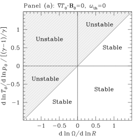
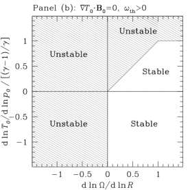
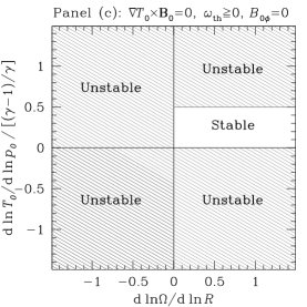
Figure 1: Stability and instability domains for rotating, barotropic [$\Omega=\Omega(R)$] fluids with isorotational unperturbed magnetic field lines (${\bf B}_{0}\cdot\nabla\Omega=0$, so $B_{0R}=0$), in the space of two parameters: angular-velocity gradient ($x$ axis) and gradient of temperature with respect to pressure ($y$ axis). Panel (a) shows the case of a plasma with isothermal unperturbed magnetic field lines ($\nabla T_{0}\cdot{\bf B}_{0}=0$, so $\partial T_{0}/\partial z=0$) in the absence of radiative cooling ($\omega_{\rm th}=0$; see Sections 4.1 and 4.2). Panel (b) shows the case of a radiatively cooling, Field-stable ($\omega_{\rm th}>0$) plasma with isothermal unperturbed magnetic field lines (see Sections 4.3 and 4.4). Panel (c) shows the case of a plasma with purely meridional unperturbed magnetic field ($B_{0\phi}=0$), with field lines orthogonal to the isothermal surfaces ($\nabla T_{0}\times{\bf B}_{0}=0$, so $\partial T_{0}/\partial R=0$), either in the absence of cooling ($\omega_{\rm th}=0$; see Section 4.1) or in the presence of cooling, but with $\omega_{\rm th}>0$ (see Section 4.3). In panels (a) and (b) ${\rm d}\ln\Omega/{\rm d}\ln R$ is normalized to $(\gamma-1)\gamma^{-1}\alpha^{-1}$, where $\alpha=2\Omega^{2}\rho_{0}{p_{0}}/|\nabla{p_{0}}|^{2}$, so the diagonal lines represent ${\rm d}\ln T_{0}/{\rm d}\ln{p_{0}}=\alpha\,{\rm d}\ln\Omega/{\rm d}\ln R$.

While in the general case of a baroclinic fluid the stability conditions (78-81) are quite involved, in the special case of a barotropic fluid the stability criterion becomes considerably simpler and can be easily shown graphically. In the barotropic case, the necessary condition $\left(\nabla T_{0}\cdot{\bf b}_{0}\right)\left(\nabla{p_{0}}\times{\bf b}_{0}\right)=0$ implies that for a configuration to be stable the magnetic field lines must be either parallel or orthogonal to the isothermal surfaces [which are also isobaric because $T_{0}=T_{0}({p_{0}})$]. Note that, when $\Omega=\Omega(R)$ the isorotation condition (17) implies that the magnetic field is vertical, so here we must assume $b_{0R}=0$.

When the unperturbed field lines are isothermal ($\nabla T_{0}\cdot{\bf b}_{0}=0$, which in the current hypotheses implies $\partial T_{0}/\partial z=\partial{p_{0}}/\partial z=\partial\Phi/\partial z=0$) the stability criterion reduces to

$$\frac{{\rm d}\ln T_{0}}{{\rm d}\ln{p_{0}}}\leq\alpha\frac{{\rm d}\ln\Omega}{{\rm d}\ln R},\qquad{\rm where}\qquad\alpha\equiv\frac{2\Omega^{2}\rho_{0}{p_{0}}}{|\nabla{p_{0}}|^{2}}$$ (85)

is a positive dimensionless factor. The corresponding domains of stability and instability are visualized in Fig. 1(a). Note that, in this special case, there can be stable configurations with ${\rm d}\Omega/{\rm d}R<0$, provided the temperature-pressure gradient is strong and negative. In the limit of uniform rotation (${\rm d}\Omega/{\rm d}R=0$) we recover the condition for stability against the MTI (see Section 3.2).

When the unperturbed field lines are parallel to the temperature gradient ($\nabla T_{0}\times{\bf b}_{0}=0$, which in the current hypotheses implies $\partial T_{0}/\partial R=\partial{p_{0}}/\partial R=0$ and $\partial\Phi/\partial R=\Omega^{2}R$) the stability conditions (78-81) reduce to

$$0\leq\frac{{\rm d}\ln T_{0}}{{\rm d}\ln{p_{0}}}\leq\frac{\gamma-1}{2\gamma}\qquad{\rm and}\qquad\frac{{\rm d}\Omega}{{\rm d}R}\geq 0,$$ (86)

which are visualized in Fig. 1(c). So, a barotropic fluid with magnetic field lines orthogonal to the isothermal surfaces is stable if and only if the angular velocity increases outwards and the temperature decreases in the direction of decreasing pressure with sufficiently shallow gradient. In other words, the condition of outward increasing angular velocity must be added to the condition for stability against the HBI found for non-rotating media (see Section 3.2). We recall that in typical astrophysical systems the angular velocity decreases outwards: the fact that the condition ${{\rm d}\Omega}/{{\rm d}R}\geq 0$ is violated is at the heart of the magnetorotational instability (MRI; Balbus & Hawley 1991, 1992), which is believed to be one of the key mechanisms at work in accretion discs.

4.2 Plasma in the absence of radiative cooling ($\omega_{\rm th}=0$) with non-vanishing azimuthal magnetic field component ($B_{0\phi}\neq 0$)

We now discuss the case in which the plasma does not cool, but the unperturbed magnetic field has a non-vanishing azimuthal component ($B_{0\phi}\neq 0$). A similar analysis was carried out by Balbus (2001), who assumed isothermal unperturbed magnetic field lines ($\nabla T_{0}\cdot{\bf b}_{0}=0$): we generalize Balbus’ result, allowing for non-isothermality of the background field lines. When $\nabla T_{0}\cdot{\bf b}_{0}\neq 0$ and $B_{0\phi}\neq 0$, but $\omega_{\rm th}=0$, the dispersion relation is

$$\begin{array}[]{c}\displaystyle n^{5}+\omega_{\rm c,a}n^{4}+\left[\omega^{2}_{\rm BV}+\omega^{2}_{\rm rot}+2\omega^{2}_{\rm A}\right]n^{3}+\left[(\omega^{2}_{\rm rot}+2\omega^{2}_{\rm A})\omega_{\rm c,a}+\omega^{2}_{\rm A}\omega_{\rm c,mag}\right]n^{2}+\\ \displaystyle\quad\,\,+\omega^{2}_{\rm A}\left(\omega^{2}_{\rm A}+\omega^{2}_{\rm BV}+\omega^{2}_{\rm rot}-4\Omega^{2}\frac{k_{z}^{2}}{k^{2}}+\omega^{2}_{\rm c,\phi}\right)n+\omega^{2}_{\rm A}\left[\left(\omega^{2}_{\rm A}+\omega^{2}_{\rm rot}-4\Omega^{2}\frac{k_{z}^{2}}{k^{2}}\right)\omega_{\rm c,a}+\omega^{2}_{\rm A}\omega_{\rm c,mag}\right]=0,\end{array}$$ (87)

which is obtained from equation (32), substituting $\omega_{\rm d}$ with $\omega_{\rm c,a}$ (because $\omega_{\rm th}=0$), and differs from equation (67) for the presence of a term proportional to $\omega_{\rm c,\phi}^{2}\propto(\nabla T_{0}\cdot{\bf b}_{0})^{2}B_{0\phi}^{2}\neq 0$. For stability, we first impose, following Appendix A, that all the Hurwitz determinants are nonnegative. We get:

$$\Delta_{2}\geq 0\iff\omega_{\rm c,a}\omega^{2}_{\rm BV}-\omega_{\rm c,mag}\omega^{2}_{\rm A}\geq 0,$$ (88)

$$\Delta_{3}\geq 0\iff\Delta_{2}\left(\omega_{\rm c,a}\omega^{2}_{\rm A}+\omega_{\rm c,mag}\omega^{2}_{\rm A}+\omega_{\rm c,a}\omega^{2}_{\rm rot}\right)-\omega^{2}_{\rm c,\phi}\omega^{2}_{\rm c,a}\omega^{2}_{\rm A}\geq 0,$$ (89)

$$\Delta_{4}\geq 0\iff\omega^{2}_{\rm A}\left[-\omega^{2}_{\rm c,a}\omega^{2}_{\rm A}\omega_{\rm c,\phi}^{4}+\left(\omega_{\rm c,mag}\omega^{2}_{\rm A}+\omega_{\rm c,a}\omega^{2}_{\rm rot}\right)\Delta_{2}\omega_{\rm c,\phi}^{2}+4\Omega^{2}{k_{z}^{2}\over k^{2}}\Delta_{2}^{2}\right]\geq 0,$$ (90)

$$\Delta_{5}\geq 0\iff\omega^{2}_{\rm A}\Delta_{4}\left[\left(\omega^{2}_{\rm A}+\omega^{2}_{\rm rot}-4\Omega^{2}{k_{z}^{2}\over k^{2}}\right)\omega_{\rm c,a}+\omega_{\rm c,mag}\omega^{2}_{\rm A}\right]\geq 0,$$ (91)

because $\Delta_{1}\geq 0$ always. Let us consider the condition $\Delta_{4}\geq 0$. This can be written in the following form:

$$-k^{2}f(x)+g(x)\geq 0,$$ (92)

where $x=k_{R}/k_{z}$ and $f(x)=\left(\omega_{\rm c,a}\omega^{2}_{\rm A}\omega^{2}_{\rm c,\phi}/k^{4}\right)^{2}\geq 0$ for all $x$. Necessary condition for the above inequality to be satisfied for all ${\bf k}$ (i.e. all $x$ and $k$) is $f(x)=0$ for all $x$. In the current hypotheses, this implies $b_{0R}=b_{0z}=0$, so ${\bf k}\cdot{\bf b}_{0}=0$ for all ${\bf k}$. However, if $b_{0R}=b_{0z}=0$ then $\omega_{\rm c,\phi}=0$, in contrast with our hypothesis, so we must conclude that there is no stable configuration with $\nabla T_{0}\cdot{\bf b}_{0}\neq 0$ and $B_{0\phi}\neq 0$.

In the case in which the unperturbed field lines are isothermal and $B_{0\phi}\neq 0$, $\omega_{\rm c,\phi}=0$ and the dispersion relation is again given by equation (67) with $\nabla T_{0}\cdot{\bf b}_{0}=0$ in $\omega_{\rm c,mag}$, which is the same as that derived, under the same hypotheses, by Balbus (2001). Analyzing this dispersion relation in the same way as in Section 4.1, we get the following stability conditions:

$$\nabla T_{0}\cdot{\bf b}_{0}=0,$$ (93)

$$-\nabla{p_{0}}\cdot\nabla\ln T_{0}+\rho_{0}\frac{\partial\Omega^{2}}{\partial\ln R}\geq 0,\qquad-\frac{\partial{p_{0}}}{\partial z}\left(\frac{\partial T_{0}}{\partial z}\frac{\partial\Omega^{2}}{\partial R}-\frac{\partial T_{0}}{\partial R}\frac{\partial\Omega^{2}}{\partial z}\right)\geq 0,$$ (94)

$$\frac{\partial{p_{0}}}{\partial z}\left(\frac{\partial\Omega^{2}}{\partial R}\frac{\partial{p_{0}}}{\partial z}-\frac{\partial\Omega^{2}}{\partial z}\frac{\partial{p_{0}}}{\partial R}\right)\geq 0,\qquad\frac{\gamma-1}{\gamma}\frac{({\bf b}_{0}\cdot\nabla{p_{0}})^{2}}{\rho_{0}{p_{0}}}+b_{0R}\left[\frac{{\bf b}_{0}\cdot\nabla(\Omega^{2}R^{4})}{R^{3}}\right]\geq 0.$$ (95)

The inequalities (94) coincide with those found by Balbus (2001), while the two conditions (95), which follow from the analysis of singular cases of the dispersion relation (67), were not reported before and, as far as we can see, are generally independent of the two conditions (94). Specializing to the case of isorotational unperturbed field lines, i.e. imposing Ferraro’s law (equation 17), the conditions (93-95) reduce to the following necessary and sufficient stability criterion:

$$\nabla T_{0}\cdot{\bf b}_{0}=0,\qquad-\nabla{p_{0}}\cdot\nabla\ln T_{0}+\rho_{0}\frac{\partial\Omega^{2}}{\partial\ln R}\geq 0,\qquad\frac{\partial{p_{0}}}{\partial z}\frac{\partial T_{0}}{\partial z}\leq 0,$$ (96)

where we have used the vorticity equation (16). In the case of a barotropic distribution with isorotational and isothermal field (so $b_{0R}={\partial{p_{0}}}/{\partial z}=0$, but $b_{0\phi}\neq 0$), the stability criterion is again condition (85), which is represented in Fig. 1(a).

4.3 Radiatively cooling plasma ($\omega_{\rm th}\neq 0$) with meridional magnetic field ($B_{0\phi}=0$)

We move now to the case in which the plasma cools radiatively ($\omega_{\rm th}\neq 0$): for simplicity we start here analyzing the dispersion relation

$$\begin{array}[]{c}\displaystyle n^{5}+\omega_{\rm d}n^{4}+\left[\omega^{2}_{\rm BV}+\omega^{2}_{\rm rot}+2\omega^{2}_{\rm A}\right]n^{3}+\left[(\omega^{2}_{\rm rot}+2\omega^{2}_{\rm A})\omega_{\rm d}+\omega^{2}_{\rm A}\omega_{\rm c,mag}\right]n^{2}+\\ \displaystyle\quad\,\,+\omega^{2}_{\rm A}\left(\omega^{2}_{\rm A}+\omega^{2}_{\rm BV}+\omega^{2}_{\rm rot}-4\Omega^{2}\frac{k_{z}^{2}}{k^{2}}\right)n+\omega^{2}_{\rm A}\left[\left(\omega^{2}_{\rm A}+\omega^{2}_{\rm rot}-4\Omega^{2}\frac{k_{z}^{2}}{k^{2}}\right)\omega_{\rm d}+\omega^{2}_{\rm A}\omega_{\rm c,mag}\right]=0,\end{array}$$ (97)

which is obtained from (32) in the hypothesis that the unperturbed magnetic field is meridional ($B_{0\phi}=0$), so $\omega_{\rm c,\phi}=0$. Performing a stability analysis as described in Appendix A, we get the following necessary conditions for stability:

$$\Delta_{1}\geq 0\iff\omega_{\rm d}\geq 0,$$ (98)

$$\Delta_{2}\geq 0\iff\omega_{\rm d}\omega^{2}_{\rm BV}-\omega_{\rm c,mag}\omega^{2}_{\rm A}\geq 0,$$ (99)

$$\Delta_{5}\geq 0\iff\left(\omega^{2}_{\rm A}+\omega^{2}_{\rm rot}-4\Omega^{2}{k_{z}^{2}\over k^{2}}\right)\omega_{\rm d}+\omega_{\rm c,mag}\omega^{2}_{\rm A}\geq 0,$$ (100)

because $\Delta_{4}$ is always nonnegative and $\Delta_{3}=\Delta_{2}\left[\omega_{\rm d}\left(\omega^{2}_{\rm A}+\omega^{2}_{\rm rot}\right)+\omega^{2}_{\rm A}\omega_{\rm c,mag}\right]\geq 0$ if $\Delta_{1}\geq 0$, $\Delta_{2}\geq 0$ and $\Delta_{5}\geq 0$. Imposing the above conditions for all wavevectors leads to the following criteria. The condition on $\Delta_{1}$ gives $\omega_{\rm th}>0$. The condition on $\Delta_{2}$ gives

$$\nabla{p_{0}}\times\nabla T_{0}=0\quad\left({\rm i.e.}\;\frac{\partial\Omega}{\partial z}=0\right),\qquad\nabla{p_{0}}\cdot\nabla{s_{0}}\leq 0,$$ (101)

$$\left(\nabla T_{0}\cdot{\bf b}_{0}\right)\left(\nabla{p_{0}}\times{\bf b}_{0}\right)=0,\qquad\nabla{p_{0}}\cdot\left[\frac{\gamma-1}{\gamma}\nabla\ln{p_{0}}-2\left(\nabla\ln T_{0}\cdot{\bf b}_{0}\right){\bf b}_{0}\right]\geq 0.$$ (102)

Exploiting the fact that we must have $\omega_{\rm th}>0$ (Field criterion) for the condition on $\Delta_{1}$, the condition on $\Delta_{5}$ gives

$$\frac{\partial\Omega}{\partial R}\geq 0,\qquad-\nabla{p_{0}}\cdot\nabla\ln T_{0}+\rho_{0}\frac{\partial\Omega^{2}}{\partial\ln R}+2(\nabla\ln T_{0}\cdot{\bf b}_{0})(\nabla{p_{0}}\cdot{\bf b}_{0})\geq 0,$$ (103)

$$-\frac{\partial{p_{0}}}{\partial z}\left[\left(\frac{\partial T_{0}}{\partial z}\frac{\partial\Omega^{2}}{\partial R}-\frac{\partial T_{0}}{\partial R}\frac{\partial\Omega^{2}}{\partial z}\right)-2\left(\nabla T_{0}\cdot{\bf b}_{0}\right)\left(b_{0z}\frac{\partial\Omega^{2}}{\partial R}-b_{0R}\frac{\partial\Omega^{2}}{\partial z}\right)\right]-\frac{\left(\nabla T_{0}\cdot{\bf b}_{0}\right)^{2}\left(\nabla{p_{0}}\times{\bf b}_{0}\right)^{2}}{R\rho_{0}T_{0}}\geq 0.$$ (104)

The singular cases to be treated separately are $\Delta_{1}=0$, $\Delta_{2}=0$, $\Delta_{3}=0$, $\Delta_{4}=0$ and $\Delta_{5}=0$, but it can be shown that they do not lead to additional conditions. In summary, taking into account that one of the conditions (101) states that the fluid must be barotropic, the necessary and sufficient stability criterion can be written as

$$\omega_{\rm th}>0,\qquad\Omega=\Omega(R),\qquad\left(\nabla T_{0}\cdot{\bf b}_{0}\right)\left(\nabla{p_{0}}\times{\bf b}_{0}\right)=0,\qquad\frac{{\rm d}\Omega}{{\rm d}R}\geq 0,\qquad\nabla{p_{0}}\cdot\nabla{s_{0}}\leq 0,$$ (105)

$$\nabla{p_{0}}\cdot\left[\frac{\gamma-1}{\gamma}\nabla\ln{p_{0}}-2\left(\nabla\ln T_{0}\cdot{\bf b}_{0}\right){\bf b}_{0}\right]\geq 0,\qquad-\nabla{p_{0}}\cdot\nabla\ln T_{0}+\rho_{0}\frac{{\rm d}\Omega^{2}}{{\rm d}\ln R}+2(\nabla\ln T_{0}\cdot{\bf b}_{0})(\nabla{p_{0}}\cdot{\bf b}_{0})\geq 0,$$ (106)

$$-\frac{\partial{p_{0}}}{\partial z}\left[\frac{\partial T_{0}}{\partial z}-2\left(\nabla T_{0}\cdot{\bf b}_{0}\right)b_{0z}\right]\geq 0.$$ (107)

The above conditions must be supplemented by the isorotation law ${\bf b}_{0}\cdot\nabla\Omega=0$, which for the relevant barotropic case implies $b_{0R}=0$ (so $b_{0z}=1$). For a barotropic fluid $T_{0}=T_{0}({p_{0}})$, so the necessary condition $\left(\nabla T_{0}\cdot{\bf b}_{0}\right)\left(\nabla{p_{0}}\times{\bf b}_{0}\right)=0$ means that for a configuration to be stable the magnetic field lines must be either parallel or orthogonal to the isothermal (and isobaric) surfaces. Let us consider first the case in which the magnetic field lines are isothermal ($\nabla T_{0}\cdot{\bf b}_{0}=0$, so $\partial T_{0}/\partial z=\partial{p_{0}}/\partial z=0$, because $b_{0R}=0$). Performing the same analysis as above, in this limit, we end up with the following necessary and sufficient stability criterion:

$$\omega_{\rm th}>0,\qquad\Omega=\Omega(R),\qquad\frac{{\rm d}\Omega}{{\rm d}R}\geq 0,\qquad\frac{{\rm d}\ln T_{0}}{{\rm d}\ln{p_{0}}}\leq\frac{\gamma-1}{\gamma},\qquad\frac{{\rm d}\ln T_{0}}{{\rm d}\ln{p_{0}}}\leq\alpha\frac{{\rm d}\ln\Omega}{{\rm d}\ln R}\qquad({\rm when}\;\nabla T_{0}\cdot{\bf b}_{0}=0),$$ (108)

where $\alpha>0$ is the dimensionless factor introduced in equation (85). These conditions are represented graphically in Fig. 1(b). When, instead, the magnetic field lines are orthogonal to the isothermal surfaces ($\nabla T_{0}\times{\bf b}_{0}=0$, so $\partial T_{0}/\partial R=\partial{p_{0}}/\partial R=0$, because $b_{0R}=0$), the stability criterion is

$$\omega_{\rm th}>0,\qquad\Omega=\Omega(R),\qquad\frac{{\rm d}\Omega}{{\rm d}R}\geq 0,\qquad 0\leq\frac{{\rm d}\ln T_{0}}{{\rm d}\ln{p_{0}}}\leq\frac{\gamma-1}{2\gamma}\qquad({\rm when}\;\nabla T_{0}\times{\bf b}_{0}=0),$$ (109)

which is visualized in Fig. 1(c).

4.4 Radiatively cooling plasma ($\omega_{\rm th}\neq 0$) with non-vanishing azimuthal magnetic field component ($B_{0\phi}\neq 0$)

We now discuss the case in which the unperturbed magnetic field has a non-vanishing azimuthal component ($B_{0\phi}\neq 0$) and the plasma is allowed to cool. This is the most general case studied in the present work, so the dispersion relation is given by equation (32), under the assumption that all terms are non-null (in particular, $\omega_{\rm th}\neq 0$ in $\omega_{\rm d}$, $\nabla T_{0}\cdot{\bf b}_{0}\neq 0$ and $B_{0\phi}\neq 0$, so $\omega_{\rm c,\phi}\neq 0$). For stability let us first impose, following Appendix A, that all the Hurwitz determinants are nonnegative. We get:

$$\Delta_{1}\geq 0\iff\omega_{\rm d}\geq 0,$$ (110)

$$\Delta_{2}\geq 0\iff\omega_{\rm d}\omega^{2}_{\rm BV}-\omega_{\rm c,mag}\omega^{2}_{\rm A}\geq 0,$$ (111)

$$\Delta_{3}\geq 0\iff\Delta_{2}\left(\omega_{\rm d}\omega^{2}_{\rm A}+\omega_{\rm c,mag}\omega^{2}_{\rm A}+\omega_{\rm d}\omega^{2}_{\rm rot}\right)-\omega^{2}_{\rm c,\phi}\omega_{\rm d}^{2}\omega^{2}_{\rm A}\geq 0,$$ (112)

$$\Delta_{4}\geq 0\iff\omega^{2}_{\rm A}\left[-\omega_{\rm d}^{2}\omega^{2}_{\rm A}\omega_{\rm c,\phi}^{4}+\left(\omega_{\rm c,mag}\omega^{2}_{\rm A}+\omega_{\rm d}\omega^{2}_{\rm rot}\right)\Delta_{2}\omega_{\rm c,\phi}^{2}+4\Omega^{2}{k_{z}^{2}\over k^{2}}\Delta_{2}^{2}\right]\geq 0,$$ (113)

$$\Delta_{5}\geq 0\iff\omega^{2}_{\rm A}\Delta_{4}\left[\left(\omega^{2}_{\rm A}+\omega^{2}_{\rm rot}-4\Omega^{2}{k_{z}^{2}\over k^{2}}\right)\omega_{\rm d}+\omega_{\rm c,mag}\omega^{2}_{\rm A}\right]\geq 0.$$ (114)

As done in Section 4.2, we note that imposing the condition $\Delta_{4}\geq 0$ for all wavevectors, in the considered case in which $b_{0\phi}\neq 0$, we get $b_{0R}=b_{0z}=0$. But if $b_{0R}=b_{0z}=0$ then $\nabla T_{0}\cdot{\bf b}_{0}=0$ and $\omega_{\rm c,\phi}=0$, in contrast with our hypothesis, so we must conclude that there is no stable configuration with $\nabla T_{0}\cdot{\bf b}_{0}\neq 0$ and $B_{0\phi}\neq 0$.

Let us thus consider the case $\nabla T_{0}\cdot{\bf b}_{0}=0$ and $B_{0\phi}\neq 0$: now $\omega_{\rm c,\phi}=0$, so the dispersion relation is equation (97) and the corresponding stability conditions are

$$\nabla T_{0}\cdot{\bf b}_{0}=0,\qquad\omega_{\rm th}>0,\qquad\frac{\partial\Omega}{\partial z}=0,\qquad\frac{\partial\Omega}{\partial R}\geq 0,$$ (115)

$$\nabla{p_{0}}\cdot\nabla{s_{0}}\leq 0,\qquad-\nabla{p_{0}}\cdot\nabla\ln T_{0}+\rho_{0}\frac{{\rm d}\Omega^{2}}{{\rm d}\ln R}\geq 0,\qquad-\frac{\partial{p_{0}}}{\partial z}\left(\frac{\partial T_{0}}{\partial z}\frac{\partial\Omega^{2}}{\partial R}-\frac{\partial T_{0}}{\partial R}\frac{\partial\Omega^{2}}{\partial z}\right)\geq 0.$$ (116)

As in Section 4.3, a necessary condition for stability is $\Omega=\Omega(R)$: note that this is a necessary requirement also in the absence of magnetic fields (see Section 3.1), but not in the absence of radiative cooling (see Sections 4.1 and 4.2). Let us focus on the case of isorotational unperturbed magnetic field lines: combining the conditions (115-116) with Ferraro’s law (equation 17) we get that the necessary and sufficient stability criterion is

$$\nabla T_{0}\cdot{\bf b}_{0}=0,\qquad\omega_{\rm th}>0,\qquad\Omega=\Omega(R),\qquad\frac{{\rm d}\Omega}{{\rm d}R}\geq 0,\qquad\frac{{\rm d}\ln T_{0}}{{\rm d}\ln{p_{0}}}\leq\frac{\gamma-1}{\gamma},\qquad\frac{{\rm d}\ln T_{0}}{{\rm d}\ln{p_{0}}}\leq\alpha\frac{{\rm d}\ln\Omega}{{\rm d}\ln R},$$ (117)

where $\alpha>0$ is the dimensionless factor introduced in equation (85). The corresponding domains of stability and instability are shown in Fig. 1(b).

5 Summary and conclusions

5.1 Magnetothermal stability criteria for rotating stratified plasmas

In the attempt to make a step forward in understanding the thermal stability of the hot atmospheres of galaxies and galaxy clusters, we have presented new stability criteria for a gravitationally stratified, rotating, radiatively cooling, weakly magnetized plasma in the presence of thermal conduction. We found that for such a medium to be stable against all linear axisymmetric disturbances it must obey several restrictive conditions, which are reported in Section 4.3 (for meridional magnetic field; equations 108-109) and Section 4.4 (for magnetic field with non-null azimuthal component; equations 115-116), and are represented in Fig. 1. Specifically, in all cases for stability the fluid is required to be Field-stable ($\omega_{\rm th}>0$), barotropic, with outward increasing angular velocity (${\rm d}\Omega/{\rm d}R\geq 0$). Additional requirements concern the relative orientation of the magnetic field lines and the thermal gradient (which must be either parallel or orthogonal) and the gradient of temperature with respect to pressure (which has different effects, depending on the relative orientation of the field lines and the thermal gradient). The above conditions can be seen as a combination and generalization of criteria for stability against the MRI (Balbus & Hawley, 1991), the MTI (Balbus, 2001), the HBI (Quataert, 2008) and the radiatively driven overstability of Balbus & Reynolds (2010). As well known, even just the two conditions $\omega_{\rm th}>0$ and ${\rm d}\Omega/{\rm d}R>0$ are typically not satisfied in standard astrophysical conditions, so we expect always to find at least one axisymmetric mode that is either monotonically unstable or overstable. Therefore, at a formal level, we must conclude that a radiatively cooling, rotating, weakly magnetized astrophysical plasma is not expected to be stable against axisymmetric perturbations. Similar conclusions were reached for magnetized (but non rotating) fluids by Balbus & Reynolds (2010) and for rotating (but unmagnetized) fluids by N10: in both cases either overstabilities or monotonic growing instabilities were expected for typical configurations. In other words, the calculations of the present paper have shown that the combination of differential rotation and a weak ordered magnetic field does not have a stabilizing effect against thermal axisymmetric perturbations.

In addition to the above results on thermal stability, we have also generalized previous studies of the stability of magnetized media in the absence of radiative cooling: in particular we have extended the study of Balbus (2001), by allowing for the presence of non-isothermal unperturbed field lines, and the study of Quataert (2008), by including the effect of differential rotation (Sections 4.1 and 4.2). The bottom line of such an analysis is that isothermality of the unperturbed field lines is a necessary requirement for stability if the magnetic field has non-vanishing azimuthal component, but, when the magnetic field is meridional, stable configurations are formally possible also with (non-isothermal) field lines orthogonal to the isobaric surfaces. In any case, the general conclusion is that, even in the absence of cooling, either overstability or monotonic instability is expected, because some of the conditions for stability are very unlikely to be satisfied in real systems (e.g., ${\rm d}\Omega/{\rm d}R\geq 0$ in the barotropic case). Formally the conditions for stability are more restrictive when cooling is effective: while in the presence of cooling the distribution must necessarily be barotropic in order to be stable, in the absence of cooling it is possible, at least in principle, to have baroclinic distributions stable against axisymmetric perturbations. However, these configurations are unlikely to be astrophysically relevant, because of the requirement of outward increasing angular velocity. Therefore it appears that radiative cooling is not the key factor determining the instability of a rotating magnetized plasma.

5.2 Implications for the hot atmospheres of galaxies and galaxy clusters

At a formal level, the above conclusions are the main results of the present work. A quite different question is what these results imply from the astrophysical point of view: in particular, what are the implications for the evolution of the hot atmospheres of galaxies and galaxy clusters? We recall that the basic underlying question is whether cool clouds can condense out of a hot, stratified medium as a consequence of the instability. To answer this question one must necessarily go beyond the formal conclusion that linear instability is expected and try to investigate the nature of the instabilities (monotonically growing or overstable), their non-linear evolution and the dependence on the properties of the perturbation. Unfortunately, we cannot address quantitatively these points based only on the presented calculations, but it is worth discussing them at least qualitatively.

As first pointed out by Malagoli et al. (1987), an important aspect of the problem is the study of the unstable modes, and, in particular, determining the nature of the instabilities: while monotonically growing instabilities are expected to naturally lead to condensation, overstable disturbances are half the time overdense and half the time underdense, with respect to the local background, so they are likely disrupted by turbulence before condensing significantly (Binney et al., 2009; Joung et al., 2012). The problem of the nature of the instabilities found in the present work could in principle be tackled analytically by studying the sign of the real roots of the dispersion relations, but, as mentioned in Appendix A, given the high order of the involved polynomials the calculations are prohibitively cumbersome (Liang & Jeffrey 2009, and references therein). Though a full exploration of the parameter space is impractical, in selected cases the question of the nature of the thermal instabilities can be addressed either by solving numerically the dispersion relations derived in this work or with magnetohydrodynamics numerical simulations, which can also be used to gain insight on the non-linear evolution of linearly unstable perturbations. For the non-rotating case, an attempt in this direction has been recently made by McCourt et al. (2012): the results of their somewhat idealized magnetohydrodynamics simulations suggest that no significant condensation occurs in the relevant regime in which the cooling time is much longer than the dynamical time.

It must be noted that all the stability criteria reported in the present work concern stability against axisymmetric perturbations. In principle, configurations that are stable against axisymmetric perturbations could be unstable when more general (non-axisymmetric) perturbations are considered. Therefore, from a mathematical point of view, exploring different kinds of disturbances could just lead to even more restrictive stability criteria. However, from the astrophysical point of view, it is clear that an axisymmetric mode is not necessarily relevant to real disturbances, and a natural question to ask is whether the instability occurs also for possibly more relevant non-axisymmetric perturbations. As well known, in the presence of differential rotation, it is considerably more complex to study non-axisymmetric than axisymmetric perturbations (e.g. Cowling, 1951; Balbus & Hawley, 1992), and such a task is beyond the purpose of the present paper. However, it is interesting to note that, at least in the unmagnetized case, non-axisymmetric perturbations tend to be stabilized by differential rotation, while this is not the case for axisymmetric disturbances (N10).

Throughout the paper we have assumed that the magnetic field is ordered over scales larger than the perturbation size. The above-presented calculations show that, if this is the case, the fluid is unlikely to stable, at least against axisymmetric disturbances. It is hard to predict the outcome of such instability, but in any case we should expect that also the structure of the magnetic field is affected. If turbulent motions are produced by the instability, the (weak) magnetic field is likely tangled by turbulence, and the system might end up in a configuration which is better described by an unmagnetized medium with suppressed isotropic thermal conductivity (Binney et al., 2009), so that the results of N10 should apply. However, it is also possible that, as a consequence of the instability, the fluid rearranges the magnetic field lines in a special ordered configuration that tends to contrast the instability, possibly leading to an overstable state (Balbus & Reynolds, 2010). In the absence of realistic non-linear calculations it appears difficult to decide which of the two above hypotheses is a better description of real systems, and of course alternative scenarios are not excluded. Overall, as far as the astrophysical implications are concerned, the results of the present work, though not allowing us to draw general conclusions on whether cool gas clouds can condense spontaneously out of an equilibrium plasma, strongly suggest that the interplay of rotation and magnetic fields is important for the thermal instability, thus encouraging further theoretical and observational investigations of the magnetic and rotational properties of the hot atmospheres of galaxies and galaxy clusters.

Appendix A Analysis of the dispersion relations: stability criteria for parametric polynomials

The dispersion relations obtained from our linear-perturbation analysis are polynomials in the complex variable $n=-{\rm i}\omega$, whose coefficients are real and generally depend on the wavevector ${\bf k}$. To obtain the linear-stability criterion we need to find the conditions under which the dispersion relation is stable for all wavevectors. From a mathematical point of view, this problem reduces to studying the stability of families of polynomials of a complex variable with real parametric coefficients.

We recall here the Routh-Hurwitz theorem, which is a fundamental tool for studying the stability of polynomials of a complex variable (e.g. Gantmacher, 1959). Let us consider an $m$-th degree polynomial

$$p(z)\equiv a_{0}z^{m}+a_{1}z^{m-1}+\cdots+a_{m};\qquad a_{0},a_{1},\ldots,a_{m}\in\mathbb{R},\qquad a_{0}\neq 0,$$ (118)

where $z\in\mathbb{C}$ and $m\geq 1$: $p(z)$ is said to be a Hurwitz polynomial, or simply a stable polynomial, if all its (generally complex) roots have negative real part. Let us associate with the polynomial $p(z)$ the following Hurwitz determinants:

$$\Delta_{j}\equiv\left|\begin{array}[]{cccccc}a_{1}&a_{3}&a_{5}&a_{7}&\cdots&a_{2j-1}\\ a_{0}&a_{2}&a_{4}&a_{6}&\cdots&a_{2j-2}\\ 0&a_{1}&a_{3}&a_{5}&\cdots&a_{2j-3}\\ 0&a_{0}&a_{2}&a_{4}&\cdots&a_{2j-4}\\ \vdots&\vdots&\vdots&\vdots&\ddots&\vdots\\ 0&0&0&0&\cdots&a_{j}\end{array}\right|,\qquad j=1,\cdots,m,$$ (119)

where it has been set $a_{i}=0$ for $i>m$. The Routh-Hurwitz theorem states that when $\Delta_{j}\neq 0$ for $j=1,\dots,m$, the polynomial $p(z)$ is stable if and only if all Hurwitz determinants are strictly positive:

$$\Delta_{1}>0,\,\Delta_{2}>0,\cdots,\,\Delta_{m}>0.$$ (120)

A corollary of the theorem is that, under the same hypotheses, a necessary condition for $p(z)$ to be stable is that all its real coefficients be strictly positive; i.e. $a_{0},a_{1},\ldots,a_{m}>0$.

It must be stressed that when at least one of the Hurwitz determinants is null the Routh-Hurwitz theorem does not apply. In our application to the dispersion relations the coefficients of the polynomial are parametric and it is not generally the case that all the Hurwitz determinants are non-null. Therefore, in order to obtain necessary and sufficient conditions for stability, we proceed as follows. We first find the conditions to have

$$\Delta_{1}\geq 0,\,\Delta_{2}\geq 0,\cdots,\,\Delta_{m}\geq 0,$$ (121)

for all wavevectors. At this stage these conditions must be considered necessary, but not sufficient, because it is not guaranteed that the singular cases ($\Delta_{i}=0$ for at least one $i$) are stable. We then consider separately the dispersion relations obtained in the singular cases, thus obtaining additional stability conditions that, combined with those obtained from (121), give the necessary and sufficient stability criterion.

When the criterion for stability is not met, one is interested in determining whether the unstable modes are monotonically growing ($z$ is real and positive) or overstable ($z$ is complex, with positive real part). Mathematically this requires a complete root classification of polynomials with real parametric coefficients. This task, which can be easily accomplished for third-order polynomials such as those considered in N10, is extremely complex for the higher-order polynomials we deal with in this work (e.g. Liang & Jeffrey, 2009). Therefore, in the present study we limit ourselves to deriving stability criteria and we do not attempt a classification of the nature of the unstable modes.

References

• Balbus (1991) Balbus S. A., 1991, ApJ, 372, 25
• Balbus (1995) Balbus S. A., 1995, ApJ, 453, 380
• Balbus (2001) Balbus S. A., 2001, ApJ, 562, 909
• Balbus & Hawley (1991) Balbus S. A., Hawley J. F., 1991, ApJ, 376, 214
• Balbus & Hawley (1992) Balbus S. A., Hawley J. F., 1992, ApJ, 400, 610
• Balbus & Reynolds (2008) Balbus S. A., Reynolds C. S., 2008, ApJ, 681, L65
• Balbus & Reynolds (2010) Balbus S. A., Reynolds C. S., 2010, ApJ, 720, L97
• Binney & Cowie (1981) Binney J., Cowie L.L., 1981, ApJ, 247, 464
• Binney et al. (2009) Binney J., Nipoti C., Fraternali F., 2009, MNRAS, 397, 1804
• Braginskii (1965) Braginskii S. I., 1965, Rev. Plasma Phys., 1, 205
• Brandenburg & Dintrans (2006) Brandenburg A., Dintrans B., 2006, A&A, 450, 437
• Brighenti et al. (2009) Brighenti F., Mathews W. G., Humphrey P. J., Buote D. A., 2009, ApJ, 705, 1672
• Carilli & Taylor (2002) Carilli C. L., Taylor G. B., 2002, ARA&A, 40, 319
• Cowling (1951) Cowling T. G., 1951, ApJ, 114, 272
• Defouw (1970) Defouw R. J., 1970, ApJ, 160, 659
• D’Ercole & Ciotti (1998) D’Ercole A., Ciotti L., 1998, ApJ, 494, 535
• Ferraro (1937) Ferraro V. C. A., 1937, MNRAS, 97, 458
• Field (1965) Field G., 1965, ApJ, 142, 531
• Fricke (1969) Fricke K., 1969, A&A, 1, 388
• Gantmacher (1959) Gantmacher F.R., 1959, The Theory of Matrices Vol.2, American Mathematical Society
• Islam (2012) Islam T., 2012, ApJ, 746, 8
• Jansson & Farrar (2012) Jansson R., Farrar G. R., 2012, ApJ, 757, 14
• Joung et al. (2012) Joung M. R., Bryan G. L., Putman M. E., 2012, ApJ, 745, 148
• Kaufmann et al. (2009) Kaufmann T., Bullock J. S., Maller A. H., Fang T., Wadsley J., 2009, MNRAS, 396, 191
• Kim & Ostriker (2000) Kim W.-T., Ostriker E. C., 2000, ApJ, 540, 372
• Kunz (2011) Kunz M. W., 2011, arXiv, arXiv:1104.3595
• Latter & Kunz (2012) Latter H. N., Kunz M. W., 2012, MNRAS, 423, 1964
• Lau, Kravtsov, & Nagai (2009) Lau E. T., Kravtsov A. V., Nagai D., 2009, ApJ, 705, 1129
• Li & Bryan (2012) Li Y., Bryan G. L., 2012, ApJ, 747, 26
• Liang & Jeffrey (2009) Liang S., Jeffrey D. J., 2009, Journal of Symbolic Computation, Volume 44, Issue 10, pages 1487-1501
• Loewenstein (1990) Loewenstein M., 1990, ApJ, 349, 471
• Malagoli et al. (1987) Malagoli A., Rosner R., Bodo G., 1987, ApJ, 319, 632
• Marinacci et al. (2011) Marinacci F., Fraternali F., Nipoti C., Binney J., Ciotti L., Londrillo P., 2011, MNRAS, 415, 1534
• Masada (2011) Masada Y., 2011, MNRAS, 411, L26
• McCourt et al. (2012) McCourt M., Sharma P., Quataert E., Parrish I. J., 2012, MNRAS, 419, 3319
• Menou, Balbus, & Spruit (2004) Menou K., Balbus S. A., Spruit H. C., 2004, ApJ, 607, 564
• Nipoti (2010) Nipoti, C. 2010, MNRAS, 406, 247 (N10)
• Parker (1953) Parker E. N., 1953, ApJ, 117, 431
• Pitts & Tayler (1985) Pitts E., Tayler R. J., 1985, MNRAS, 216, 139
• Quataert (2008) Quataert E., 2008, ApJ, 673, 758
• Salhi et al. (2012) Salhi A., Lehner T., Godeferd F., Cambon C., 2012, PhRvE, 85, 026301
• Sharma et al. (2012) Sharma P., McCourt M., Quataert E., Parrish I. J., 2012, MNRAS, 420, 3174
• Spitzer (1962) Spitzer L., 1962, Physics of Fully Ionized Gases. Wiley-Interscience, New York
• Tassoul (1978) Tassoul J.-L., 1978, Theory of Rotating Stars. Princeton University Press, Princeton
• Urpin & Brandenburg (1998) Urpin V., Brandenburg A., 1998, MNRAS, 294, 399