Scattering of electromagnetic waves by many thin cylinders: theory and computational modeling

A. G. Ramm¹ M. I. Andriychuk²

¹Mathematics Department, Kansas State University,

Manhattan, KS, 66506, USA

E-mail: ramm@math.ksu.edu

²Institute for Applied Problems in Mechanics and Mathematics, NASU,

Naukova St., 3B, 79060, Lviv, Ukraine

E-mail: andr@iapmm.lviv.ua

Abstract

Electromagnetic (EM) wave scattering by many parallel infinite cylinders is studied asymptotically as $a\to 0$, where $a$ is the radius of the cylinders. It is assumed that the centers of the cylinders $\hat{x}_{m}$ are distributed so that $\mathcal{N}(\Delta)={{\rm ln}(\frac{{1}}{{a}}}){\int\limits_{\Delta}{N(x)dx[1+o(1)]}}$, where $\mathcal{N}(\Delta)$ is the number of points $\hat{x}_{m}=(x_{m1},x_{m2})$ in an arbitrary open subset of the plane $xOy$, the axes of cylinders are parallel to $z$-axis. The function $N(x)\geq 0$ is a given continuous function. An equation for the self-consistent (limiting) field is derived as $a\to 0$. The cylinders are assumed perfectly conducting. Formula for the effective refraction coefficient of the new medium, obtained by embedding many thin cylinders into a given region, is derived. The numerical results presented demonstrate the validity of the proposed approach and its efficiency for solving the many-body scattering problems, as well as the possibility to create media with negative refraction coefficients.

Key words: EM wave scattering by many thin cylinders; asymptotic solution; refraction coefficient; effective medium theory; nanowires; computational modeling

1. Introduction

Wave scattering by many thin cylinders (nanowires) is important because of its many applications in chemistry [9], [22], medicine [23], optics [4], nanotechnology [5], etc. Analytical formulas for solving electromagnetic (EM) wave scattering problem by many thin cylinders were derived in [19], and the results from [19] are used in this paper.

There is a large literature on EM wave scattering by arrays of parallel cylinders (see, for example, [7], [8]). Our approach has the following novel features:

- the cylinders are thin, that is, they have small radius $a$, $ka\ll 1$, where $k$ is the wavenumber of the medium outside of the cylinders; this allows one to obtain a rigorous asymptotic solution of the wave scattering problem by many thin cylinders;

- the solution to the wave scattering problem is considered also in the limit $a\to 0$ when the number $M=M(a)$ of the cylinders tends to infinity at a suitable rate and the distance $d$ between neighboring cylinders is much greater than $a$, but there can be many small cylinders on the wavelength, so that the multiple scattering effects are essential; these effects are taken into account rigorously; both analytical and numerical methods for solving wave scattering problem on these thin cylinders (nanowires) are proposed and tested numerically;

- the theoretical results obtained is a basis for a method for creating a new medium with negative refraction coefficient $n^{2}(x)$; this new medium is obtained by embedding many small perfectly conducting cylinders into a given (initial) medium.

This work continues the earlier investigations in [10]-[21], and the numerical modeling presented in [1]-[3].

Let $D_{m},1\leq m\leq M$, be a set of non-intersecting domains on a plane $P$, which is $xOy$ plane. Let $\hat{x}_{m}\in D_{m},\hat{x}_{m}=(x_{m1},x_{m2})$, be a point inside $D_{m}$, $S_{m}$ be the boundary of $D_{m}$, and $C_{m}$ is the cylinder with the cross-section $D_{m}$ and the axis, parallel to $z$-axis, passing through $\hat{x}_{m}$. We assume that $\hat{x}_{m}$ is the center of the disc $D_{m}$ if $D_{m}$ is a disc of radius $a$.

Let us assume that the cylinders are perfect conductors and $a=0.5{\rm diam}D_{m}$. Our ”smallness” (thinness) assumption is

$$ka\ll 1,$$ (1)

where $k$ is the wavenumber in the region exterior to the union of the cylinders.

We assume that the thin cylinders are distributed according to the following law:

$${\mathcal{N}}(\Delta)=\ln{\frac{{1}}{{a}}}{\int\limits_{\Delta}{N(\hat{x})d\hat{x}[1+o(1)],\,\,\,\,\,\,\,a\to 0}},$$ (2)

where ${\mathcal{N}}(\Delta)={\sum\limits_{\hat{x}_{m}\in\Delta}{1}}$ is the number of the cylinders in an arbitrary open subset of the plane $P$, $N(\hat{x})\geq 0$ is a continuous function, which can be chosen as we wish. The points $\hat{x}_{m}$ are distributed in an arbitrary large but fixed bounded domain in the plane $P$. We denote by $\Omega$ the union of domains $D_{m}$, by $\Omega^{\prime}$ its complement in $P$. The complement in ${\rm R}^{{\rm 3}}$ of the union $C$ of the cylinders $C_{m}$ we denote by $C^{\prime}$.

The EM wave scattering problem consists of finding the solution to Maxwell’s equations

$$\nabla\times E=i\omega\mu H,$$ (3)

$$\nabla\times H=-i\omega\varepsilon E,$$ (4)

in $C^{\prime}$ such that

$$E_{t}=0\,\,{\rm o}{\rm n}\,\,\partial C,$$ (5)

where $\partial C$ is the union of the surfaces $C_{m}$, $E_{t}$ is the tangential component of $E$, $\mu$ and $\varepsilon$ are constants in $C^{\prime}$, $\omega$ is the frequency, $k^{2}=\omega^{2}\varepsilon\mu$. Denote by $n_{0}^{2}=\varepsilon\mu$, so $k^{2}=\omega^{2}n_{0}^{2}$.

Let us look for the solution to problem (3)-(5) of the form

$$E(x)=E_{0}(x)+v(x),\,\,x=(x_{1},x_{2},x_{3})=(x,y,z)=(\hat{x},z),$$ (6)

where $E_{0}(x)$ is the incident field, $v(x)$ is scattered field satisfying the radiation condition

$$\sqrt{r}({\frac{{\partial v}}{{\partial r}}}-ikv)=o(1),\,\,\,r=(x_{1}^{2}+x_{2}^{2})^{1/2},$$ (7)

and we assume that

$$E_{0}(x)=e^{i\kappa y+ik_{3}z}e_{1},\,\,\,\kappa^{2}+k_{3}^{2}=k^{2},$$ (8)

where $\{e_{j}\},\,j=1,2,3,$ are the unit basis vectors along the Cartesian coordinate axes $x,y,z$. We consider EM waves with $H_{3}:=H_{z}=0$, i.e., $E$-waves, or $TH$-waves,

$$E={\sum\limits_{j=1}^{3}{E_{j}e_{j}}},\,\,\,H=H_{1}e_{1}+H_{2}e_{2}={\frac{{\nabla\times E}}{{i\omega\mu}}}.$$ (9)

It is proved in [19] that the components of $E$ can be expressed by the formulas:

$$E_{j}={\frac{{ik_{3}}}{{\kappa^{2}}}}u_{x_{j}}e^{ik_{3}z},\,\,\,j=1,2,\qquad E_{3}=ue^{ik_{3}z},$$ (10)

where $u_{x_{j}}:={\frac{{\partial u}}{{\partial x_{j}}}}$; the function $u=u(x,y)$ solves the problem

$$(\Delta^{2}+\kappa^{2})u=0\,\,{\rm i}{\rm n}\,\,\Omega^{\prime},\quad\kappa^{2}:=k^{2}-k_{3}^{2},$$ (11)

$${\left.{u}\right|}_{\partial\Omega}=0,$$ (12)

$$u=e^{i\kappa y}+w,$$ (13)

and $w$ satisfies the radiation condition (7).

One can check (see [19]) that the unique solution to (11)-(13) is given by the formulas:

$$E_{1}={\frac{{ik_{3}}}{{\kappa^{2}}}}u_{x}e^{ik_{3}z},\,\,\,E_{2}={\frac{{ik_{3}}}{{\kappa^{2}}}}u_{y}e^{ik_{3}z},\,\,\,E_{3}=ue^{ik_{3}z},$$ (14)

$$H_{1}={\frac{{i\omega\varepsilon}}{{\kappa^{2}}}}u_{y}e^{ik_{3}z},\,\,\,H_{2}={\frac{{i\omega\varepsilon}}{{\kappa^{2}}}}u_{x}e^{ik_{3}z},\,\,\,H_{3}=0,$$ (15)

where $u_{x}:={\frac{{\partial u}}{{\partial x}}}$, $u_{y}$ is defined similarly, and $u=u(\hat{x})=u(x,y)$ solves scalar two-dimensional problem (11)-(13). It is proven in [12] that such a problem has a unique solution.

In [19] an asymptotic formula for this solution is derived as $a\to 0$. The results consist of the formulas for the solution to the scattering problem, of the equation for the effective field in the new medium obtained by embedding many thin perfectly conducting cylinders in the original homogeneous medium, characterized by the refraction coefficient $n_{0}^{2}$, and of a formula for the refraction coefficient in the new medium. This formula shows that by choosing a suitable distribution of thin perfectly conducting cylinders, one can change the refraction coefficient, namely, one can make it smaller than $n_{0}^{2}$, and even negative.

The paper is organized as follows.

In Section 2 we derive a linear algebraic system (LAS) for finding some numbers that define the solution to problem (11)-(13) with $M>1$, where $M$ is number of cylinders. This is a new feature of our method: instead of looking for some unknown boundary functions (currents) we look for just numbers. This method is justified only if the cylinders are thin. We also derive an integral equation for the effective (self-consistent) field in the medium with $M=M(a)$ cylinders, $M(a)\to\infty$ as $a\to 0$. At the end of Section 2 these results are applied to the problem of creating a new medium with negative refraction coefficient by embedding many thin perfectly conducting cylinders into the original (initial) medium.

In Section 3 the numerical results are presented. They demonstrate the validity and numerical efficiency of the proposed asymptotic method for solving wave scattering problems. The relative error of the solution to the LAS, to which the wave scattering problem is reduced, is investigated; the optimal parameters $M$, $a$, and $d$ that minimize the error of the asymptotic solution of the scattering problem are found. It is demonstrated numerically how the refraction coefficient of the new medium depends on the parameters $M$, $a$, and $d$.

In Section 4 the conclusions are formulated.

2. EM wave scattering by many thin cylinders

In this Section, we derive LAS for the numbers $u_{e}(\hat{x}_{j})$. These numbers determine the solution of the scattering problem by a rigorous asymptotic formula. Furthermore, we derive an integral equation for the limiting effective field, and obtain a simple explicit formula for the refraction coefficient $n^{2}$ of the new (limiting) medium.

2.1. Asymptotic formulas for the effective field

Let us assume that the domain $D$ is a union of many small domains $D_{m},\,\,D={\bigcup\limits_{m=1}^{M}{D_{m}}}$. We assume for simplicity that $D_{m}$ is a circle of radius $a$ centered at the point $\hat{x}_{m}$, and look for the solution to problem (11)-(13) of the form

$$u(\hat{x})=u_{0}(\hat{x})+{\sum\limits_{m=1}^{M}{{\int\limits_{S_{m}}{g(\hat{x},t)\sigma_{m}(t)dt}}}},$$ (16)

where $S_{m}$ is the boundary of $D_{m}$, and $dt$ is the element of the arclength of $S_{m}$.

The distribution of the points $\hat{x}_{m}$ in a bounded domain $\Omega$ on the plane $P=xOy$ is given by formula (2). The incident field is $u_{0}(\hat{x}):=e^{ikx_{2}}$, and

$$g(\hat{x},t):={\frac{{i}}{{4}}}H_{0}^{(1)}(\kappa|\hat{x}-t|).$$ (17)

The effective field acting on the $D_{j}$ is defined by the formula

$$u_{e}=u_{e}^{(j)}=u(\hat{x})-{\int\limits_{S_{j}}{g(\hat{x},t)\sigma_{j}(t)dt,\quad|\hat{x}-\hat{x}_{j}|>a}},$$ (18)

or, equivalently, by the formula

$$u_{e}(\hat{x})=u_{0}(\hat{x})+{\sum\limits_{m=1,m\neq j}^{M}{{\int\limits_{S_{m}}{g(\hat{x},t)\sigma_{m}(t)dt}}}}.$$ (19)

It is assumed that the distance $d=d(a)$ between neighboring cylinders is much greater than $a$:

$$d\gg a,\qquad{\mathop{\lim{\frac{{a}}{{d(a)}}}}\limits_{a\to 0}}=0.$$ (20)

Let us rewrite equation (16) as

$$u=u_{0}+{\sum\limits_{m=1}^{M}{g(\hat{x},\hat{x}_{m})Q_{m}}}+{\sum\limits_{m=1,m\neq j}^{M}{{\int\limits_{S_{m}}{[g(\hat{x},t)-g(\hat{x},\hat{x}_{m})]\sigma_{m}(t)dt}}}},$$ (21)

where

$$Q_{m}:={\int\limits_{S_{m}}{\sigma_{m}(t)dt}}.$$ (22)

It was proved in [19] that the second sum in (21) is negligible compared with the first one as $a\to 0$. The asymptotic formula for the numbers $Q_{m}$ is derived in [19]:

$$Q_{m}={\frac{{-2\pi u_{e}(x_{m})}}{{\ln{\frac{{1}}{{a}}}}}}[1+o(1)],\,\,a\to 0.$$ (23)

The new idea of our method consists of finding numbers $Q_{m}$ rather than unknown boundary functions $\sigma_{m}(t)$. This leads to a huge gain in the numerical efficiency of our method, and does not lead to the loss of its accuracy because $a$ is small. From formulas (21) and (23), one obtains the solution to problem (11)-(13) of the form, which is asymptotically, as $a\to 0$, exact:

$$u(\hat{x})=u_{0}(\hat{x})-{\frac{{2\pi}}{{\ln{\frac{{1}}{{a}}}}}}{\sum\limits_{m=1}^{M}{g(\hat{x},\hat{x}_{m})u_{e}(\hat{x}_{m})}}+o(1).$$ (24)

The numbers $u_{e}(\hat{x}_{m})$, $1\leq m\leq M$, in (24) are not known. Below we derive LAS (25) and (31) for finding $u_{e}(\hat{x}_{m})$. The LAS (31) is of much lower order than the LAS (25), and can be interpreted as a collocation method for solving the integral equation (30) for the self-consistent (limiting) field in the new medium. The LAS (25), on the other hand, has a clear physical meaning.

Setting $\hat{x}=\hat{x}_{j}$ in (24), neglecting $o(1)$ term, and using the definition (19) of the effective field, one gets a LAS for finding the numbers $Q_{m}$:

$$u_{e}(\hat{x}_{j})=u_{0}(\hat{x}_{j})-{\frac{{2\pi}}{{\ln{\frac{{1}}{{a}}}}}}{\sum\limits_{m=1,\,m\neq j}^{M}{g(\hat{x}_{j},\hat{x}_{m})u_{e}(\hat{x}_{m})}},\,\,\,1\leq j\leq M.$$ (25)

This system can be easily solved numerically if the number $M$ is not very large, say $M<O(10^{3})$.

2.2. Integral equation for the limiting effective field

If $M$ is very large, $M=M(a)\to\infty,\,\,a\to 0$, a linear integral equation for the limiting effective field in the new medium, obtained by embedding many thin perfectly conducting cylinders, is derived in [19].

Passing to the limit $a\to 0$ in system (25) is done as in [16]. Consider a partition of the plane domain $\Omega$, in which the small discs $D_{m}$ are distributed, into a union of $P$ small squares $\Delta_{p}$, of size $b=b(a)$, $a\ll b\ll d$. For example, one may choose $b=O(a^{1/4})$, $d=O(a^{1/2})$, so that there are many discs $D_{m}$ in the square $\Delta_{p}$. We assume that squares $\Delta_{p}$ and $\Delta_{q}$ do not have common interior points if $p\neq q$. Let $\hat{y}_{p}$ be the center of $\Delta_{p}$. One can also choose as $\hat{y}_{p}$ any point $\hat{x}_{m}$ in a domain $D_{m}\subset\Delta_{p}$. Since $u_{e}$ is a continuous function, one may approximate $u_{e}(\hat{x}_{m})$ by $u_{e}(\hat{y}_{p})$, provided that $\hat{x}_{m}\subset\Delta_{p}$.

The error of this approximation is $o(1)$ as $a\to 0$. Let us rewrite the sum in (25) as follows:

$$\frac{2\pi}{\ln(\frac{1}{a})}{\sum_{m=1,\,m\neq j}^{M}{g(\hat{x}_{j},\hat{x}_{m})u_{e}(\hat{x}_{m})}}=2\pi{\sum_{p=1,p\neq q}^{P}{g(\hat{y}_{q},\hat{y}_{p})u_{e}(\hat{y}_{p})}}{\frac{{1}}{{\ln{\frac{{1}}{{a}}}}}}\sum_{\hat{x}_{m}\in\Delta_{p}}1,$$ (26)

and use formula (2) in the form

$${\frac{{1}}{{\ln{\frac{{1}}{{a}}}}}}{\sum\limits_{\hat{x}_{m}\in\Delta_{p}}{1}}=N(y_{p})|\Delta_{p}|[1+o(1)].$$ (27)

Here $|\Delta_{p}|$ is the area of the square $\Delta_{p}$.

From (26) and (27) one obtains:

$${\frac{{2\pi}}{{\ln{\frac{{1}}{{a}}}}}}{\sum\limits_{\,m\neq j}{g(\hat{x}_{j},\hat{x}_{m})u_{e}(\hat{x}_{m})}}={\sum_{p=1,p\neq q}^{P}g(\hat{y}_{q},\hat{y}_{p})N(\hat{y}_{p})u_{e}(\hat{y}_{p})}|\Delta_{p}|[1+o(1)].$$ (28)

The sum in the right-hand side of (28) is the Riemannian sum for the integral

$${\mathop{\lim}\limits_{a\to 0}}{\sum\limits_{p=1}^{P}{g(\hat{y}_{q},\hat{y}_{p})N(\hat{y}_{p})u_{e}(\hat{y}_{p})}}|\Delta_{p}|={\int\limits_{\Omega}{g(\hat{x},\hat{y})N(\hat{y})u(\hat{y})d\hat{y}}},$$ (29)

where $u(\hat{x})={\mathop{\lim}\limits_{a\to 0}}u_{e}(\hat{x})$. Therefore, system (25) in the limit $a\to 0$ yields the following integral equation for the limiting effective (self-consistent) field $u(\hat{x})$:

$$u(\hat{x})=u_{0}(\hat{x})-2\pi{\int\limits_{\Omega}{g(\hat{x},\hat{y})N(\hat{y})u(\hat{y})d\hat{y}}}.$$ (30)

One obtains a LAS for finding unknown quantities $u(\hat{y}_{q})$, $q=1,2,.....P$, see equation (31) below, if one solves equation (30) by a collocation method with piecewise-constant basis functions. Convergence of this method to the unique solution of equation (30) is proved in [13]. Existence and uniqueness of the solution to equation (30) are proved as in [20], where a three-dimensional analog of this equation was studied.

The LAS (31) is used for the numerical calculation of the limiting effective field and for a comparison of this solution with the solution to LAS (25), whose order is much larger. The LAS is of the form:

$$u(\hat{y}_{q})=u_{0}(\hat{y}_{q})-2\pi{\sum\limits_{p=1,\,p\neq q}^{P}{g(\hat{y}_{q},\hat{y}_{p})N(\hat{y}_{p})}}u(\hat{y}_{p})|\Delta_{p}|,\,\,\,1\leq q\leq P.$$ (31)

Comparing the solution to (25) with the solution to LAS (31) one finds the range of applicability of the asymptotic formula (24) for the effective field.

2.3. The refraction coefficient for the new medium

Applying the operator $\Delta_{2}+\kappa^{2}$ to equation (30) yields the following differential equation for $u(\hat{x})$:

$$\Delta_{2}u(\hat{x})+\kappa^{2}u(\hat{x})-2\pi N(\hat{x})u(\hat{x})=0.$$ (32)

This is a Shrödinger-type equation, and $u(\hat{x})$ is the scattering solution corresponding to the incident wave $u_{0}=e^{i\kappa y}$.

If one assumes that $N(x)=N$ is a constant, then it follows from (32) that the new (limiting) medium, obtained by embedding many perfectly conducting circular cylinders, has new parameter $\kappa_{N}^{2}:=\kappa^{2}-2\pi N$. This means that $k^{2}=\kappa^{2}-k_{3}^{2}$ is replaced by $\bar{k}^{2}=k^{2}-2\pi N$. The quantity $k_{3}^{2}$ is not changed. One has $\bar{k}^{2}=\omega^{2}n^{2},\,\,k^{2}=\omega^{2}n_{0}^{2}$. Consequently, $n^{2}/n_{0}^{2}=(k^{2}-2\pi N)/k^{2}$. Therefore, the new refraction coefficient $n^{2}$ is

$$n^{2}=n_{0}^{2}(1-2\pi Nk^{-2}).$$ (33)

Since the number $N>0$ is at our disposal, equation (33) shows that choosing suitable $N$ one can create a medium with a smaller than $n_{0}^{2}$, refraction coefficient, even with negative refraction coefficient $n^{2}$.

In practice one does not go to the limit $a\to 0$, but chooses a sufficiently small $a$. As a result, one obtains a medium with a refraction coefficient $n_{a}^{2}$, which differs from (33), but the error tends to zero as $a\to 0$, and one has ${\mathop{\lim}\limits_{a\to 0}}n_{a}^{2}=n^{2}$.

3. Numerical results

Some algorithms for computational modeling of the wave scattering by many small particles were developed in [1] for the acoustic wave scattering and generalized in [2], [3] for electromagnetic (EM) wave scattering. It was proved in these papers that the asymptotic solution of the many-body wave scattering problem, proposed in [10]-[16],[20], is computationally efficient and yields accurate numerical results. On the basis of this theory a recipe for creating a material with a desired refraction coefficient was formulated. This recipe was verified numerically in [2].

In this Section, numerical results are presented. These results demonstrate the efficiency of the asymptotical approach for solving the EM wave scattering problem in the media with many embedded perfectly conducting cylinders of small radius $a$, and the possibility to create the medium with a negative refraction coefficient.

The first portion of the numerical results demonstrates the approximation errors of the numerical solutions to the LAS (25) compared to the numerical solution of LAS (31), corresponding to the collocation method for solving of the integral equation (30) for the limiting field. The rest of the numerical results demonstrate the possibility to create the media with negative refraction coefficient, and yields optimal parameters $M$, $a$, and $d$, for creating such a coefficient.

The following numerical problems are important from the practical point of view:

- to determine the values of the parameters $M$, $a$, and $d$, that provide the solution to LAS (25) with the desired accuracy, for example, with relative error of the order $10^{-3}-10^{-4})$;

- to investigate the convergence of the LAS (31) and to determine the optimal values of the parameters $M$, $a$, and $d$, which provide such convergence;

- to compare the solution to LAS (25) and LAS (31) and to find the range of $M$, $a$, and $d$ that provide accurate solutions;

- to determine the values of $M$, $a$, and $d$, which yield negative refraction coefficient.

3.1. The accuracy of the solution to LAS (25)

The numerical procedure for checking the accuracy to LAS (25) consists in calculations with various values of parameters $M$, $a$, and $d$ at $k=1.41$. First, we study the convergence of the solution depending on the number $M$ of embedded into $\Omega$ cylinders. The radius $a$ of the cylinders is changed, the distance $d$ between neighboring cylinders is kept in the range $d\geq 10a$. In Fig. 1, the relative errors of the solutions to (25) are shown for the case when number $M$ of cylinders grows from 25 to 3200. The values of $\sqrt{M}$ are depicted along the $x$ axis. Because the exact solution to (25) is not known, the relative error was calculated by formula

$${\rm R}{\rm E}={\frac{{(|u_{2M}|-|u_{M}|)}}{{|u_{2M}|}}}$$ (34)

instead of generally used

$${\rm R}{\rm E}={\frac{{(|u_{\ast}|-|u_{M}|)}}{{|u_{\ast}|}}},$$ (35)

where $u_{2M}$ and $u_{M}$ are the solution to (25) with $2M$ and $M$ cylinders respectively, $u_{\ast}$ is exact solution.

The maximal error is observed for $\sqrt{M}=5$ and it is equal to $11.2\%$. The error diminishes when $M$ grows and its value is $0.2\%$ at $M=1600$. The error practically does not depend on the radius $a$ of cylinder for big $M$. The curves presented in Fig. 2 show that absolute error has similar character and its minimal value is $0.002$ for considered $a$.

The above numerical results are obtained for $d\geq 10a$. Computationally, the values of the error depend on this ratio. This can be used for minimization of the error by choosing different $a$ and $d$. The numerical calculations show that there is an optimal value of the distance $d$ between cylinders, which provide the minimal error if $a$ is fixed. This optimal distance $d$ depends on the number $M$ of cylinders in $D$ and varies in the range $14.5a-40a$.

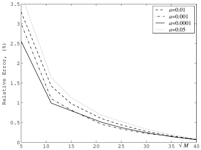
Figure 1: Relative error of solution to (25) versus $M$, $k=1.41$

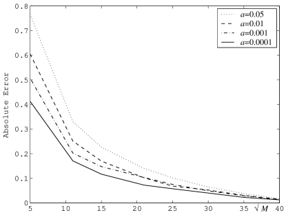
Figure 2: Absolute error of solution to (25) versus $M$, $k=1.41$

Note that the errors of $E$ components depend on the ratio of $k$ and $k_{3}$. The numerical results show that values of $\kappa$ ($\kappa^{2}=k^{2}-k_{3}^{2})$ in a neighborhood of 1 yield the minimal errors. This implies $k_{3}=1.0$ on account of $k^{2}=(1.41)^{2}=2$.

3.2. The relative error for the solution to LAS (31)

The collocation method [13] for solving LAS (31), corresponding to the limiting equation (30), is applied to check the accuracy of the numerical solution of LAS (31). The relative error is defined in the previous subsection. In Fig. 3 the dependence of the relative error on the number $P$ of the collocation points is shown. When $P$ is small, for example, $P=25$, this error is large: it is equal to $30.2\%$, $27.4\%$, and $10.4\%$ for $a=0.05$, $a=0.01$, and $a=0.001$, respectively; the error is equal to $2\%$ for $a=0.0001$. In the considered range of $P$, the error depends on $a$. The value of $ka$ does not exceed $0.0705$ here. The smallest value of $a=0.0001$ provides low error for all $P$. The values of absolute error are shown in Fig. 4. The maximal value of this error at $\sqrt{\it M}=35$ does not exceed $0.005$ and is achieved at $a=0.05$.

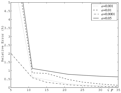
Figure 3: Relative error of solution to (31) versus $P$

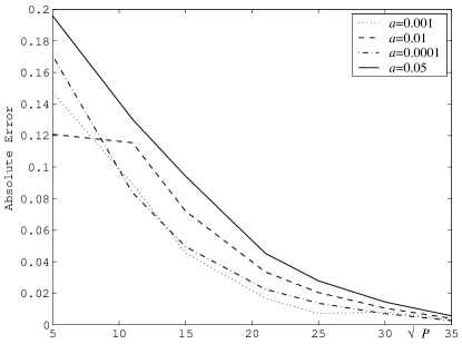
Figure 4: Absolute error of solution to (31) versus $P$

The values of the errors for the field $u$ and its $E$ components for the large $P$ at $a=0.05$ are shown in Table 1. The values of $N(x)=N$, with various constant values of $N$, are calculated by formula (2) and are shown in the last column of Table 1.

Table 1.

 

$\sqrt{P}$	Rel.Err.	Abs.Err.	Abs.Err.	Abs.Err.	Abs.Err.	$N$
	of $|u|$	of $|u|$	of $|E_{1}|$	of $|E_{2}|$	of $|E_{3}|$
40	0.76%	0.0041	0.0185	0.0205	0.0163	61.53
45	0.54%	0.0034	0.0166	0.0183	0.0147	77.89
50	0.36%	0.0028	0.0142	0.0165	0.0134	96.16
55	0.22%	0.0024	0.0126	0.0150	0.0123	116.36
60	0.10%	0.0020	0.0113	0.0139	0.0114	138.47

 

The above calculations were carried out at the values of $N$ that were determined by formula (2) for the prescribed $M$ and $d$. This implies the following formula

$$N={\frac{{{\mathcal{N}}(\Omega)}}{{\ln(1/a)|\Delta_{\Omega}|}}},$$ (36)

which agrees with formula (43) in [19] when $N(x)=N={\rm const}$, the distribution of particles is assumed in the whole $\Omega$, and $\Omega$ is the union of the non-intersecting domains $\Delta_{p}$.

In formula (36) the quantity ${\mathcal{N}}(\Omega)$ is the total number of the embedded cylinders in $\Omega$, $|\Delta_{\Omega}|$ is the area of $\Omega$, $k=1.41$. The calculations show that the value of $N(x)$, calculated by formula (36), can be varied so that it will provide the minimal error for the solution to LAS (31). In Fig. 5, the relative and absolute errors for the solution to LAS (31) are shown in a neighborhood of various values of $N$, calculated by formula (36). The first vertical line at the $x$ axis corresponds to $N=6.49$, calculated for $a=0.0001$, and the second one corresponds to $N=7.86$ for $a=0.0005$. The minimal values of the errors are to the left of the values of $N$, calculated by (36). For the considered parameters, the relative error decays from $0.72\%$ to $0.31\%$ for $a=0.0005$, and it decays from $0.64\%$ to $0.15\%$ for $a=0.0001$. The absolute error decays from $0.05$ to $0.009$ and from $0.025$ to $0.005$, respectively.

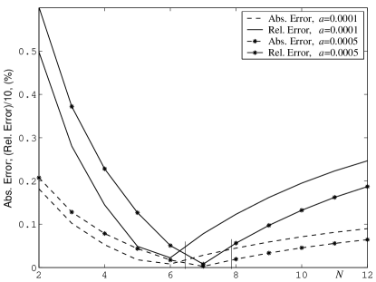
Figure 5: The absolute and relative errors of the field versus $N$

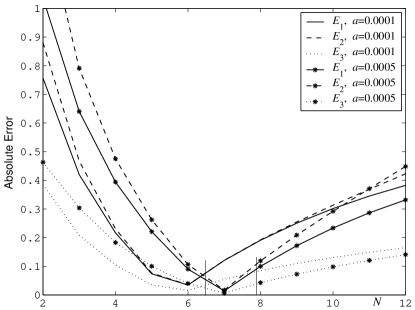
Figure 6: The absolute errors of $E$ components versus $N$

The absolute error for the $E_{j}$, $j=1,2,3,$ components of the field is presented in Fig. 6. The errors for $E_{1}$ and $E_{2}$ are higher than that for $E_{3}$ because the components $E_{1}$ and $E_{2}$ contain the derivative of function $H_{0}^{(1)}(kr)$ at the small values of $kr$, while $E_{3}$ does not contain the derivative.

The value of $N$ plays a role of an additional parameter varying which one can decrease the error. The value of $N$ can be changed by changing the distance $d$ between neighboring cylinders while keeping fixed their number in the area where $N$ is being changed.

3.3. Comparison of solutions to LAS (25) and LAS (31)

The accuracy of the asymptotic formula (24) was investigated by comparing the solutions to LAS (25) and to LAS (31). The solution to (31) with $P=4900$ collocation points is considered the benchmark solution, $k=1.41$. The relative error of this solution does not exceed $1\%$ at the considered values of $a$. This error is maximal at $a=0.05$ and it decays if $a$ decreases.

In Fig. 7 the relative and absolute errors of the solution to LAS (25) are shown at various $a$. The maximal value of the relative error is observed at $M=25$ and it is equal to $32.7\%$, $27.3\%$, and $16.6\%$ at $a=0.01$, $a=0.001$, and $a=0.0001$ respectively. This error for $\sqrt{M}=35$ is equal to $2.2\%$, $1.9\%$, and $2.4\%$.

The absolute error for $E_{1}$ and $E_{2}$ components is shown in Fig. 8. As in the preceding subsection (see Fig. 6) this error is higher than the error for $E_{3}$. The largest error for $E_{2}$ is equal to $1.2$ for $a=0.01$ when $M=25$; the minimal value of the error for this $M$ is obtained for $E_{3}$ at $a=0.0001$, and is equal to $0.13$. The minimal value of the error for $E_{3}$ component is obtained when $\sqrt{M}=35$ and this error is $0.02$.

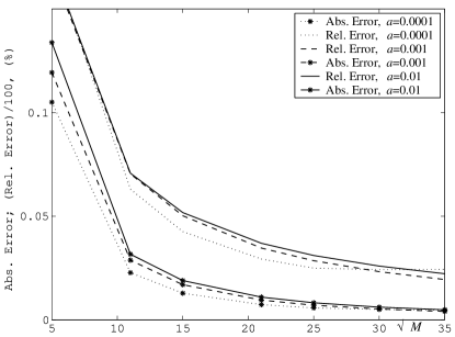
Figure 7: Absolute and relative errors of $u$ versus number $M$ of cylinders, $k=1.41$

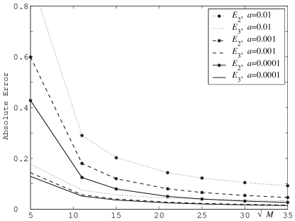
Figure 8: Absolute error of $E$ components versus number $M$ of cylinders, $k=1.41$

The above results are obtained in the case when the distance $d$ between the cylinders is fixed. It turns out that the distance parameter $d$ influences also the error of the solution to equation (24) when the number of the cylinders is fixed. The errors of the solution to equation (25) when $M=900$ for various values of $d$ are shown in Fig. 9 and Fig. 10. The benchmark solution to LAS (30) is the same as in the preceding example. There is an optimal value of $d$, which provides the minimal value of the error. The values of $na$, $n=1,2,3,....$, are shown along the $x$-axis. The minimal error equals to $0.57\%$ and is obtained when $a=0.01$ and $na=12.6$; it is equal to $0.29\%$ when $a=0.001$ and $na=16.5$, and it is equal to $0.23\%$ when $a=0.0001$ and $na=21.6$. The minimal values of absolute error when $a=0.001$ and $a=0.0001$ are shifted to the left in comparison to the minimal relative error.

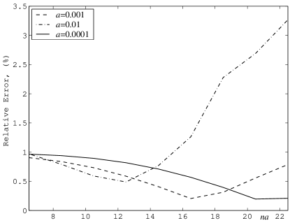
Figure 9: Relative error of $u$ versus distance $d$ between cylinders, $k=1.41$

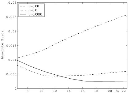
Figure 10: Absolute error of $u$ versus distance $d$ between cylinders, $k=1.41$

3.4. The refraction coefficient of the new medium

One can conclude from formula (33) that the value of the refraction coefficient $n^{2}$ depends on the wave number $k$, on the parameter $N$, on $a$, on $M$, and on $d$. In Fig. 11 and Fig. 12 the dependence of $n^{2}$ on $k$ is shown for two various values of $d$. The number $M$ of the cylinders is equal to 225. The cylinders are placed equidistantly in a square 15 cylinders on the side of the square. The lengths $l$ of square are equal to $0.1386m$ and $0.2857m$ in the Fig. 11 and Fig. 12 respectively. Consequently, the values of $d$ are equal to $0.0099m$ and $0.0204m$.

The value of $k$ has dimension $L^{-1}$, where $L$ is length, the $a$ and $d$ have dimension $L$, and the values $n^{2}$ of the refraction coefficient are normalized to the value $11.1254\cdot 10^{-18}{\frac{{{\rm s}{\rm e}{\rm k}^{2}}}{{{\rm m}^{2}}}}$. This value is obtained by multiplying $\varepsilon_{0}=8.85\times 10^{-12}F/m$ and $\mu_{0}=4\pi\times 10^{-7}H/m$, taking into account the formula $n_{0}^{2}=\varepsilon_{0}\mu_{0}$, where $F$ stands for farad, and $H$ stands for henry, $[H]=\frac{T^{2}}{F}$, $[\cdot]$ stands for the dimension of a physical quantity, and $T$ stands for time.

At the smaller $d=0.0099m$ (see Fig. 11) the values of $n^{2}$ differ considerably from the refraction coefficient $n_{0}^{2}=1$ of initial media, because more cylinders are embedded per unit area. It is seen from Fig. 12 that the refraction coefficient $n^{2}$ when $d=0.0204m$ is close to $n_{0}^{2}$. An increase of $k$ forces $n^{2}$ to get closer to initial refraction coefficient $n_{0}^{2}$. This is observed for all considered values of $a$. The considered values of the $M$, $a$, and $d$ yield the ratio $\frac{a}{d}$ less than 0.05, so condition (20) is satisfied.

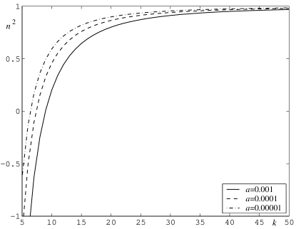
Figure 11: Values of $n^{2}$ versus wave number $k$, $M=225$, $d=0.0099m$

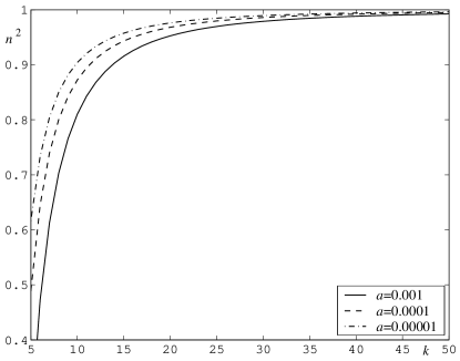
Figure 12: Values of $n^{2}$ versus wave number $k$, $M=225$, $d=0.0204m$

The numerical results presented in Fig. 13 demonstrate a possibility to create the medium with various refraction coefficients $n^{2}$ depending on the distance $d$ between the cylinders, when $a$ and $k$ are fixed. The results are shown for $a=0.0001$ and $k=20.0$. At the small values of $M$ the values of $n^{2}$ are changed considerably, and when $M$ increases $n^{2}$ tends to the following values: $n^{2}=-0.45$, $n^{2}=0.06$, $n^{2}=0.35$, and $n^{2}=0.64$ when $d=20a$, $d=25a$, $d=30a$, and $d=40a$, respectively. Note that at the considered values of the parameters the relative error of the solution to LAS (25) does not exceed $2.34\%$, $1.69\%$, $1.18\%$, and $0.93\%$ for $d=20a$, $d=25a$, $d=30a$, and $d=40a$ at $\sqrt{M}=30$, and the relative error decays when $M$ grows.

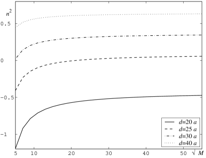
Figure 13: Values of $n^{2}$ versus the number $M$ of cylinders

Consequently, one can change the refraction coefficient $n^{2}$ by changing $k$, $a$, $M$, and $d$.

4. Conclusions

Asymptotic solution is given for the problem of EM wave scattering by many perfectly conducting parallel cylinders of small radii $a$, $ka<<1$. An equation for the effective (self-consistent) field in the limiting medium is obtained when $a\to 0$ and the distribution of the embedded cylinders is given by formula (2). The theory yields formula (33) for the refraction coefficient of the new (limiting) medium obtained by embedding of these cylinders into the initial homogeneous medium. This formula shows how the distribution of the cylinders influences the refraction coefficient.

The numerical results confirm the validity and efficiency of the asymptotic method for solving the above scattering problem. The optimal values of the parameters $k,a,d,M,N$, that minimize the error of the solution to the scattering problem, are found numerically. It is shown both theoretically and numerically that one can create negative refraction coefficients in the new medium.

References

[1] M. I. Andriychuk and A. G. Ramm. Scattering by many small particles and creating materials with a desired refraction coefficient. Intern. Journ. of Comp. Sci. and Math., Vol. 3, Nos.1/2, (2010), p. 102-121.

[2] M. I. Andriychuk, A. G. Ramm. Numerical Solution of Many-Body Wave Scattering Problem for Small Particles and Creating Materials with Desired Refraction Coefficient. In Book: Numerical Simulations of Physical and Engineering Processes. Ed. By Jan Awrejcewich, InTech, Rieka, 2011, p. 3-28.

[3] M. I. Andriychuk, S. W. Indratno, A. G. Ramm. Electromagnetic wave scattering by a small impedance particle: theory and modeling. Optics Communications, 285, (2012), p. 1684-1691.

[4] D. R. Denison, R. W. Scharstein. Decomposition of the scattering by a finite linear array into periodic and edge components. Microwave and Optical Technology Letters, Vol. 9, Issue 6, (1995), p. 338-343.

[5] S. Dubois, A. Michel, J. P. Eymery, J. L. Duvail, and L. Piraux. Fabrication and properties of arrays of superconducting nanowires. Journ. of Materials Research, 14, (1999), p. 665-671.

[6] L. Landau, E. Lifshitz. Electrodynamics of continuous media. Pergamon Press, London, 1984.

[7] P. Martin. Multiple Scattering. Cambridge Univ. Press, Cambridge, 2006.

[8] C. Mei, B. Vernescu. Homogenization methods for multiscale mechanics. Word Sci., New Jersey, 2010.

[9] S.-M. Park, G. S. W. Craig, Y.-H. La, H. H. Solak, and P. F. Nealey. Square Arrays of Vertical Cylinders of PS-$b$-PMMA on Chemically Nanopatterned Surfaces. Macromolecules, 40, (14), (2007), p. 5084-5094.

[10] A. G. Ramm. Distribution of particles which produces a ”smart” material. Journ. Stat. Phys., 127, No 5, (2007), p. 915-934.

[11] A. G. Ramm. Electromagnetic wave scattering by small bodies. Phys. Lett. A, 372/23, (2008), p. 4298-4306.

[12] A. G. Ramm. Wave scattering by many small particles embedded in a medium. Phys. Lett. A, 372/17, (2008), p. 3064-3070.

[13] A. G. Ramm. A collocation method for solving integral equations. Int. Journ. Comp. Sci. and Math., 3, No 2, (2009), p. 222-228.

[14] A. G. Ramm. A method for creating materials with a desired refraction coefficient. Intern. Journ. Mod. Phys. B, 24, (2010), p. 5261-5268.

[15] A. G. Ramm. Materials with desired refraction coefficient can be creating by embedding small particles into the given material. Intern. Journ. on Struct. Changes in Solids, 2, No 2, (2010), p. 17-23.

[16] A. G. Ramm. Wave scattering by many small bodies and creating materials with a desired refraction coefficient. Africa Matematika, 22, No 1 (2011), p. 33-55.

[17] A. G. Ramm. Electromagnetic wave scattering by a small impedance particle of arbitrary shape. Optics Communications, 284, (2011), p. 3872-3877.

[18] A. G. Ramm. Scattering of scalar waves by many small particles. AIP Advances, 1, (2011), p. 022135.

[19] A. G. Ramm. Scattering of electromagnetic waves by many thin cylinders. Results in Physics, 1, No 1, (2011), p. 13-16.

[20] A. G. Ramm. Many body wave scattering by small bodies and applications. Journ. Math. Phys., Vol. 48, No. 10, (2007), p. 103511.

[21] A. G. Ramm. Electromagnetic wave scattering by many small perfectly conducting particles of an arbitrary shape. Optics Communications, 285, (2012); http://dx.doi.org/10.1016/j.optcom.2012.05.010

[22] A. F. J. Smith and A. A. Wragg. An electrochemical study of mass transfer in free convection at vertical arrays of horizontal cylinders. Journ. of Appl. Electrochem., 4, No 3, (2009), p. 219-228.

[23] Q. Zhou and R. W. Knighton. Light scattering and form birefringence of parallel cylindrical arrays that represent cellular organelles of the retinal nerve fiber layer. Applied Optics, Vol. 36, Issue 10, (1997), p. 2273-2285.