Spin noise in quantum dot ensembles

Abstract

We study theoretically spin fluctuations of resident electrons or holes in singly charged quantum dots. The effects of external magnetic field and effective fields caused by the interaction of electron and nuclei spins are analyzed. The fluctuations of spin Faraday, Kerr and ellipticity signals revealing the spin noise of resident charge carriers are calculated for the continuous wave probing at the singlet trion resonance.

I Introduction

Spin noise technique has recently become one of the most promising methods to study electron spin dynamics in various material systems,Mueller2010 including atomic gases Crooker_Noise and semicoductors.Oestreich_noise ; muller:206601 ; PhysRevB.79.035208 ; crooker2010 ; dahbashi2012 ; crooker2012 This technique first implemented in Ref. aleksandrov81, to observe the magnetic resonance of the sodium atoms is based on the monitoring of spin fluctuations by means of spin Faraday or Kerr rotation effect for the linearly polarized continuous wave (cw) probe. Namely, the spin Faraday ($\vartheta_{\mathcal{F}}$) or Kerr ($\vartheta_{\mathcal{K}}$) rotation angles are proportional to the vector component $S_{z}$ of the instant magnetization of the medium onto the radiation propagation direction $z$. Hence, the angle fluctuations reveal the spin autocorrelations

$$\langle\vartheta_{\mathcal{F}}(t)\vartheta_{\mathcal{F}}(t^{\prime})\rangle,\ \langle\vartheta_{\mathcal{K}}(t)\vartheta_{\mathcal{K}}(t^{\prime})\rangle\propto\langle S_{z}(t)S_{z}(t^{\prime})\rangle\>,$$ (1)

where the angle brackets mean averaging over the time $t$ for a fixed value of the difference $t^{\prime}-t$. The average $\langle S_{z}(t)S_{z}(t^{\prime})\rangle$ characterizes the magnitude of electron spin fluctuations and contains an important information about the spin relaxation and decoherence processes. The spin noise technique is especially well suited to study slow spin relaxation in semiconductor nanostructures.Mueller2010 ; dahbashi2012 ; crooker2012 ; sherman

Contemporary studies of the spin noise in the quantum dot ensembles made it possible to extract electron and hole Landé factors and decoherence rates.crooker2010 ; dahbashi2012 Such systems are highly perspective for the future spintronics applications due to a number of fascinating phenomena, e.g., spin precession mode-locking where a macroscopic number of spins can precess synchronously under the conditions of pulse-train optical excitation.A.Greilich07212006 ; A.Greilich09282007 Electron spin dynamics in quantum dot ensembles is being extensively studied, see the review articles [yakovlev_bayer, ], [glazov:review, ] and references therein, while the microscopic theory of the spin noise in these systems is absent to the best of our knowledge. The present paper is aimed to fill the gap.

Here we address theoretically spin fluctuations of electrons and holes in quantum dot ensembles. The effects of external magnetic field as well as the role of hyperfine coupling of carrier spins with nuclei are discussed in detail. The features of the spin noise spectra related to the system inhomogeneity are of special attention. Finally, we derive microscopic expressions for the fluctuation spectra of spin Faraday, Kerr and ellipticity effects for quantum dot ensembles and perform comparative analysis of these spectra.

II Model

The spin fluctuation $\delta{\bm{s}}(t)$ can be described by the Langevin method applied to the Bloch equation as follows

$$\frac{\partial\delta{\bm{s}}(t)}{\partial t}+\frac{\delta{\bm{s}}(t)}{\tau_{s}}+\delta{\bm{s}}(t)\times\left({\bm{\Omega}}_{\bm{B}}+{\bm{\Omega}}_{N}\right)={\bm{\xi}}(t)\>.$$ (2)

Here $\tau_{s}$ is the electron spin relaxation time caused by, e.g., electron-phonon interaction, PhysRevB.64.125316 ; PhysRevB.66.161318 ${\bm{\Omega}}_{\bm{B}}$ and ${\bm{\Omega}}_{N}$ are the Larmor precession frequencies related to the external magnetic field ${\bm{B}}$ and the effective field caused by the hyperfine electron-nuclear interaction, ${\bm{\xi}}(t)$ is the fictitious random force. For simplicity, we assume an isotropic symmetry of the spin system characterized by single spin-relaxation time and electron $g$-factor. The hyperfine interaction of electron and nuclei spins in the quantum dot results in the effective magnetic field acting on electron spin. This field is induced by the nuclear spin fluctuations and differs from dot to dot, giving rise to the electron spin dephasing.kkm_nucl_book ; merkulov02 ; PhysRevLett.88.186802 On the timescale of electron spin precession in the hyperfine field induced by the nuclear spin fluctuation, the latter can be considered as static.merkulov02 ; yugova11 The magnetic field is assumed to be weak enough in order not to affect the spin relaxation time $\tau_{s}$ and nuclear spin fluctuations. Then the correlator of the Langevin force coincides with that for the equilibrium spin decoupled from the magnetic field ${\bm{B}}$ and the nuclei, namely,

$$\langle\xi_{\alpha}(t^{\prime})\xi_{\beta}(t)\rangle=\frac{1}{2\tau_{s}}\delta_{\alpha\beta}\delta(t^{\prime}-t)\>,$$ (3)

where $\alpha,\beta=x,y$ and $z$ are the Cartesian coordinates. This equation can readily be derived by using the Langevin approach in the general fluctuation theory ggk ; LandauStat applied to a physical variable $x$, e.g., the velocity or spin of a particle, describing by $\dot{x}(t)+x(t)/\tau_{0}=0$ the time decay of its nonequilibrium average value. In this approach the equilibrium fluctuation $\delta x(t)$ satisfies the one-dimensional equation of random motion $\delta\dot{x}(t)+\delta x(t)/\tau_{0}=\xi(t)$ with the inhomogeneous term $\xi(t)$ called the Langevin force. The correlator of $\xi(t)$ is connected with the dispersion $\langle\delta x^{2}\rangle$ by LandauStat

$$\langle\xi(t^{\prime})\xi(t)\rangle=(2/\tau_{0})\langle\delta x^{2}\rangle\delta(t^{\prime}-t)\>.$$

Equation (3) follows from this general equation if we take into account that, for the spin $s=1/2$, the spin-component dispersion $\langle s_{\alpha}^{2}\rangle=1/4$. We stress that the fictitious random force $\bm{\xi}(t)$ is not related with any real physical processes, it is introduced in Eq. (2) in the Langevin approach to provide the proper values of the spin fluctuations in equilibrium. This approach is known as a convenient and effective description of fluctuations.ggk ; lax2

The spectral decomposition of fluctuations is based on the standard Fourier transforms of the fluctuating spin,

$$\delta{\bm{s}}_{\omega}=\int\limits_{-\infty}^{+\infty}\delta{\bm{s}}(t){\rm e}^{{\rm i}\omega t}dt\>,\>\delta{\bm{s}}(t)=\int\limits_{-\infty}^{+\infty}\delta{\bm{s}}_{\omega}{\rm e}^{-{\rm i}\omega t}\frac{d\omega}{2\pi}\>,$$

and the spin and random-force correlators

$$(\delta s_{\alpha}\delta s_{\beta})_{\omega}=\int\limits_{-\infty}^{+\infty}\langle\delta s_{\alpha}(t+\tau)\delta s_{\beta}(t)\rangle{\rm e}^{{\rm i}\omega\tau}d\tau\>,$$ (4)

$$(\xi_{\alpha}\xi_{\beta})_{\omega}=\int\limits_{-\infty}^{+\infty}\langle\xi_{\alpha}(t+\tau)\xi_{\beta}(t)\rangle{\rm e}^{{\rm i}\omega\tau}d\tau=\frac{1}{2\tau_{s}}\delta_{\alpha\beta}\>.$$

The Fourier component $\delta{\bm{s}}_{\omega}$ satisfies the vector equation obtained from Eq. (2) by the replacements $\partial/\partial t\to-{\rm i}\omega$, $\delta{\bm{s}}(t)\to\delta{\bm{s}}_{\omega}$ and ${\bm{\xi}}(t)\to{\bm{\xi}}_{\omega}$. According to Eq. (3) the double correlator of the random-force Fourier transforms is given by

$$\langle\xi_{\alpha,\omega}\xi_{\beta,\omega^{\prime}}^{*}\rangle=\delta(\omega-\omega^{\prime})\delta_{\alpha\beta}\frac{\pi}{\tau_{s}}\>.$$

The solution of Eq. (2) for the spin pseudovector reads

$$\delta{\bm{s}}_{\omega}=\tau_{s,\omega}\frac{{\bm{\xi}}_{\omega}+\tau_{s,\omega}{\bm{\Omega}}\times{\bm{\xi}}_{\omega}+\tau_{s,\omega}^{2}{\bm{\Omega}}({\bm{\xi}}_{\omega}\cdot{\bm{\Omega}})}{1+{\bm{\Omega}}^{2}\tau^{2}_{s,\omega}}\>,$$ (5)

where

$${\bm{\Omega}}={\bm{\Omega}}_{\bm{B}}+{\bm{\Omega}}_{N}\hskip 5.69054pt\mbox{and}\hskip 5.69054pt\tau_{s,\omega}=\frac{\tau_{s}}{1-\mathrm{i}\omega\tau_{s}}\>.$$ (6)

The relation (5) between the spin ${\bm{s}}_{\omega}$ and the random force ${\bm{\xi}}_{\omega}$ can formally be obtained from the equation (9) in Ref. merkulov, relating the average spin $\bar{\bm{s}}$ and the initial spin ${\bm{s}}_{0}$ by replacing $\bar{\bm{s}}$ to ${\bm{s}}_{\omega}$, $\tau_{c}$ to $\tau_{s,\omega}$, and ${\bm{s}}_{0}$ to $\tau_{s,\omega}{\bm{\xi}}_{\omega}$. By introducing the linear-response tensor ${\bm{\chi}}(\omega)$ defined as

$$\delta s_{\alpha,\omega}=\chi_{\alpha\beta}(\omega)\xi_{\beta,\omega}\>,$$ (7)

we can present the spin-fluctuation spectrum in the form

$$(\delta s_{\alpha}\delta s_{\beta})_{\omega} = \frac{1}{2\tau_{s}}\sum\limits_{\gamma}\chi_{\alpha\gamma}(\omega)\chi^{*}_{\beta\gamma}(\omega)$$ (8)

$$= \frac{1}{2\tau_{s}}\left[{\bm{\chi}}(\omega){\bm{\chi}}^{{\dagger}}(\omega)\right]_{\alpha\beta}\>.$$

The components of the tensor ${\bm{\chi}}(\omega)$ are explicitly given by

$$\chi_{\alpha\beta}(\omega)=\frac{\tau_{s,\omega}\left(\delta_{\alpha\beta}-\delta_{\alpha\beta\gamma}\Omega_{\gamma}\tau_{s,\omega}+\tau_{s,\omega}^{2}\Omega_{\alpha}\Omega_{\beta}\right)}{1+{\bm{\Omega}}^{2}\tau^{2}_{s,\omega}}\>,$$ (9)

where $\delta_{\alpha\beta\gamma}$ is the unit antisymmetric third-rank tensor. Equation (8) can also be derived by means of the fluctuation-dissipation theorem, see Appendix for details, or from kinetic equations for the spin-spin correlation functions $\langle\delta s_{\alpha}(t)\delta s_{\beta}(t^{\prime})\rangle$ similar to the general approach of Ref. LandauKin, . To summarize, Eqs. (8) and (9) are valid provided: (i) $\tau_{s}$ is magnetic field independent, (ii) nuclear field $\bm{\Omega}_{N}$ is static (or quasistatic).

Let us consider the simple limiting cases to show that Eq. (8) readily describes them. In the absence of external and internal fields, $\bm{\Omega}=0$, the response reduces to $\chi_{\alpha\beta}(\omega)=\tau_{s,\omega}\delta_{\alpha\beta}$ and we have

$$(\delta s_{\alpha}\delta s_{\beta})_{\omega}=\frac{|\tau_{s,\omega}|^{2}}{2\tau_{s}}\delta_{\alpha\beta}=\frac{1}{2}\frac{\tau_{s}}{1+(\omega\tau_{s})^{2}}\delta_{\alpha\beta}\>,$$ (10)

in agreement with Refs. Mueller2010, , ivchenko73fluct_eng, . For a system subjected to an external magnetic field ${\bm{B}}$ but free from the hyperfine interaction, it is convenient to use the Cartesian coordinate frame $1,2,3$ with the axis $3\parallel{\bm{\Omega}}_{\bm{B}}$. In this case

$$||\chi_{\alpha\beta}(\omega)||=\frac{\tau_{s,\omega}}{1+(\Omega_{3}\tau_{s,\omega})^{2}}\hskip 28.45274pt$$ (11)

$$\times\left[\begin{array}[]{ccc}1&-\Omega_{3}\tau_{s,\omega}&0\\ \Omega_{3}\tau_{s,\omega}&1&0\\ 0&0&1+(\Omega_{3}\tau_{s,\omega})^{2}\end{array}\right]\>.$$ (15)

Substitution of this tensor into Eq. (8) leads to the following nonzero components of the tensor $(\delta s_{\alpha}\delta s_{\beta})_{\omega}$:

$$(\delta s_{3}^{2})_{\omega}=\frac{\pi}{2}\Delta(\omega)\>,$$ (16)

$$(\delta s_{1}^{2})_{\omega}=(\delta s_{2}^{2})_{\omega}=\frac{\pi}{4}[\Delta(\omega-\Omega_{3})+\Delta(\omega+\Omega_{3})]\>,$$

$$(\delta s_{2}\delta s_{1})_{\omega}=(\delta s_{1}\delta s_{2})^{*}_{\omega}=\frac{2{\rm i}\omega\Omega_{3}\tau_{s}^{2}}{1+\tau^{2}_{s}(\omega^{2}+\Omega_{3}^{2})}(\delta s_{1}^{2})_{\omega}\>,$$

where

$$\Delta(x)=\frac{1}{\pi}\frac{\tau_{s}}{1+(x\tau_{s})^{2}}\>.$$

Equations (16) are also valid in the absence of an external magnetic field but in the presence of a fixed hyperfine field, in this case $3\parallel\bm{\Omega}_{N}$.

III Spin fluctuations in quantum-dot ensembles

Until now, we described electron spin fluctuations in a single dot. In a quantum-dot ensemble the spin noise spectrum per quantum dot is obtained by averaging Eq. (8) over the direction and absolute value of ${\bm{\Omega}}_{N}$

$$(\delta s_{\alpha}\delta s_{\beta})_{\omega}=\frac{1}{2\tau_{s}}\int d{\bm{\Omega}}_{N}{\cal F}({\bm{\Omega}}_{N})\left[{\bm{\chi}}(\omega){\bm{\chi}}^{{\dagger}}(\omega)\right]_{\alpha\beta}\>,$$ (17)

where ${\cal F}({\bm{\Omega}}_{N})$ is the distribution function of the nuclear fields acting on electron spins in the quantum dot ensemble. Due to the $s$-type character of the conduction band Bloch functions the hyperfine interaction strength is proportional to the scalar product of electron and nuclear spins, resulting in an isotropic distribution of the nuclei-induced electron spin precession frequencies ${\bm{\Omega}}_{N}$. Therefore $\mathcal{F}({\bm{\Omega}}_{N})$ depends only on the absolute value of the nuclear field.

III.1 Spin fluctuations in the absence of external field

At zero magnetic field, the averaging over the direction results in the simplification of $(\delta s_{\alpha}\delta s_{\beta})_{\omega}$ to $\delta_{\alpha\beta}(\delta s_{\alpha}^{2})_{\omega}$ with $(\delta s_{\alpha}^{2})_{\omega}=[(\delta s_{1}^{2})_{\omega}+(\delta s_{2}^{2})_{\omega}+(\delta s_{3}^{2})_{\omega}]/3$ and, therefore,

$$(\delta s_{\alpha}^{2})_{\omega}=\frac{\pi}{6}\left\{\Delta(\omega)\right.\hskip 56.9055pt$$ (18)

$$+\int_{0}^{\infty}d\Omega_{N}\ F(\Omega_{N})\ [\Delta(\omega-\Omega_{N})+\Delta(\omega+\Omega_{N})]\}\>,$$

where

$$F(\Omega_{N})=4\pi\Omega_{N}^{2}\mathcal{F}(\Omega_{N})$$

is the distribution of absolute values of the hyperfine fields. The factor $4\pi\Omega_{N}^{2}$ takes into account a three-dimensional character of the random vector $\bm{\Omega}_{N}$. Equation (18) clearly shows that the spin noise spectrum contains two contributions. First one is centered at $\omega=0$ and stems from fluctuations of the spin component directed along the nuclear field which is considered as static here. In that way the zero-frequency peak bears information about the single-electron spin relaxation time $\tau_{s}$. Note, that for sufficiently long spin relaxation times the electron hyperfine interaction with nuclei may modify slow electron spin dynamics and, correspondingly, the low frequency spin noise spectra, due to coupled spin dynamics of electrons and nuclei.coupled1 The second contribution to the spin noise spectrum reflects electron spin precession in random nuclei-induced fields. Provided that $\Omega_{N}\tau_{s}\gg 1$ this contribution to the spin noise spectrum, for $\omega>0$, reduces to $(\pi/6)F(\omega)$ and describes the distribution of the nuclear-induced spin precession fluctuations.

The electron spin noise spectrum calculated for the quantum dot ensemble is shown in Fig. 1(a) for the Gaussian distribution of nuclear fields acting on the electron spin, $\mathcal{F}(\bm{\Omega}_{N})=(\sqrt{\pi}\delta_{e})^{-3}\exp{(-\Omega_{N}^{2}/\delta_{e}^{2})}$, where $\delta_{e}$ describes the dispersion of the nuclear field fluctuation.merkulov02 ; chemphys Two contributions to the spin noise spectrum are clearly seen: the narrow peak at $\omega=0$, which is well described by $\Delta(\omega)$, and much wider peak at $\omega=\delta_{e}$ corresponding to the distribution of nuclear fields $(\pi/6)F(\omega)$. The Fourier transform of Eq. (18) to the time domain gives the relaxation dynamics of the spin component $s_{\alpha}$; for the Gaussian distribution of nuclear spins and in the limit $\tau_{s}\to\infty$, it reduces to Eq. (10) of Ref. merkulov02, , see also Ref. zhang06, .

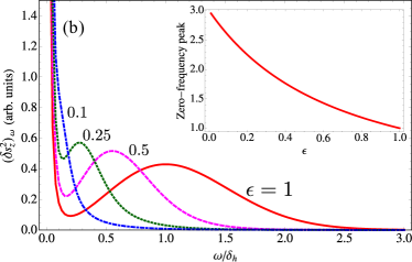
Figure 1: (a) Spin noise spectrum for electrons (red solid curve) and its decomposition into the zero frequency peak (dotted) and the peak corresponding to nuclei-induced precession (dashed) calculated for $\delta_{e}\tau_{s}=100$. Inset shows the spin noise spectrum in the double logarithmic scale. (b) Heavy-hole pseudospin noise spectrum calculated for different values of anisotropy parameter $\epsilon$ (marked at each curve). Inset shows the amplitude of zero-frequency peak (normalized to its value at $\epsilon=1$) as a function of the anisotropy parameter calculated for $\delta_{h}\tau_{s}=100$.

Next we turn to the spin fluctuations of holes in quantum dots. Here, for distinctness, we consider heavy-hole states, namely, the doubly-degenerate hole states with the angular momentum projection $J_{z}=\pm 3/2$ onto the growth axis of the quantum dot. Occupation of this pair of states can be described by means of the pseudospin-$1/2$ three-component vector $\tilde{\bm{s}}$. Contrary to electrons, the coupling of a heavy hole and nuclear spins results not from the contact hyperfine interaction but rather from the relatively weak dipole-dipole interaction. The latter is strongly anisotropic in quantum dots. In particular, if the mixing of heavy-hole ($\pm 3/2$) and light-hole ($\pm 1/2$) states and contributions related with the cubic symmetry of the crystalline lattice are disregarded, the effective magnetic field experienced by the hole spin is parallel to the $z$ axis and proportional to the nuclear spin $z$ component.perel76eng ; PhysRevB.78.155329 ; PhysRevB.79.195440 In real quantum-dot structures heavy holes additionally experience an effective field of the in-plane nuclear-spin components PhysRevLett.102.146601 which is, however, weaker than that caused by the $z$ component. As a result, we model the distribution of effective fields acting on the hole spins by an anisotropic Gaussian function:

$$\mathcal{F}_{h}(\bm{\Omega})=\frac{1}{\pi^{3/2}\delta_{h}^{3}\epsilon^{2}}\exp{\left(-\frac{\Omega_{z}^{2}}{\delta_{h}^{2}}-\frac{\Omega_{\perp}^{2}}{(\epsilon\delta_{h})^{2}}\right)}\>,$$ (19)

where $\bm{\Omega}_{\perp}=(\Omega_{x},\Omega_{y})$ is the in-plane component of the effective Larmor frequency, a value of $\epsilon$ lies in the interval between 0 and 1 and characterizes the relative strength of the hole coupling with the in-plane nuclear fields, and an in-plane anisotropy of hole-nuclear coupling is neglected. Fluctuations of the $z$-component of hole pseudospin are given by

$$(\delta\tilde{s}_{z}^{2})_{\omega}=\frac{\pi}{2}\int d\bm{\Omega}\ \mathcal{F}_{h}(\bm{\Omega})\\ \times\left\{\frac{\Omega_{z}^{2}}{\Omega^{2}}\ \Delta(\omega)+\frac{\Omega_{\perp}^{2}}{\Omega^{2}}\ \biggl{[}\Delta(\omega-\Omega)+\Delta(\omega+\Omega)\biggr{]}\right\}\>,$$ (20)

where $\bm{\Omega}=(\Omega_{x},\Omega_{y},\Omega_{z})$ and $\Omega^{2}=\Omega_{\perp}^{2}+\Omega_{z}^{2}$.

Figure 1(b) shows the heavy-hole pseudospin noise spectrum calculated for different values of the anisotropy parameter $\epsilon$. The fluctuation spectrum is similar to that for electrons, see curve corresponding to $\epsilon=1$ and Fig. 1(a), and contains two peaks: at zero frequency, due to the first term in Eq. (20), and the high-frequency peak described by the second term in the curly brackets of Eq. (20). Note that for $\epsilon<1$ the height of the zero-frequency peak is enhanced as compared with that for electrons, see inset in Fig. 1(b). In the limit of strong anisotropy $\epsilon\ll 1$ it is three times higher than in the isotropic case, since, for $\epsilon\to 0$, the effective nuclear field is always directed along $z$ axis. The high-frequency peak shifts towards the zero frequency with decreasing $\epsilon$ and eventually merges with the zero-frequency peak. Note, that while comparing quantitatively with experiments one has to allow for the hole spin relaxation anisotropy and introduce the longitudinal and transverse relaxation times.

III.2 Spin fluctuations in the external magnetic field

In the presence of an external magnetic field the electron (hole) spin precession frequency $\bm{\Omega}$ has, according to Eq. (6), two contributions due to (i) interaction with nuclei $\bm{\Omega}_{N}$ and (ii) interaction with an external field, $\bm{\Omega}_{\bm{B}}$. Making use of Eq. (17) we recast the spectrum of the spin $z$ component fluctuations in the following form [cf. Eq. (20)]

$$(\delta s^{2}_{z})_{\omega}=\frac{\tau_{s}}{2}\int d{\bm{\Omega}}_{N}\ \mathcal{F}({\bm{\Omega}}_{N})\times$$ (21)

$$\left\{\sin^{2}{\theta}\frac{1+(\omega^{2}+\Omega^{2})\tau_{s}^{2}}{[1+(\omega-\Omega)^{2}\tau_{s}^{2}][1+(\omega+\Omega)^{2}\tau_{s}^{2}]}+\frac{\cos^{2}{\theta}}{1+\omega^{2}\tau_{s}^{2}}\right\}.$$

where $\theta$ is the angle between the vector ${\bm{\Omega}}={\bm{\Omega}}_{N}+{\bm{\Omega}}_{\bm{B}}$ and $z$ axis and $\Omega=|{\bm{\Omega}}_{\bm{B}}+{\bm{\Omega}}_{N}|$. In the absence of the nuclear spin fluctuations Eq. (21) reduces (up to a common factor) to Eq. (5) of Ref. braun, .

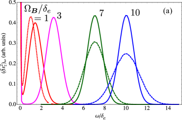
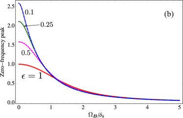
Figure 2: (a) Spin noise spectrum for electrons in the transverse magnetic field (solid) for $\delta_{e}\tau_{s}=100$. Ratio between $\Omega_{\bm{B}}$ and $\delta_{e}$ is indicated at each curve. Red dotted curve shows electron spin noise spectrum at $\bm{B}=0$ [c.f. red curve in Fig. 1(a)], dashed green and blue curves demonstrate spin noise spectra calculated with a $10$% spread of electron $g$-factor. (b) Zero-frequency peak amplitude (normalized to its value at $\bm{B}=0$, $\epsilon=1$) calculated as a function of the magnetic field for $p$-type quantum dot ensemble. Different curves correspond to different values of the anisotropy parameter $\epsilon$ (marked at each curve).

Figure 2(a) shows the electron spin noise spectrum in the transverse magnetic field $\bm{\Omega}_{\bm{B}}\perp z$. Such a case corresponds to the most widespread experimental configuration of the spin noise measurements. Mueller2010 Calculation shows that the noise peak at $\omega\neq 0$ shifts proportionally to $\Omega_{\bm{B}}$ for sufficiently high magnetic fields ($\Omega_{\bm{B}}\gg\delta_{e}$) and its height slightly increases with an increase of magnetic field. In such a case, the spin fluctuation dispersion is controlled only by the parallel to $\bm{\Omega}_{\bm{B}}$ component of the nuclear spin fluctuations and, at $\delta_{e}\tau_{s}\gg 1$, the spin noise spectrum can be reduced to

$$(\delta s_{z}^{2})_{\omega}=\frac{\pi}{8}\int\limits_{0}^{\infty}\frac{F\left[\sqrt{\Omega_{N}^{2}+(\omega-\Omega_{\bm{B}})^{2}}\right]\Omega_{N}d\Omega_{N}}{\Omega_{N}^{2}+(\omega-\Omega_{\bm{B}})^{2}}\,.$$ (22)

With the further increase in magnetic field, the spin noise spectrum is additionally affected by the inhomogeneous broadening of electron $g$-factor values similarly to the spin dephasing of the localized carriers.yakovlev_bayer This effect is illustrated by the dashed curves in Fig. 2(a) where a $10$% spread of electron $g$-factor values was additionally considered. The $g$-factor dispersion is modeled by the Gaussian distribution, see Ref. glazov08a, for details. The spin noise spectra of quantum dots with resident holes have a similar shape.

The transverse magnetic field affects also the zero-frequency peak. Figure 2(b) demonstrates the magnitude of the zero-frequency peak as a function of magnetic field calculated for the case of the positively charged quantum dot ensemble. Different curves correspond to different values of anisotropy parameter $\epsilon$. Figure shows that the magnetic field suppresses the zero-frequency peak, because the higher the field, the smaller the probability to find the quantum dot with $\bm{\Omega}=\bm{\Omega}_{N}+\bm{\Omega}_{\bm{B}}\parallel z$. In other words, the average value of $\cos^{2}{\theta}$ in Eq. (21) decreases with an increase in the transverse magnetic field.

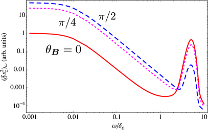
Figure 3: Spin noise spectrum for electrons in the magnetic field $\bm{B}$ applied at the angle $\theta_{\bm{B}}=0$ (red solid), $\pi/4$ (magenta dotted) and $\pi/2$ (blue dashed) to the $(xy)$ plane. Electron $g$-factor is assumed to be isotropic, $\Omega_{\bm{B}}/\delta_{e}=5$, $\delta_{e}\tau_{s}=100$.

The situation is different if the applied magnetic field acquires a longitudinal (parallel to $z$-axis) component. The spin noise spectra are presented in Fig. 3. It is clearly seen that the peak corresponding to the non-zero frequency becomes suppressed with the increasing of the tilt angle of magnetic field with respect to the quantum dot plane, while the zero-frequency peak becomes higher. Indeed, the considerable $z$ component of the external magnetic field leads to the diminishing of the transversal nuclear field role resulting in an enhancement of the zero-frequency peak, in agreement with experiment.dahbashi2012 It is worth to mention that the total spin fluctuation $\sum_{\alpha}(\delta s^{2}_{\alpha})_{\omega}$ is independent of $\theta_{\bm{B}}$.

IV Manifestations of the spin noise in Faraday, Kerr and ellipticity effects

Here we analyze the fluctuations of the spin Faraday, Kerr and ellipticity effects detected by the cw linearly polarized probe beam propagating along the growth axis of the quantum dot ensemble. We assume that the probe frequency $\omega_{\rm pr}$ is close to the singlet trion resonance in the quantum dot and consider, as an example, an ensemble of $n$-type singly charged quantum dots.

If all dots in the ensemble are identical, i.e., have the same trion resonance frequency $\omega_{0}$ and the same electron spin fluctuation property, the Faraday ($\vartheta_{\mathcal{F}}$) and ellipticity ($\vartheta_{\mathcal{E}}$) angles read

$$\vartheta_{\mathcal{E}}(t)+\mathrm{i}\vartheta_{\mathcal{F}}(t)=\frac{\delta s_{j,z}(t)}{S}\frac{3\pi}{4q^{2}}G_{0}(\omega_{0}-\omega_{\rm pr}),$$ (23)

where $S$ is the sample area, $\delta s_{j,z}$ is the spin fluctuation in $j$th dot, $q=\sqrt{\varepsilon_{b}}\omega_{0}/c$ is the wavevector of the electromagnetic wave in the sample (the background dielectric constant of both the quantum dots and the matrix are assumed to be the same and equal to $\varepsilon_{b}$), and the function

$$G_{0}(\Lambda)=\mathrm{i}\Gamma_{0}/(\Lambda+\mathrm{i}\Gamma_{0})$$ (24)

describes the spin signal sensitivity at the continuous wave probing, $\Gamma_{0}$ is the trion radiative decay rate, any non-radiative losses are neglected. Equation (23) directly follows from the definition of the spin Faraday and ellipticity signals for the quantum dot ensembles, see Refs. glazov:review, , yugova09, for details. The Kerr rotation angle measured in the reflection geometry is determined by the phase acquired by the probe pulse in the cap layer of the structure, it is proportional to a certain linear combination of $\vartheta_{\mathcal{E}}$ and $\vartheta_{\mathcal{F}}$.yugova09

Temporal fluctuations and frequency dispersion of Faraday, ellipticity and Kerr signals can be calculated by means of Eq. (23). It is important to stress that electron spins in different quantum dots of the ensemble are uncorrelated. As a result, the spectra of Faraday rotation and ellipticity fluctuations for an ensemble of identical dots read:

$$(\vartheta_{\mathcal{F}}^{2})_{\omega}=(\delta s_{z}^{2})_{\omega}\left(\frac{3\pi}{4q^{2}}\right)^{2}\frac{N_{QD}^{2D}M}{S}\frac{(\omega_{0}-\omega_{\rm pr})^{2}\Gamma_{0}^{2}}{[(\omega_{0}-\omega_{\rm pr})^{2}+\Gamma_{0}^{2}]^{2}},$$

$$(\vartheta_{\mathcal{E}}^{2})_{\omega}=(\delta s_{z}^{2})_{\omega}\left(\frac{3\pi}{4q^{2}}\right)^{2}\frac{N_{QD}^{2D}M}{S}\frac{\Gamma_{0}^{4}}{[(\omega_{0}-\omega_{\rm pr})^{2}+\Gamma_{0}^{2}]^{2}}.$$

Here $N_{QD}^{2D}$ is the two-dimensional quantum dot density in the layer and $M$ is the number of layers. These equations should be averaged over all possible resonance frequencies $\omega_{0}$ and electron spin precession frequencies $\bm{\Omega}$ in the ensemble. To that end, we consider two important limits: (a) electron spin precession frequencies and optical transition frequencies are not correlated at all, and (b) electron spin precession frequency is a certain function of the optical transition energy. The case (a) can be realized in relatively small external magnetic fields, where the nuclear spin fluctuations determine the electron spin precession, and the case (b) may be important in rather high magnetic fields where nuclear effects are negligible, in this case the link between the spin precession frequency and optical transition frequency results from the dependence of electron $g$-factor on the band gap of the nanosystem.ivchenko05a

If (i) spread of the quantum dot resonance frequencies is much broader than $\Gamma_{0}$ (this condition holds for the self-organized quantum dot ensembles studied in Ref. crooker2010, ), and (ii) the probe frequency is not too close to the edges of the quantum dot distribution, then, in case (a), the fluctuation spectra of the Faraday and ellipticity signals are simply proportional to $(s_{z}^{2})_{\omega}$ and weakly depend on the probe (optical) frequency. Under the above conditions the magnitudes of the Faraday and ellipticity fluctuations coincide.

In the limiting case (b), the nuclear fluctuations can be disregarded and electron spin precession frequency $\Omega\equiv\Omega_{\bm{B}}$ is well described by a linear function of the optical transition frequency $\omega_{0}$:yakovlev_bayer

$$\Omega_{B}(\omega_{0})=A\omega_{0}+C,$$ (25)

where $A$ and $C$ are constants. Under condition $\Omega_{\bm{B}}\tau_{s}\gg 1$, the function $\Delta(x)$ in Eqs. (16) reduces to the Dirac delta-function and fluctuation spectra of Faraday and ellipticity signals are proportional to

$$(\vartheta_{\mathcal{F}}^{2})_{\omega}\propto\left\{\mathop{\rm Im}{\left[G_{0}\left(\frac{\omega-C}{A}-\omega_{\rm pr}\right)\right]}\right\}^{2},$$

$$(\vartheta_{\mathcal{E}}^{2})_{\omega}\propto\left\{\mathop{\rm Re}{\left[G_{0}\left(\frac{\omega-C}{A}-\omega_{\rm pr}\right)\right]}\right\}^{2},$$

respectively. In this limit the spin noise spectrum is determined by the probing sensitivity. Indeed, if spin relaxation processes and spread of spin precession frequencies due to nuclear fields are neglected, then for each fluctuation frequency $\omega$ there is just one ‘‘resonant’’ Larmor frequency $\Omega_{\bm{B}}=\omega$ and, due to the relation (25), the corresponding trion transition frequency $\omega_{0}(\omega)=(\omega-C)/A$. The intensity of the Faraday rotation and ellipticity fluctuations at the frequency $\omega$ is given in this limit simply by the sensitivity of the corresponding spin signal at the optical frequency $\omega_{0}(\omega)$. Interestingly, in this case the fluctuations spectrum of the Faraday rotation angle becomes zero at the frequency $A\omega_{\rm pr}+C$. The correlation between electron $g$-factor and optical transition energy gives rise also to the peculiar temporal behavior of the Faraday rotation signal.glazov2010a

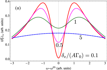
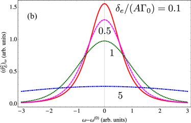
Figure 4: Faraday rotation (a) and ellipticity (b) fluctuation spectra calculated for four different ratios $\delta/(A\Gamma_{0})=0.1$, $0.5$, $1$ and $5$. The origin of frequencies is taken at the precession frequency $\omega^{(0)}=A\omega_{\rm pr}+C$ where the Faraday rotation fluctuations vanish, see text for details.

To model the crossover between these two limits we take a combined distribution of electron spin precession and optical frequencies in the form

$$p(\Omega,\omega_{0})=\frac{1}{\sqrt{\pi}\delta_{e}}\exp{\left(-\frac{(\Omega-A\omega_{0}-C)^{2}}{\delta_{e}^{2}}\right)}p_{0}(\omega_{0}),$$

where the function $p(\omega_{0})$ describes the distribution of optical resonance frequencies and is, hereafter, taken to be flat within the frequency range of interest. The Faraday rotation and ellipticity fluctuation spectra are shown in Fig. 4, panels (a) and (b), respectively.

One can clearly see from Fig. 4 that, with an increase of the spread of electron spin precession frequencies controlled by the parameter $\delta_{e}/(A\Gamma_{0})$, the Faraday rotation spectrum transforms from two-maxima shape with vanishing signal in the middle to the flat spectrum. At the same time, the fluctuations spectrum of ellipticity signal $(\vartheta_{\mathcal{E}}^{2})_{\omega}$ simply widens with an increase of $\delta_{e}/(A\Gamma_{0})$.

V Conclusions

To conclude, we have developed a microscopic theory of electron or hole spin fluctuations in semiconductor quantum dot ensembles. The spin noise spectra are calculated with allowance for the hyperfine or dipole-dipole interaction of the charge carrier spin with lattice nuclei, the Zeeman effect of external magnetic field and inhomogeneous broadening of the electron $g$-factor. The spin noise features related with the spin relaxation and spin decoherence caused by nuclei are identified.

The fluctuation spectra of spin-Faraday and ellipticity effects have been analyzed as well. It is demonstrated that their shape may be strongly affected by the correlation between the optical transition frequency and the electron spin precession frequency.

Appendix A Spin fluctuations in the framework of the fluctuation-dissipation theorem

In the framework of the linear response theoryLandauStat the electron spin fluctuations can be related with the generalized spin susceptibility $\mu_{\alpha\beta}$ describing the linear response of electron spin to the generalized forces $f_{\alpha}$:

$$\delta s_{\alpha,\omega}=\sum_{\beta}\mu_{\alpha\beta}(\omega)f_{\beta,\omega}\>.$$ (26)

In this second description of spin fluctuations equivalent to the description provided by Eqs. (2), (3) and (8), the force ${\bm{f}}(t)$ acts as a perturbation to the spin Hamiltonian LandauStat

$$\hat{V}=-\sum_{\alpha}\hat{s}_{\alpha}f_{\alpha}\>,$$ (27)

where $\hat{s}_{\alpha}$ are the electron spin operators, and can be related to the components of electron spin precession frequency in a random magnetic field as ${\bm{\Omega}}_{\sim}=-{\bm{f}}/\hbar$.

In the presence of the static magnetic field characterized by the spin precession frequency $\bm{\Omega}$, see Eq. (6), the magnetic susceptibility ${\bm{\mu}}(\omega)$ can be found from the kinetic equation for the electron spin $\bm{s}=\bar{\bm{s}}+\delta\bm{s}$, where ${\bar{\bm{s}}\equiv}\bar{\bm{s}}({\bm{\Omega}})$ is the equilibrium spin orientation in the static field with the Larmor frequency ${\bm{\Omega}}$ and $\delta\bm{s}$ is the non-equilibrium spin polarization induced by the weak fluctuating force ${\bm{f}}$ ($|\bm{f}|\ll\hbar|\bm{\Omega}|$):

$$\frac{\partial\bm{s}}{\partial t}+\left[\bm{s}\times\left({\bm{\Omega}}+{\bm{\Omega}}_{\sim}\right)\right]+Q\{\bm{s}\}=0,$$ (28)

where the collision integral of the formslicht

$$Q\{\bm{s}\}=\frac{\bm{s}-\bm{\bar{}}{\bm{s}}\left(\bm{\Omega}+{\bm{\Omega}}_{\sim}\right)}{\tau_{s}}$$ (29)

takes into account the spin relaxation to its equilibrium value for the total field with the Larmor frequency ${\bm{\Omega}}+{\bm{\Omega}}_{\sim}$. Assuming that the Zeeman splitting induced by the external field $\hbar\bm{\Omega}$ is much smaller than the temperature of the system expressed in the units of energy, $k_{B}T$, one has

$$\bar{\bm{s}}({\bm{\Omega}})=-\frac{\hbar{\bm{\Omega}}}{4k_{B}T}\>,\>\bar{\bm{s}}({\bm{\Omega}}+{\bm{\Omega}}_{\sim})=-\frac{\hbar{\bm{\Omega}}-\bm{f}}{4k_{B}T}\>,$$ (30)

where $k_{B}$ is the Boltzmann constant. Hence, the fluctuation $\delta\bm{s}$ satisfies the following linearized equation:

$$-\mathrm{i}\omega\delta\bm{s}+\delta\bm{s}\times\bm{\Omega}+\frac{\delta\bm{s}}{\tau_{s}}=\frac{1}{4k_{B}T}\left(\frac{\bm{f}}{\tau_{s}}-\bm{\Omega}\times\bm{f}\right)\>.$$ (31)

It can be solved by using Eqs. (5) and (9) yielding the spin susceptibility in the form

$$\mu_{\alpha\beta}=\frac{1}{4k_{B}T\tau_{s}}\left[\chi_{\alpha\beta}(\omega)-\sum_{\mu\nu}\chi_{\alpha\mu}(\omega)\delta_{\mu\nu\beta}\Omega_{\nu}\right]\>.$$ (32)

One can readily check that the spin noise spectral functions of Eq. (8), in agreement with the general theory,LandauStat are expressed via the susceptibility $\mu_{\alpha\beta}(\omega)$ as [cf. Ref. kos2010, ]

$$(\delta s_{\alpha}\delta s_{\beta})_{\omega}=\frac{\mathrm{i}k_{B}T}{\omega}\left[\mu_{\beta\alpha}^{*}(\omega)-\mu_{\alpha\beta}(\omega)\right]\>.$$ (33)

This equivalence can be proved by applying the following identity relating bilinear and linear components of the tensor ${\bm{\chi}}$:

$$\sum_{\gamma}\chi_{\alpha\gamma}(\omega)\chi_{\beta\gamma}^{*}(\omega)=\frac{\mathrm{i}}{2\omega}~{}\left\{\chi_{\beta\alpha}^{*}(\omega)-\chi_{\alpha\beta}(\omega)\right.$$ (34)

$$+\sum_{\mu\nu}~{}\left.[\chi_{\alpha\mu}(\omega)\delta_{\mu\nu\beta}-\chi_{\beta\mu}^{*}(\omega)\delta_{\mu\nu\alpha}]\Omega_{\nu}\right\}\>.$$

References

- (1) G. M. Müller, M. Oestreich, M. Römer, and J. Hübner, Physica E 43, 569 (2010).
- (2) S. A. Crooker, D. G. Rickel, A. V. Balatsky, and D. L. Smith, Nature 431, 49 (2004).
- (3) M. Oestreich, M. Römer, R. J. Haug, and D. Hägele, Phys. Rev. Lett. 95, 216603 (2005).
- (4) G. M. Müller, M. Römer, D. Schuh, W. Wegscheider, J. Hübner, and M. Oestreich, Phys. Rev. Lett. 101, 206601 (2008).
- (5) S. A. Crooker, L. Cheng, and D. L. Smith, Phys. Rev. B 79, 035208 (2009).
- (6) S. A. Crooker, J. Brandt, C. Sandfort, A. Greilich, D. R. Yakovlev, D. Reuter, A. D. Wieck, and M. Bayer, Phys. Rev. Lett. 104, 036601 (2010).
- (7) R. Dahbashi, J. Hübner, F. Berski, J. Wiegand, X. Marie, K. Pierz, H. W. Schumacher, and M. Oestreich, Appl. Phys. Lett. 100, 031906 (2012).
- (8) Yan Li, N. Sinitsyn, D. L. Smith, D. Reuter, A. D. Wieck, D. R. Yakovlev, M. Bayer, S. A. Crooker, Phys. Rev. Lett. 108, 186603 (2012).
- (9) E. Aleksandrov and V. Zapasskii, Sov. Phys. JETP 54, 64 (1981) [Zh. Exp. Teor. Fiz. 81, 132 (1981)].
- (10) M. M. Glazov and E. Ya. Sherman, Phys. Rev. Lett. 107, 156602 (2011).
- (11) A. Greilich, D. R. Yakovlev, A. Shabaev, A. L. Efros, I. A. Yugova, R. Oulton, V. Stavarache, D. Reuter, A. Wieck, and M. Bayer, Science 313, 341 (2006).
- (12) A. Greilich, A. Shabaev, D. R. Yakovlev, A. L. Efros, I. A. Yugova, D. Reuter, A. D. Wieck, and M. Bayer, Science 317, 1896 (2007).
- (13) D. Yakovlev and M. Bayer, in Spin physics in semiconductors, Ed. M. Dyakonov, Chap. 6 (Springer, 2008).
- (14) M. M. Glazov, Phys. Solid State 54, 1 (2012) [Fiz. Tverd. Tela 54, 3 (2012)].
- (15) A. V. Khaetskii and Y. V. Nazarov, Phys. Rev. B 64, 125316 (2001).
- (16) L. M. Woods, T. L. Reinecke, and Y. Lyanda-Geller, Phys. Rev. B 66, 161318 (2002).
- (17) V. Kalevich, K. Kavokin, and I. Merkulov, in Spin physics in semiconductors, Ed. by M. Dyakonov, Chap. 11 (Springer, 2008).
- (18) I. A. Merkulov, A. L. Efros, and M. Rosen, Phys. Rev. B 65, 205309 (2002).
- (19) A. V. Khaetskii, D. Loss, and L. Glazman, Phys. Rev. Lett. 88, 186802 (2002).
- (20) M. M. Glazov, I. A. Yugova, and A. L. Efros, Phys. Rev. B 85, 041303 (2012).
- (21) S. Gantsevich, V. Gurevich, and R. Katilius, Riv. Nuovo Cimento 2, 1 (1979).
- (22) L. D. Landau and E. M. Lifshitz, Statistical Physics, Part 1 (Course of Theoretical Physics, Vol. 5), Chap. XII (Butterworth-Heinemann, Oxford, 2000).
- (23) M. Lax, Rev. Mod. Phys. 38, 541 (1966).
- (24) L. P. Pitaevskii and E. M. Lifshitz, Physical Kinetics, Butterworth-Heinemann (Course of Theoretical Physics, Vol. 10), Chap. I (Butterworth-Heinemann, Oxford, 1999).
- (25) I. A. Merkulov, G. Alvarez, D. R. Yakovlev, and T. C. Schulthess, Phys. Rev. B 81, 115107 (2010).
- (26) E. L. Ivchenko, Sov. Phys. Solid State 7, 998 (1974) [Fiz. Tverd. Tela 7, 1489 (1974)].
- (27) Provided that the electron spin relaxation time is much longer than the typical timescale of the nuclear field variation the coupling between electron and nuclear spin may result in slow, , electron spin decay (at ) and, correspondingly, feature in the spin noise spectrum (at , see Refs. coupled, for details. Experimentally, divergent low-frequency spin fluctuations were observed by Yan Li et al in Ref. crooker2012, in the presence of magnetic field.
- (28) R. de Sousa and S. Das Sarma, Phys. Rev. B 67, 033301 (2003); K. A. Al-Hassanieh, V. V. Dobrovitski, E. Dagotto, and B. N. Harmon, Phys. Rev. Lett. 97, 037204 (2006); R.-B. Liu, W. Yao, L. Sham, New Journal of Physics 9, 226 (2007); E. Barnes, L. Cywinski, and S. Das Sarma, Phys. Rev. B 84, 155315 (2011).
- (29) Wenxian Zhang, V. V. Dobrovitski, K. A. Al-Hassanieh, E. Dagotto, and B. N. Harmon, Phys. Rev. B 74, 205313 (2006).
- (30) K. Schulten and P. G. Wolynes, J. Chem. Phys. 68, 3292 (1978).
- (31) E. Gryncharova and V. Perel’, Sov. Phys. Semicond. 11, 997 (1977) [Fiz. Tekhn. Polupr. 11, 1697 (1977)].
- (32) J. Fischer, W. A. Coish, D. V. Bulaev, and D. Loss, Phys. Rev. B 78, 155329 (2008).
- (33) C. Testelin, F. Bernardot, B. Eble, and M. Chamarro, Phys. Rev. B 79, 195440 (2009).
- (34) B. Eble, C. Testelin, P. Desfonds, F. Bernardot, A. Balocchi, T. Amand, A. Miard, A. Lemaître, X. Marie, and M. Chamarro, Phys. Rev. Lett. 102, 146601 (2009).
- (35) M. Braun and J. König, Phys.Rev. B 75 085310 (2007).
- (36) M. M. Glazov and E. L. Ivchenko, Semiconductors 42, 951 (2008) [Fiz. Tekhn. Polupr. 42, 966 (2008)].
- (37) I. A. Yugova, M. M. Glazov, E. L. Ivchenko, and A. L. Efros, Phys. Rev. B 80, 104436 (2009).
- (38) E. L. Ivchenko, Optical Spectroscopy of Semiconductor Nanostructures (Alpha Science, Harrow, UK 2005).
- (39) M. M. Glazov, I. A. Yugova, S. Spatzek, A. Schwan, S. Varwig, D. R. Yakovlev, D. Reuter, A. D. Wieck, and M. Bayer, Phys. Rev. B 82, 155325 (2010).
- (40) Š. Kos, A. V. Balatsky, P. B. Littlewood, and D. L. Smith, Phys. Rev. B 81, 064407 (2010).
- (41) See, e.g., C.P. Slichter, Principles of Magnetic Resonance, Chap. II, V (Springer-Verlag, Berlin, 1980).