Measurements, quantum discord and parity in spin 1 systems

Abstract

We consider the evaluation of the quantum discord and other related measures of quantum correlations in a system formed by a spin $1$ and a complementary spin system. A characterization of general projective measurements in such system in terms of spin averages is thereby introduced, which allows to easily visualize their deviation from standard spin measurements. It is shown that the measurement optimizing these measures corresponds in general to a non-spin measurement. The important case of states that commute with the total $S_{z}$ spin parity is discussed in detail, and the general stationary measurements for such states (parity preserving measurements) are identified. Numerical and analytical results for the quantum discord, the geometric discord and the one way information deficit in the relevant case of a mixture of two aligned spin $1$ states are also presented.

I Introduction

There is presently a great interest in the investigation of quantum correlations and “quantumness” in mixed states of composite quantum systems. While in the case of pure states such correlations can be identified with entanglement, the situation in mixed states is more complex, as separable (i.e., non-entangled) mixed states, defined as convex mixtures of product states RW.89 , can still exhibit signatures of quantum correlations, as the different products may not commute. The interest has been further enhanced by the existence of mixed state based quantum algorithms, such as that of Knill and Laflamme (KL) KL.98 , able to achieve an exponential speed-up over the classical algorithms with no entanglement DFC.05 . In contrast, entanglement is essential for achieving exponential speed-up in pure state based quantum computation JL.03 .

Consequently, alternative measures of quantum correlations for mixed states, such as the quantum discord OZ.01 ; HV.01 ; Zu.03 , have recently received much attention. Though coinciding with entanglement in pure states, discord differs essentially from the latter in mixed states, being non-zero in most separable states and vanishing just for “classically correlated” states, i.e., states which are diagonal in a standard or conditional product basis. The existence of a finite discord in the KL algorithm DSC.08 further increased the interest on this measure. Other measures with similar properties were also recently introduced Lu.08 ; Mo.10 ; DVB.10 ; HH.05 ; RCC.10 ; SKB.11 ; Mo.11 ; GA.12 , including in particular the geometric discord DVB.10 , which allows an easier evaluation. Various fundamental properties Mo.10 ; DVB.10 ; HH.05 ; RCC.10 ; SKB.11 ; Mo.11 ; FF.10 ; FC.11 and operational interpretations SKB.11 ; Mo.11 ; DG.09 ; MD.11 ; CC.11 ; PG.11 ; RRA.11 ; GC.12 ; DL.12 ; TG.12 of these measures were recently unveiled. For instance, from the results of KW.04 it follows that in a pure tripartite system $|\Psi_{ABC}\rangle$, the quantum discord between $C$ and $A$ (as obtained due to a measurement in $C$) is the entanglement of formation Be.96 between $A$ and $B$ plus the conditional entropy $S(A|B)$ CC.11 ; MD.11 ; FC.11 . This entails that such discord provides the entanglement consumption in the extended quantum state merging scheme from $A$ to $B$ CC.11 ; MD.11 . Besides, states with non-zero discord can be used, even if separable, to generate entanglement in the protocols of SKB.11 or PG.11 , with the quantum discord and the one-way information deficit HH.05 ; SKB.11 (a closely related quantity) providing the minimum partial and total distillable entanglement between the measurement apparatus and the system after a von Neumann measurement on the latter SKB.11 . Operational interpretations of the geometric discord were also recently provided DL.12 ; TG.12 . See ref. Mo.11 for a recent review.

A common feature of discord type measures is that they involve a difficult minimization over a general local measurement on one of the system constituents. Consequently, most evaluations were so far restricted to two qubits (two spins $1/2$) or a qubit plus a complementary system, where the most general projective measurement in the local qubit reduces to a standard spin measurement and is hence easy to parameterize OZ.01 ; DVB.10 ; DSC.08 ; AR.10 ; CRC.10 ; GA.11 ; RCC.11 . Closed evaluations in gaussian systems with gaussian type measurements were also achieved GP.10 ; AD.10 . Nonetheless, even for two qubits, general analytic expressions are available just for the geometric discord DVB.10 and some related measures RCC.11 . Here we will examine the evaluation of the quantum discord (and related measures) between a spin $1$ and a complementary spin system. This requires first a convenient characterization of measurements in a spin $1$ system (a qutrit), since they are no longer restricted to standard spin measurements as in the spin $s=1/2$ case, even when considering just standard projective measurements. We provide in sec. II a simple description of such measurements in terms of spin averages, and show that spin measurements are not optimum in general for spin $s\geq 1$, even if the state is described in terms of basic spin observables.

We then analytically identify, in sec. III, the stationary projective measurements for states exhibiting $S_{z}$ parity symmetry, an ubiquitous symmetry present for instance in any non-degenerate eigenstate of spin arrays with $XYZ$ couplings of arbitrary range in a transverse field RCM.09 (for a pair of qubits such symmetry leads to the well-known $X$ states AR.10 ). This allows a considerable simplification of the problem of discord evaluation in parity conserving systems. As application, we present analytical results for the quantum discord, the geometric discord and the one-way information deficit in the important case of a mixture of two aligned spin 1 states. Such mixture represents the reduced state of any spin pair in the ground state of $XYZ$ spin $1$ chains in the immediate vicinity of the transverse factorizing field GAI.08 ; RCM.09 , so that present results represent the universal limit of these quantities at such point. We also explicitly determine the projective measurements minimizing these quantities for this state and show that they exhibit important differences. Conclusions are finally given in IV.

II Measurements in spin systems

II.1 General case

We first consider a spin $s$ system, where we will denote with $\bm{S}=(S_{x},S_{y},S_{z})={\cal S}/\hbar$ the dimensionless angular momentum and $|m\rangle$ the eigenstates of $S_{z}$ (standard basis). Spin measurements are measurements in a basis of eigenstates $|m_{\bm{k}}\rangle=e^{-i\bm{\theta}_{\bm{k}}\cdot\bm{S}}|m\rangle$ of the spin component $\bm{k}\cdot\bm{S}$ along the direction of a unit vector $\bm{k}$, and are then specified by just two real parameters which determine its orientation. For $s\geq 1$ these measurements are, however, only a particular case of complete projective measurement (von Neumann measurement), i.e., those defined by a complete set of rank $1$ orthogonal projectors. The latter are determined by a general unitary transformation of the $S_{z}$ eigenstates,

$$|m_{U}\rangle=U|m\rangle\,,$$ (1)

and depend therefore on $d(d-1)$ real parameters, with $d=2s+1$ ($U=e^{iH}$, with $H$ hermitian, depends on $d^{2}$ real parameters, but just $d^{2}-d$ are sufficient to determine the set of projectors $\{\Pi_{m}^{U}=|m_{U}\rangle\langle m_{U}|\}$ defining the measurement, as the phase of each $|m_{U}\rangle$ is irrelevant). The states (1) are the eigenstates of the operator $S^{U}_{z}=US_{z}U^{\dagger}$, which in general is no longer a linear combination of the original $S_{\mu}$ ($\mu=x,y,z$). Such measurements can, nonetheless, be regarded as measurements of a generalized spin $S^{U}_{z}$ (the algebra $[S^{U}_{\mu},S^{U}_{\nu}]=i\epsilon_{\mu\nu\sigma}S^{U}_{\sigma}$ still holds), and can be implemented as measurements in the standard $S_{z}$ basis preceded by a single qudit gate $U^{\dagger}$.

A first glimpse into the nature of these measurements can be attained through the set of vectors

$$\langle\bm{S}\rangle_{m_{U}}=\langle m_{U}|\bm{S}|m_{U}\rangle\,,$$ (2)

which, in contrast with the case of a spin measurement ($\langle\bm{S}\rangle_{m_{\bm{k}}}=m\bm{k}$), i) may have any length between 0 and $s$ and ii) are not necessarily collinear. Nonetheless, since $\bm{S}$ is traceless, they always sum to zero:

$$\sum_{m}\langle\bm{S}\rangle_{m_{U}}=\bm{0}\,.$$ (3)

While not fully identifying the measurement, the set of averages (2) allow a rapid visualization of its deviation from a standard spin measurement: if $\langle\bm{S}\rangle_{m_{U}}=m\bm{k}$ for $m=-s,\ldots,s$, it is clearly a spin measurement along $\bm{k}$ due to the orthogonality of the basis.

II.2 Spin 1 systems

In the case of a spin $1$ system ($d=3$), Eq. (3) entails that the three vectors (2) are coplanar. Moreover, the operators $S_{z}^{U}$ are at most quadratic functions of the $S_{\mu}$, as any operator in such system can be written as a linear combination of the three $S_{\mu}$ and the six operators $(S_{\mu}S_{\nu}+S_{\nu}S_{\mu})/2$. For example, a non-spin measurement in such system is provided by the states $|m_{\alpha}\rangle=e^{-i\alpha(S_{x}S_{y}+S_{y}S_{x})}|m\rangle$, i.e.,

$$|\pm 1_{\alpha}\rangle=\cos\alpha\,|\pm 1\rangle\pm\sin\alpha\,|\mp 1\rangle,\;|0_{\alpha}\rangle=|0\rangle\,,$$ (4)

which satisfy $S_{z}^{\alpha}|m_{\alpha}\rangle=m|m_{\alpha}\rangle$ with

$$S_{z}^{\alpha}=S_{z}\cos 2\alpha+(S_{x}^{2}-S_{y}^{2})\sin 2\alpha\,.$$

They lead to

$$\langle\bm{S}\rangle_{\pm 1_{\alpha}}=(0,0,\pm\cos\,2\alpha),\;\;\langle\bm{S}\rangle_{0_{\alpha}}=\bm{0}\,,$$

and hence to the second plot in Fig. 1: The vectors $\langle\bm{S}\rangle_{m_{\alpha}}$ are still collinear but $|\langle\bm{S}\rangle_{\pm 1_{\alpha}}|\leq 1$. Moreover, for $\alpha=\pi/4$, $\langle\bm{S}\rangle_{m_{\alpha}}=\bm{0}$ $\forall$ $m$, showing that the average spin may vanish in all elements of the basis: In this case $|\pm 1_{\alpha}\rangle=(|\pm 1\rangle\pm|\mp 1\rangle)/\sqrt{2}$ become the zero eigenstates of $S_{y}$ and $S_{x}$ respectively, which form together with $|0\rangle$ an orthonormal basis.

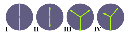
Figure 1: (Color online) Representation of measurements in a spin 1 system through the spin expectation values in the basis states. I: Spin measurement along $z$. II: Collinear measurement, determined by the definite parity states (4) or (5) ($\beta=0$ in (7)). III: $Y$-type measurement, determined by the basis (8)–(10) ($\beta=\pi/4$ in (7)). IV: General measurement, determined by basis (7)–(8).

The most general basis (disregarding global phases and permutations) leading to collinear averages along $z$ for $s=1$ can be obtained by rotating the states (4) around the $z$ axis, which leads to states

$$|m^{\phi}_{\alpha}\rangle=e^{-i\phi S_{z}}|m_{\alpha}\rangle\,.$$ (5)

These are the most general states with definite $S_{z}$ parity:

$$P_{z}|m_{\alpha}^{\phi}\rangle=(-1)^{m+1}|m_{\alpha}^{\phi}\rangle\,,\;\;P_{z}\equiv e^{i\pi(S_{z}+1)}\,.$$ (6)

We now show that the six parameters specifying a general projective measurement in a spin $1$ system can be decomposed into three angles $(\alpha,\beta,\gamma)$ which determine the “intrinsic” plot of vectors $\langle\bm{S}\rangle_{m_{U}}$ (and hence the type of measurement), plus three angles $(\psi,\theta,\phi)$ which determine the orientation of this plot and of the ensuing states. Assuming first $\langle\bm{S}\rangle_{m_{U}}\neq\bm{0}$ for some $m$, we choose the “intrinsic” $z$ axis in the direction of this vector. A state $a|1\rangle+b|0\rangle+c|-1\rangle$ giving rise to $\langle\bm{S}\rangle=(0,0,\langle S_{z}\rangle)$ should satisfy $b\bar{a}+\bar{b}c=0$, which implies $b=0$ if $\langle S_{z}\rangle\neq 0$ ($|a|\neq|c|$). Discarding total phases, the most general orthonormal basis containing such state is then

$$\!\!\!\!\!|{{}^{1_{\bm{r}}}_{0_{\bm{r}}}}\rangle={{}^{\cos\beta}_{\sin\beta}}(e^{-i\phi_{0}}\cos\alpha|1\rangle+e^{i\phi_{0}}\sin\alpha|-1\rangle)\mp{{}^{\sin\beta}_{\cos\beta}}e^{-i\gamma}|0\rangle\,,$$ (7)

$$\!\!\!\!\!|-1_{\bm{r}}\rangle=-e^{-i\phi_{0}}\sin\alpha|1\rangle+e^{i\phi_{0}}\cos\alpha|-1\rangle\,.$$ (8)

where $\bm{r}\equiv(\alpha,\beta,\gamma)$. These states lead in general to non-collinear spin averages of different lengths (plot IV in Fig. 1). Choosing $\phi_{0}$ such that the diagram lies in the intrinsic $x,z$ plane ($\langle S_{y}\rangle_{m_{\bm{r}}}=0$ $\forall$ $m$), we obtain $\tan\phi_{0}=\tan\gamma\tan(\pi/4-\alpha)$ and

$$\langle\bm{S}\rangle_{{}^{1_{\bm{r}}}_{0_{\bm{r}}}} = (\mp\sin 2\beta{\textstyle\sqrt{(1+\cos 2\gamma\sin 2\alpha)/2}},0,{{}^{\cos^{2}\beta}_{\sin^{2}\beta}}\cos 2\alpha)\,,$$

$$\langle\bm{S}\rangle_{-1_{\bm{r}}} = (0,0,-\cos 2\alpha)\,.$$ (9)

Hence, $(\alpha,\beta,\gamma)$ determine respectively $\langle\bm{S}\rangle_{-1_{\bm{r}}}$ and the components of $\langle\bm{S}\rangle_{{0}_{\bm{r}}}$ parallel and orthogonal to $\langle\bm{S}\rangle_{-1_{\bm{r}}}$. Eqs. (9) also show that the angle between vectors $\langle\bm{S}\rangle_{m_{\bm{r}}}$ always exceeds $\pi/2$: $\!\langle\bm{S}\rangle_{m_{\bm{r}}}\cdot\langle\bm{S}\rangle_{m^{\prime}_{\bm{r}}}\leq 0$ if $m\neq m^{\prime}$, vanishing just if one average is zero. The states (7)–(8) can be written as $|m_{\bm{r}}\rangle=e^{i(\gamma(S_{z}^{2}-1)-\phi_{0}S_{z})}e^{-i\alpha(S_{x}S_{y}+S_{y}S_{x})}e^{i\frac{\beta}{\sqrt{2}}(S_{y}+S_{y}S_{z}+S_{z}S_{y})}|m\rangle$.

The most general orthonormal basis is then obtained by applying a general rotation $e^{-i\psi S_{z}}e^{-i\theta S_{y}}e^{-i\phi S_{z}}$ to this basis. This also includes the case $\langle\bm{S}\rangle_{m_{U}}=\bm{0}$ $\forall$ $m$, since such basis are always formed by the zero eigenstates of the components of $\bm{S}$ along three orthogonal directions: For a state $a|1\rangle+b|0\rangle+c|-1\rangle$, the condition $\langle\bm{S}\rangle=\bm{0}$ implies $b\bar{a}+\bar{b}c=0$ and $|a|=|c|$. It is then the eigenstate with zero eigenvalue of $\bm{k}\cdot\bm{S}$, with (assuming, with no loss of generality, $b$ real and $c=-\bar{a}$) $\bm{k}=(-\sqrt{2}{\rm Re}(a),\sqrt{2}{\rm Im}(a),b)$. Orthogonality of the basis states then implies that of the associated vectors $\bm{k}$ (as $\bm{k}\bm{k}^{\prime}=a\bar{a}^{\prime}+bb^{\prime}+\bar{a}a^{\prime}$). Hence, these basis can be obtained, for instance, through a suitable rotation of the intrinsic case $\alpha=\pi/4,\beta=\gamma=0$, where (7)–(8) reduce to the zero eigenstates of $S_{y}$, $S_{z}$ and $S_{x}$.

We may then set $\alpha,\beta\in[0,\pi/4]$ and $\gamma\in(-\pi/2,\pi/2]$ in (7)–(8), as other values can be mapped to these ranges after suitable rotations (disregarding total phases). Notice that if $\gamma\in(0,\pi/2)$ and $\beta\neq 0$, the values $\pm\gamma$ lead to inequivalent and conjugate basis (as $\phi_{0}(-\gamma)=-\phi_{0}(\gamma)$), but the same set of spin averages. The definite parity states (4) are recovered for $\beta=\gamma=0$.

Another relevant case is $\beta=\pi/4$ in (7), where

$$|{{}^{1_{\bm{r}}}_{0_{\bm{r}}}}\rangle={\textstyle\frac{1}{\sqrt{2}}}(e^{-i\phi_{0}}\cos\alpha|1\rangle+e^{i\phi_{0}}\sin\alpha|-1\rangle\mp e^{i\gamma}|0\rangle)\,,$$ (10)

satisfy $P_{z}|^{1_{\bm{r}}}_{0_{\bm{r}}}\rangle=|^{0_{\bm{r}}}_{1_{\bm{r}}}\rangle$, with $P_{z}|-1_{\bm{r}}\rangle=|-1_{\bm{r}}\rangle$, such that parity also leaves this basis (i.e., the set of states) invariant. This also implies $\langle 1_{\bm{r}}|S_{z}|1_{\bm{r}}\rangle=\langle 0_{\bm{r}}|S_{z}|0_{\bm{r}}\rangle$, entailing a symmetric $Y$-type spin diagram (plot III in Fig. 1). For $\alpha=\pi/4$, the $Y$ reduces to an horizontal line and the states (8)–(10) become, for $\gamma=\phi_{0}=0$, eigenstates of $S_{x}$ (as $\langle\bm{S}\rangle_{{}^{0_{\bm{r}}}_{1_{\bm{r}}}}=(\pm 1,0,0)$). The fully symmetric case $\beta=\pi/4$, $\gamma=0$, $\sin 2\alpha=1/3$, where $|\langle\bm{S}\rangle_{m_{\bm{r}}}|^{2}=8/9$ $\forall$ $m$, leads to the maximum total squared spin length: $L_{S}^{2}=\sum_{m}|\langle\bm{S}\rangle_{m_{U}}|^{2}=8/3$, larger than the value $L_{S}^{2}=2$ obtained for a spin measurement.

III Evaluation of Quantum discord and related measures

III.1 General Case

Let us now consider the evaluation of the quantum discord between $n-1$ arbitrary spins $S^{i}$ (system $A$) and a spin $s$ (system $B$), as obtained due to a local complete projective measurement $M_{B}=\{\Pi_{m}^{U}\}$ on system $B$. If initially in a state $\rho_{AB}$, the state of the total system after an unread measurement $M_{B}$ becomes

$$\rho^{\prime}_{AB}=\sum_{m}(I_{A}\otimes\Pi_{m}^{U})\rho_{AB}(I_{A}\otimes\Pi_{m}^{U})\,.$$ (11)

For a local measurement of this type, the quantum discord OZ.01 ; HV.01 can be expressed in terms of (11) as

$$D^{B}(\rho_{AB})=\mathop{\rm Min}_{M_{B}}[S(\rho^{\prime}_{AB})-S(\rho^{\prime}_{B})]-[S(\rho_{AB})-S(\rho_{B})]\,,$$ (12)

where $S(\rho)=-{\rm Tr}\,\rho\log\rho$ is the von Neumann entropy and $\rho_{B}={\rm Tr}_{A}\,\rho_{AB}$ the reduced state of $B$. It can then be considered as the minimum increase of the conditional entropy $S(A|B)=S(A,B)-S(B)$ due to such measurements, and is a non-negative quantity OZ.01 ; HV.01 . For a pure state ($\rho_{AB}^{2}=\rho_{AB}$) it becomes the entanglement entropy $S(\rho_{B})=S(\rho_{A})$, as in this case $S(\rho_{AB})=0$ and $S(\rho^{\prime}_{AB})=S(\rho^{\prime}_{A})$ $\forall$ $M_{B}$ of this form. However, for a mixed state $D^{B}(\rho_{AB})$ vanishes just for classically correlated states with respect to $B$, i.e., states of the form (11) (a particular case of separable state), which are diagonal in a conditional product basis $\{|\nu_{m}\rangle\otimes|m_{U}\rangle\}$ and remain hence unchanged under a particular von Neumann measurement in $B$. Eq. (12) actually provides an upper bound to the quantum discord obtained with general POVM measurements, although results for two-qubits indicate that the difference is very small Mo.11 .

We will also consider here the minimum generalized information loss due an unread local measurement of the previous type RCC.10 ; RCC.11 ,

$$I^{B}_{f}(\rho_{AB})=\mathop{\rm Min}_{M_{B}}S_{f}(\rho^{\prime}_{AB})-S_{f}(\rho_{AB})\,,$$ (13)

where $S_{f}(\rho)={\rm Tr}\,f(\rho)$ denotes a general entropic form, with $f$ a smooth strictly concave function satisfying $f(0)=f(1)=0$ CR.02 . Like $D^{B}$, it can be shown RCC.10 that $I_{f}^{B}(\rho_{AB})\geq 0$ for any such $f$ and $\rho_{AB}$, with $I_{f}^{B}(\rho_{AB})$ becoming the generalized entanglement entropy $S_{f}(\rho_{B})=S_{f}(\rho_{A})$ for a pure state, while for a general mixed state it vanishes just for states of the general form (11), i.e. states diagonal in a conditional product basis. Other properties, including the evaluation of $I_{f}^{B}$ for any $f$ in some specific states (mixture of a pure state with a maximally mixed state, Bell-diagonal states, etc.), were discussed in RCC.10 ; RCC.11 .

Eq. (13) contains as particular cases two important measures: If $f(\rho)=-\rho\log\rho$, $S_{f}(\rho)$ is the von Neumann entropy and Eq. (13) becomes RCC.10 the one way information deficit from $B$ to $A$ HH.05 ; SKB.11 . This quantity is closely related to the quantum discord (12), coinciding with it when the minimizing measurement is the same for both quantities and such that $\rho^{\prime}_{B}=\rho_{B}$ (this occurs for instance when $\rho_{B}$ is maximally mixed, as in Bell diagonal states). It also reduces to the standard entanglement entropy $S(\rho_{A})=S(\rho_{B})$ for pure states. The one-way information deficit has been interpreted as the amount of information that cannot be localized through a classical communication channel from $B$ to $A$ HH.05 ; SKB.11 , and as previously stated, an operational interpretation as the minimum distillable entanglement between the system and the measurement apparatus, was recently provided SKB.11 .

On the other hand, if $f(\rho)=f_{2}(\rho)\equiv\rho(1-\rho)$, $S_{f}(\rho)$ becomes the so called linear entropy $S_{2}(\rho)=1-{\rm Tr}\,\rho^{2}$ and Eq. (13) becomes

$$I_{2}^{B}(\rho_{AB})=\mathop{\rm Min}_{M_{B}}{\rm Tr}\,(\rho_{AB}^{2}-{\rho^{\prime}}_{\!AB}^{2})\,.$$

This quantity is identical RCC.10 with the geometric measure of discord DVB.10 , the latter defined as the minimum squared Hilbert-Schmidt distance from $\rho_{AB}$ to a classically correlated state: $I_{2}^{B}={\rm Min}_{\rho^{\prime}_{AB}}||\rho_{AB}-\rho^{\prime}_{AB}||^{2}$, where $||O||^{2}={\rm Tr}\,O^{\dagger}O$ and $\rho^{\prime}_{AB}$ is a state diagonal in a conditional product basis with respect to $B$. In comparison with the previous measures, the geometric discord offers the advantage of an easier evaluation (yet vanishing for the same type of states), as the calculation of ${\rm Tr}\,\rho^{2}$ does not require the explicit knowledge of the eigenvalues of $\rho$. An analytic expression for general two qubit states was in fact provided in DVB.10 , while its extension to $2\otimes d$ systems was given in GA.12 . An operational interpretation related with the fidelity and performance of remote state preparation BB.01 (a variant of the teleportation protocol) has also been recently provided DL.12 ; TG.12 . Besides, the geometric discord for a $2\otimes d$ system can be measured or estimated with direct non-tomographic methods GA.12 ; JZ.12 ; PM.12 , which provide an experimentally accessible scheme. For pure states $\rho_{AB}$, the geometric discord becomes proportional to the square of the concurrence Ca.03 $C_{AB}=\sqrt{2(1-{\rm Tr}\rho_{B}^{2})}$.

The general stationary condition for Eq. (13) (a necessary condition for the minimizing measurement) reads RCC.11

$$\Delta_{f}^{B}\equiv{\rm Tr}_{A}[f^{\prime}(\rho^{\prime}_{AB}),\rho_{AB}]=0\,,$$ (14)

where $f^{\prime}$ denotes the derivative of $f$. In the case of the quantum discord (12), an additional term $-[f^{\prime}(\rho^{\prime}_{B}),\rho_{B}]$ should be added to (14) to account for the local terms in (12), leading to the modified equation RCC.11

$$\Delta_{D}^{B}\equiv{\rm Tr}_{A}[f^{\prime}(\rho^{\prime}_{AB}),\rho_{AB}]-[f^{\prime}(\rho^{\prime}_{B}),\rho_{B}]=0\,,$$ (15)

where $f(\rho)=-\rho\log\rho$. Since $\Delta_{f}^{B}$ and $\Delta_{D}^{B}$ are antihermitian local operators with zero diagonal elements in the measured basis RCC.11 , they lead to $d(d-1)/2$ complex equations, which determine suitable values of the $d(d-1)$ real parameters defining the measurement in a $d$ dimensional system $B$. They can be solved, for instance, with the gradient method. It is then clear that standard spin measurements, defined by just two real parameters, will not satisfy in general Eq. (14) or (15) for $s>1/2$, and hence cannot be minimum in general. In the spin $1$ case, Eqs. (14) and (15) lead to 6 real equations which determine suitable values of $(\alpha,\beta,\gamma)$ and the three rotation angles.

III.2 States with $S_{z}$ parity symmetry and parity preserving measurements

Let us now examine the important case where $\rho_{AB}$ commutes with the total $S_{z}$ parity,

$$[\rho_{AB},P_{z}^{AB}]=0\,,\;\;P_{z}^{AB}=P_{z}^{A}\otimes P_{z}^{B}\,,$$ (16)

where $P_{z}^{A}=\otimes_{i=1}^{n-1}e^{i\pi(S_{z}^{i}-S^{i})}$. This is an ubiquitous symmetry. For instance, general $XYZ$ type couplings of arbitrary range between spins in a transverse field, not necessarily uniform, lead to a Hamiltonian

$$H=\sum_{i}b_{i}S^{i}_{z}-\sum_{i,j}\sum_{\mu=x,y,z}J^{\mu}_{ij}S^{i}_{\mu}S^{j}_{\mu}\,,$$ (17)

which clearly satisfies $[H,P^{AB}_{z}]=0$, irrespective of the geometry and dimension of the array. The same holds even if terms $\propto S_{x}^{i}S_{y}^{j}$ are also present. Hence, any non-degenerate eigenstate of $H$, as well as the thermal state $\rho_{AB}\propto\exp[-\beta H]$, will fulfill Eq. (16). Moreover, if Eq. (16) holds, parity is also preserved at the local level, i.e. $[\rho_{B},P_{z}^{B}]=0$, as the partial trace involves just diagonal elements in the complementary system $A$. The reduced state of any subgroup of spins will then also commute with the corresponding local $S_{z}$ parity.

We also add that any system described by a Hamiltonian containing just quadratic terms $\propto$ $P_{i}P_{j}$, $Q_{i}Q_{j}$ and $Q_{i}P_{j}$ in standard coordinates and momenta $Q_{i}=\frac{b_{i}+b^{\dagger}_{i}}{\sqrt{2}}$, $P_{i}=\frac{b_{i}-b_{i}^{\dagger}}{\sqrt{2}i}$, with $b_{i},b^{\dagger}_{i}$ boson operators ($[b_{i},b_{j}^{\dagger}]=\delta_{ij}$, $[b_{i},b_{j}]=0$), does commute with the boson number parity $P_{N}=e^{i\pi N}$, where $N=\sum_{i}b^{\dagger}_{i}b_{i}$. Hence, when restricted to a finite $N$ subspace, (i.e., $b^{\dagger}_{i}b_{i}\leq N_{\rm max}$), such system is equivalent to a spin like system whose Hamiltonian commutes with the corresponding $S_{z}$ parity, defining $S^{i}_{z}=b^{\dagger}_{i}b_{i}-N_{\rm max}/2$.

For an arbitrary $\rho_{AB}$ satisfying Eq. (16), parity will be preserved by the measurement $M_{B}$, i.e.,

$$[\rho^{\prime}_{AB},P_{z}^{AB}]=0\,,$$ (18)

when $P_{z}^{B}\Pi_{m}^{U}P_{z}^{B}=\Pi_{m}^{U}$ $\forall$ $m$ and also when $P_{z}^{B}\Pi_{m}^{U}P_{z}^{B}=\Pi_{m^{\prime}}^{U}$, where $\Pi_{m^{\prime}}^{U}$ is another element of the set of local projectors, as in both cases the set will remain invariant: $\{P_{z}^{B}\Pi_{m}^{U}P_{z}^{B}\}=\{\Pi_{m}^{U}\}$. The last case corresponds to $P_{z}^{B}|m_{U}\rangle\propto|m^{\prime}_{U}\rangle$, and since $(P_{z}^{B})^{2}=I_{B}$, such basis can contain just pairs permuted by $P_{z}^{B}$ and isolated eigenstates of $P_{z}^{B}$. For a spin $1$ system, parity will then be preserved for type II as well as type III measurements, i.e., those based on the states (4)–(5) or (8)–(10).

If Eqs. (16)–(18) hold, the commutator in (14) will also commute with $P_{z}^{AB}$, implying

$$[\Delta_{f}^{B},P_{z}^{B}]=0\,,\;\;\;[\Delta_{D}^{B},P_{z}^{B}]=0\,.$$ (19)

This ensures the existence of parity preserving measurements satisfying Eq. (14) or (15), as the number of independent elements which have to vanish is reduced by (19), matching exactly the reduced number of free parameters defining such measurements (essentially $\approx d(d-1)/2$). For instance, in the spin $1$ case and for type II measurements, Eq. (19) implies $(\Delta_{f}^{B})_{m,0}=0$ in the measurement basis and Eq. (14) reduces to a single complex equation ($(\Delta_{f}^{B})_{-1,1}=0$) determining $\alpha,\phi$. For type III measurements, Eq. (19) implies $(\Delta_{f}^{B})_{0,1}$ imaginary and $(\Delta_{f}^{B})_{-1,0}=(\Delta_{f}^{B})_{-1,1}$ in the measured basis, and Eq. (14) leads to one real and one complex equation, which determine $\alpha,\gamma,\phi$. As there is a maximum and a minimum of $I_{f}^{B}$ within these measurements, solutions are ensured. Moreover, if $\Delta_{f}^{B}$ is real in the standard basis, as occurs for instance when $\rho_{AB}$ and all $\Pi_{m}^{U}$ are real in such basis ($\phi=\gamma=0$), Eq. (19) reduces to a single real equation in both measurements:

$$(\Delta_{f}^{B})_{-1,1}=0\,,$$ (20)

which determines the optimum $\alpha$. These arguments also apply for $\Delta_{D}^{B}$, leading to $(\Delta_{D}^{B})_{-1,1}=0$ in the real case.

Parity preserving measurements are then strong candidates for providing the actual minimum of $D^{B}$ or $I_{f}^{B}$, although “parity breaking” solutions of (14) may also exist. The latter are degenerate, as the sets $\{\Pi_{m}^{U}\}$ and $\{P_{z}^{B}\Pi_{m}^{U}P_{z}^{B}\}$ will lead to the same values of $D^{B}$ and $I_{f}^{B}$ when (16) holds. Note also that parity preserving spin measurements are just those along $z$ or an axis perpendicular to $z$ (where $P_{z}|m_{\bm{k}}\rangle\propto|-m_{\bm{k}}\rangle$) and do not have enough parameters for satisfying Eq. (14) if $s\geq 1$. In the real case, just those along $x$, $y$ or $z$ will lead in general to a real $\rho^{\prime}_{AB}$ and no continuous free parameter is left.

III.3 Application

As illustration, we consider a bipartite state formed by the mixture of two aligned spin $1$ states,

$$\rho_{AB}={\textstyle\frac{1}{2}}(|\theta\theta\rangle\langle\theta\theta|+|-\theta-\theta\rangle\langle-\theta-\theta|)\,,$$ (21)

where $|\theta\rangle\equiv e^{-i\theta S_{y}}|1\rangle=|1_{\bm{k}}\rangle$ is the state with maximum spin along $\bm{k}=(\sin\theta,0,\cos\theta)$ (a coherent state). As $P_{z}|\theta\rangle=|-\theta\rangle$, Eq. (21) fulfills Eq. (16). This state arises, for instance, as the reduced state of any spin pair in the fixed parity states

$$|\Psi_{\pm}\rangle=\frac{|\theta\ldots\theta\rangle\pm|-\theta\ldots-\theta\rangle}{\sqrt{2(1\pm\langle-\theta|\theta\rangle^{n})}}\,,$$ (22)

if small overlap terms $\propto\langle-\theta|\theta\rangle^{n-2}$ are neglected ($\langle-\theta|\theta\rangle=\cos^{2s}\theta$) CRC.10 . Such states are the exact ground states of an $XYZ$ spin chain described by (17) in the immediate vicinity of the transverse factorizing field RCM.09 , existing in the case of fixed anisotropy $\chi=\frac{J^{y}_{ij}-J^{z}_{ij}}{J^{x}_{ij}-J^{z}_{ij}}=\cos^{2}\theta$ $\forall$ $i,j$ for $|J^{y}_{ij}|\leq J^{x}_{ij}$, irrespective of the geometry or coupling range.

The state (21) is separable (a convex mixture of product states RW.89 ) $\forall$ $\theta$, but classically correlated just for $\theta=0$ or $\pi/2$ (where $\langle-\theta|\theta\rangle=0$). Accordingly, $D^{B}(\rho_{AB})$ and $I_{f}^{B}(\rho_{AB})$ will be non zero just for $\theta\in(0,\pi/2)$. As the state is symmetric, we have $D^{B}=D^{A}\equiv D$ and $I_{f}^{B}=I_{f}^{A}\equiv I_{f}$. As before, we will consider just von Neumann type local projective measurements $M_{B}$.

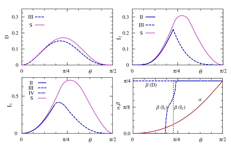
Figure 2: (Color online) The quantum discord $D$ (top left), the geometric discord $I_{2}$ (top right) and the one way information deficit $I_{1}$ (bottom left) of the mixture of aligned states (21) as a function of $\theta$ for spin $s=1$. The dotted lines depict the result obtained with a spin measurement, the other curves the actual minimum, obtained with the indicated measurement (see Fig. 1). The bottom right panel depicts the angles characterizing the minimizing measurement. $D$ is minimized by a parity preserving type III measurement $\forall$ $\theta$ whereas $I_{2}$ changes from type II to III at $\theta=\theta_{c}$, and $I_{1}$ changes from II to III through a small crossover region where a parity breaking type IV measurement is preferred. The angle $\alpha$ is the same for all quantities (Eq. (23)). Normalization is such that $D=I_{2}=I_{1}=1$ for a Bell state.

Results for the quantum discord $D$, the geometric discord $I_{2}$ and the one-way information deficit (denoted here as $I_{1}$) are shown in Fig. 2. It is first confirmed that minimization over spin measurements provides just an upper bound to the actual value of these quantities, being nonetheless a good approximation for small $\theta$. The qualitative behavior of these three quantities is similar (they are all maximum for $\theta$ slightly below $\pi/4$), but important differences in the minimizing measurement do arise. While $D$ is minimized by a real ($\phi=\gamma=0$) type III measurement $\forall$ $\theta\in(0,\pi/2)$, leading to a smooth curve, $I_{2}$ prefers a real type II (III) measurement for $\theta<\theta_{c}$ ($>\theta_{c}$), exhibiting a II–III “transition” and hence a cusp maximum at $\theta=\theta_{c}$. The same holds for $I_{1}$ except that the transition between the collinear and $Y$-type measurements is smoothed through an intermediate region ($0.19\pi\lesssim\theta\lesssim 0.24\pi)$ where a parity breaking measurement ($\gamma=0$, $0<\beta<\pi/4$ in (7)) is preferred. These features resemble then the $s=1/2$ case CRC.10 ; RCC.11 , where $D$ preferred a spin measurement along $x$ $\forall$ $\theta$ CRC.10 whereas $I_{2}$ exhibited a sharp $z\rightarrow x$ transition, with $I_{1}$ selecting a parity breaking axis in a small intermediate interval RCC.11 . Hence, for $s=1$, parity preserving type II and III measurements play the role of the $z$ and $x$ measurements respectively of the $s=1/2$ case.

Remarkably, the minimizing value of $\alpha$, obtained from Eq. (20), is the same for $D$, $I_{2}$ and $I_{1}$ in all previous cases $\forall\theta$ (i.e., for both type II and III measurements):

$$\tan\alpha=\tan^{2}\theta/2\,.$$ (23)

At this value the largest eigenvalue of $\rho^{\prime}_{AB}$ is maximum and $\rho^{\prime}_{AB}$ attains certain majorizing properties. The evaluation of these measures becomes then analytic. For instance, the quantum and geometric discords read

$$D = 2h_{\frac{1}{2}}(p_{\theta})-1-h_{1}[2q_{\theta}(1-q_{\theta})]+h_{1}(q_{\theta})\,,$$ (24)

$$I_{2} = \left\{{}^{\frac{1}{8}\sin^{4}\theta(3+\cos 2\theta)^{2}\,,\;\;\theta<\theta_{c}}_{\frac{1}{16}\cos^{4}\theta(11+4\cos 2\theta+\cos 4\theta)\,,\;\;\theta>\theta_{c}}\right.\,,\;\;\cos\theta_{c}={\textstyle\frac{1}{\sqrt[4]{3}}}\,,$$ (25)

where $h_{\nu}(x)=-x\log_{2}x-(\nu-x)\log_{2}(\nu-x)$, $p_{\theta}=\frac{1}{4}-\frac{1}{16}(\frac{115}{8}-\cos 2\theta+\frac{3}{2}\cos 4\theta+\cos 6\theta+\frac{1}{8}\cos 8\theta)^{1/2}$ and $q_{\theta}=\frac{1}{2}\sin^{2}\theta$. Remarkably, $\theta_{c}\approx 0.23\pi$ in $I_{2}$ is determined by the overlap condition $\langle-\theta|\theta\rangle^{2}=1/3$, as in the $s=1/2$ case RCC.11 , with $I_{2}=2/9$ at $\theta=\theta_{c}$ (the same value as for $s=1/2$). For $\theta\rightarrow 0$, $D\approx\theta^{2}$ while $I_{2}\approx 2\theta^{4}$ (similar to the $s=1/2$ case CRC.10 ; RCC.11 ), whereas for $\theta\rightarrow\pi/2$, $D\approx[\frac{1}{2}-\frac{\log_{2}e}{4}-\log_{2}(\frac{\pi}{2}-\theta)](\frac{\pi}{2}-\theta)^{4}$ while $I_{2}\approx\frac{1}{2}(\frac{\pi}{2}-\theta)^{4}$. In this limit $D$ and $I_{2}$ are then proportional to the overlap $\langle-\theta|\theta\rangle^{2}=\cos^{4s}\theta$. We also mention that for small $\theta$, the difference between the approximate value of $D$ obtained with spin measurements and the actual $D$ is very small ($O(-\theta^{6}\log_{2}\theta)$), while in the case of $I_{2}$ and $I_{1}$, such difference is $O(\theta^{4})$ (i.e., of leading order in $I_{2}$).

IV Conclusions

We have first provided a simple characterization of orthogonal projective measurements in spin $1$ systems, which can be extended to arbitrary spin and allows a rapid visualization of the (projective) measurements optimizing discord-type measures of quantum correlations. Standard spin measurements are not optimum in general for minimizing such measures for spin $s\geq 1$. Instead, we have shown that for the relevant case of states with parity symmetry, parity preserving measurements provide stationary solutions for all these measures. We have identified such measurements for spin $1$, where they are described by just two or three parameters (or one in the real case) allowing to considerably simplify the variational problem associated with discord. Results for the mixture (21), which represents the state of any spin pair in an XYZ chain in the immediate vicinity of the factorizing field, confirm the optimality of such measurements in most cases. They also confirm the distinct behavior of the minimizing measurement in the quantum discord as compared to that in the geometric discord (or other measures of type (13) like the information deficit). The latter are more sensible to changes in the nature of the state and hence more suitable for identifying transitions between different regimes.

The authors acknowledge support of CIC (RR) and CONICET (JMM,NC) of Argentina.

References

- (1) R.F. Werner, Phys. Rev. A 40, 4277 (1989).
- (2) E. Knill, R. Laflamme, Phys. Rev. Lett. 81, 5672 (1998).
- (3) A. Datta, S.T. Flammia and C.M. Caves, Phys. Rev. A 72, 042316 (2005).
- (4) R. Josza and N. Linden, Proc. R. Soc. A459, 2011 (2003); G. Vidal, Phys. Rev. Lett. 91, 147902 (2003).
- (5) H. Ollivier, W.H. Zurek, Phys. Rev. Lett. 88 017901 (2001).
- (6) L. Henderson and V. Vedral, J. Phys. A 34, 6899 (2001); V. Vedral, Phys. Rev. Lett. 90, 050401 (2003).
- (7) W. H. Zurek, Phys. Rev. A 67, 012320 (2003).
- (8) A. Datta, A. Shaji, and C.M. Caves, Phys. Rev. Lett. 100, 050502 (2008).
- (9) S. Luo, Phys. Rev. A 77, 042303 (2008).
- (10) K. Modi et al, Phys. Rev. Lett. 104, 080501 (2010).
- (11) B. Dakić, V. Vedral, and Č. Brukner, Phys. Rev. Lett. 105, 190502 (2010).
- (12) M. Horodecki et al Phys. Rev. A 71, 062307 (2005); J. Oppenheim et al Phys. Rev. Lett. 89, 180402 (2002).
- (13) R. Rossignoli, N. Canosa, L. Ciliberti, Phys. Rev. A 82, 052342 (2010).
- (14) A. Streltsov, H. Kampermann, and D. Bruß, Phys. Rev. Lett. 106, 160401 (2011).
- (15) K. Modi et al, arXiv: 1112.6238 (2011).
- (16) D. Girolami, G. Adesso, Phys. Rev. Lett. 108 150403 (2012).
- (17) A. Ferraro et al, Phys. Rev. A 81, 052318 (2010).
- (18) F.F. Fanchini et al, Phys. Rev. A 84, 012313 (2011).
- (19) A. Datta, S. Gharibian, Phys. Rev. A 79, 042325 (2009).
- (20) V. Madhok, A. Datta, Phys. Rev. A 83, 032323 (2011).
- (21) D. Cavalcanti et al, Phys. Rev. A 83, 032324 (2011).
- (22) M. Piani et al, Phys. Rev. Lett. 106, 220403 (2011).
- (23) L. Roa, J.C. Retamal, M. Alid-Vaccarezza, Phys. Rev. Lett. 107, 080401 (2011).
- (24) M. Gu et al, arXiv:1203.0011 (2012).
- (25) B. Dakić et al, arXiv:1203.1629 (2012).
- (26) T. Tufarelli et al, arXiv:1205.0251 (2012).
- (27) M. Koashi, A. Winter, Phys. Rev. A 69, 022309 (2004).
- (28) C.H. Bennett et al, Phys. Rev. A 54, 3824 (1996).
- (29) M. Ali, A.R.P. Rau, G. Alber, Phys. Rev. A 81, 042105 (2010); ibid. 82, 069902(E) (2010).
- (30) L.Ciliberti, R. Rossignoli, N. Canosa, Phys. Rev. A 82, 042316 (2010).
- (31) D. Girolami, G. Adesso, Phys. Rev. A 83 052108 (2011).
- (32) R. Rossignoli, N. Canosa, L. Ciliberti, Phys. Rev. A 84, 052329 (2011).
- (33) P. Giorda, M.G.A. Paris, Phys. Rev. Lett. 105, 020503 (2010).
- (34) G. Adesso, A. Datta, Phys. Rev. Lett. 105, 030501 (2010); L. Mišta et al, Phys. Rev. A 83, 042325 (2011).
- (35) R. Rossignoli, N. Canosa, J.M. Matera, Phys. Rev. A 77, 052322 (2008); ibid 80, 062325 (2009).
- (36) S.M. Giampaolo, G. Adesso, F. Illuminati, Phys. Rev. B 79, 224434 (2009); Phys. Rev. Lett. 100, 197201 (2008).
- (37) N. Canosa, R. Rossignoli, Phys. Rev. Lett. 88 170401 (2002).
- (38) C.H. Bennett et al, Phys. Rev. Lett. 87, 077902 (2001).
- (39) J-S.Jin et al, J. Phys. A 45, 115308 (2012).
- (40) G. Passante, O. Moussa, R. Laflamme, Phys. Rev. A 85, 032325 (2012).
- (41) P. Rungta and C.M. Caves, Phys. Rev. A 67, 012307 (2003); P. Rungta et al, Phys. Rev. A 64, 042315 (2001).