Model independent constraints on leptoquarks from $b\to s\ell^{+}\ell^{-}$ processes

Abstract

We list all scalar and vector leptoquark states that contribute to the $b\to s\ell^{+}\ell^{-}$ effective Hamiltonian. There are altogether three scalar and four vector leptoquarks that are relevant. For contribution of each state we infer the correlations between effective operators and find that only two baryon number-violating vector leptoquarks give rise to scalar and pseudoscalar four-fermion operators, whereas the scalar states can contribute to those operators only when two states with same charge are present. We bound the resulting Wilson coefficients by imposing experimental constraints coming from branching fractions of $B\to K\ell^{+}\ell^{-}$, $B_{s}\to\mu^{+}\mu^{-}$, and $B\to X_{s}\mu^{+}\mu^{-}$ decays.

I Introduction

The $b\to s\ell^{+}\ell^{-}$ induced processes have been recognized as very important probes of the Standard Model and new physics. Rare decay $B_{s}\to\mu^{+}\mu^{-}$ has been subject to intensive experimental efforts Abazov et al. (2010); *Aaltonen:2011fi; *Chatrchyan:2011kr; *PhysRevLett.108.231801 at Fermilab and LHC and currently the upper bound on the branching ratio has been set slightly above the Standard Model (SM) prediction. Increasing statistics in this decay mode at the LHC will soon allow to probe the SM prediction directly Buras (2003). Exclusive $B\to K^{(*)}\ell^{+}\ell^{-}$ and inclusive $B\to X_{s}\ell^{+}\ell^{-}$ decays with $\ell=e,\mu$ offer many different observables to be confronted against the theoretical predictions. Their studies at the $B$-meson factories Iwasaki et al. (2005); Aubert et al. (2004); Sun et al. (2012) and at the LHCb experiment Aaij et al. (2012b) indicate that all observables are, within relatively large error bars, compatible with the predictions of the SM Alok et al. (2011); *Drobnak:2011aa; *Bobeth:2011nj; *Beaujean:2012uj; *Mahmoudi:2012un; *Altmannshofer:2012ir.

The leptonic branching fraction, $\mathrm{Br}(B_{s}\to\mu^{+}\mu^{-})$, is very sensitive to physics beyond the SM where scalar or pseudoscalar four-fermion operators are present, namely, such contributions are helicity-enhanced with respect to the SM amplitude. Complementary information on those operators can be extracted from the spectrum of semileptonic $B\to K\ell^{+}\ell^{-}$ decay. Indeed, the leptonic and semileptonic decay widths depend on orthogonal combinations of (axial-)vector current and (pseudo)scalar four-fermion operators Becirevic et al. (2012a). Size of the vector and axial-vector current operators can also be assessed by studying the transverse asymmetries in $B\to K^{*}\ell^{+}\ell^{-}$ decay Kruger and Matias (2005); *Becirevic:2011bp.

Scalar and pseudoscalar operators are present in new physics (NP) models where a color- and charge-neutral scalar particle produces the lepton pair, as is the case in supersymmetric extensions of the SM. Another possibility to generate $b\to s\ell^{+}\ell^{-}$ at short distances is an exchange of a color triplet particles that couple to a lepton-quark pair. Such leptoquark states have spin either 0 and 1 and are present in Grand Unified Theories Georgi and Glashow (1974); *PhysRevLett.64.619; *Dorsner:2005fq, Pati-Salam models Pati and Salam (1974), composite scenarios Schrempp and Schrempp (1985); *Gripaios:2009dq, or technicolor models Kaplan (1991). However, since a leptoquark naturally generates Fierzed operators of the form $(\bar{s}\Gamma\ell)(\bar{\ell}\Gamma b)$, the scalar operators,

$$(\bar{s}P_{L(R)}b)(\bar{\ell}\ell)\,,\qquad(\bar{s}P_{L(R)}b)(\bar{\ell}\gamma_{5}\ell)\,,$$ (1)

cannot be identified with exchanges of a scalar leptoquarks. In a similar way, a vector leptoquark exchange does not necessarily induce vector current operators.

Leptoquarks have been studied extensively in the literature. For early model independent studies see e.g. Buchmuller et al. (1987); *Leurer:1993em; *Davidson:1993qk; *PhysRevD.56.5709, while for some recent works see Alikhanov (2012); *Saha:2010vw; *Dighe:2010nj; *Carpentier:2010ue; *Bobeth:2011st; *Dorsner:2011ai. In this work we complement the SM with a single leptoquark state and assume all other degrees of freedom lie substantially higher above the electroweak scale. The tree-level contributions to $b\to s\ell^{+}\ell^{-}$ due to a single colored particle exchange present a very constrained framework. A lepton and a down-type quark combine into a color triplet current to which a colored state with electric charge $2/3$ or $4/3$ can couple. The two charge assignments of the leptoquark correspond to fermion numbers $F=0$ and $F=2$ of the bilinear, where $F=3B+L$, and $B$ and $L$ are baryon and lepton numbers (see Fig. 1).

Figure 1: Two possible charges of a leptoquark in $b\to s\ell^{+}\ell^{-}$ diagram.

Our aim here is to consider one by one leptoquarks that potentially contribute to the $b\to s\ell^{+}\ell^{-}$ transitions, determine correlations between effective operators affecting the $b\to s\ell^{+}\ell^{-}$ effective Hamiltonian, and constrain the underlying couplings from experimental data on $B_{s}\to\mu^{+}\mu^{-}$, $B\to K\ell^{+}\ell^{-}$, and $B\to X_{s}\mu^{+}\mu^{-}$ decays.

II Effective Hamiltonian

The effective Hamiltonian of dimension-6 at the mass scale of $b$ quark reads Grinstein et al. (1989); *Misiak:1992bc; *Buras:1994dj

$$\mathcal{H}_{\mathrm{eff}}=- \frac{4G_{F}}{\sqrt{2}}\lambda_{t}\Big{[}\sum_{i=1}^{6}C_{i}(\mu)\mathcal{O}_{i}(\mu)$$ (2)

$$+\sum_{i=7,8,9,10,P,S}\left(C_{i}(\mu)\mathcal{O}_{i}(\mu)+C^{\prime}_{i}(\mu)\mathcal{O}^{\prime}_{i}(\mu)\right)$$

$$+C_{T}\mathcal{O}_{T}+C_{T5}\mathcal{O}_{T5}\Big{]}\,,$$

where $\lambda_{t}=V_{tb}V_{ts}^{*}$. Effective operators that receive contributions from leptoquarks are the two-quark, two-lepton operators,

$$\mathcal{O}_{9} =\frac{e^{2}}{g^{2}}(\bar{s}\gamma_{\mu}P_{L}b)(\bar{\ell}\gamma^{\mu}\ell)\,,$$ (3)

$$\mathcal{O}_{10} =\frac{e^{2}}{g^{2}}(\bar{s}\gamma_{\mu}P_{L}b)(\bar{\ell}\gamma^{\mu}\gamma_{5}\ell)\,,$$

$$\mathcal{O}_{S} =\frac{e^{2}}{16\pi^{2}}(\bar{s}P_{R}b)(\bar{\ell}\ell)\,,$$

$$\mathcal{O}_{P} =\frac{e^{2}}{16\pi^{2}}(\bar{s}P_{R}b)(\bar{\ell}\gamma_{5}\ell)\,.$$

$$\mathcal{O}_{T} =\frac{e^{2}}{16\pi^{2}}(\bar{s}\sigma^{\mu\nu}b)(\bar{\ell}\sigma_{\mu\nu}\ell)\,,$$

$$\mathcal{O}_{T5} =\frac{e^{2}}{16\pi^{2}}(\bar{s}\sigma^{\mu\nu}b)(\bar{\ell}\sigma_{\mu\nu}\gamma_{5}\ell)\,.$$

The chirally flipped operators $\mathcal{O}^{\prime}_{9,10,S,P}$ are obtained from the above ones by $L\leftrightarrow R$ exchange. $e=\sqrt{4\pi\alpha}$ is the unit of electric charge, $g$ is the strong coupling, and $P_{L,R}=(1\mp\gamma_{5})/2$. Four-quark operators $\mathcal{O}_{1\ldots 6}$ and radiative penguin operators $\mathcal{O}_{7,8}$ can be found in ref. Bobeth et al. (2000). Values of the Wilson coefficients are calculated by means of matching the full theory onto the effective theory at the electroweak scale and subsequently solving the renormalization group equations to run them down to scale $\mu_{b}=4.8\mathrm{\leavevmode\nobreak\ GeV}$. Decay amplitudes are conveniently expressed in terms of effective Wilson coefficients at the scale $\mu_{b}$ Buras et al. (1994); *Altmannshofer:2008dz,

$$C_{7}^{\rm eff}(\mu_{b}) =\frac{4\pi}{\alpha_{s}}\,C_{7}-\frac{1}{3}\,C_{3}-\frac{4}{9}\,C_{4}-\frac{20}{3}\,C_{5}\,-\frac{80}{9}\,C_{6}\,,$$

$$C_{9}^{\rm eff}(\mu_{b}) =\frac{4\pi}{\alpha_{s}}\,C_{9}+Y(q^{2})\,,$$

$$C_{10}^{\rm eff}(\mu_{b}) =\frac{4\pi}{\alpha_{s}}\,C_{10}\,,\qquad C_{7,8,9,10}^{\prime,\rm eff}(\mu_{b})=\frac{4\pi}{\alpha_{s}}\,C^{\prime}_{7,8,9,10}\,,$$ (4)

where function $Y(q^{2})$ was defined in Altmannshofer et al. (2009). For the SM contributions we will use the NNLL values $C_{7}^{{\text{eff}},\mathrm{SM}}(\mu_{b})=-0.304$, $C_{9}^{{\text{eff}},\mathrm{SM}}(\mu_{b})=4.211$, and $C_{10}^{{\text{eff}},\mathrm{SM}}(\mu_{b})=-4.103$ Bobeth et al. (2000); *Altmannshofer:2008dz. Numerical values of other parameters entering theoretical predictions can be found in Becirevic et al. (2012a).

The diagrams on Fig. 1 will contribute to the Wilson coefficients of operators (3). We will assume that a leptoquark state lies at a scale $\sim 1\mathrm{\leavevmode\nobreak\ TeV}$, still perfectly allowed by limits set by the direct searches Abramowicz et al. (2012); *Abazov:2006vc; *Khachatryan:2010mq; *ATLAS:2012aq; *Aad:2011ch, where we also perform the tree-level matching. For our purposes we can neglect the anomalous dimensions of coefficients $C_{9}^{(\prime)}$ and $C_{10}^{(\prime)}$ Bobeth et al. (2004), whereas the anomalous dimensions of scalar and pseudoscalar Wilson coefficients run with the same anomalous dimension as $m_{b}(\mu)$ Logan and Nierste (2000). Lepton flavor universality of all beyond the SM contributions will be assumed throughout this work in order to make a straightforward interpretation of experimental constraint from $\mathrm{Br}(B\to K\ell^{+}\ell^{-})$ where a result given in Sun et al. (2012) is a combination of $\ell=e$ and $\ell=\mu$ modes.

In the following sections we will omit the “eff” label when writing down beyond the SM contributions to the effective Wilson coefficients.

III Observables and their Standard Model predictions

The $B_{s}\to\ell^{+}\ell^{-}$ decay branching fraction in a general NP model reads

$$\mathrm{Br}\left(B_{s}\to\ell^{+}\ell^{-}\right)= \tau_{B_{s}}f_{B_{s}}^{2}m_{B_{s}}^{3}\frac{G_{F}^{2}|\lambda_{t}|^{2}\alpha^{2}}{(4\pi)^{3}}\beta_{\ell}(m_{B_{s}}^{2})$$ (5)

$$\times\left[\frac{m_{B_{s}}^{2}}{m_{b}^{2}}\Big{|}C_{S}-C_{S}^{\prime}\Big{|}^{2}\left(1-{4m_{\ell}^{2}\over m_{B_{s}}^{2}}\right)\right.\left.+\ \Big{|}{m_{B_{s}}\over m_{b}}\left(C_{P}-C_{P}^{\prime}\right)+2{m_{\ell}\over m_{B_{s}}}\left(C_{10}-C_{10}^{\prime}\right)\Big{|}^{2}\,\right]\,,$$

where $\beta_{\ell}(q^{2})=\sqrt{1-4m_{\ell}^{2}/q^{2}}$. The above branching fraction is sensitive exclusively to contributions of differences between operators with left- and right-handed quark currents, $C_{10}-C_{10}^{\prime}$, $C_{S}-C_{S}^{\prime}$, and $C_{P}-C_{P}^{\prime}$. The latter two combinations are effectively constrained due to lifted helicity suppression unless the relative phases of Wilson coefficients allow cancellations between $C_{S}\,(C_{P})$ and $C_{S}^{\prime}\,(C_{P}^{\prime})$. In the SM only $C_{10}$ is present in (5) and leads to prediction Becirevic et al. (2012a)

$$\mathrm{Br}(B_{s}\to\mu^{+}\mu^{-})_{\mathrm{SM}}=(3.3\pm 0.3)\times 10^{-9}\,,$$ (6)

whereas the latest $95\,\%$ confidence level bound from the LHCb experiment Aaij et al. (2012a) is

$$\mathrm{Br}(B_{s}\to\mu^{+}\mu^{-})_{\mathrm{exp}}<4.5\times 10^{-9}\,.$$ (7)

The decay branching fraction, $\mathrm{Br}(B\to K\ell^{+}\ell^{-})$, on the other hand, receives contributions from $C_{7}+C_{7}^{\prime}$, $C_{9}+C_{9}^{\prime}$, $C_{10}+C_{10}^{\prime}$, $C_{S}+C_{S}^{\prime}$, and $C_{P}+C_{P}^{\prime}$, while we have neglected contribution of the tensor operators that have small contributions in leptoquark models, as will be shown below. The decay width reads Bobeth et al. (2007)

$$\Gamma(B\to K\ell^{+}\ell^{-})=2\left(A_{\ell}+\frac{1}{3}C_{\ell}\right)\,,$$ (8)

where $A_{\ell}$ corresponds to the $\theta$-independent component of the spectrum, whereas $C_{\ell}$ stems from the component proportional to $\cos^{2}\theta$, where $\theta$ is the angle between $\bar{B}$ and $\ell^{-}$ in the rest frame of the lepton pair. They are expressed as integrals over the dilepton invariant mass between $q_{\mathrm{min}}^{2}=4m_{\ell}^{2}$ and $q^{2}_{\mathrm{max}}=(m_{B}-m_{K})^{2}$,

$$A_{\ell} =\int_{q_{\rm min}^{2}}^{q_{\rm max}^{2}}a_{\ell}(q^{2})dq^{2}\,,\qquad C_{\ell}=\int_{q_{\rm min}^{2}}^{q_{\rm max}^{2}}c_{\ell}(q^{2})dq^{2}\,.$$ (9)

The corresponding spectra are

$$a_{\ell}(q^{2})= \ {\cal C}(q^{2})\Big{[}q^{2}\left(\beta_{\ell}^{2}(q^{2})\lvert F_{S}(q^{2})\rvert^{2}+\lvert F_{P}(q^{2})\rvert^{2}\right)+\frac{\lambda(q^{2})}{4}\left(\lvert F_{A}(q^{2})\rvert^{2}+\lvert F_{V}(q^{2})\rvert^{2}\right)$$

$$\hskip 64.01869pt+4m_{\ell}^{2}m_{B}^{2}\lvert F_{A}(q^{2})\rvert^{2}+2m_{\ell}\left(m_{B}^{2}-m_{K}^{2}+q^{2}\right)\text{Re}\left(F_{P}(q^{2})F_{A}^{\ast}(q^{2})\right)\Big{]}\,,$$

$$c_{\ell}(q^{2})= \ {\cal C}(q^{2})\Big{[}-\frac{\lambda(q^{2})}{4}\beta_{\ell}^{2}(q^{2})\left(\lvert F_{A}(q^{2})\rvert^{2}+\lvert F_{V}(q^{2})\rvert^{2}\right)\Big{]}\,,$$

where

$$F_{V}(q^{2})= \left(C_{9}+C_{9}^{\prime}\right)f_{+}(q^{2})+\frac{2m_{b}}{m_{B}+m_{K}}\left(C_{7}+C_{7}^{\prime}\right)f_{T}(q^{2})\,,$$

$$F_{A}(q^{2})= \left(C_{10}+C_{10}^{\prime}\right)f_{+}(q^{2})\,,$$

$$F_{S}(q^{2})= \frac{m_{B}^{2}-m_{K}^{2}}{2m_{b}}\left(C_{S}+C_{S}^{\prime}\right)f_{0}(q^{2})\,,$$

$$F_{P}(q^{2})= \frac{m_{B}^{2}-m_{K}^{2}}{2m_{b}}\left(C_{P}+C_{P}^{\prime}\right)f_{0}(q^{2})-m_{\ell}\left(C_{10}+C_{10}^{\prime}\right)\left[f_{+}(q^{2})-\frac{m_{B}^{2}-m_{K}^{2}}{q^{2}}\left(f_{0}(q^{2})-f_{+}(q^{2})\right)\right]\,.$$

The auxiliary functions are defined as

$$\mathcal{C}(q^{2}) =\frac{G_{F}^{2}\alpha^{2}\lvert\lambda_{t}\rvert^{2}}{512\pi^{5}m_{B}^{3}}\beta_{\ell}(q^{2})\sqrt{\lambda(q^{2})}\,,$$ (10)

$$\lambda(q^{2}) =q^{4}+m_{B}^{4}+m_{K}^{4}-2\left(m_{B}^{2}m_{K}^{2}+m_{B}^{2}q^{2}+m_{K}^{2}q^{2}\right)\,.$$

Functions $F_{X}$, where $X=V,A,S,P$, corresponding to different Lorentz structures in the effective Hamiltonian, are products of the short distance Wilson coefficients and appropriate hadronic form factors of $B\to K$ transition, defined as follows:

$$\langle K(k)|\bar{s}\gamma_{\mu}b|B(p)\rangle= \left[(p+k)_{\mu}-{m_{B}^{2}-m_{K}^{2}\over q^{2}}q_{\mu}\right]f_{+}(q^{2})$$ (11)

$$+{m_{B}^{2}-m_{K}^{2}\over q^{2}}q_{\mu}f_{0}(q^{2})\,,$$

$$\langle K(k)|\bar{s}\sigma_{\mu\nu}b|B(p)\rangle =i\left(p_{\mu}k_{\nu}-p_{\nu}k_{\mu}\right)\frac{2f_{T}(q^{2})}{m_{B}+m_{K}}\,.$$ (12)

The form factors we use were obtained by simulations of QCD on the lattice Zhou et al. (2011); *Becirevic:2012fy; *BecPrep and using QCD sum rules on the light cone Ball and Zwicky (2005); *Khodjamirian:2006st. Details about their parameterization and numerical values have been discussed recently in Becirevic et al. (2012a), where the following SM prediction has been made,

$$\mathrm{Br}\left(B\to K\ell^{+}\ell^{-}\right)_{\mathrm{SM}}=(7.0\pm 1.8)\times 10^{-7}\,.$$ (13)

Recently, BaBar experiment reported a combined measurement of $B^{0}\,(B^{+})\to K^{0}\,(K^{+})\ell^{+}\ell^{-}$ Sun et al. (2012)

$${\rm Br}\left(B\to K\ell^{+}\ell^{-}\right)_{\rm BaBar}=(4.7\pm 0.6\pm 0.2)\times 10^{-7}\,,$$ (14)

that is compatible with the SM prediction (13), while the LHCb experiment Aaij et al. (2012b) found a significantly smaller result for neutral $B$ decays to a muon final state

$${\rm Br}\left(B^{0}\to K^{0}\mu^{+}\mu^{-}\right)_{\rm LHCb}=(3.1^{+0.7}_{-0.6})\times 10^{-7}\,.$$ (15)

Assuming lepton flavor universality, naïve average of the two constraints gives $\mathrm{Br}(B\to K\ell^{+}\ell^{-})=(3.8\pm 0.6)\times 10^{-7}$, but since the two measurements are only marginally compatible we consider in our analysis a range of allowed values that covers both measurements

$$\mathrm{Br}(B\to K\ell^{+}\ell^{-})_{\mathrm{exp}}=(2.5-5.5)\times 10^{-7}\,.$$ (16)

The inclusive decay $B\to X_{s}\mu^{+}\mu^{-}$ will also play an important role in constraining the vector operators $C_{9,10}^{(\prime)}$. Using the formulas presented in Huber et al. (2008); *lunghi-hiller we get for the SM prediction in the lower range of $q^{2}$

$$\int_{1\ \mathrm{\leavevmode\nobreak\ GeV}^{2}}^{6\ \mathrm{\leavevmode\nobreak\ GeV}^{2}}{d{\rm Br}\left(B\to X_{s}\mu^{+}\mu^{-}\right)\over dq^{2}}dq^{2}\Big{|}_{\rm SM}=1.59(17)\times 10^{-6}\,,$$ (17)

where we have kept explicit dependence on $m_{b,\mathrm{pole}}^{5}$, contained in the normalization factor

$$\mathcal{B}_{0}=\tau_{B}\ {4\ \alpha^{2}\ G_{F}^{2}|\lambda_{t}|^{2}\ m_{b,\mathrm{pole}}^{5}\over 3\ (4\pi)^{5}}=3.41(47)\times 10^{-7}\,,$$ (18)

instead of normalizing it to the branching fraction of semileptonic $B\to X_{c}\ell\nu$ decay. Leptoquark-induced additive contributions to the above prediction will be calculated by employing formulas presented in Fukae et al. (2000) in the approximation $m_{\ell}=m_{s}=0$. The partial branching ratio at low $q^{2}$’s has been measured at the $B$-factories Iwasaki et al. (2005); *babar-incl, resulting in an average Huber et al. (2008),

$$\int_{1\mathrm{\leavevmode\nobreak\ GeV}^{2}}^{6\mathrm{\leavevmode\nobreak\ GeV}^{2}}{d{\rm Br}\left(B\to X_{s}\mu^{+}\mu^{-}\right)\over dq^{2}}dq^{2}\Big{|}_{\rm exp}=1.6(5)\times 10^{-6}\,.$$ (19)

IV Scalars

Scalar leptoquarks typically originate from the scalar representations of the unification group that are required to break either the unification or the SM gauge group. We distinguish $Q=2/3$ and $Q=4/3$ cases below.

IV.1 $Q=2/3$ scalars

Charge $2/3$ scalar leptoquarks can couple to leptons and quarks when their chiralities are different, therefore only $\overline{d_{L}}\ell_{R}$ or $\overline{d_{R}}\ell_{L}$ bilinears are allowed in the interaction. Here and in the following $d$ denotes one of the down-type quarks. The two scalars that can form renormalizable vertices with these bilinears transform as doublets under $SU(2)_{L}$,

$$\Delta^{(7/6)} \equiv(3,2)_{7/6}\,,$$ (20)

$$\Delta^{(1/6)} \equiv(3,2)_{1/6}\,.$$

The SM quantum numbers have been specified as $(SU(3)_{c},SU(2)_{L})_{Y}$ and the hypercharge is defined as $Y=Q-T_{3}$. Both states conserve baryon ($B$) and lepton numbers ($L$). The state $\Delta^{(7/6)}$ will couple to the right-handed (RH) leptons in a gauge invariant term

$$\mathcal{L}^{(7/6)}=g_{R}\,\overline{Q}\Delta^{(7/6)}\ell_{R}+\mathrm{h.c.}\,,$$ (21)

that contains a coupling of the $T_{3}=-1/2$ component of $\Delta^{(7/6)}$ to down-quarks and RH leptons. To keep the notation clean, we have omitted flavor indices on the Yukawa couplings $g_{R}$ and fields. Color indices are always contracted between the leptoquark and the quark field. We integrate out $\Delta^{(7/6)}$ and rotate the Yukawa couplings to the quark mass-basis by a redefinition $D_{L}^{\dagger}g_{R}\to g_{R}$, where $D_{L}$ connects the mass and gauge bases as $d_{L}^{\mathrm{gauge}}=D_{L}d_{L}^{\mathrm{mass}}$. The effective Hamiltonian (2) will receive contributions to operators with vector and axial-vector lepton currents

$$C_{9}=C_{10}=\frac{-\pi}{2\sqrt{2}G_{F}\lambda_{t}\alpha}\frac{(g_{R})_{s\ell}(g_{R})_{b\ell}^{*}}{M_{\Delta^{(7/6)}}^{2}}\,.$$ (22)

On the other hand, the state $\Delta^{(1/6)}$ couples via $T_{3}=1/2$ isospin component to the left-handed (LH) leptons as

$$\mathcal{L}^{(1/6)}=g_{L}\,\overline{d_{R}}\tilde{\Delta}^{(1/6)\dagger}L+\mathrm{h.c.}\,,\qquad\tilde{\Delta}\equiv i\tau_{2}\Delta^{*}\,.$$ (23)

Here $\tilde{\Delta}$, defined with the help of the second Pauli matrix $\tau_{2}$, transforms as $(\bar{3},2)_{-1/6}$. This state leaves imprint on operators with RH quark currents and with vector and axial-vector lepton currents

$$-C_{9}^{\prime}=C_{10}^{\prime}=\frac{-\pi}{2\sqrt{2}G_{F}\lambda_{t}\alpha}\frac{(g_{L})_{s\ell}(g_{L})_{b\ell}^{*}}{M_{\Delta^{(7/6)}}^{2}}\,.$$ (24)

We have rotated the couplings to the mass basis by redefinition $D_{R}^{\dagger}g_{L}\to g_{L}$.

Notice that scalar and pseudoscalar operators are not induced by those two states since each of them couples exclusively either to LH or to RH leptons whereas operators $\mathcal{O}_{S,P}^{(\prime)}$ involve both lepton and quark chiralities. However, if we expand our approach and allow for presence of both states we see that they weakly mix since the quantum numbers of $\Delta^{(7/6)}_{T_{3}=-1/2}$ and $\Delta^{(1/6)}_{T_{3}=+1/2}$ are equal in the broken electroweak (EW) phase Hirsch et al. (1996). The mixing term at the EW scale reads

$$\mathcal{L}_{\mathrm{mix}}^{7/6-1/6} =\xi(H^{\dagger}\Delta^{(7/6)})(H^{\dagger}\tilde{\Delta}^{(1/6)})+\mathrm{h.c.}\,,$$ (25)

where $H$ is the Higgs doublet, and $\xi$ is a dimensionless parameter. The above mixing between the two otherwise $B$ and $L$ conserving leptoquarks violates $L$ by $-2$ and $B$ by $2/3$. Radiative generation of Majorana masses for neutrinos in a similar setting has been considered in Aristizabal Sierra et al. (2008). The EW symmetry breaking generates nondiagonal terms in mass matrix for states $(\Delta^{(7/6)}_{T_{3}=1/2},\Delta^{(1/6)}_{T_{3}=-1/2})$

$$\begin{pmatrix}M_{\Delta^{(7/6)}}^{2}&\frac{\xi^{*}v^{2}}{2}\\ \frac{\xi v^{2}}{2}&M_{\Delta^{(1/6)}}^{2}\end{pmatrix}\,,$$ (26)

where $v=246\,$GeV is the vacuum expectation value of the Higgs field. The heavy and light mass eigenstates, $\Delta_{H}$, $\Delta_{L}$, are mixtures of states $\Delta^{(7/6)}$ and $\Delta^{(1/6)}$ (without $T_{3}$ labels from now on). To illustrate consequences in that setting let us consider a case when $M_{\Delta^{(1/6)}}\ll M_{\Delta^{(7/6)}}$. The mass eigenstates are

$$\begin{pmatrix}\Delta_{H}\\ \Delta_{L}\end{pmatrix}=\begin{pmatrix}1&\frac{\xi v^{2}}{2|\Delta M^{2}|}\\ -\frac{\xi^{*}v^{2}}{2|\Delta M^{2}|}&1\end{pmatrix}\begin{pmatrix}\Delta^{(7/6)}\\ \Delta^{(1/6)}\end{pmatrix}\,,$$ (27)

to leading order in mixing parameter, $|\xi|v^{2}/|\Delta M^{2}|$, where $|\Delta M^{2}|=|M_{\Delta^{(1/6)}}^{2}-M_{\Delta^{(7/6)}}^{2}|$. Consequently, the lighter of the two states will decrease its mass by $|\xi|v^{2}/(8\sqrt{|\Delta M^{2}|})$ while mass of the heavier state will increase by the same amount. In turn we generate, in addition to $C_{9}^{\prime}$ and $C_{10}^{\prime}$ in (24), an entire set of scalar, pseudoscalar, and tensor operators:

$$C_{P} =C_{S}=\frac{-\pi}{4\sqrt{2}G_{F}\lambda_{t}\alpha}\frac{\xi v^{2}\,(g_{R})_{s\ell}(g_{L})^{*}_{b\ell}}{M_{\Delta^{(1/6)}}^{2}M_{\Delta^{(7/6)}}^{2}}\,,$$ (28)

$$-C_{P}^{\prime} =C_{S}^{\prime}=\frac{-\pi}{4\sqrt{2}G_{F}\lambda_{t}\alpha}\frac{\xi^{*}v^{2}\,(g_{L})_{s\ell}(g_{R})^{*}_{b\ell}}{M_{\Delta^{(1/6)}}^{2}M_{\Delta^{(7/6)}}^{2}}\,,$$

$$C_{T} =(C_{S}+C_{S}^{\prime})/4\,,$$

$$C_{T5} =(C_{S}-C_{S}^{\prime})/4\,.$$

Same form of expressions for the Wilson coefficients (28) and mixing matrix apply in the inverse mass hierarchy case, with $\Delta^{(7/6)}$ light and $\Delta^{(1/6)}$ heavy, provided we relabel $(7/6)\leftrightarrow(1/6)$ and $\xi\leftrightarrow\xi^{*}$. In this case also $C_{9}$ and $C_{10}$ of Eq. (22) are present.

IV.2 $Q=4/3$ scalars

This case corresponds to a scalar that couples to “clashing” fermion flows of quark and lepton fields. Their chiralities are equal in this case due to the well known identity $(\psi_{L})^{C}=(\psi^{C})_{R}$, stating that a charge-conjugate of left-handed field transforms as a right-handed field under the Lorentz group. Scalar bilinears that participate in vertices are therefore $\overline{d_{L}^{C}}\ell_{L}$ and $\overline{d_{R}^{C}}\ell_{R}$, with $\psi^{C}\equiv C\bar{\psi}^{T}$ and $C$ is a unitary, antisymmetric charge-conjugation matrix in spinor space. We find a weak triplet and singlet states that couple to those bilinears,

$$\Delta^{(1/3)} \equiv(\bar{3},3)_{1/3}\,,$$ (29)

$$\Delta^{(4/3)} \equiv(\bar{3},1)_{4/3}\,.$$

The isotriplet state couples exclusively to LH, whereas the isosinglet couples to the RH fermions. They both form vertices with two quarks which makes them baryon and lepton number violating, $B-L$ conserving leptoquarks. The isotriplet $\Delta^{(1/3)}$ interaction with two fermionic doublets contains the relevant term involving the $T_{3}=+1$ component

$$\mathcal{L}^{(1/3)} =\frac{g_{L}}{\sqrt{2}}\,\overline{Q^{C}}i\tau_{2}\bm{\tau}\cdot\bm{\Delta}^{(1/3)}L+\mathrm{h.c.}$$ (30)

$$=g_{L}\,\overline{d_{L}^{C}}\ell_{L}\Delta^{(1/3)}_{T_{3}=+1}+\cdots\,.$$

A vector of Pauli matrices $\bm{\tau}$ has been introduced. The presence of LH fields in the above interaction implies that only left-handed quark currents can be generated at low scale. After performing a weak-to-mass basis transition, $D_{L}^{T}g_{L}\to g_{L}$, and integrating out the state, we find

$$C_{9}=-C_{10}=\frac{\pi}{2\sqrt{2}G_{F}\lambda_{t}\alpha}\frac{(g_{L})_{b\ell}(g_{L})^{*}_{s\ell}}{M_{\Delta^{1/3}}^{2}}\,.$$ (31)

For the isosinglet state $\Delta^{(4/3)}$ the interaction term with the RH fermions reads

$$\mathcal{L}^{(4/3)}=g_{R}\,\overline{d_{R}^{C}}\ell_{R}\Delta^{(4/3)}+\mathrm{h.c.}\,.$$ (32)

On the effective Hamiltonian level operators with RH quark currents are generated

$$C_{9}^{\prime}=C_{10}^{\prime}=\frac{\pi}{2\sqrt{2}G_{F}\lambda_{t}\alpha}\frac{(g_{R})_{b\ell}(g_{R})^{*}_{s\ell}}{M_{\Delta^{(4/3)}}^{2}}\,,$$ (33)

where $D_{R}^{T}g_{R}\to g_{R}$ rotation has been performed along with transition to the mass basis of fermions.

The above two scalars have same charge and can therefore mix. We can write down the off-diagonal Higgs-induced isotriplet-isosinglet mixing as  Hirsch et al. (1996)

$$\mathcal{L}_{\mathrm{mix}}^{1/3-4/3}=\frac{\xi}{\sqrt{2}}\left(\tilde{H}^{\dagger}\bm{\tau}\cdot\bm{\Delta}^{(1/3)}H\right)\Delta^{(4/3)*}+\mathrm{h.c.}\,,$$ (34)

and find the same expression (27) for the resulting eigenstates, provided we replace $\Delta^{(7/6)}\to\Delta^{(1/3)}$ and $\Delta^{(1/6)}\to\Delta^{(4/3)}$. In the limit $M_{\Delta^{(4/3)}}\ll M_{\Delta^{(1/3)}}$ the scalar and tensor coefficients are

$$C_{P} =C_{S}=\frac{\pi}{4\sqrt{2}G_{F}\lambda_{t}\alpha}\frac{\xi v^{2}\,(g_{R})_{b\ell}(g_{L})^{*}_{s\ell}}{M_{\Delta^{(4/3)}}^{2}M_{\Delta^{(1/3)}}^{2}}\,,$$ (35)

$$-C_{P}^{\prime} =C_{S}^{\prime}=\frac{\pi}{4\sqrt{2}G_{F}\lambda_{t}\alpha}\frac{\xi^{*}v^{2}\,(g_{L})_{b\ell}(g_{R})^{*}_{s\ell}}{M_{\Delta^{(4/3)}}^{2}M_{\Delta^{(1/3)}}^{2}}\,,$$

$$-C_{T} =(C_{S}^{\prime}+C_{S})/4\,,$$

$$C_{T5} =(C_{S}^{\prime}-C_{S})/4\,.$$

In conclusion, we notice that a single scalar leptoquark contributes to one of the following 4 operators

$$\mathcal{O}_{9}^{(\prime)}\pm\mathcal{O}_{10}^{(\prime)}$$ (36)

of the $b\to s\ell^{+}\ell^{-}$ effective Hamiltonian. This is simply due to absence of a scalar color-triplet state with couplings to both chiralities of fermions, which are necessary to form scalar or tensor operators. They are all chiral leptoquarks Leurer (1994b) with regard to their couplings to down-type quarks and charged leptons. Even in the presence of two scalar leptoquarks that are allowed to mix and thus give rise to scalar, pseudoscalar, and tensor operators we find that Wilson coefficients corresponding to those contributions are additionally suppressed by $v^{2}/M_{\Delta}^{2}$ and are therefore less important at low energies.

V Vectors

Vector leptoquark states, if fundamental particles, are typically the remnants of the underlying gauge bosons of the broken unification group Leurer (1994b). They can also be composite states  Schrempp and Schrempp (1985); *Gripaios:2009dq.

V.1 $Q=2/3$ vectors

Vector currents with $3B+L=0$ always involve fermions with equal chiralities, leading in this case to $\overline{d_{L}}\gamma^{\mu}\ell_{L}$ and $\overline{d_{R}}\gamma^{\mu}\ell_{R}$ as the only two allowed bilinears to which vector particles can couple to. There are two vector leptoquarks that contain an appropriate charge 2/3 component,

$$V^{(3)} \equiv(3,3)_{2/3}\,,$$ (37)

$$V^{(1)} \equiv(3,1)_{2/3}\,.$$

First, the isotriplet state is $B$ and $L$ conserving and interacts with LH fermions as

$$\mathcal{L}^{(3)}=g_{L}\,\overline{Q}\,\bm{\tau}\cdot\bm{V}^{(3)}_{\mu}\gamma^{\mu}L+\mathrm{h.c.}\,,$$ (38)

and will, after being integrated out, contribute to the left-handed quark currents:

$$C_{9}=-C_{10}=\frac{\pi}{\sqrt{2}G_{F}\lambda_{t}\alpha}\frac{(g_{L})_{s\ell}(g_{L})^{*}_{b\ell}}{M^{2}_{V^{(3)}}}\,.$$ (39)

Couplings have been redefined as $D_{L}^{\dagger}g_{L}\to g_{L}$. The isosinglet state, $V^{(1)}$, on the other hand has couplings to both LH and RH fermions, i.e. it is a nonchiral leptoquark,

$$\mathcal{L}^{(1)}=\left(g_{L}\,\overline{Q}\gamma^{\mu}L+g_{R}\,\overline{d_{R}}\gamma^{\mu}\ell_{R}\right)\,V^{(1)}_{\mu}+\mathrm{h.c.}\,.$$ (40)

In addition, $B$ is not conserved as $V^{(1)}$ can decay to two down quarks. Because of both chiralities involved, this state contributes to both RH and LH quark currents, as well as to scalar and pseudoscalar operators,

$$C_{9} =-C_{10}=\frac{\pi}{\sqrt{2}G_{F}\lambda_{t}\alpha}\frac{(g_{L})_{s\ell}(g_{L})^{*}_{b\ell}}{M_{V^{(1)}}^{2}}\,,$$ (41)

$$C_{9}^{\prime} =C_{10}^{\prime}=\frac{\pi}{\sqrt{2}G_{F}\lambda_{t}\alpha}\frac{(g_{R})_{s\ell}(g_{R})^{*}_{b\ell}}{M_{V^{(1)}}^{2}}\,,$$

$$-C_{P} =C_{S}=\frac{\sqrt{2}\pi}{G_{F}\lambda_{t}\alpha}\frac{(g_{L})_{s\ell}(g_{R})^{*}_{b\ell}}{M_{V^{(1)}}^{2}}\,,$$

$$C_{P}^{\prime} =C_{S}^{\prime}=\frac{\sqrt{2}\pi}{G_{F}\lambda_{t}\alpha}\frac{(g_{R})_{s\ell}(g_{L})^{*}_{b\ell}}{M_{V^{(1)}}^{2}}\,.$$

V.2 $Q=4/3$ vectors

Similar as in the case of $Q=2/3$ scalars, vector leptoquarks with charge $4/3$ form vertices with quarks and leptons of different chiralities, i.e. $\overline{d_{R}^{C}}\gamma^{\mu}\ell_{L}$ and $\overline{d_{R}^{C}}\gamma^{\mu}\ell_{R}$. An isodoublet state

$$V^{(2)}\equiv(\bar{3},2)_{5/6}\,,$$ (42)

induces both LH and RH lepton couplings,

$$\mathcal{L}^{(2)} =g_{R}\,\overline{Q^{C}}\,i\tau_{2}V^{(2)}_{\mu}\gamma^{\mu}\ell_{R}+g_{L}\,\overline{d_{R}^{C}}\,\gamma^{\mu}\,\tilde{V}^{(2)\dagger}_{\mu}L+\mathrm{h.c.}$$ (43)

$$=-V_{\mu}^{(2),T_{3}=+1/2}\left[g_{R}\,(\overline{d_{L}^{C}}\gamma^{\mu}\ell_{R})+g_{L}\,(\overline{d_{R}^{C}}\gamma^{\mu}\ell_{L})\right]+\cdots\,.$$

The four possible combinations of these then enter the Wilson coefficients as

$$C_{9} =C_{10}=\frac{-\pi}{\sqrt{2}G_{F}\lambda_{t}\alpha}\frac{(g_{R})_{b\ell}(g_{R})^{*}_{s\ell}}{M_{V^{(2)}}^{2}}\,,$$ (44)

$$-C_{9}^{\prime} =C_{10}^{\prime}=\frac{\pi}{\sqrt{2}G_{F}\lambda_{t}\alpha}\frac{(g_{L})_{b\ell}(g_{L})^{*}_{s\ell}}{M_{V^{(2)}}^{2}}\,,$$

$$C_{P} =C_{S}=\frac{\sqrt{2}\pi}{G_{F}\lambda_{t}\alpha}\frac{(g_{R})_{b\ell}(g_{L})^{*}_{s\ell}}{M_{V^{(2)}}^{2}}\,,$$

$$-C_{P}^{\prime} =C_{S}^{\prime}=\frac{\sqrt{2}\pi}{G_{F}\lambda_{t}\alpha}\frac{(g_{L})_{b\ell}(g_{R})^{*}_{s\ell}}{M_{V^{(2)}}^{2}}\,.$$

Processes that lead to $B$ non-conservation are induced via interaction terms of $V^{(1)}$ with two quarks

$$\mathcal{L}^{(1)}_{qq}=\overline{Q^{C}}\,i\tau_{2}\tilde{V}_{\mu}^{(2)}\gamma^{\mu}u_{R}+\mathrm{h.c.}\,.$$ (45)

VI Constraints on leptoquark-induced effective interactions

In each case studied in the previous sections the obtained set of Wilson coefficients follows relations between vector and axial leptonic currents, namely, we can always express $C_{10}^{(\prime)}$ and $C_{P}^{(\prime)}$ with $C_{9}^{(\prime)}$ and $C_{S}^{(\prime)}$, respectively, as

$$\left(\begin{array}[]{r}C_{10}\\ C_{10}^{\prime}\\ C_{P}\\ C_{P}^{\prime}\end{array}\right)=\pm\left(\begin{array}[]{r}C_{9}\\ -C_{9}^{\prime}\\ C_{S}\\ -C_{S}^{\prime}\end{array}\right)\,.$$ (46)

Positive sign on the right-hand side applies for contributions of the scalars $\Delta^{(7/6)}$, $\Delta^{(1/6)}$ and the vector state $V^{(2)}$, whereas the negative sign is valid for Wilson coefficients generated by the the scalars $\Delta^{(4/3)}$, $\Delta^{(1/3)}$, and vectors $V^{(2)}$ and $V^{(1)}$. The contributions of the seven leptoquark states to the effective Hamiltonian are restated in Table 1 where we have already employed the identity (46) to express all Wilson coefficients in terms of complex $C_{10}$, $C_{10}^{\prime}$, $C_{S}$, and $C_{S}^{\prime}$ that can be chosen independently (they can be found in shaded columns of Tab. 1). Because all the Wilson coefficients are invariant under rescaling of the underlying leptoquark couplings

$$(g_{L,R})_{s\ell} \to\zeta(g_{L,R})_{s\ell}\qquad(\zeta\in\mathbb{C})\,,$$ (47)

$$(g_{L,R})_{b\ell} \to\frac{1}{\zeta^{*}}(g_{L,R})_{b\ell}\,,$$

we can further eliminate one complex degree of freedom, say $C_{10}$, by employing

$$4C_{10}C_{10}^{\prime}=-C_{S}C_{S}^{\prime}\,.$$ (48)

Only the vector states $V^{(1)}$ and $V^{(2)}$ implement the most general framework where the current-current $\mathcal{O}^{(\prime)}_{9,10}$ and scalar/pseudoscalar $\mathcal{O}^{(\prime)}_{S,P}$ operators are present. Remaining states have $C_{S}^{(\prime)}=C_{P}^{(\prime)}=0$ and therefore contribute either to $C_{10}$ or $C_{10}^{\prime}$ (and their $C_{9}^{(\prime)}$ partners, see eq. (46)) as can be seen from (48). In fact, a combination of (pseudo)scalar and tensor operators could also arise due to presence of two scalar states with same electric charge, however, we have demonstrated in the previous section those operators are further suppressed by factor $v^{2}/M_{\Delta}^{2}$ and are therefore omitted from Tab. 1 and from further study. Same table also shows that leptoquarks that conserve baryon number and therefore cannot trigger nucleon decay Nath and Fileviez Perez (2007); *Dorsner:2012nq, are limited to contributions to operators with vector and axial-vector leptonic currents. These states, $\Delta^{(7/6)}$, $\Delta^{(1/6)}$, and $V^{(3)}$, can lie at or below the $1\mathrm{\leavevmode\nobreak\ TeV}$ scale and therefore produce visible effects in $b\to s\ell^{+}\ell^{-}$ processes. Effects of those states and $\Delta^{(4/3)}$ are in the focus of this section. We do not delve into study of $B$-violating vector leptoquarks that require more thorough analysis due to presence of many operators as well as due to their potential effect on nucleon stability.

S	LQ	BNC	$\mathcal{O}_{9}$	$\mathcal{O}_{10}$	$\mathcal{O}_{S}$	$\mathcal{O}_{P}$	$\mathcal{O}_{9}^{\prime}$	$\mathcal{O}_{10}^{\prime}$	$\mathcal{O}_{S}^{\prime}$	$\mathcal{O}_{P}^{\prime}$
$0$	$\Delta^{(7/6)}$	✓	$C_{10}$	$\bm{C_{10}}$
	$\Delta^{(1/6)}$	✓					$-C_{10}^{\prime}$	$\bm{C_{10}^{\prime}}$
	$\Delta^{(4/3)}$						$C_{10}^{\prime}$	$\bm{C_{10}^{\prime}}$
	$\Delta^{(1/3)}$		$-C_{10}$	$\bm{C_{10}}$
$1$	$V^{(3)}$	✓	$-C_{10}$	$\bm{C_{10}}$
	$V^{(1)}$		$-C_{10}$	$\bm{C_{10}}$	$\bm{C_{S}}$	$-C_{S}$	$C_{10}^{\prime}$	$\bm{C_{10}^{\prime}}$	$\bm{C_{S}^{\prime}}$	$C_{S}^{\prime}$
	$V^{(2)}$		$C_{10}$	$\bm{C_{10}}$	$\bm{C_{S}}$	$C_{S}$	$-C_{10}^{\prime}$	$\bm{C_{10}^{\prime}}$	$\bm{C_{S}^{\prime}}$	$-C_{S}^{\prime}$

Table 1: Scalar and vector leptoquark tree-level contributions to $(\bar{s}b)(\bar{\ell}\ell)$ effective Hamiltonian. Third column (BNC) indicates whether baryon number is conserved. Wilson coefficients in the shaded columns ($C_{10}$, $C_{10}^{\prime}$, $C_{S}$, and $C_{S}^{\prime}$) are taken as independent. See text for clarification on number of independent parameters for the last two states.

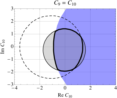
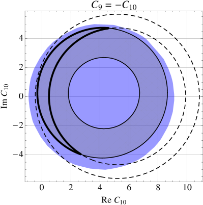
Figure 2: Allowed regions in the complex $C_{10}$ plane in the leptoquark scenario where $C_{9}=C_{10}$ (upper plot) or $C_{9}=-C_{10}$ (lower plot). Blue region corresponds to $\mathrm{Br}(B_{s}\to\mu^{+}\mu^{-})$, whereas the light gray region and dashed lines mark the $\mathrm{Br}(B\to K\mu^{+}\mu^{-})$ and $B\to X_{s}\mu^{+}\mu^{-}$ constraints, respectively. The intersection of all three constraints is thickly outlined. We observe complementarity of the three constraints in the upper and their degeneracy in the lower plot.

VI.1 $C_{9}=\pm C_{10}$

These two scenarios are realized by scalar $\Delta^{(7/6)}$ with the $+$ sign and by vector $V^{(3)}$ with the $-$ sign. They cannot be distinguished by the $C_{9}$-independent constraint $\mathrm{Br}(B_{s}\to\mu^{+}\mu^{-})$, whereas the $\mathrm{Br}(B\to K\ell^{+}\ell^{-})$ and partial branching fraction of $B\to X_{s}\mu^{+}\mu^{-}$ decay depend crucially on the relative sign between $C_{9}$ and $C_{10}$. Beyond the SM contribution to the inclusive decay spectrum can be adapted from formulas in ref. Fukae et al. (2000),

$$\frac{d\mathrm{Br}(B\to X_{s}\mu^{+}\mu^{-})}{d\hat{s}}=2\mathcal{B}_{0}(1-\hat{s})^{2}\Big{[}(1+2\hat{s})\big{\{}C_{10}^{\mathrm{SM}}\mathrm{Re}\left[C_{10}\right]$$

$$\hskip 28.45274pt\pm\mathrm{Re}\left[C_{9}^{\mathrm{SM}}(\hat{s})\,C_{10}^{\ast}\right]+|C_{10}|^{2}\big{\}}\mp 6C_{7}^{\mathrm{SM}}\mathrm{Re}\left[C_{10}\right]\Big{]}\,,$$ (49)

where $\hat{s}=q^{2}/m_{b,\mathrm{pole}}^{2}$ and the choice of sign should follow $C_{9}=\pm C_{10}$. We show in Fig. 2 how the three experimental constraints (7), (16), (19), map onto the $C_{10}$ plane when we confront them with theoretical predictions. Important information in these two cases comes from the measured $B\to K\ell^{+}\ell^{-}$ while the effectiveness of $B\to X_{s}\mu^{+}\mu^{-}$ and the leptonic decay $B_{s}\to\mu^{+}\mu^{-}$ depends on relative sign between $C_{9}$ and $C_{10}$. In the $C_{9}=C_{10}$ case ($\Delta^{(7/6)}$ scalar leptoquark) the $B\to K\ell^{+}\ell^{-}$ decay gives the strongest constraint, however large negative values of $C_{10}$ are effectively excluded also by $B_{s}\to\mu^{+}\mu^{-}$ due to positive interference with the SM. This is a clear demonstration how decreasing experimental bound on $B_{s}\to\mu^{+}\mu^{-}$ is becoming more and more constraining even for vector and axial-vector operators. The opposite relative sign between $C_{9}$ and $C_{10}$ ($V^{(3)}$ vector leptoquark) allows for a finely tuned phase of $C_{10}$ when one can effectively cancel contributions to $\mathrm{Br}(B\to K\ell^{+}\ell^{-})$ and $B\to X_{s}\mu^{+}\mu^{-}$. One can even decrease the two branching fractions and therefore the lower end of the experimental predictions also become relevant in this case.

The overlapping regions of the three constraints give for the size of leptoquark contributions

$$|C_{9,10}|\lesssim\left\{\begin{array}[]{lcl}4&;&C_{9}=C_{10}\\ 6&;&C_{9}=-C_{10}\end{array}\right.\,.$$ (50)

VI.2 $C_{9}^{\prime}=\pm C_{10}^{\prime}$

Scalar leptoquarks that couple to the right-handed fermions belong into this category. States $\Delta^{(4/3)}$ and $\Delta^{(1/6)}$ will induce such contributions with $+$ and $-$ sign, respectively. Shift of the inclusive decay spectrum relatively to the SM prediction can be written in these two cases as

$$\frac{d\mathrm{Br}(B\to X_{s}\mu^{+}\mu^{-})}{d\hat{s}}=2\mathcal{B}_{0}(1-\hat{s})^{2}(1+2\hat{s})|C_{10}^{\prime}|^{2}\,.$$ (51)

We have neglected the interference terms proportional to $m_{s}$ and therefore the inclusive branching fraction is insensitive to the phase of $C_{9}^{\prime}$. One way to distinguish the two scenarios is to measure precisely $B\to K\ell^{+}\ell^{-}$ that exhibits striking sensitivity on the relative sign between $C_{9}^{\prime}$ and $C_{10}^{\prime}$, as shown on Fig. 3. The allowed regions satisfy

$$|C_{9,10}^{(\prime)}|\lesssim 2\,,$$ (52)

for both cases. However, a closer look at Fig. 3 reveals that tension between the $\mathrm{Br}(B_{s}\to\mu^{+}\mu^{-})$ and $\mathrm{Br}(B\to K\ell^{+}\ell^{-})$ in scenario $C_{9}^{\prime}=-C_{10}^{\prime}$ forces the Wilson coefficients to develop CP violating imaginary part. The constraint from $B_{s}\to\mu^{+}\mu^{-}$ is identical in the two cases and excludes a sizeable portion of parameter space only in the case of flipped sign scenario ($C_{9}^{\prime}=-C_{10}^{\prime}$). On the other hand, the inclusive decay is less sensitive to the RH current operators since the interference terms between NP and the SM amplitude are suppressed by $m_{s}$.

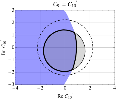
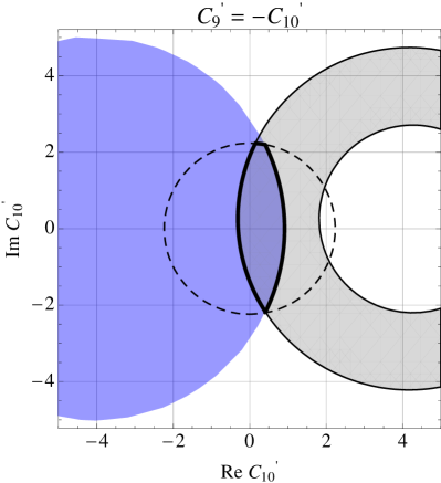
Figure 3: Allowed regions in the complex $C_{10}^{\prime}$ plane in the scenario with $C_{9}^{\prime}=C_{10}^{\prime}$ (upper plot) or with $C_{9}^{\prime}=-C_{10}^{\prime}$ (lower plot). Blue region corresponds to $\mathrm{Br}(B_{s}\to\mu^{+}\mu^{-})$, whereas the gray region and dashed lines mark the $\mathrm{Br}(B\to K\mu^{+}\mu^{-})$ and $B\to X_{s}\mu^{+}\mu^{-}$ constraints, respectively. The intersection of all three constraints is outlined in thick.

VII Conclusion

We have demonstrated in detail that color triplet bosons, i.e., leptoquarks, can generate an entire set of effective operators of $b\to s\ell^{+}\ell^{-}$ processes, including scalar and pseudoscalar ones. There are in total 4 scalar and 3 vector states that contribute to those operators at tree-level. Only two vector, baryon number violating leptoquarks are capable of inducing (pseudo)scalar effective operators that are in general accompanied by vector and axial-vector operators. This feature is simply due to a fact that all scalar leptoquarks that couple to down-type quarks and charged leptons are chiral, namely they can couple either to right- or left-handed leptons. This is not the case for leptoquarks that induce $c\to u\ell^{+}\ell^{-}$ process where a scalar state does lead to scalar and tensor effective operators Fajfer and Kosnik (2009).

Remaining 1 vector and 4 scalar leptoquarks couple to down-type quarks and leptons chirally and their effects are limited to pairs of vector and axial-vector effective operators. We have constrained their Wilson coefficients by imposing the experimental constraints coming from $\mathrm{Br}(B_{s}\to\mu^{+}\mu^{-})$, $\mathrm{Br}(B\to K\ell^{+}\ell^{-})$, and $\mathrm{Br}(B\to X_{s}\mu^{+}\mu^{-})_{[1\mathrm{\leavevmode\nobreak\ GeV}^{2}<q^{2}<6\mathrm{\leavevmode\nobreak\ GeV}^{2}]}$. Importance of individual constraints depends on the particular leptoquark state. The most constraining measurement in almost all cases is the $\mathrm{Br}(B\to K\ell^{+}\ell^{-})$, while $B_{s}\to\mu^{+}\mu^{-}$ is also becoming a sensitive probe of (axial-)vector operators. Presence of these operators can be tested for in transverse asymmetries of $B\to K^{*}\ell^{+}\ell^{-}$ decays as shown in Kruger and Matias (2005); *Becirevic:2011bp; *Matias:2012xw. Finally, all the considered leptoquark states contribute to the electromagnetic Descotes-Genon et al. (2011); *Becirevic:2012dx and chromomagnetic operators of both chiralities, though contributions of this sort involve many more leptoquark couplings and are loop-suppressed compared to the effects studied in this work.

We have found typical allowed values of leptoquark-induced Wilson coefficients are of order $1$, which corresponds to strong constraint $|(g_{L})_{b\ell}(g_{L})_{s\ell}|$, $|(g_{R})_{b\ell}(g_{R})_{s\ell}|\lesssim\textrm{few}\times 10^{-2}$, if leptoquark mass is set to $1\mathrm{\leavevmode\nobreak\ TeV}$. Note that individual $(g_{L,R})_{i\ell}$, $i=s,b$ can still be large and allow for, e.g., explanation of the anomalous muon magnetic moment Dorsner et al. (2011). That very combination of couplings also enters in direct searches for leptoquark pair production. Consequently, final states with either two or no $b$-quark jets are likely to be enhanced with respect to a channel with one $b$-quark jet.

References

• Abazov et al. (2010) V. M. Abazov et al. (D0 Collaboration), Phys.Lett. B693, 539 (2010), eprint 1006.3469.
• Aaltonen et al. (2011) T. Aaltonen et al. (CDF Collaboration), Phys.Rev.Lett. 107, 239903 (2011), eprint 1107.2304.
• Chatrchyan et al. (2011) S. Chatrchyan et al. (CMS Collaboration), Phys.Rev.Lett. 107, 191802 (2011), eprint 1107.5834.
• Aaij et al. (2012a) R. Aaij et al. (LHCb collaboration), Phys. Rev. Lett. 108, 231801 (2012a), eprint 1203.4493.
• Buras (2003) A. J. Buras, Phys.Lett. B566, 115 (2003), eprint hep-ph/0303060.
• Iwasaki et al. (2005) M. Iwasaki et al. (Belle Collaboration), Phys.Rev. D72, 092005 (2005), eprint hep-ex/0503044.
• Aubert et al. (2004) B. Aubert et al. (BABAR Collaboration), Phys. Rev. Lett. 93, 081802 (2004).
• Sun et al. (2012) L. Sun et al. (BABAR Collaboration) (2012), eprint 1204.3933.
• Aaij et al. (2012b) R. Aaij et al. (LHCb Collaboration) (2012b), eprint 1205.3422.
• Alok et al. (2011) A. K. Alok, A. Datta, A. Dighe, M. Duraisamy, D. Ghosh, et al., JHEP 1111, 121 (2011), eprint 1008.2367.
• Drobnak et al. (2012) J. Drobnak, S. Fajfer, and J. F. Kamenik, Nucl.Phys. B855, 82 (2012), eprint 1109.2357.
• Bobeth et al. (2012) C. Bobeth, G. Hiller, D. van Dyk, and C. Wacker, JHEP 1201, 107 (2012), eprint 1111.2558.
• Beaujean et al. (2012) F. Beaujean, C. Bobeth, D. van Dyk, and C. Wacker (2012), eprint 1205.1838.
• Mahmoudi et al. (2012) F. Mahmoudi, S. Neshatpour, and J. Orloff (2012), eprint 1205.1845.
• Altmannshofer and Straub (2012) W. Altmannshofer and D. M. Straub (2012), eprint 1206.0273.
• Becirevic et al. (2012a) D. Becirevic, N. Kosnik, F. Mescia, and E. Schneider (2012a), eprint 1205.5811.
• Kruger and Matias (2005) F. Kruger and J. Matias, Phys.Rev. D71, 094009 (2005), eprint hep-ph/0502060.
• Becirevic and Schneider (2012) D. Becirevic and E. Schneider, Nucl.Phys. B854, 321 (2012), eprint 1106.3283.
• Georgi and Glashow (1974) H. Georgi and S. Glashow, Phys.Rev.Lett. 32, 438 (1974).
• Frampton and Lee (1990) P. H. Frampton and B.-H. Lee, Phys. Rev. Lett. 64, 619 (1990).
• Dorsner and Fileviez Perez (2005) I. Dorsner and P. Fileviez Perez, Nucl.Phys. B723, 53 (2005), eprint hep-ph/0504276.
• Pati and Salam (1974) J. C. Pati and A. Salam, Phys.Rev. D10, 275 (1974).
• Schrempp and Schrempp (1985) B. Schrempp and F. Schrempp, Phys.Lett. B153, 101 (1985).
• Gripaios (2010) B. Gripaios, JHEP 1002, 045 (2010), eprint 0910.1789.
• Kaplan (1991) D. B. Kaplan, Nucl.Phys. B365, 259 (1991).
• Buchmuller et al. (1987) W. Buchmuller, R. Ruckl, and D. Wyler, Phys.Lett. B191, 442 (1987).
• Leurer (1994a) M. Leurer, Phys.Rev. D49, 333 (1994a), eprint hep-ph/9309266.
• Davidson et al. (1994) S. Davidson, D. C. Bailey, and B. A. Campbell, Z.Phys. C61, 613 (1994), eprint hep-ph/9309310.
• Hewett and Rizzo (1997) J. L. Hewett and T. G. Rizzo, Phys. Rev. D 56, 5709 (1997).
• Alikhanov (2012) I. Alikhanov (2012), eprint 1203.3631.
• Saha et al. (2010) J. P. Saha, B. Misra, and A. Kundu, Phys.Rev. D81, 095011 (2010), eprint 1003.1384.
• Dighe et al. (2010) A. Dighe, A. Kundu, and S. Nandi, Phys.Rev. D82, 031502 (2010), eprint 1005.4051.
• Carpentier and Davidson (2010) M. Carpentier and S. Davidson, Eur.Phys.J. C70, 1071 (2010), eprint 1008.0280.
• Bobeth and Haisch (2011) C. Bobeth and U. Haisch (2011), eprint 1109.1826.
• Dorsner et al. (2011) I. Dorsner, J. Drobnak, S. Fajfer, J. F. Kamenik, and N. Kosnik, JHEP 1111, 002 (2011), eprint 1107.5393.
• Grinstein et al. (1989) B. Grinstein, M. J. Savage, and M. B. Wise, Nucl.Phys. B319, 271 (1989).
• Misiak (1993) M. Misiak, Nucl.Phys. B393, 23 (1993).
• Buras and Munz (1995) A. J. Buras and M. Munz, Phys.Rev. D52, 186 (1995), eprint hep-ph/9501281.
• Bobeth et al. (2000) C. Bobeth, M. Misiak, and J. Urban, Nucl.Phys. B574, 291 (2000), eprint hep-ph/9910220.
• Buras et al. (1994) A. Buras, M. Misiak, M. Munz, and S. Pokorski, Nucl.Phys. B424, 374 (1994), eprint hep-ph/9311345.
• Altmannshofer et al. (2009) W. Altmannshofer, P. Ball, A. Bharucha, A. J. Buras, D. M. Straub, et al., JHEP 0901, 019 (2009), eprint 0811.1214.
• Abramowicz et al. (2012) H. Abramowicz et al. (ZEUS Collaboration) (2012), eprint 1205.5179.
• Abazov et al. (2006) V. Abazov et al. (D0 Collaboration), Phys.Lett. B636, 183 (2006), eprint hep-ex/0601047.
• Khachatryan et al. (2011) V. Khachatryan et al. (CMS Collaboration), Phys.Rev.Lett. 106, 201803 (2011), eprint 1012.4033.
• Aad et al. (2012a) G. Aad et al. (ATLAS Collaboration) (2012a), eprint 1203.3172.
• Aad et al. (2012b) G. Aad et al. (ATLAS Collaboration), Phys.Lett. B709, 158 (2012b), eprint 1112.4828.
• Bobeth et al. (2004) C. Bobeth, P. Gambino, M. Gorbahn, and U. Haisch, JHEP 0404, 071 (2004), eprint hep-ph/0312090.
• Logan and Nierste (2000) H. E. Logan and U. Nierste, Nucl.Phys. B586, 39 (2000), eprint hep-ph/0004139.
• Bobeth et al. (2007) C. Bobeth, G. Hiller, and G. Piranishvili, JHEP 0712, 040 (2007), eprint 0709.4174.
• Zhou et al. (2011) R. Zhou et al. (Fermilab Lattice, MILC Collaborations) (2011), eprint 1111.0981.
• Becirevic et al. (in preparation) D. Becirevic et al. (in preparation).
• Ball and Zwicky (2005) P. Ball and R. Zwicky, Phys.Rev. D71, 014029 (2005), eprint hep-ph/0412079.
• Khodjamirian et al. (2007) A. Khodjamirian, T. Mannel, and N. Offen, Phys.Rev. D75, 054013 (2007), eprint hep-ph/0611193.
• Huber et al. (2008) T. Huber, T. Hurth, and E. Lunghi, Nucl.Phys. B802, 40 (2008), eprint 0712.3009.
• Ali et al. (2002) A. Ali, E. Lunghi, C. Greub, and G. Hiller, Phys. Rev. D 66, 034002 (2002).
• Fukae et al. (2000) S. Fukae, C. Kim, and T. Yoshikawa, Phys.Rev. D61, 074015 (2000), eprint hep-ph/9908229.
• Hirsch et al. (1996) M. Hirsch, H. Klapdor-Kleingrothaus, and S. Kovalenko, Phys.Lett. B378, 17 (1996), eprint hep-ph/9602305.
• Aristizabal Sierra et al. (2008) D. Aristizabal Sierra, M. Hirsch, and S. G. Kovalenko, Phys. Rev. D 77, 055011 (2008).
• Leurer (1994b) M. Leurer, Phys.Rev. D50, 536 (1994b), eprint hep-ph/9312341.
• Nath and Fileviez Perez (2007) P. Nath and P. Fileviez Perez, Phys.Rept. 441, 191 (2007), eprint hep-ph/0601023.
• Dorsner et al. (2012) I. Dorsner, S. Fajfer, and N. Kosnik (2012), eprint 1204.0674.
• Fajfer and Kosnik (2009) S. Fajfer and N. Kosnik, Phys.Rev. D79, 017502 (2009), eprint 0810.4858.
• Matias et al. (2012) J. Matias, F. Mescia, M. Ramon, and J. Virto, JHEP 1204, 104 (2012), eprint 1202.4266.
• Descotes-Genon et al. (2011) S. Descotes-Genon, D. Ghosh, J. Matias, and M. Ramon, JHEP 1106, 099 (2011), eprint 1104.3342.
• Becirevic et al. (2012b) D. Becirevic, E. Kou, A. L. Yaouanc, and A. Tayduganov (2012b), eprint 1206.1502.