The higher grading structure of the WKI hierarchy
and the two-component short pulse equation

Abstract

A higher grading affine algebraic construction of integrable hierarchies, containing the Wadati-Konno-Ichikawa (WKI) hierarchy as a particular case, is proposed. We show that a two-component generalization of the Schäfer-Wayne short pulse equation arises quite naturally from the first negative flow of the WKI hierarchy. Some novel integrable nonautonomous models are also proposed. The conserved charges, both local and nonlocal, are obtained from the Riccati form of the spectral problem. The loop-soliton solutions of the WKI hierarchy are systematically constructed through gauge followed by reciprocal Bäcklund transformation, establishing the precise connection between the whole WKI and AKNS hierarchies. The connection between the short pulse equation with the sine-Gordon model is extended to a correspondence between the two-component short pulse equation and the Lund-Regge model.

1 Introduction

The classification of integrable models is of fundamental importance. A systematization in this vein is the graded affine algebraic construction of integrable hierarchies [1, 2], unifying in a single algebraic structure, different models that at first sight appear unrelated. For instance, the modified Korteweg-de Vries (mKdV) and sine/sinh-Gordon models are members of the same hierarchy. Another example is given by the cubic nonlinear Schrödinger (NLS) and the Lund-Regge models, which are members of the Ablowitz-Kaup-Newell-Segur (AKNS) hierarchy. Due to the fact that all the models within a hierarchy share the same algebraic structure, solitonic solutions for all of them can be constructed in a universal manner, through the dressing method [3].

The short pulse equation (SPE)

$$\tfrac{1}{4}u_{xt}=u+\tfrac{1}{6}\left(u^{3}\right)_{xx}$$ (1.1)

was proposed [4] as a model to describe ultra-short optical pulses traversing within a nonlinear media. This equation replaces the standard NLS equation in the ultra-short pulse regime, being a very good approximation of Maxwell’s equations. Since then, (1.1) was proved to be integrable [5] having a Lax pair of the Wadati-Konno-Ichikawa (WKI) type [6]. Moreover, it was shown [5] that (1.1) is related, through a hodograph transformation, to the sine-Gordon equation

$$\theta_{ys}=4\sin\theta$$ (1.2)

from whence its solitary solutions were first obtained [7]. The hodograph transformation was further explored [8] to construct solitonic and quasi-periodic solutions. The transformation connecting (1.1) and (1.2) reads

$$\begin{split}dx&=\alpha dy-2u^{2}dt,\\ dt&=ds,\\ \alpha^{2}&=\left(1+u_{x}^{2}\right)^{-1}=\cos\theta,\\ u&=\tfrac{1}{4}\theta_{s}.\end{split}$$ (1.3)

Through a recursion operator approach, it was proposed in [9] a hierarchy containing (1.1) and also the elastic beam equation (EBE) [10]

$$u_{xt}=\dfrac{1}{4}\left(\dfrac{u_{xx}}{\left(1+u_{x}^{2}\right)^{3/2}}\right)_{xx}.$$ (1.4)

The bi-Hamiltonian structure and nonlocal conservation charges for this single component field hierarchy were also proposed [11]. Recently, a multi-component generalization of the short pulse equation was proposed [12] together with its soliton solutions.

On the other hand, the algebraic construction [1, 2] of integrable hierarchies is based on Toda field theories and the fields appear as coefficients of a linear combination of zero grade operators. This construction was further generalized [13, 14, 15] by the addition of fields associated to higher grading operators, yielding the generalized affine Toda models. The higher grade fields are physically interpreted as matter fields with the usual Toda fields coupled to them.

In this paper, we propose a general higher grading construction for the zero curvature equation, containing the WKI hierarchy as a particular case. In our construction, the zero grade Toda fields are completely removed, remaining the higher grade fields only. Considering the WKI hierarchy, its previous known models appear as members of the positive (time) flows. We then extend the WKI hierarchy to incorporate negative flows, which were not been previously considered. Deriving the first negative flow, a model which is a two-component generalization of the SPE (1.1) emerges quite naturally, showing that the SPE is in fact a natural member of the WKI hierarchy and underlies the same algebraic structure as the previous known models within the positive flows. This two-component short pulse equation (2-SPE) was also introduced recently in [12] under a different context. We also introduce some novel nonautonomous models, mixing a positive flow with a negative one [16]. The conserved charges, both local and nonlocal, are constructed from the Riccati form of the spectral problem [17].

The WKI and AKNS hierarchies are known to be related [18, 19], but this connection was not sufficiently explored. Driven by this results we establish, from an algebraic perspective, the relation between both hierarchies, thus systematizing and extending the hodograph transformation (1.3) for the whole WKI hierarchy. As an example, we explicitly derive a correspondence between the 2-SPE and the Lund-Regge model, where (1.3) appear as a particular case. Our relations also provide explicit and systematic solutions for all the models within the WKI hierarchy in terms of the known AKNS tau functions.

We organize our work as follows. In section 2 we introduce the main algebraic concepts and the usual construction. In section 3, a higher grading integrable hierarchy with an arbitrary affine Lie algebra ${\widehat{\mathcal{G}}}$ is proposed, then, in section 4, this construction yields the WKI hierarchy by choosing ${\widehat{\mathcal{G}}}=\hat{A}_{1}$ with homogeneous gradation. The known models of the WKI hierarchy are derived by considering the positive flows and the 2-SPE emerges from the first negative flow. We also propose some novel nonautonomous integrable models. In section 5, we derive the local and nonlocal conserved charges for the WKI hierarchy. In section 6, we show that the dressing method is unable to solve the WKI hierarchy, then we gauge the AKNS hierarchy into the WKI hierarchy with the aid of a reciprocal Bäcklund transformation, mapping the corresponding flows of both hierarchies. We consider explicitly this mapping between the first negative flows, obtaining a correspondence between the 2-SPE and the Lund-Regge model. Our final remarks are presented in section 7.

2 The usual algebraic construction

Let ${\widehat{\mathcal{G}}}$ be an affine Kac-Moody algebra and $Q$ an operator decomposing the algebra into the graded subspaces

$${\widehat{\mathcal{G}}}=\bigoplus_{j\in\mathbb{Z}}{\widehat{\mathcal{G}}}^{(j)},\qquad\bigl{[}Q,{\widehat{\mathcal{G}}}^{(j)}\bigr{]}=j{\widehat{\mathcal{G}}}^{(j)}.$$ (2.1)

As a consequence of the Jacobi identity, $\bigl{[}{\widehat{\mathcal{G}}}^{(i)},{\widehat{\mathcal{G}}}^{(j)}\bigr{]}\subset{\widehat{\mathcal{G}}}^{(i+j)}$. Let $E$ be a semi-simple element, with a definite grade, defining the kernel subspace

$${\cal K}\equiv\big{\{}T\in{\widehat{\mathcal{G}}}\ |\ \bigl{[}E,T\bigr{]}=0\big{\}}.$$ (2.2)

The image subspace, ${\cal M}$, is its complement and ${\widehat{\mathcal{G}}}={\cal K}\oplus{\cal M}$. Then we have the relations $\bigl{[}{\cal K},{\cal K}\bigr{]}\subset{\cal K}$, $\bigl{[}{\cal K},{\cal M}\bigr{]}\subset{\cal M}$ and we assume the symmetric space structure $\bigl{[}{\cal M},{\cal M}\bigr{]}\subset{\cal K}$.

Integrable hierarchies are constructed from the zero curvature equation

$$\bigl{[}\partial_{x}+U,\partial_{t}+V\bigr{]}=0,$$ (2.3)

where the Lax pair $U$ and $V$ lie on ${\widehat{\mathcal{G}}}$ and have the following form,

$$U\equiv E^{(1)}+A^{(0)}[\phi]$$ (2.4)

where $E=E^{(1)}\in{\widehat{\mathcal{G}}}^{(1)}$ is a constant semi-simple element, defining ${\cal K}$ and ${\cal M}$, and $A^{(0)}[\phi]\in{\cal M}^{(0)}$, where ${\cal M}^{(0)}={\cal M}\cap{\widehat{\mathcal{G}}}^{(0)}$, is the operator containing the fields of the models. For instance, if ${\cal M}^{(0)}$ is spanned by $\big{\{}T^{(0)}_{1},\dotsc,T^{(0)}_{h}\big{\}}$ then $A^{(0)}[\phi]=\phi_{1}T^{(0)}_{1}+\dotsb+\phi_{h}T^{(0)}_{h}$, $\phi_{i}=\phi_{i}\left(x,t\right)$ and $\phi=\left(\phi_{1},\dotsc,\phi_{h}\right)^{T}$. The other Lax operator has the form

$$V \equiv\sum_{i=0}^{n}D^{(i)}\qquad\textnormal{(for positive flows)},$$ (2.5)

$$V \equiv\sum_{i=-n}^{-1}D^{(i)}\qquad\textnormal{(for negative flows)}.$$ (2.6)

The positive integer $n$ labels the (time) flow under quest. Formally, we should have written $V=V\left(n\right)$ and $t=t_{n}$, showing explicitly the flow we are considering, i.e. the particular model within the hierarchy, but we usually omit the index $n$ that will be clearly indicated from the context. It is possible to show that the operators $D^{(i)}\in{\widehat{\mathcal{G}}}^{(i)}$ are determined in terms of the fields contained in $A^{(0)}$ by projecting the zero curvature equation (2.3) into each graded subspace according to (2.1). This procedure enables us to construct the operator $V$, one for each flow $n$, in terms of the algebraic structure of the operator $U$, thus yielding a nonlinear model together with its Lax pair. Therefore, by construction, all the models are immediately classified through $\langle{\widehat{\mathcal{G}}},Q,E^{(1)}\rangle$, defining an integrable hierarchy of differential equations.

3 A higher grading construction

We now propose a higher grading construction without the usual Toda fields, keeping the higher grade fields only. Let us define the following zero curvature Lax pair

$$U \equiv E^{(1)}+A^{(1)}[\phi],$$ (3.1a)

$$V \equiv\sum_{i=-m}^{n}D^{(i)}[\phi],$$ (3.1b)

where $E=E^{(1)}\in{\widehat{\mathcal{G}}}^{(1)}$ is a constant semi-simple element and $A^{(1)}[\phi]\in{\cal M}^{(1)}$, where ${\cal M}^{(1)}={\cal M}\cap{\widehat{\mathcal{G}}}^{(1)}$, is the operator containing the fields now having grade one. The positive integers $n$ and $m$ label each model, mixing a positive flow $n$ with a negative flow $m$ [16]. To study positive and negative flows separately one should consider

$$V \equiv\sum_{i=1}^{n}D^{(i)}\qquad\text{(for positive flows)},$$ (3.2)

$$V \equiv\sum_{i=-n}^{1}D^{(i)}\qquad\text{(for negative flows)}.$$ (3.3)

With this algebraic structure, the zero curvature equation can be solved non trivially in the following way. Taking (2.3) with (3.1), the projection into each graded subspace yields the following set of equations

$$\begin{split}\bigl{[}E^{(1)}+A^{(1)},D^{(n)}\bigr{]}&=0\qquad\text{grade $n+1$},\\ \partial_{x}D^{(n)}+\bigl{[}E^{(1)}+A^{(1)},D^{(n-1)}\bigr{]}&=0\qquad\text{grade $n$},\\ &\ \,\vdots\\ \partial_{x}D^{(1)}-\partial_{t}A^{(1)}+\bigl{[}E^{(1)}+A^{(1)},D^{(0)}\bigr{]}&=0\qquad\text{grade $1$},\\ &\ \,\vdots\\ \partial_{x}D^{(-m+1)}+\bigl{[}E^{(1)}+A^{(1)},D^{(-m)}\bigr{]}&=0\qquad\text{grade $-m+1$},\\ \partial_{x}D^{(-m)}&=0\qquad\text{grade $-m$}.\end{split}$$ (3.4)

Note that the equations of motion comes from the projection into ${\cal M}\cap{\widehat{\mathcal{G}}}^{(1)}$. Each equation is further decomposed into ${\cal K}$ and ${\cal M}$ components. For mixed or negative flows, we have the equations of motion in the following form

$$\partial_{t}A^{(1)}=\partial_{x}D^{(1)}_{{\cal M}}+\bigl{[}E^{(1)},D^{(0)}_{{\cal M}}\bigr{]}+\bigl{[}A^{(1)},D^{(0)}_{{\cal K}}\bigr{]},$$ (3.5)

while for positive flows the equations of motion are given by

$$\partial_{t}A^{(1)}=\partial_{x}D^{(1)}_{{\cal M}},$$ (3.6)

where $D^{(j)}=D^{(j)}_{{\cal K}}+D^{(j)}_{{\cal M}}$. We remark that this construction is valid for an arbitrary affine Lie algebra ${\widehat{\mathcal{G}}}$ with a grading operator $Q$ and arbitrary grade one semi-simple element $E^{(1)}$.

4 The Wadati-Konno-Ichikawa hierarchy

Let us now consider the Kac-Moody algebra $\hat{A}_{1}=\big{\{}H^{j},E_{+}^{j},E_{-}^{j},\hat{c},\hat{d}\big{\}}$, where $j$ is an integer, with commutation relations given by

$$\begin{split}&\bigl{[}H^{k},H^{j}\bigr{]}=2k\delta_{k+j,0}\hat{c},\quad\bigl{[}H^{k},E_{\pm}^{j}\bigr{]}=\pm 2E_{\pm}^{k+j},\quad\bigl{[}E_{+}^{k},E_{-}^{j}\bigr{]}=H^{k+j}+k\delta_{k+j,0}\hat{c},\\ &\bigl{[}\hat{d},T^{j}\bigr{]}=jT^{j},\quad\bigl{[}\hat{c},T^{j}\bigr{]}=0,\quad\text{where}\quad T^{j}\in\left\{H^{j},\,E_{+}^{j},\,E_{-}^{j}\right\}.\end{split}$$ (4.1)

In the construction of integrable models we use the loop algebra only, achieved by setting $\hat{c}=0$. The homogeneous gradation $Q=\hat{d}$ yields the grading subspaces

$${\widehat{\mathcal{G}}}^{(j)}=\left\{H^{j},E_{+}^{j},E_{-}^{j}\right\}.$$ (4.2)

Let us fix the semi-simple element as $E^{(1)}\equiv H^{1}$, yielding ${\cal K}^{(j)}=\left\{H^{j}\right\}$ and ${\cal M}^{(j)}=\left\{E_{+}^{j},\,E_{-}^{j}\right\}$. Therefore, the operator containing the fields must have the form

$$A^{(1)}=q(x,t)E_{+}^{1}+r(x,t)E_{-}^{1},$$ (4.3)

where $q$ and $r$ are both fields of the models. The Lax operator $V$ in (3.1b) is a sum of elements in the form $D^{(j)}=a_{j}E_{+}^{j}+b_{j}E_{-}^{j}+c_{j}H^{j}$, whose coefficients will be determined in terms of $q$ and $r$ by solving the zero curvature equation as described in (3.4).

4.1 Positive flows

The positive flows (3.2) are constructed from the zero curvature equation

$$\bigl{[}\partial_{x}+H^{1}+qE_{+}^{1}+rE_{-}^{1},\partial_{t}+D^{(n)}+D^{(n-1)}+\dotsb+D^{(1)}\bigr{]}=0.$$ (4.4)

Now let us consider the first models.

$\mathbf{n=1}$.

Yields the trivial equations $q_{t}=q_{x}$ and $r_{t}=r_{x}$.

$\mathbf{n=2}$.

Starting from the ${\widehat{\mathcal{G}}}^{(3)}$ projection we have $a_{2}=c_{2}q$ and $b_{2}=c_{2}r$. The ${\widehat{\mathcal{G}}}^{(2)}$ projection gives

$$a_{1}=c_{1}q-\tfrac{1}{2}\partial_{x}a_{2},\qquad b_{1}=c_{1}r+\tfrac{1}{2}\partial_{x}b_{2},\qquad\partial_{x}c_{2}=ra_{1}-qb_{1},$$ (4.5)

from which we have

$$\partial_{x}\ln c_{2}=-\tfrac{1}{2}\partial_{x}\ln\left(1+qr\right),\qquad c_{2}=\left(1+qr\right)^{-1/2}.$$ (4.6)

The ${\cal K}$ component of the ${\widehat{\mathcal{G}}}^{(1)}$ projection implies $\partial_{x}c_{1}=0$. Choosing $c_{1}=0$ the ${\cal M}$ component yields the following equations of motion

$$\partial_{t}q+\partial_{x}^{2}\left(\dfrac{q}{2\left(1+qr\right)^{1/2}}\right)=0,\qquad\partial_{t}r-\partial_{x}^{2}\left(\dfrac{r}{2\left(1+qr\right)^{1/2}}\right)=0.$$ (4.7)

From the coefficients $a_{i}$, $b_{i}$ and $c_{i}$ just found we have the explicit Lax pair for this model which reads

$$U =H^{1}+qE_{+}^{1}+rE_{-}^{1},$$ (4.8a)

$$V =\dfrac{q}{\left(1+qr\right)^{1/2}}E_{+}^{2}+\dfrac{r}{\left(1+qr\right)^{1/2}}E_{-}^{2}+\dfrac{1}{\left(1+qr\right)^{1/2}}H^{2}$$

$$\qquad-\partial_{x}\left(\dfrac{q}{2\left(1+qr\right)^{1/2}}\right)E_{+}^{1}+\partial_{x}\left(\dfrac{r}{2\left(1+qr\right)^{1/2}}\right)E_{-}^{1}.$$ (4.8b)

The choice $r=q^{*}$, $x\to ix$ and $t\to 2it$ reduces (4.7) to the Wadati-Konno-Ichikawa-Shimizu equation [20]

$$i\partial_{t}q+\partial_{x}^{2}\left(\frac{q}{\left(1+|q|^{2}\right)^{1/2}}\right)=0.$$ (4.9)

$\mathbf{n=3}$.

In this case we get the following model

$$\partial_{t}q-\partial_{x}^{2}\left(\dfrac{q_{x}}{4\left(1+qr\right)^{3/2}}\right)=0,\qquad\partial_{t}r-\partial_{x}^{2}\left(\dfrac{r_{x}}{4\left(1+qr\right)^{3/2}}\right)=0,$$ (4.10)

whose Lax pair is

$$U =H^{1}+qE_{+}^{1}+rE_{-}^{1},$$ (4.11a)

$$V =\frac{q}{\left(1+qr\right)^{1/2}}E_{+}^{3}+\frac{r}{\left(1+qr\right)^{1/2}}E_{-}^{3}+\frac{1}{\left(1+qr\right)^{1/2}}H^{3}$$

$$\qquad-\dfrac{q_{x}}{2\left(1+qr\right)^{3/2}}E_{+}^{2}+\dfrac{r_{x}}{2\left(1+qr\right)^{3/2}}E_{-}^{2}+\dfrac{q_{x}r-qr_{x}}{4\left(1+qr\right)^{3/2}}H^{2}$$

$$\qquad+\partial_{x}\left(\dfrac{q_{x}}{4\left(1+qr\right)^{3/2}}\right)E_{+}^{1}+\partial_{x}\left(\dfrac{r_{x}}{4\left(1+qr\right)^{3/2}}\right)E_{-}^{1}.$$ (4.11b)

Choosing $r=q$ and $t\to-4t$ the model (4.10) becomes

$$\partial_{t}q+\partial_{x}^{2}\left(\frac{q_{x}}{\left(1+q^{2}\right)^{3/2}}\right)=0,$$ (4.12)

which is the EBE (1.4). Note also that, by choosing $r=1$, $q=v-1$ and $t\to-2t$, the system (4.10) is transformed into the Dym equation

$$v_{t}=\left(v^{-1/2}\right)_{xxx}.$$ (4.13)

The Lax pair for the Dym equation, and also for (4.12), are obtained from (4.11) as particular cases. The models (4.7) and (4.10) were proposed in [6] and are the first members of the positive WKI hierarchy.

4.2 Negative flows

We now extend the WKI hierarchy to incorporate negative flows. According to our construction, the negative flows are generated using the operator (3.3) yielding

$$\bigl{[}\partial_{x}+H^{1}+qE_{+}^{1}+rE_{-}^{1},\partial_{t}+D^{(-n)}+D^{(-n+1)}+\dotsb+D^{(0)}+D^{(1)}\bigr{]}=0.$$ (4.14)

$\mathbf{n=1}$.

The projection into ${\widehat{\mathcal{G}}}^{(-1)}$ implies that $a_{-1},\;b_{-1}$ and $c_{-1}$ are all constants. The ${\widehat{\mathcal{G}}}^{(0)}$ projection yields

$$\partial_{x}a_{0}=2c_{-1}q-2a_{-1},\qquad\partial_{x}b_{0}=-2c_{-1}r+2b_{-1},\qquad\partial_{x}c_{0}=a_{-1}r-b_{-1}q.$$ (4.15)

Let us introduce the operator

$$\partial_{x}^{-1}f(x)\equiv\int_{-\infty}^{x}f(y)dy.$$ (4.16)

We assume that the fields and its derivatives of any order decay sufficiently fast when $|x|\to\infty$. Under this condition $\partial_{x}\partial_{x}^{-1}f(x)=\partial_{x}^{-1}\partial_{x}f(x)=f(x)$.

To eliminate an explicit $x$ dependence in (4.15) we set $a_{-1}=b_{-1}=0$ thus

$$a_{0}=2c_{-1}\partial_{x}^{-1}q,\qquad b_{0}=-2c_{-1}\partial_{x}^{-1}r,\qquad c_{0}=\text{const.}$$ (4.17)

The projection into ${\widehat{\mathcal{G}}}^{(2)}$ implies that $a_{1}=c_{1}q$ and $b_{1}=c_{1}r$. The ${\widehat{\mathcal{G}}}^{(1)}$ projection yields the field equations plus one constraint

$$\partial_{t}q=\partial_{x}a_{1}+2a_{0}-2c_{0}q,\qquad\partial_{t}r=\partial_{x}b_{1}-2b_{0}+2c_{0}r,\qquad\partial_{x}c_{1}=a_{0}r-b_{0}q.$$ (4.18)

From this last equation and (4.17) we have

$$c_{1}=2c_{-1}\partial_{x}^{-1}\left(r\partial_{x}^{-1}q+q\partial_{x}^{-1}r\right).$$ (4.19)

Choosing $c_{0}=0$ and fixing $c_{-1}=1$, we obtain the nonlocal equations of motion

$$\partial_{t}q =4\partial_{x}^{-1}q+2\partial_{x}\left(q\partial_{x}^{-1}\left(r\partial_{x}^{-1}q+q\partial_{x}^{-1}r\right)\right),$$ (4.20a)

$$\partial_{t}r =4\partial_{x}^{-1}r+2\partial_{x}\left(r\partial_{x}^{-1}\left(r\partial_{x}^{-1}q+q\partial_{x}^{-1}r\right)\right).$$ (4.20b)

Introducing the new fields defined by

$$q\equiv\partial_{x}u,\qquad r\equiv\partial_{x}v,$$ (4.21)

we can write (4.20) in a local form yielding

$$u_{xt} =4u+2\partial_{x}\left(uvu_{x}\right),$$ (4.22a)

$$v_{xt} =4v+2\partial_{x}\left(uvv_{x}\right).$$ (4.22b)

This model was also proposed recently in [12]. Note that (4.22) is symmetric by the interchange of $u$ and $v$ and invariant under the following transformations

$$x\to\mu x,\qquad t\to\mu^{-1}t,\qquad u\to\mu^{n}u,\qquad v\to\mu^{2-n}v,$$ (4.23)

for a constant $\mu$. The explicit Lax pair of model (4.22) is given by

$$U =H^{1}+u_{x}E_{+}^{1}+v_{x}E_{-}^{1},$$ (4.24a)

$$V =H^{-1}+2uE_{+}^{0}-2vE_{-}^{0}+2uvH^{1}+2uvu_{x}E_{+}^{1}+2uvv_{x}E_{-}^{1}.$$ (4.24b)

If we reduce the model (4.22) to a single component field by choosing $v=u$, we have the SPE (1.1)

$$\tfrac{1}{4}u_{xt}=u+\tfrac{1}{6}\left(u^{3}\right)_{xx}.$$ (4.25)

Therefore, the model (4.22) is a two-component generalization of the SPE and a natural member of the WKI hierarchy, sharing the same algebraic structure as the previous known models within the positive flows. A $n$-component generalization of the SPE, following the structure of (4.22), was also proposed in [12] and our construction strongly suggests that it can be obtained by considering the untwisted algebra $\hat{A}_{n-1}\sim\hat{s\ell}(n)$, which will also generate $n$-component extensions of (4.9) and (4.12).

$\mathbf{n=2}$.

Setting $c_{-2}=b_{-2}=0$ to eliminate explicit $x$ dependencies and introducing new fields defined through $q\equiv u_{xx}$ and $r\equiv v_{xx}$, we get the following model

$$u_{xxt} =2a\left\{2u_{x}+\partial_{x}\left(u_{x}v_{x}u_{xx}\right)\right\}$$

$$\qquad-4b\left\{2u+u_{x}v_{x}u_{xx}+\partial_{x}\left(u_{xx}\left(uv_{x}-vu_{x}\right)\right)\right\},$$ (4.26a)

$$v_{xxt} =2a\left\{2v_{x}+\partial_{x}\left(u_{x}v_{x}v_{xx}\right)\right\}$$

$$\qquad+4b\left\{2v+u_{x}v_{x}v_{xx}-\partial_{x}\left(v_{xx}\left(uv_{x}-vu_{x}\right)\right)\right\},$$ (4.26b)

where $a\equiv c_{-1}$ and $b\equiv c_{-2}$ are constants. The Lax pair for this model is

$$U =H^{1}+u_{xx}E_{+}^{1}+v_{xx}E_{-}^{1},$$ (4.27a)

$$V =bH^{-2}+2bu_{x}E_{+}^{-1}-2bv_{x}E_{-}^{-1}+aH^{-1}$$

$$\qquad+2\left(au_{x}-2bu\right)E_{+}^{0}-2\left(av_{x}+2bv\right)E_{-}^{0}+2bu_{x}v_{x}H^{0}$$

$$\qquad+2u_{xx}\left(au_{x}v_{x}-2b\left(uv_{x}-vu_{x}\right)\right)E_{+}^{1}+2v_{xx}\left(au_{x}v_{x}-2b\left(uv_{x}-vu_{x}\right)\right)E_{-}^{1}$$

$$\qquad+2\left(au_{x}v_{x}-2b\left(uv_{x}-vu_{x}\right)\right)H^{1}.$$ (4.27b)

Note that the term next to the $a$ coefficient in (4.26) is the system (4.22). Setting $a=0$ and $b=\tfrac{1}{4}$ we have

$$\left(u_{xt}+u_{xx}\left(uv_{x}-vu_{x}\right)\right)_{x} =-2u-u_{x}v_{x}u_{xx},$$ (4.28a)

$$\left(v_{xt}+v_{xx}\left(uv_{x}-vu_{x}\right)\right)_{x} =2v+u_{x}v_{x}v_{xx},$$ (4.28b)

which after the substitution $v=u^{*}$ and $t\to it$ becomes the single equation

$$\left(iu_{xt}+u_{xx}\left(u^{*}u_{x}-uu^{*}_{x}\right)\right)_{x}=2u+u_{x}u^{*}_{x}u_{xx}.$$ (4.29)

4.3 Small amplitude limit

Let us give a physical motivation by considering a small amplitude limit. Consider the reduced second positive flow (4.9). Assuming that $q$ is small we have

$$\left(1+|q|^{2}\right)^{-1/2}=1-\dfrac{1}{2}|q|^{2}+\dotsm$$ (4.30)

and then (4.9) becomes

$$iq_{t}+q_{xx}-\tfrac{1}{2}\partial_{x}^{2}\left(|q|^{2}q\right)+\mathcal{O}\left(q^{5}\right)=0.$$ (4.31)

Consider a standard multiple scale expansion ($\epsilon\ll 1$)

$$q=\sum_{n=1}^{\infty}\epsilon^{n}q_{n}(x_{0},t_{0},x_{1},t_{1},\dotsc),\qquad x_{i}=\epsilon^{n}x,\qquad t_{i}=\epsilon^{n}t.$$ (4.32)

Taking order of $\epsilon$ in (4.31) we obtain the plain wave solution

$$q_{1}=Ae^{i\sigma}+A^{*}e^{-i\sigma},\qquad\sigma=\kappa x_{0}-\kappa^{2}t_{0},\qquad A=A(x_{1},t_{1},\dotsc).$$ (4.33)

Taking order of $\epsilon^{2}$, the elimination of the secularity requires that $A=A(x_{1}-2\kappa t_{1},x_{2},t_{2},\dotsc)$ and we choose $q_{2}=0$. Finally, the lower nonlinear contribution comes from the order of $\epsilon^{3}$ and after changing to a coordinate system moving with the envelope $A$, $\xi_{i}\equiv x_{i}-2\kappa t_{i}$ and $\tau_{i}\equiv t_{i}$, we obtain the NLS equation

$$i\partial_{\tau_{2}}A+\partial^{2}_{\xi_{1}}A+\dfrac{3\kappa^{2}}{2}|A|^{2}A=0.$$ (4.34)

Up to this order the small amplitude solution reads

$$q=\epsilon\left(Ae^{i\sigma}+A^{*}e^{-i\sigma}\right)+\epsilon^{3}\left(Be^{3i\sigma}+B^{*}e^{-3i\sigma}\right)+\mathcal{O}\left(\epsilon^{4}\right),$$ (4.35)

where $A$ is determined from (4.34) and contains a nonlinear contribution, and $B$ comes from higher order terms. The positive flows of the WKI hierarchy contain a strong nonlinearity and describes large amplitude solutions, which in the small amplitude limit recover the behaviour described by the AKNS models, like the NLS equation. Due to the large amplitude solutions these models may be of particular interest in nonlinear optics, plasmas, Bose-Einstein condensates and water waves.

Performing the same procedure for the EBE (4.12), the order of $\epsilon$ gives the linear wave (4.33) with $\sigma=\kappa x_{0}+\kappa^{3}t_{0}$. The order of $\epsilon^{2}$ implies $A=A\left(x_{1}+3\kappa^{2}t_{1},x_{2},t_{2},\dotsc\right)$ and $q_{2}=0$. The order of $\epsilon^{3}$, after changing to a coordinate system $\xi_{i}\equiv x_{i}+3\kappa^{2}t_{i}$ and $\tau_{i}\equiv t_{i}$, gives again the NLS equation

$$i\partial_{\tau_{2}}A-3\kappa\partial_{\xi_{1}}^{2}A-3\kappa^{3}|A|^{2}A=0.$$ (4.36)

Consider the SPE (4.25). The $\epsilon$ order gives a linear wave $u_{1}$ having the same form as (4.33) with $\sigma=\kappa x_{0}-4\kappa^{-1}t_{0}$. The $\epsilon^{2}$ order implies $A=A\left(x_{1}+4\kappa^{-2}t_{1},x_{2},t_{2},\dotsc\right)$ and $u_{2}=0$. The $\epsilon^{3}$ order, in the coordinates $\xi_{i}\equiv x_{i}+4\kappa^{-2}t_{i}$ and $\tau_{i}\equiv t_{i}$, gives

$$i\partial_{\tau_{2}}A+4\kappa^{-3}\partial_{\xi_{1}}^{2}A+2\kappa|A|^{2}A=0.$$ (4.37)

Note that the sine-Gordon equation $u_{xt}=\sin u\approx u-\tfrac{1}{6}u^{3}+\dotsb$ has stronger nonlinearities than the short pulse equation, but up to order $\epsilon^{3}$ both of them yields qualitatively the same multiple scale approximation. Contrary to the positive flows of the WKI hierarchy, the short pulse equation does not seem do describe large amplitude solutions.

4.4 Mixed flows

It is possible to combine a positive flow $n$ with a negative flow $m$ by considering the operator (3.1b). Let $n=2$ and $m=1$, leading to the zero curvature equation

$$\bigl{[}\partial_{x}+H^{1}+qE_{+}^{1}+rE_{-}^{1},\partial_{t}+D^{(2)}+D^{(1)}+D^{(0)}+D^{(-1)}\bigr{]}=0.$$ (4.38)

We solve each grade projection starting from highest to lowest, exactly as before, the only modification is that we can let some coefficients, that were previously considered constants, now to depend on $t$, thus providing the nonautonomous ingredient. For individual flows these coefficients were not interesting because they come as a global factor in the final equation. Therefore, after solving (4.38) we obtain

$$u_{xt} =-\dfrac{a(t)}{2}\partial_{x}^{2}\left(\dfrac{u_{x}}{\left(1+u_{x}v_{x}\right)^{1/2}}\right)+4b(t)\left(u+\dfrac{1}{2}\partial_{x}\left(uvu_{x}\right)\right),$$ (4.39a)

$$v_{xt} =+\dfrac{a(t)}{2}\partial_{x}^{2}\left(\dfrac{v_{x}}{\left(1+u_{x}v_{x}\right)^{1/2}}\right)+4b(t)\left(v+\dfrac{1}{2}\partial_{x}\left(uvv_{x}\right)\right),$$ (4.39b)

where $a(t)$ and $b(t)$ are arbitrary functions. Its Lax pair given by

$$U =H^{1}+u_{x}E_{+}^{1}+v_{x}E_{-}^{1},$$ (4.40a)

$$V =a(t)V(+2)+b(t)V(-1),$$ (4.40b)

where $V(+2)$ stands for the operator corresponding to the second positive flow (4.8b), with $q=u_{x}$ and $r=v_{x}$, and $V(-1)$ is (4.24b). Model (4.39) is a nonautonomous mixture of (4.7) and (4.22). This model also admits the reduction $v=u^{*}$, $t\to it$ and $x\to ix$, yielding

$$u_{xt}=\dfrac{ia(t)}{2}\partial_{x}^{2}\left(\dfrac{u_{x}}{\left(1-|u_{x}|^{2}\right)^{1/2}}\right)-4b(t)\left(u-\dfrac{1}{2}\partial_{x}\left(|u|^{2}u_{x}\right)\right).$$ (4.41)

In the same way, for $n=3$ and $m=1$, we have

$$u_{xt} =\dfrac{a(t)}{4}\partial_{x}^{2}\left(\dfrac{u_{xx}}{\left(1+u_{x}v_{x}\right)^{3/2}}\right)+4b(t)\left(u+\dfrac{1}{2}\partial_{x}\left(uvu_{x}\right)\right),$$ (4.42a)

$$v_{xt} =\dfrac{a(t)}{4}\partial_{x}^{2}\left(\dfrac{v_{xx}}{\left(1+u_{x}v_{x}\right)^{3/2}}\right)+4b(t)\left(v+\dfrac{1}{2}\partial_{x}\left(uvv_{x}\right)\right),$$ (4.42b)

together with its Lax pair

$$U =H^{1}+u_{x}E_{+}^{1}+v_{x}E_{-}^{1},$$ (4.43a)

$$V =a(t)V(+3)+b(t)V(-1).$$ (4.43b)

Choosing $v=u$, (4.42) leads to a combination of EBE and SPE

$$u_{xt}=\dfrac{a(t)}{4}\partial_{x}^{2}\left(\dfrac{u_{xx}}{\left(1+(u_{x})^{2}\right)^{3/2}}\right)+4b(t)\left(u+\dfrac{1}{6}\left(u^{3}\right)_{xx}\right).$$ (4.44)

It is possible to combine any positive flow with a negative one, generating nonautonomous models inside the hierarchy. Due to $a(t)$ and $b(t)$ the dispersion relation will have a time depend velocity and the solitons will accelerate. This models may be nice candidates in applications having accelerated ultra-short optical pulses [22].

5 Conservation laws

Consider the linear spectral problem associated to the WKI hierarchy

$$\left(\partial_{x}+U\right)\Psi=0,\qquad\left(\partial_{t}+V\right)\Psi=0,$$ (5.1)

where $U=H^{1}+qE_{+}^{1}+rE_{-}^{1}$ and $V$ depends on the particular flow. Using a matrix representation we have

$$U=\begin{pmatrix}\lambda&\lambda q\\ \lambda r&-\lambda\end{pmatrix},\qquad V=\begin{pmatrix}V_{11}(\lambda)&V_{12}(\lambda)\\ V_{21}(\lambda)&V_{22}(\lambda)\end{pmatrix},\qquad\Psi=\begin{pmatrix}\psi_{1}\\ \psi_{2}\end{pmatrix},$$ (5.2)

where $\lambda$ is the loop algebra spectral parameter. From (5.1) we write the Riccati form of the spectral problem [17], whose compatibility yields the conservation laws

$$\partial_{t}\left(q\Gamma\right)-\partial_{x}\left(\lambda^{-1}\left(V_{11}+V_{12}\Gamma\right)\right) =0,$$ (5.3)

$$\partial_{t}\left(r\Gamma^{-1}\right)-\partial_{x}\left(\lambda^{-1}\left(V_{22}+V_{21}\Gamma^{-1}\right)\right) =0,$$ (5.4)

where we have defined

$$\Gamma\equiv\dfrac{\psi_{2}}{\psi_{1}}.$$ (5.5)

Therefore, we can use $q\Gamma$ and $r\Gamma^{-1}$ to construct an infinite number of conserved charges assuming a power series in $\lambda$. Deriving $\Gamma$ and $\Gamma^{-1}$ with respect to $x$ and writing the result in terms of $F\equiv q\Gamma$ and $G\equiv r\Gamma^{-1}$, we obtain the Riccati equations

$$q\partial_{x}\left(\dfrac{F}{q}\right)+\lambda qr-2\lambda F-\lambda F^{2} =0,$$ (5.6)

$$r\partial_{x}\left(\dfrac{G}{r}\right)+\lambda qr+2\lambda G-\lambda G^{2} =0,$$ (5.7)

which are the generating equations for the conserved densities. Both equations lead to the same results, the densities obtained from (5.7) are the same as those from (5.6) with the interchange $q\leftrightarrow r$, so we will focus on (5.6) only.

5.1 Local charges

Let us consider the expansion

$$F=\sum_{n=0}^{\infty}f_{n}\lambda^{-n}.$$ (5.8)

Substituting (5.8) into (5.6) and taking powers of $\lambda$ we determine each $f_{n}$ recursively, the first ones are given by

$$f_{0} =-1+\left(1+qr\right)^{1/2},$$ (5.9)

$$f_{1} =-\dfrac{1}{2}\partial_{x}\ln\left(\dfrac{q}{\left(1+qr\right)^{1/2}}\right)+\dfrac{q_{x}}{2q\left(1+qr\right)^{1/2}},$$ (5.10)

$$\ \,\vdots$$

The charges associated to these densities, which are conserved thanks to (5.3), are

$$H_{0} =\int_{-\infty}^{\infty}\left(1+qr\right)^{1/2}dx,$$ (5.11)

$$H_{1} =\int_{-\infty}^{\infty}\dfrac{q_{x}}{2q\left(1+qr\right)^{1/2}}dx,$$ (5.12)

$$\ \,\vdots$$

These charges coincide with those in [6] and are the Hamiltonians generating the models within the positive flows.

5.2 Nonlocal charges

The most general expansion compatible with the Riccati equation (5.6), able to generate nonlocal densities, is given by

$$F=\sum_{n=-1}^{\infty}f_{-n}\lambda^{n}.$$ (5.13)

Substituting (5.13) into (5.6) and taking the lowest order, $\lambda^{-1}$, we obtain the Bernoulli differential equation

$$\partial_{x}f_{1}-\left(\partial_{x}\ln q\right)f_{1}=f_{1}^{2},$$ (5.14)

whose solution is

$$f_{1}=-\partial_{x}\ln\left(\partial_{x}^{-1}q\right).$$ (5.15)

Note that it is a total derivative and therefore contributes with a trivial charge. The next orders in $\lambda$ yield the following equations

$$\partial_{x}f_{0}-\left(\partial_{x}\ln q+2f_{1}\right)f_{0} =2f_{1},$$ (5.16)

$$\partial_{x}f_{-1}-\left(\partial_{x}\ln q+2f_{1}\right)f_{-1} =f_{0}^{2}+2f_{0}-qr,$$ (5.17)

$$\partial_{x}f_{-2}-\left(\partial_{x}\ln q+2f_{1}\right)f_{-2} =2f_{0}f_{-1}+2f_{-1},$$ (5.18)

$$\partial_{x}f_{-3}-\left(\partial_{x}\ln q+2f_{1}\right)f_{-3} =f_{-1}^{2}+2f_{0}f_{-2}+2f_{-2},$$ (5.19)

$$\ \,\vdots$$

Integrating (5.16) we obtain

$$f_{0}=2\partial_{x}\left(\dfrac{\partial_{x}^{-2}q}{\partial_{x}^{-1}q}\right)-2,$$ (5.20)

which again generates a trivial charge. From (5.17) we have

$$f_{-1}=\dfrac{q}{\left(\partial_{x}^{-1}q\right)^{2}}\left[4\partial_{x}^{-1}\left(q\left(\dfrac{\partial_{x}^{-2}q}{\partial_{x}^{-1}q}\right)^{2}\right)-4\partial_{x}^{-3}q-\partial_{x}^{-1}\left(r\left(\partial_{x}^{-1}q\right)^{2}\right)\right],$$ (5.21)

which is extremely nonlocal and the next densities becomes even more cumbersome. At this point we should mention that there is in fact three sets of nonlocal charges. The first set of charges comes from continuing this procedure, integrating (5.18) and so on. The second set of charges comes from choosing a trivial solution of the Bernoulli equation, $f_{1}=0$, and the solution $f_{0}=q$ of (5.16). The third set of charges comes from the trivial choices $f_{1}=0$ and $f_{0}=0$. All the subsequent densities are determined by the initial choices of $f_{1}$ and $f_{0}$. Therefore, let $f_{1}=0$ and $f_{0}=q$, then we have

$$f_{0} =q,$$ (5.22)

$$f_{-1} =q\partial_{x}^{-1}\left(q-r+2\right),$$ (5.23)

$$f_{-2} =2q\partial_{x}^{-1}\left((1+q)\partial_{x}^{-1}(q-r+2)\right),$$ (5.24)

$$f_{-3} =q\partial_{x}^{-1}\left(q\left(\partial_{x}^{-1}(q-r+2)\right)^{2}\right)$$

$$\qquad+4q\partial_{x}^{-1}\left((1+q)\partial_{x}^{-1}\left((1+q)\partial_{x}^{-1}(q-r+2)\right)\right),$$ (5.25)

$$\ \,\vdots$$

Let $f_{1}=0$ and $f_{0}=0$, then

$$f_{-1} =-q\partial_{x}^{-1}r,$$ (5.26)

$$f_{-2} =-2q\partial_{x}^{-2}r,$$ (5.27)

$$f_{-3} =-4q\partial_{x}^{-3}r+q\partial_{x}^{-1}\left(q\left(\partial_{x}^{-1}r\right)^{2}\right),$$ (5.28)

$$\ \,\vdots$$

The respective conserved charges are given by

$$H_{-n}=\int_{-\infty}^{\infty}f_{-n}dx,\qquad n=1,2,3,\dotsc$$ (5.29)

Let us emphasize that the charges are conserved for the whole hierarchy of equations, as can be explicitly checked for some of the individual models, either from the positive or negative flows.

6 Gauge and reciprocal transformations

It was proved [4] that (4.25) does not have real valued, smooth, soliton like solutions in the form $u=u(x+ct)$. The models within the WKI hierarchy possess the loop-soliton kind of solutions, and in this section we aim to explain the algebraic origin of this peculiarity.

6.1 Dressing method

First of all, we will show that the dressing method [3], well known to construct soliton solutions of integrable hierarchies, is unable to solve the WKI hierarchy.

The dressing method reconstructs the general operator $U=E^{(1)}+A^{(0)}[\phi]$ by gauging a vacuum solution $U_{0}=E^{(1)}$, corresponding to the trivial field configuration $\phi=0$. There must exist two dressing operators $\Theta_{\pm}$ effecting the following gauge transformations

$$U=\Theta_{\pm}U_{0}\Theta_{\pm}^{-1}-\left(\partial_{x}\Theta_{\pm}\right)\Theta_{\pm}^{-1}.$$ (6.1)

From (5.1) we see that there is a gauge freedom for the operator $U=-\left(\partial_{x}\Psi\right)\Psi^{-1}$, i.e. $\Psi\mapsto\Psi h$ where $h$ is a constant group element. Consider the spectral problem for the vacuum $\left(\partial_{x}+U_{0}\right)\Psi_{0}=0$. Then, the transformations $\Psi_{0}\mapsto\Theta_{+}\Psi_{0}$ and $\Psi_{0}\mapsto\Theta_{-}\Psi_{0}$ will reconstruct the same operator $U$ if they are gauge equivalent, i.e. $\Theta_{+}\Psi_{0}=\Theta_{-}\Psi_{0}h$. In other words, the relations (6.1) are valid, if and only if, the dressing operators are related through a Riemann-Hilbert problem

$$\Theta_{-}^{-1}\Theta_{+}=\Psi_{0}h\Psi_{0}^{-1}.$$ (6.2)

The dressing operators are further factorized by a Gauss decomposition

$$\Theta_{+}=e^{X^{(0)}}e^{X^{(1)}}\dotsm,\qquad\Theta_{-}=e^{Y^{(0)}}e^{Y^{(-1)}}\dotsm,$$ (6.3)

where $X^{(j)},Y^{(j)}\in{\widehat{\mathcal{G}}}^{(j)}$. We emphasize that (6.2) is essential to construct explicit solutions, and this relation is valid only upon the existence of both transformations $\Theta_{\pm}$.

Now consider the WKI operator replaced into (6.1)

$$H^{1}+qE_{+}^{1}+rE_{-}^{1}=\Theta_{\pm}H^{1}\Theta_{\pm}^{-1}-\left(\partial_{x}\Theta_{\pm}\right)\Theta_{\pm}^{-1}.$$ (6.4)

Taking this transformation with $\Theta_{+}$ we see that $X^{(0)}=0$ is a solution of the ${\widehat{\mathcal{G}}}^{(0)}$ projection. The ${\widehat{\mathcal{G}}}^{(1)}$ projection yields

$$qE_{+}^{1}+rE_{-}^{1}=-\partial_{x}e^{X^{(1)}}e^{-X^{(1)}},$$ (6.5)

which determines $X^{(1)}$ in terms of $q$ and $r$. We can solve the higher grade projections recursively in terms of the previous terms to conclude that, in principle, the problem is solvable. This means that $\Theta_{+}$ is able to reconstruct $U$. However, this is not enough. The transformation (6.4) with $\Theta_{-}$ still needs to work. Considering its ${\widehat{\mathcal{G}}}^{(1)}$ projection we have

$$H^{1}+qE_{+}^{1}+rE_{-}^{1}=e^{Y^{(0)}}H^{1}e^{-Y^{(0)}}.$$ (6.6)

Assuming the group parametrization

$$B\equiv e^{Y^{(0)}}=e^{\chi E_{-}^{0}}e^{\phi H^{0}}e^{\psi E_{+}^{0}}$$ (6.7)

we obtain

$$H^{1}+qE_{+}^{1}+rE_{-}^{1}=\left(1+2\chi\psi e^{2\phi}\right)H^{1}-2\psi e^{2\phi}E_{+}^{1}+\left(2\chi+2\psi\chi^{2}e^{2\phi}\right)E_{-}^{1}.$$ (6.8)

This relation implies $\psi=0$ or $\chi=0$, consequently $q=0$ or $r=0$ showing that $\Theta_{-}$ is unable to reconstruct $U$ and therefore, the dressing method can not be employed to this case. Nevertheless, we can explore a gauge relation between the WKI and AKNS hierarchies [18, 19].

6.2 AKNS solutions

Consider the AKNS spectral problem in space-time coordinates $(y,s)$

$$\left(\partial_{y}+F\right)\Phi=0,\qquad\left(\partial_{s}+G\right)\Phi=0,$$ (6.9)

where $F$ and $G$ are the zero curvature Lax pair. We are omitting the index $n$ labelling each flow, i.e. $G=G(n)$ and $s=s_{n}$. Denoting the AKNS fields by $w$ and $z$, the Lax operator $F$ is given by

$$F=H^{1}+w(y,s)E_{+}^{0}+z(y,s)E_{-}^{0}.$$ (6.10)

From the pure gauge form $wE_{+}^{0}+zE_{-}^{0}-\partial_{y}\nu\hat{c}=-\partial_{y}e^{X^{(0)}}e^{-X^{(0)}}$, where $e^{X^{(0)}}=Be^{\nu\hat{c}}$ and $B$ is given by the Gauss decomposition (6.7), we obtain the following relations [23]

$$\partial_{y}\phi =\chi\partial_{y}\psi e^{2\phi}, \partial_{s}\phi =\psi\partial_{s}\chi e^{2\phi},$$ (6.11)

$$w =-\partial_{y}\psi e^{2\phi}, z =-\partial_{y}\chi-\chi^{2}\partial_{y}\psi e^{2\phi}.$$ (6.12)

The fields in $B$ are directly related to the famous tau functions, obtained by projecting (6.2) between the highest weight states of the algebra (for more details we refer the reader to [24, 25]). The adjoint relations are $\left(E_{+}^{j}\right)^{\dagger}=E_{-}^{-j}$, $\left(H^{j}\right)^{\dagger}=H^{-j}$ and $\hat{c}^{\dagger}=\hat{c}$. The fundamental states are $\left\{|\mu_{0}\rangle,\,|\mu_{1}\rangle\right\}$ obeying $E_{\pm}^{j}|\mu_{i}\rangle=0$, $H^{j}|\mu_{i}\rangle=0$ for $j>0$, $i=0,1$ and also $\hat{c}|\mu_{i}\rangle=|\mu_{i}\rangle$, $E_{+}^{0}|\mu_{i}\rangle=0$, $H^{0}|\mu_{0}\rangle=0$ and $H^{0}|\mu_{1}\rangle=|\mu_{1}\rangle$. Let us define the state $|\mu_{2}\rangle\equiv E_{-}^{0}|\mu_{1}\rangle$, thus the projection of the LHS of (6.2) yields

$$e^{\phi}=\dfrac{\langle\mu_{1}|\Theta_{-}^{-1}\Theta_{+}|\mu_{1}\rangle}{\langle\mu_{0}|\Theta_{-}^{-1}\Theta_{+}|\mu_{0}\rangle},\qquad\psi=\dfrac{\langle\mu_{1}|\Theta_{-}^{-1}\Theta_{+}|\mu_{2}\rangle}{\langle\mu_{1}|\Theta_{-}^{-1}\Theta_{+}|\mu_{1}\rangle},\qquad\chi=\dfrac{\langle\mu_{2}|\Theta_{-}^{-1}\Theta_{+}|\mu_{1}\rangle}{\langle\mu_{1}|\Theta_{-}^{-1}\Theta_{+}|\mu_{1}\rangle}.$$ (6.13)

From the RHS of (6.2) we define the tau functions, classified in terms of the group element $h$, through

$$\tau_{ij}\equiv\langle\mu_{i}|\Psi_{0}h\Psi_{0}^{-1}|\mu_{j}\rangle,\qquad i,j=0,1,2.$$ (6.14)

Therefore,

$$e^{\phi}=\dfrac{\tau_{11}}{\tau_{00}},\qquad\psi=\dfrac{\tau_{12}}{\tau_{11}},\qquad\chi=\dfrac{\tau_{21}}{\tau_{11}}.$$ (6.15)

The group element $h$ generates soliton solutions when it is written in terms of vertex operators in the form

$$h=\prod_{i=1}^{N}\exp\left(\Gamma_{i}\right).$$ (6.16)

The vertex operators should satisfy eigenvalue equations, defining the dispersion relations for the hierarchy

$$\left[\Gamma_{i},yU_{0}+s_{n}V_{0}(n)\right]=f_{i}(y,s_{n})\Gamma_{i},$$ (6.17)

where $U_{0}=H^{1}$ and $V_{0}(n)=H^{n}$ are the vacuum Lax pair. Thus, upon enforcing the nilpotency property of the vertices between the states, i.e. $\langle\mu_{k}|\left(\Gamma_{i}\right)^{2}|\mu_{l}\rangle=0$, we have the explicit form given by

$$\begin{split}\tau_{kl}&=\langle\mu_{k}|\prod_{i=1}^{N}\left(1+e^{f_{i}}\Gamma_{i}\right)|\mu_{l}\rangle\\ &=\delta_{kl}+\langle\Gamma_{1}\rangle_{kl}e^{f_{1}}+\dotsb+\langle\Gamma_{1}\Gamma_{2}\rangle_{kl}e^{f_{1}+f_{2}}+\dotsb+\langle\Gamma_{1}\Gamma_{2}\Gamma_{3}\rangle_{kl}e^{f_{1}+f_{2}+f_{3}}+\dotsb\end{split}$$ (6.18)

The relations (6.15) are very important since they relate a general multi-soliton solution specified by (6.14) and (6.18), and in the following sections we will write all the results in terms of $\phi$, $\psi$ and $\chi$.

For the AKNS hierarchy we have two vertex operators

$$\Gamma_{i}\equiv\sum_{j=-\infty}^{\infty}\dfrac{1}{\left(\kappa_{i}\right)^{j}}E_{-}^{j},\qquad\Gamma^{\prime}_{i}\equiv\sum_{n=-\infty}^{\infty}\dfrac{1}{\left(\kappa_{i}\right)^{j}}E_{+}^{j},$$ (6.19)

where $\kappa_{i}$ is a complex parameter. These vertices satisfy the following eigenvalue equations

$$\left[\Gamma_{i},yU_{0}+s_{n}V_{0}(n)\right] =+2\left(\kappa_{i}y+\left(\kappa_{i}\right)^{n}s_{n}\right)\Gamma_{i}\equiv\eta_{i}(y,s_{n})\Gamma_{i},$$ (6.20a)

$$\left[\Gamma^{\prime}_{i},yU_{0}+s_{n}V_{0}(n)\right] =-2\left(\kappa_{i}y+\left(\kappa_{i}\right)^{n}s_{n}\right)\Gamma_{i}\equiv\xi_{i}(y,s_{n})\Gamma_{i},$$ (6.20b)

where $n\in\mathbb{Z}$ correspond to a given flow of the hierarchy and we have defined the dispersion relations $\eta_{i}$ and $\xi_{i}$. For instance, considering $h=e^{\Gamma_{1}}e^{\Gamma^{\prime}_{2}}$ we obtain the most simple nontrivial solution

$$\begin{split}\tau_{00}=1+\dfrac{\kappa_{1}\kappa_{2}}{(\kappa_{1}-\kappa_{2})^{2}}e^{\eta_{1}+\xi_{2}},\qquad&\tau_{12}=e^{\xi_{2}},\\ \tau_{11}=1+\dfrac{(\kappa_{2})^{2}}{(\kappa_{1}-\kappa_{2})^{2}}e^{\eta_{1}+\xi_{2}},\qquad&\tau_{21}=e^{\eta_{1}}.\end{split}$$ (6.21)

Note that the tau functions have the same form for every model withing the hierarchy, only the power $\left(\kappa_{i}\right)^{n}$ in the dispersion relation (6.20) changes for different flows.

6.3 Gauge transformation

Through a gauge transformation $\Phi\mapsto\widetilde{\Phi}=g\Phi$ the operator (6.10) is transformed into

$$\widetilde{F}=g\left(H^{1}+wE_{+}^{0}+zE_{-}^{0}\right)g^{-1}-\partial_{y}gg^{-1}.$$ (6.22)

Let us assume that $g$ is a solution of

$$wE_{+}^{0}+zE_{-}^{0}=g^{-1}\partial_{y}g,$$ (6.23)

thus $g=B^{-1}$ from (6.7) and the transformation (6.22) yields

$$\widetilde{F}=gH^{1}g^{-1}=\left(1+2\chi\psi e^{2\phi}\right)H^{1}+\left(2\psi+2\chi\psi^{2}e^{2\phi}\right)E_{+}^{1}-2\chi e^{2\phi}E_{-}^{1}.$$ (6.24)

This operator is not in the form of the WKI operator

$$U=H^{1}+q(x,t)E_{+}^{1}+r(x,t)E_{-}^{1}$$ (6.25)

due to the coefficient of $H^{1}$. If we impose an equality between (6.25) and (6.24) we fall into the same kind of inconsistency encountered in (6.8), implying $\psi=0$ or $\chi=0$ and then $q=0$ or $r=0$. The correct way to “normalize” the operator (6.24), absorbing the coefficient of $H^{1}$, is through a reciprocal transformation.

6.4 Reciprocal Bäcklund transformation

Let us use the results from [19] which asserts that, the continuity equation

$$\partial_{s}\alpha(y,s)+\partial_{y}\beta(y,s)=0,$$ (6.26)

is transformed to the reciprocally associated equation

$$\partial_{t}\gamma(x,t)+\partial_{x}\delta(x,t)=0,$$ (6.27)

by the transformation $(y,s)\mapsto(x,t)$ such that

$$dx=\alpha dy-\beta ds,\qquad dt=ds,$$ (6.28)

together with its inverse

$$dy=\gamma dx-\delta dt,\qquad ds=dt,$$ (6.29)

provided that

$$\gamma=\dfrac{1}{\alpha},\qquad\delta=-\dfrac{\beta}{\alpha}.$$ (6.30)

This theorem is straightforward to prove, noting that (6.26) and (6.27) are consequences of the compatibility of mixed second derivatives of (6.28) and (6.29), respectively, while (6.30) ensures the reciprocity between both coordinate systems.

Therefore, using the transformation (6.28) with the operator (6.24) at hands, we get the following spectral problem in the coordinates $(x,t)$

$$\left(\partial_{x}+U\right)\widetilde{\Phi}=0,\qquad\left(\partial_{t}+V\right)\widetilde{\Phi}=0,$$ (6.31)

where

$$U=\dfrac{1}{\alpha}\widetilde{F},\qquad V={\widetilde{G}}+\dfrac{\beta}{\alpha}\widetilde{F}.$$ (6.32)

From (6.24) it is evident that defining $\alpha$ through

$$\alpha(y,s)\equiv 1+2\chi\psi e^{2\phi}$$ (6.33)

the spectral problem (6.31) is mapped into the WKI problem with the relations

$$q(y,s)=\dfrac{2\psi+2\chi\psi^{2}e^{2\phi}}{\alpha},\qquad r(y,s)=-\dfrac{2\chi e^{2\phi}}{\alpha}.$$ (6.34)

We still need to express the space-time dependence in the variables $(x,t)$, so from (6.28) we have the implicit relation

$$\begin{split}x(y,t)&=\int\alpha(y,t)dy+\mbox{const.}\\ &=y+2\int\dfrac{\tau_{12}\tau_{21}}{\left(\tau_{00}\right)^{2}}dy+\mbox{const.}\end{split}$$ (6.35)

where we have used (6.33) and (6.15) to express it in terms of the tau functions. Writing also (6.34) in terms of the tau functions,

$$q(y,s)=2\dfrac{\tau_{12}}{\tau_{11}}\left(\dfrac{\left(\tau_{00}\right)^{2}+\tau_{12}\tau_{21}}{\left(\tau_{00}\right)^{2}+2\tau_{12}\tau_{21}}\right),\qquad r(y,s)=-2\dfrac{\tau_{11}\tau_{21}}{\left(\tau_{00}\right)^{2}+2\tau_{12}\tau_{21}}.$$ (6.36)

Equations (6.36) and (6.35) are the general solution of all the models within the WKI hierarchy in terms of the AKNS tau functions, which are known. For instance, replacing (6.21) and dispersion (6.20) with $n=3$, corresponding to the solutions of model (4.10), the integral in (6.35) is elementary (we also set the integration constant to zero) and an explicit solution is obtained, whose graph is sketched in Fig. 1. The mathematical origin behind the loop-soliton solution is an implicit relation between the coordinates, arising from a reciprocal transformation. Multi-loop-solitons can be constructed similarly using the general form (6.18).

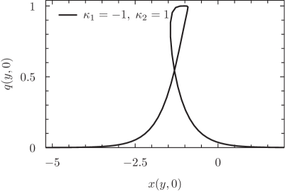
Figure 1: Parametric plots of $q(y,t)$ versus $x(y,t)$ at instant $t=0$. Similar behaviour is obtained for $r(y,t)$. The solutions keep their form unchanged during $t$ evolution.

6.5 From SPE to sine-Gordon

This section is a particular case of a more general result presented in the next section, but because the hodograph transformation $(y,s)\to(x,t)$ previously introduced [5, 7, 8] comes out so naturally from our definition (6.33), we will consider it first and it will also serve as a motivation for the forthcoming section. The model (4.25) is obtained from (4.22) when $v=u$, or equivalently $r=q$, thus imposing this restriction upon (6.34) we get

$$\chi=-\dfrac{\psi e^{-2\phi}}{1+\psi^{2}},$$ (6.37)

which substituted in the first relation of (6.11) yields

$$e^{-2\phi}=1+\psi^{2},\qquad\chi=-\psi.$$ (6.38)

Therefore, (6.33), note also (6.30), can be written in terms of one of the fields only

$$\alpha=\gamma^{-1}=\dfrac{1-\psi^{2}}{1+\psi^{2}}=\dfrac{1-\chi^{2}}{1+\chi^{2}}=2e^{2\phi}-1.$$ (6.39)

Reminding from the trigonometric identity $\cos\theta=2\cos^{2}\tfrac{\theta}{2}-1$, the relation (6.39) strongly suggests the parametrization

$$\alpha=\gamma^{-1}=\cos\theta,\qquad e^{\phi}=\cos\dfrac{\theta}{2},\qquad\psi=-\chi=\tan\dfrac{\theta}{2}.$$ (6.40)

The transformation (6.28) implies $u_{x}=\alpha^{-1}u_{y}$, but $q=u_{x}$ so from (6.34) we therefore have

$$u_{y}=-2\chi e^{2\phi}=2\tan\tfrac{\theta}{2}\cos^{2}\tfrac{\theta}{2}=\sin\theta.$$ (6.41)

Squaring $u_{x}=\alpha^{-1}u_{y}$ we have

$$u_{x}^{2}=(\cos^{2}\theta)^{-1}\left(1-\cos^{2}\theta\right)=\dfrac{1}{\alpha^{2}}-1,\qquad\gamma^{2}=1+u_{x}^{2},$$ (6.42)

which is the relation from where [8] started. Deriving both sides of (6.42) and plugging into the equations of motion (4.22) (with $v=u$) we have the conservation law (6.27) and its reciprocal (6.26), namely

$$\partial_{t}\gamma=\partial_{x}\left(2u^{2}\gamma\right),\qquad\partial_{s}\alpha=\partial_{y}\left(-2u^{2}\right).$$ (6.43)

Using (6.40) and (6.41) in the second equation of (6.43), we finally get the sine-Gordon model

$$u=\tfrac{1}{4}\theta_{s},\qquad\theta_{ys}=4\sin\theta.$$ (6.44)

6.6 From 2-SPE to Lund-Regge

Let us remind from the identities $q=u_{x}$, $r=v_{x}$, $\alpha=\tfrac{1}{\gamma}$ and $\partial_{x}=\alpha^{-1}\partial_{y}$. Taking the product of both terms in (6.34) yields

$$\gamma^{2} =1+u_{x}v_{x},$$ (6.45a)

$$\alpha^{2} =1-u_{y}v_{y}.$$ (6.45b)

Deriving (6.45a) and replacing into (4.22a) one gets

$$2\dfrac{\gamma\gamma_{t}}{v_{x}}=\dfrac{u_{x}v_{xt}}{v_{x}}+4u+4\dfrac{uv\gamma\gamma_{x}}{v_{x}}-2\dfrac{uvu_{x}v_{xx}}{v_{x}}+2u_{x}^{2}v+2u\left(\gamma^{2}-1\right),$$ (6.46)

while from (4.22b) one has

$$\dfrac{u_{x}v_{xt}}{v_{x}}=4\dfrac{u_{x}v}{v_{x}}+2\dfrac{uvu_{x}v_{xx}}{v_{x}}+2u_{x}^{2}v+2u\left(\gamma^{2}-1\right).$$ (6.47)

Simplifying these two last equations we obtain the respective conservation law (6.26) and its reciprocal (6.27), which read

$$\partial_{t}\gamma =\partial_{x}\left(2uv\gamma\right),$$ (6.48a)

$$\partial_{s}\alpha =\partial_{y}\left(-2uv\right).$$ (6.48b)

Deriving (6.45b) with respect to $s$ and using (6.48b) we therefore have

$$v_{y}\left(u_{ys}-4\alpha u\right)+u_{y}\left(v_{ys}-4\alpha v\right)=0.$$ (6.49)

A consistency condition, e.g. under the choice $v=u$, requires that

$$u_{ys} =4\alpha u,$$ (6.50a)

$$v_{ys} =4\alpha v.$$ (6.50b)

From (6.50) we have $u$ and $v$ in terms of $\chi,\phi,\psi$, once $u_{y}=\alpha q$ and $v_{y}=\alpha r$ are given from (6.34). However, for our purposes, it is more convenient to introduce the auxiliary fields

$$\bar{\psi}\equiv\psi e^{\phi},\qquad\bar{\chi}\equiv\chi e^{\phi}.$$ (6.51)

Then, the relations (6.11) read

$$\partial_{y}\phi=\dfrac{\bar{\chi}\partial_{y}\bar{\psi}}{1+\bar{\chi}\bar{\psi}},\qquad\partial_{s}\phi=\dfrac{\bar{\psi}\partial_{s}\bar{\chi}}{1+\bar{\chi}\bar{\psi}},$$ (6.52)

and (6.34) yields

$$u_{y} =2\bar{\psi}\left(1+\bar{\chi}\bar{\psi}\right)e^{-\phi},$$ (6.53a)

$$v_{y} =-2\bar{\chi}e^{\phi}.$$ (6.53b)

Replacing (6.53) into (6.50) we obtain

$$u =\dfrac{\partial_{s}\bar{\psi}e^{-\phi}}{2},$$ (6.54a)

$$v =-\dfrac{\partial_{s}\bar{\chi}e^{\phi}}{2\left(1+\bar{\chi}\bar{\psi}\right)},$$ (6.54b)

and if we employ (6.51) with (6.15), the solution in terms of tau functions reads

$$u(y,s) =\dfrac{\tau_{00}\partial_{s}\tau_{12}-\tau_{12}\partial_{s}\tau_{00}}{2\tau_{00}\tau_{11}},$$ (6.55a)

$$v(y,s) =-\dfrac{\tau_{11}}{2\tau_{00}}\dfrac{\tau_{00}\partial_{s}\tau_{21}-\tau_{21}\partial_{s}\tau_{00}}{\tau_{00}^{2}+\tau_{12}\tau_{21}}.$$ (6.55b)

Deriving (6.54) with respect to $y$ and equating to (6.53), after using (6.52), we obtain the Lund-Regge model [26, 27]

$$\bar{\psi}_{ys}-\dfrac{\bar{\chi}\bar{\psi}_{y}\bar{\psi}_{s}}{1+\bar{\chi}\bar{\psi}}-4\bar{\psi}\left(1+\bar{\chi}\bar{\psi}\right) =0,$$ (6.56a)

$$\bar{\chi}_{ys}-\dfrac{\bar{\psi}\bar{\chi}_{y}\bar{\chi}_{s}}{1+\bar{\chi}\bar{\psi}}-4\bar{\chi}\left(1+\bar{\chi}\bar{\psi}\right) =0.$$ (6.56b)

Therefore, we have explicitly established an equivalence between the 2-SPE (4.22) and the Lund-Regge model (6.56).

As a particular case, choosing $\bar{\chi}=-\bar{\psi}$ we have

$$\bar{\psi}_{ys}+\dfrac{\bar{\psi}\bar{\psi}_{y}\bar{\psi}_{s}}{1-\bar{\psi}^{2}}-4\bar{\psi}\left(1-\bar{\psi}^{2}\right)=0,$$ (6.57)

which is the sine-Gordon equation (6.44) through the parametrization $\bar{\psi}=\sin\tfrac{\theta}{2}$.

7 Conclusions

We have proposed a higher grading construction for integrable hierarchies. When the algebra ${\widehat{\mathcal{G}}}=\hat{A}_{1}$ with homogeneous gradation is chosen, this construction yields the WKI hierarchy. The previous known models [6] constitute the positive flows. We have extended the WKI hierarchy to negative flows, where the first negative flow yields the two-component field generalization of the short pulse equation [4]. Therefore, it is clear that in all these models underlie the same algebraic structure. Some novel integrable nonautonomous models were also proposed, mixing a positive with a negative flow. These integrable mixed models may have applications in nonlinear optics, specially concerning accelerated ultra-short optical pulses [22].

We have derived local and nonlocal charges from the Riccati form of the spectral problem. The nonlocal charges are usually more difficult to be obtained, and we have shown how they can be constructed through positive power series expansion in the spectral parameter. This method can be used to other integrable hierarchies as well.

We have demonstrated that the dressing method is unable to solve the WKI hierarchy, which in fact, does not have the usual solitonic type of solution, travelling with constant velocity. Combining gauge and reciprocal Bäcklund transformations we have established the precise connection between the whole WKI and AKNS hierarchies, mapping each flow of both hierarchies. This gives a formal explanation of various relations scattered through the literature, for instance, the connection between the elastic beam and mKdV equations [28], the relation between the Dym and KdV equations [29] and also the recent hodograph transformation [5] relating the short pulse equation to the sine-Gordon model. We considered explicitly this mapping between the first negative flows of the WKI and AKNS hierarchies, and demonstrated the correspondence between the novel two-component short pulse equation (4.22) and the Lund-Regge model (6.56), generalizing the previous hodograph transformation (1.3). In the same way that the notorious Miura transformation relates the KdV and mKdV hierarchies, which in fact is a gauge transformation, the combination of gauge followed by a reciprocal transformation yields more involved relations. We believe that our results show this explicitly, and the same approach can be applied to other integrable hierarchies following our construction. This relations will generate exotic solitonic solutions, like the loop-solitons, arising from an implicit space-time dependence.

We have constructed solutions for the whole WKI hierarchy, writing them in terms of the known AKNS tau functions. We have motivated that the models within the positive flows of the WKI hierarchy describe larger amplitude solutions than the corresponding usual solitonic solutions, which is expected from the higher nonlinearity contained in the equations of motion. We believe that these models may have particular interesting applications that were not further explored.

Finally, we stress that our higher grading construction is general and other affine Lie algebras can be considered, which will give rise to novel integrable models. For instance, a $n$-component generalization can be considered with the algebra $\hat{A}_{n-1}\sim\hat{s\ell}_{n}$. The technique of using gauge plus reciprocal transformations will be well suited to deal with these cases.

Acknowledgments

We thank CAPES, CNPQ and Fapesp for financial support.

References

- [1] H. Aratyn, J. F. Gomes, and A. H. Zimerman, Algebraic construction of integrable and super integrable hierarchies, in Proc. of the XI-th International Conference Symmetry Methods in Physics, (Prague, Czech Republic), June, 2004. hep-th/0408231.
- [2] H. Aratyn, J. Gomes, E. Nissimov, S. Pacheva, and A. Zimerman, Symmetry flows, conservation laws and dressing approach to the integrable models, in Integrable Hierarchies and Modern Physical Theories (H. Aratyn and A. S. Sorin, eds.), vol. 18 of Nato Science Serries II, (Chicago, USA), pp. 243–275, Kluwer, July, 2000. nlin/0012042.
- [3] O. Babelon and D. Bernard, Affine solitons: a relation between tau functions, dressing and Bäcklund transformations, Int. J. Mod. Phys. A8 (1993), no. 3 507–543, [hep-th/9206002].
- [4] T. Schäfer and C. Wayne, Propagation of ultra-short optical pulses in cubic nonlinear media, Physica D196 (2004), no. 1–2 90–105.
- [5] A. Sakovich and S. Sakovich, The short pulse equation is integrable, J. of Phys. Soc. of Japan 74 (2005), no. 1 239–241, [nlin/0409034].
- [6] M. Wadati, K. Konno, and Y. H. Ichikawa, New integrable nonlinear evolution equations, J. of Phys. Soc. of Japan 47 (1979), no. 5 1698–1700.
- [7] A. Sakovich and S. Sakovich, Solitary wave solutions of the short pulse equation, J. of Phys. A: Math. Gen. 39 (2006), no. 22 L361, [nlin/0601019].
- [8] Y. Matsuno, Periodic solutions of the short pulse model equation, J. Math. Phys. 49 (2008), no. 7 073508, [arXiv:0912.2576].
- [9] J. C. Brunelli, The short pulse hierarchy, J. Math. Phys. 46 (2005), no. 12 123507, [nlin/0601015].
- [10] Y. H. Ichikawa, K. Konno, and M. Wadati, Nonlinear transverse oscillation of elastic beams under tension, J. of Phys. Soc. of Japan 50 (1981), no. 5 1799–1802.
- [11] J. Brunelli, The bi-Hamiltonian structure of the short pulse equation, Phys. Lett. A353 (2006), no. 6 475–478, [nlin/0601014].
- [12] Y. Matsuno, A novel multi-component generalization of the short pulse equation and its multisoliton solutions, J. Math. Phys. 52 (2011), no. 12 123702, [arXiv:1111.1792].
- [13] J.-L. Gervais and M. V. Saveliev, Higher grading generalizations of the Toda systems, Nucl. Phys. B453 (1995) 449–476, [hep-th/9505047].
- [14] L. A. Ferreira, J.-L. Gervais, J. Sanchez Guillen, and M. Saveliev, Affine Toda systems coupled to matter fields, Nucl. Phys. B470 (1996) 236–290, [hep-th/9512105].
- [15] P. Assis and L. Ferreira, The Bullough-Dodd model coupled to matter fields, Nucl. Phys. B800 (2008) 409–449, [arXiv:0708.1342].
- [16] J. F. Gomes, G. R. de Melo, and A. H. Zimerman, A class of mixed integrable models, J. of Phys. A: Math. Theor. 42 (2009), no. 27 275208, [arXiv:0903.0579].
- [17] M. Wadati, H. Sanuki, and K. Konno, Relationships among inverse method, Bäcklund transformation and an infinite number of conservation laws, Prog. Theor. Phys. 53 (Feb., 1975) 419–436.
- [18] Y. Ishimori, A relationship between the Ablowitz-Kaup-Newell-Segur and Wadati-Konno-Ichikawa schemes of the inverse scattering method, J. of Phys. Soc. of Japan 51 (1982), no. 9 3036–3041.
- [19] C. Rogers and P. Wong, On reciprocal Bäcklund transformations of inverse scattering schemes, Phys. Scripta. 30 (1984), no. 1 10.
- [20] T. Shimizu and M. Wadati, A new integrable nonlinear evolution equation, Prog. Theor. Phys. 63 (1980), no. 3 808–820.
- [21] J. C. Brunelli and S. Sakovich, “On integrability of the Yao-Zeng two-component short-pulse equation.” 2012.
- [22] H. Leblond and D. Mihalache, Few-optical-cycle solitons: Modified Korteweg-de Vries sine-Gordon equation versus other nonlinear slowly-varying-envelope-approximation models, Phys. Rev. A79 (Jun, 2009) 063835.
- [23] H. Aratyn, L. A. Ferreira, J. F. Gomes, and A. H. Zimerman, The complex sine-Gordon equation as a symmetry flow of the AKNS hierarchy, J. of Phys. A: Math. Gen. 33 (2000), no. 35 L331, [nlin/0007002].
- [24] I. Cabrera-Carnero, J. Gomes, G. Sotkov, and A. H. Zimerman, Vertex operators and soliton solutions of affine Toda model with symmetry, J. of Phys. A: Math. Gen. 37 (June, 2004) 6375–6389, [hep-th/0403042].
- [25] J. Gomes, G. França, and A. Zimerman, Dressing approach to the nonvanishing boundary value problem for the AKNS hierarchy, J. of Phys. Conf. Ser. 343 (Feb., 2012) 012039, [arXiv:1111.5372].
- [26] F. Lund and T. Regge, Unified approach to strings and vortices with soliton solutions, Phys. Rev. D14 (Sep, 1976) 1524–1535.
- [27] F. Lund, Classically solvable field theory model, Ann. of Phys. 115 (1978), no. 2 251–268.
- [28] Y. Ishimori, On the modified Korteweg-de Vries soliton and the loop soliton, J. of Phys. Soc. of Japan 50 (Aug., 1981) 2471.
- [29] W. Hereman, P. P. Banerjee, and M. R. Chatterjee, Derivation and implicit solution of the Harry Dym equation and its connections with the Korteweg-de Vries equation, J. of Phys. A: Math. Gen. 22 (1989), no. 3 241.