Thermally driven classical Heisenberg model in one dimension

Abstract

We study thermal transport in a classical one-dimensional Heisenberg model employing a discrete time odd even precessional update scheme. This dynamics equilibrates a spin chain for any arbitrary temperature and finite value of the integration time step $\Delta t$. We rigorously show that in presence of driving the system attains local thermal equilibrium which is a strict requirement of Fourier law. In the thermodynamic limit heat current for such a system obeys Fourier law for all temperatures, as has been recently shown [A. V. Savin, G. P. Tsironis, and X. Zotos, Phys. Rev. B 72, 140402(R) (2005)]. Finite systems, however, show an apparent ballistic transport which crosses over to a diffusive one as the system size is increased. We provide exact results for current and energy profiles in zero- and infinite-temperature limits.

I Introduction

The flow of heat from a hot source to a cold sink is conventionally described in the hydrodynamic limit by Fourier law $J=-\kappa\,\nabla T$, where $J$ is the steady state thermal current set up in response to the temperature gradient $\nabla T$ and $\kappa$ is the (finite) thermal conductivity. There have been several attempts Lebo ; Lepri at a microscopic ‘derivation’ of this phenomenological equation which, however, could not be achieved yet. Needless to say, in spite of the huge amount of studies over decades, our understanding of this basic transport phenomenon is still not quite satisfactory. It has been found that in a variety of one-dimensional models Lebo ; Lepri ; AD-rev the thermal current scales with system size as $L^{-\alpha}$ where $\alpha\leq 1$. This corresponds to a diverging heat conductivity in the thermodynamic limit and thus is a violation of Fourier law. It is quite a surprise that Fourier law, which has been remarkably consistent with experimental results in general, is found to be invalid in many models in low dimension. For three-dimensional systems Fourier law is believed to be generically true but a rigorous proof is still lacking AD-rev .

In a recent work it has been shown numerically (using the Green Kubo approach Kubo ) that a classical one-dimensional Heisenberg spin model obeys Fourier law at all temperatures savin05 . Also, it has been known for quite some time now that at infinite temperature such spin systems follow the energy diffusion phenomenology in the hydrodynamic limit landau . On the other hand, the 1D spin-$\frac{1}{2}$ quantum Heisenberg model (QHM) being integrable, violates Fourier law and thermal transport is ballistic integr ; hlubek . For recent reviews on the theoretical and experimental developments in quantum spin models see QM and references therein. One of the basic assumptions for the validity of Fourier law lies in the establishment of local thermal equilibrium (LTE) in the system Lebo ; LTE ; Lepri , which allows one to define thermodynamic quantities in the steady state such as pressure, temperature etc., locally. Most studies, however, focus on the issue of whether Fourier law is obeyed or not, without explicitly verifying the existence of LTE. In fact, it is known that a system may settle down to a nonequilibrium steady state (NESS) which does not satisfy the essential requirement of having LTE e.g., XY model, Lorentz gas model AD-DD-XY . It is believed that the absence of LTE in these examples is due to the existence of infinitely many local conserved quantities in the dynamics AD-DD-XY . Many of the theoretical approaches AD-rev ; Lepri rely on Linear response theory (Green-Kubo formula) where conductivity is measured by computing two point current-current time correlation which assumes quasi-equilibrium. The Kubo formula Kubo is strictly valid close to equilibrium and in the limit $L\to\infty$, and so considerable care should be taken in making conclusions from experimental or simulation data which deal with finite system size and drive AD-rev .

In this paper, we study thermal transport properties of a classical one-dimensional Heisenberg spin model. We use a discrete time odd even (DTOE) dynamics which, unlike standard numerical integration schemes, evolves the system to the correct steady state without violating the required conservations. We explicitly show that the DTOE dynamics equilibrates a closed system and the final state is the same for all nonzero values of $\Delta t$. With two equal temperature baths attached to its two ends, the system eventually equilibrates under the DTOE dynamics and attains the temperature of the baths. When temperature of the heat baths is different, thermal equilibrium is established in the system locally. With finite drive, we study in details the transport properties of the system e.g., thermal current $J$, energy profiles, conductivity $\kappa$ without invoking linear response theory. We find that, in the thermodynamic limit, the system obeys Fourier law at all temperatures which is consistent with the recent study savin05 . For a finite system however, there is a characteristic temperature below which the system crosses over to a regime where transport becomes ballistic. We present exact results for thermal current and energy profile in the limit $T\to 0$ and $T\to\infty$.

The paper is organized as follows. In Sec. II and Sec. II.1 we describe the model and the spin dynamics in detail. We then look into the equilibration of a closed spin chain under this dynamics in Sec. III. In Sec. IV we study, analytically and numerically, the transport properties of the model in presence of thermal baths. We present a discussion and summarize our main results in Sec. V.

II Model

Consider classical Heisenberg spins $\{\vec{S_{i}}\}$ (three-dimensional unit vectors) on a one-dimensional regular lattice of length $L$ $(1\leq i\leq L)$ with periodic boundary conditions. The microscopic Hamiltonian is given by

$$\mathcal{H}=-K\sum_{i=1}^{L}\vec{S}_{i}\cdot\vec{S}_{i+1}=-K\sum_{i=1}^{L}\cos\theta_{i},$$ (1)

where the spin-spin interaction is ferromagnetic for coupling $K>0$ and anti-ferromagnetic for $K<0$. For all the numerical results shown in the paper $K$ has been set to unity. Here $\theta_{i}$ is the relative angle between $\vec{S}_{i}$ and $\vec{S}_{i+1}.$ The microscopic equation of motion can be taken as

$$\frac{d}{dt}{\vec{S}_{i}}=\vec{S}_{i}\times\vec{B}_{i},$$ (2)

where $\vec{B}_{i}=K(\vec{S}_{i-1}+\vec{S}_{i+1})$ is the local molecular field experienced by the spin at site $i$. Clearly, Eq. (2) conserves (i) the magnitude of the individual spin vectors $S_{i}^{2}$ and (ii) the energy density

$${E}=\frac{1}{L}\sum_{i=1}^{L}\epsilon_{i},~{}~{}~{}{\rm where}~{}~{}\epsilon_{i}=-K\vec{S}_{i}\cdot\vec{S}_{i+1}.$$ (3)

Note that this dynamics is the classical equivalent of the quantum dynamics for a spin-$\frac{1}{2}$ QHM. Just as the commutation relations of quantum spin operators, the classical spins components obey the standard Poisson bracket relations for angular momentum.

However, there is a fundamental difference between the quantum spin-$\frac{1}{2}$ model and the classical model. The spin-$\frac{1}{2}$ QHM is integrable, whereas all higher spin $(S\geq 1)$ QHMs (and therefore the classical model which corresponds to $S\to\infty$) are non-integrable. Consequently, there are infinitely many conserved quantities in a spin-$\frac{1}{2}$ QHM (which includes the energy current) and the thermal transport is ballistic integr . On the other hand, only the total spin and the total energy are conserved in the corresponding classical model, and thus one expects transport properties to be normal.

Since we wish to study thermal transport, typically far away from equilibrium (for which no general theoretical formulation is known), we need to integrate Eq. (2) numerically keeping the conservations intact. In the next section, we show that a straightforward numerical integration of Eq. (2) fails to conserve either $S_{i}^{2}$ or $E$ or both. We also discuss in detail the advantages of using the discrete time odd even dynamics (DTOE).

II.1 Why DTOE dynamics?

To integrate the equation of motion numerically one would naively start off with a finite difference equation of the form

$$\vec{S}_{i,t+1}=\vec{S}_{i,t}+\Delta t\,\,\left[\vec{S}\times\vec{B}\right]_{i,t}$$ (4)

and update all the spins at time $t$ to obtain their values at $t+1$. Such an Eulerian scheme cannot be used for this system because of the fact that it does not satisfy the required $S_{i}^{2}$ and $E$ conservations. It is easy to calculate the energy $E(t)$ and $S_{i}^{2}(t)$ in the Euler scheme using Eq. (4) which comes out to be

$$E(t) = E(0)-K(\Delta t)^{2}\sum_{\tau=0}^{t-1}\sum_{i=1}^{L}\left[\vec{S}\times\vec{B}\right]_{i,\tau}\cdot\left[\vec{S}\times\vec{B}\right]_{i+1,\tau}$$

$${S}^{2}_{i}(t) = S^{2}_{i}(0)+(\Delta t)^{2}\sum_{\tau=0}^{t-1}\left[\vec{S}\times\vec{B}\right]^{2}_{i,\tau}$$

Thus, any finite $\Delta t$, however small, breaks both the conservations and consequently the scheme fails for all practical purposes [see Fig. 1(a)]. A way to keep the magnitude of the spin vectors conserved is to use a spin precession dynamics

$$\vec{S}_{i,t+1}=\left[\vec{S}\cos\phi+(\vec{S}\times\hat{B})\sin\phi+(\vec{S}\cdotp\hat{B})\hat{B}(1-\cos\phi)\right]_{i,t},$$ (6)

where $\hat{B}_{i}=\vec{B}_{i}/|\vec{B}_{i}|$ and $\phi_{i}=|\vec{B}_{i}|\Delta t$ goldstein , instead of Eq. (4). A spin $\vec{S}_{i}$, when updated using Eq. (6), undergoes a precessional motion about the instantaneous local molecular field $\vec{B_{i}}$ which keeps its magnitude unaltered i.e., $S_{i,t+1}^{2}=S_{i,t}^{2}$. However, this precessional dynamics does not preserve energy conservation. Expanding Eq. (6) in powers of $\Delta t$ and retaining terms up to $\mathcal{O}(\Delta t)$ one obtains back the first equation of Eq. (LABEL:delta_E) and thus energy conservation still remains violated for any $\Delta t>0$. This has also been shown numerically in Fig. 1(b). Other numerical schemes such as Runge-Kutta, predictor corrector method etc., will also fail to preserve the energy conservation for the same reason.

We now describe an odd-even update rule which along with the precessional dynamics has been herein referred to as the DTOE dynamics. Starting from a spin configuration $\{\vec{S}_{i}\}$, we numerically implement the dynamics described in Eq. (1) by alternate parallel updates of the spins on odd and even sublattices. Henceforth, we refer to these two groups of spins as odd and even spins. At each Monte Carlo step (MCS), first only even spins are updated using the spin precession dynamics Eq. (6) and the odd spins are kept unaltered. Next, the spins on the odd sublattice are updated similarly. These two steps update all the spins $\{\vec{S}_{i}\}$ in the system and constitute one MCS. It is straightforward to check that update of any spin $\vec{S}_{i}$ affects only the energy of the neighboring bonds $\epsilon_{i-1}$ and $\epsilon_{i}$ but their sum ($\epsilon_{i-1}+\epsilon_{i}$) remains constant. Thus DTOE dynamics is strictly energy conserving.

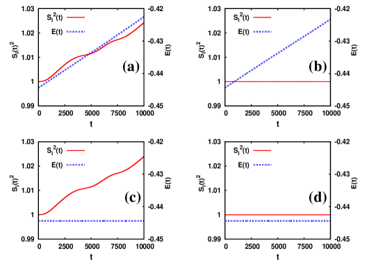
Figure 1: (Color online) Evolution of spin magnitude $S_{i}^{2}$ and the energy density $E$. (a) Parallel update using Eq. (4) (b) Parallel update using Eq. (6) (c) Odd even update using Eq. (4) (d) DTOE. For all the figures $\Delta t=0.001$ and $L=10000$. Thus, only DTOE dynamics conserves both $E$ and $S_{i}^{2}$.

Clearly, the spin precession dynamics conserves the magnitude of the spin vectors while, energy conservation is maintained by the odd-even update rule (see Fig. 1). A recent paper DTOE has also employed this odd-even precessional dynamics with large $\Delta t$ to study transport in a classical Heisenberg model (1D periodic spin system) in presence of quenched disorder numerically. Although this dynamics does not directly follow from the equation of motion [Eq. (2)], it can be used to study the system numerically provided that the system equilibrates for any arbitrary $\Delta t$. In the next section, we study the equilibration of a closed system when evolved using DTOE dynamics.

III Closed system

We first investigate whether a closed system (i.e., with periodic boundary conditions) under DTOE dynamics evolves to the correct steady state for different values of $\Delta t$. To do this, first we compute the correlation functions of the system in canonical ensemble, subjected to temperature $T$ and then show numerically that the same correlation functions are obtained from a closed system with a fixed energy (i.e. in a micro-canonical ensemble).

The partition function of the system Joyce with the Hamiltonian given by Eq. (2) is

$$\mathcal{Z}=\int\prod_{i=1}^{L}\left(\frac{d\vec{S}_{i}}{4\pi}\right)\exp(\beta K\sum_{i=1}^{L}\vec{S}_{i}\cdot\vec{S}_{i+1}),$$ (7)

$\beta=1/k_{B}T$ and $k_{B}$ has been set equal to unity henceforth. The two-spin correlation functions are therefore given by

$$C_{lr}=\langle P_{l}(\vec{S}_{i}\cdotp\vec{S}_{i+r})\rangle=\left[\frac{\lambda_{l}(\beta K)}{\lambda_{0}(\beta K)}\right]^{r},$$ (8)

where $P_{l}$ are Legendre polynomials and

$$\lambda_{l}(k)=\frac{1}{2}\int_{-1}^{1}P_{l}(x)e^{kx}dx.$$ (9)

These correlation functions can be written explicitly in terms of the Langevin function ${\mathcal{L}}(x)$, for example,

$$C_{1r}=\left[{\mathcal{L}}(\beta K)\right]^{r}\;\;\;\;\;\;\;\;\;C_{2r}=\left[1-3\mathcal{L}(\beta K)/(\beta K)\right]^{r}.$$ (10)

It is evident that average energy of the system is $-KC_{11}$ and thus, a closed system with a fixed energy density $E$ has an effective $\beta={\mathcal{L}}^{-1}(-E/K)/K$.

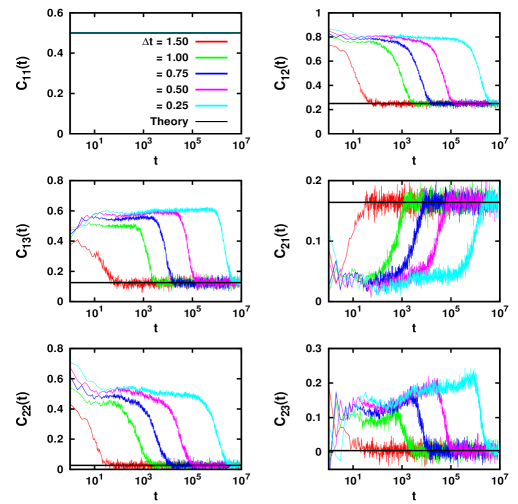
Figure 2: (Color online) Semi-log plots for the evolution of equal-time correlations $C_{11}$, $C_{12}$, $C_{13}$, $C_{21}$, $C_{22}$, $C_{23}$ as obtained from simulation for a closed system of $L=1000$. DTOE dynamics has been used with time-step $\Delta t=1.5,1.0,0.75,0.5,0.25$ and $E=-0.5$.

First, let us compute the equal-time spin-spin correlations $C_{lr}(t)$ for a closed system and check that these evolve to the stationary value given by Eq. (10). The time series for $C_{1r}(t)$ and $C_{2r}(t)$ with different $r$ values are shown in the Fig. 2. We find that the correlation functions for different $\Delta t$ saturate to the same value at late times. In Fig. 3 the time averaged equilibrium correlation functions $C_{lr}$ obtained from systems set at different energies, are also found to be in remarkable agreement with Eq. (10). Thus the DTOE dynamics equilibrates the system irrespective of the value of $\Delta t$; $\Delta t$ only alters the equilibration time of the system. A larger $\Delta t$ is preferable as equilibration in this case is attained faster.

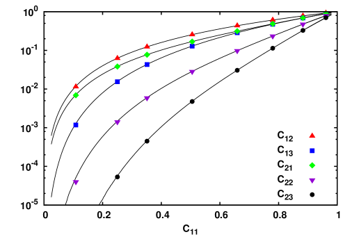
Figure 3: (Color online) Semi-log plot for different equilibrium correlations $C_{lr}$ for $l=1,2$ vs. $C_{11}=-E$ obtained from simulation (points) and compared with theory (lines) for a periodic lattice of $L=1000$. DTOE dynamics has been used with time-step $\Delta t$ = 1.0.

IV Open system

IV.1 Modeling heat bath

In order to study energy transport in the system, we now look into an open system with heat baths attached to its two ends. The left and right baths are set at temperatures $1/\beta_{l}$ and $1/\beta_{r}$ respectively. Each bath is known as a stochastic thermal bath bath which means that it is in equilibrium at its respective temperature and has a Boltzmann energy distribution. The baths are implemented by introducing two additional sites $i=0$ and $i=L+1$ in the system with spins $\vec{S}_{0}$ and $\vec{S}_{L+1}$ respectively. These pairs of spins ($\vec{S}_{0},\vec{S}_{1}$) and ($\vec{S}_{L},\vec{S}_{L+1}$) behave as stochastic heat baths at two ends of the system. The baths are in equilibrium at their respective temperatures and the bond energies $\epsilon_{0}$ and $\epsilon_{L}$ have a Boltzmann distribution

$$P(\epsilon_{0})\sim e^{-\beta_{l}\epsilon_{0}}~{}{\rm and}~{}P(\epsilon_{L})\sim e^{-\beta_{r}\epsilon_{{}_{L}}}.$$ (11)

The interaction strength of the bath spins with the system is taken to be $K$, and therefore both $\epsilon_{0}$ and $\epsilon_{L}$ are bounded in the range $(-K,K)$. Thus the mean energies of the left and the right bath are given by

$$E_{l}=\langle\epsilon_{0}\rangle=-K\mathcal{L}(\beta_{l}K)~{}{\rm and}~{}E_{r}=\langle\epsilon_{{}_{L}}\rangle=-K\mathcal{L}(\beta_{r}K).$$

Following the odd-even rule, the spin $\vec{S}_{0}$ is updated along with the even spins, whereas $\vec{S}_{L+1}$ is updated with odd (even) spins depending on whether $L$ is even (odd). To update $\vec{S}_{0}$, first the energy of the bond $\epsilon_{0}$ between the spins $(\vec{S}_{0},\vec{S}_{1})$ is set to a value drawn randomly from $P(\epsilon_{0})$ given in Eq. (11). The spin $\vec{S}_{0}$ is then constructed such that $\epsilon_{0}=-K\vec{S}_{0}\cdotp\vec{S}_{1}.$ During this update $\vec{S}_{1}$ is not modified as it belongs to the odd sublattice. At the right end, the spin $\vec{S}_{L+1}$ is updated similarly. We must mention that energy conservation is violated during update of bath spins. The interaction of the bath spins with the neighboring spins allow boundary fluctuations to propagate into the bulk, thus inducing a thermal current in the system.

Although the closed system equilibrates under DTOE dynamics, it is not guaranteed that an open system will also equilibrate when baths are attached to its two ends. Before studying the system with a finite drive, we study the equilibration of an open system with baths maintained at the same temperature, thus still keeping the system in equilibrium at temperature $T$, i.e. $\beta_{l}=\beta=\beta_{r}.$ With baths maintained at equal temperature $T$, the spin chain is expected to eventually reach a thermodynamic equilibrium corresponding to the bath temperature $T$. We have calculated numerically the average energy of the system $\langle E\rangle$ for different values of $\beta=10,1,$ and $0.1$, which is shown in Fig. 4(a). Evidently, at late times $\langle E\rangle$ approaches the stationary value $-K{\cal L}(K\beta)$. Figure 4(b) shows that the system attains a unique stationary state consistent with the bath temperature and this final state is independent of the value of $\Delta t$ used. Similar to the case of the closed system, $\Delta t$ decides only the equilibration time of the system. We also measure the equilibrium correlations $C_{lr}$ which are shown in Fig. 4(c) where the numerical values are found to be in agreement with Eq. (10). This assures us that for any nonzero $\Delta t$ the DTOE dynamics is no different from the equation of motion (2), and allows the system to attain the correct equilibrium state.

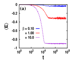
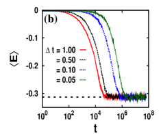
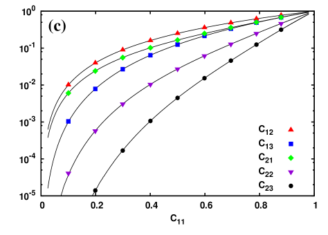
Figure 4: (Color online) Semi-log plot for the evolution of average energy $\langle E\rangle$ for a system with $\beta_{l}=\beta_{r}=\beta$ for (a) $\beta=0.1,1.0,10.0$ and a fixed $\Delta t=1.0$ and (b) $\Delta t=1.0,0.5,0.1,0.05$ and a fixed $\beta=1.0.$ (c) Different correlations $C_{lr}$ obtained from simulation (points) are shown as a function of $C_{11}$ along with the functions Eq. (10) (lines); $L=1000$ and $\Delta t=1.0.$

IV.2 LTE in a driven system

A finite thermal drive is imposed on the spin chain by setting the two heat baths at unequal temperature, i.e. $\beta_{l}\neq\beta_{r}$. The bath and bulk spins are updated as mentioned in the previous section. Now, since the bath temperatures are unequal, the system is driven out of equilibrium. However, it may still be possible to define a temperature like thermodynamic variable locally in a region if the average energy of the sites $\langle\epsilon_{i}\rangle$ belonging to that region is not too different from each other. The system is said to have local thermal equilibrium (LTE) if all the correlation functions measured in this local region are identical to those of a thermodynamically large equilibrium system with an average energy $\langle\epsilon_{i}\rangle$.

Numerically, one measures the correlation functions $C_{lr}(x)$ locally over $n\ll L$ consecutive sites about $x=i/L$ such that the average energy of these $n$ sites is almost equal to each other. For a system of size $L=1000$ we measure $C_{lr}(x)$ up to three nearest neighbors for $l=1,2$ and by averaging them over $n=20$ sites. This is shown in Fig. 5, where we have shown $C_{lr}(x)$ for different $x$ (in the range $(0,1)$) as a parametric function of $C_{11}(x)$. For comparison, the equilibrium curves (from Eq. (10)) are also shown in the figure as solid lines. An excellent match with the equilibrium functions assures that the driven spin system attains thermal equilibrium locally. Thus, following the equilibrium definition, we may define uniquely the local inverse temperature

$$\beta(x)\equiv\frac{1}{K}{\cal L}^{-1}(C_{11}(x)).$$ (12)

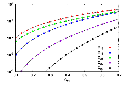
Figure 5: (Color online) Semi-log plot for different correlations $C_{lr}(x)$, where $0<x=i/L<1$, for $l=1,2$ vs. $C_{11}(x)$ obtained from simulation (points) and compared with Eq. (10) (lines) for a open system of $L=1000$. The average bath energies are $E_{l}=-0.7$ and $E_{r}=-0.1$. DTOE dynamics has been used with time-step $\Delta t=5.0$.

IV.3 Analytical Results

In the previous section we have seen that the driven system attains local thermal equilibrium, and thus a local temperature can be uniquely defined through Eq. (12). Therefore, the usual definition of Fourier law $J\propto\nabla T$ can also be equivalently expressed as $J\propto\nabla E.$ The thermal current and the energy profile are measured as described in the following. Since the DTOE dynamics alternately updates only half of the spins (but all the bond energies simultaneously), the energy of the bonds $\epsilon^{o}_{i}$ measured immediately after the update of odd spins is different from $\epsilon^{e}_{i}$ measured after the update of even spins. Clearly, this difference $\epsilon^{e}_{i}-\epsilon^{o}_{i}$ is a measure of the energy flowing through the $i$-th bond in each MCS. Thus the thermal current in the steady state is given by

$$J=\langle\epsilon^{e}_{i}-\epsilon^{o}_{i}\rangle$$ (13)

and the average energy of $i$-th bond is $\epsilon_{i}=\frac{1}{2}\langle\epsilon^{e}_{i}+\epsilon^{o}_{i}\rangle$. In fact, this expression for the current, in the limit $\Delta t\to 0$, is consistent with that obtained from the continuity equation $\dot{\epsilon}_{i}(t)=J_{i-1}(t)-J_{i}(t)$ where $\epsilon_{i}(t)=-K\vec{S}_{i}\cdot\vec{S}_{i+1}$ is the local energy density. Straightforward calculation using the continuity equation gives the instantaneous current across $i$-th bond

$$J_{i}(t)=K~{}\vec{S}_{i}\cdot(\vec{S}_{i+1}\times\vec{S}_{i+2}).$$ (14)

Again, when the $i$-th site (say, even) gets updated, the energy of the $i$-th bond is $\epsilon_{i}^{e}=-K~{}\vec{S}_{i}(t+1)\cdot\vec{S}_{i+1}(t)$ and after the subsequent update of odd sites it becomes $\epsilon_{i}^{o}=-K~{}\vec{S}_{i}(t+1)\cdot\vec{S}_{i+1}(t+1)$. Thus using Eq. (6), the instantaneous current (time is measured in units of $\Delta t$) across the $i$-th bond in the limit $\Delta t\to 0,$ reduces to

$$J_{i}(t)=\epsilon^{e}_{i}-\epsilon^{o}_{i}=K~{}\vec{S}_{i}\cdot(\vec{S}_{i+1}\times\vec{S}_{i+2}),$$ (15)

which is same as Eq. (14).

In the following, we show that the model with DTOE dynamics can be solved exactly in both $T\to 0$ and $T\to\infty$ limits to obtain analytical expressions for the energy current and energy profile. We show that energy transport in any finite system is ballistic in the limit $T\to 0$, whereas diffusive transport is observed for $T\to\infty.$

Ballistic Limit ($T\to 0$): In this limit, the spins are nearly aligned (hence $\vec{S}_{i}\times\vec{B}_{i}\simeq 0$) and, therefore, precess by small angles. In DTOE dynamics, the angle of precession is $\phi_{i}=|\vec{B}_{i}|\Delta t$ and so for small $\Delta t$ it mimics the dynamics of the system at low temperature. This equivalence can be utilised to write the energy function Eq. (2) in this limit as

$$\mathcal{H}\simeq-K\sum(1-\frac{1}{2}\theta_{i}^{2}),$$ (16)

which is similar to the energy function of a harmonic system. Since the DTOE dynamics is energy conserving, update of a spin $\vec{S}_{i}$ assures that $\theta_{i-1}^{2}+\theta_{i}^{2}$ remains invariant. Again, since the low temperature stationary state dynamics is governed by spin waves i.e., spin configuration whose orientation varies slowly with distance along the axis of the chain, the spins are locally parallel and $\theta_{i-1}+\theta_{i}$ is invariant in the $\Delta t\to 0$ limit. Thus the only allowed dynamics for the angle variable is

$$\theta_{i-1,t}\to\theta_{i,t+\Delta t}~{}~{}~{}~{}~{}\theta_{i,t}\to\theta_{i-1,t+\Delta t}.$$ (17)

Consequently, the energy of the bonds that connect to the $i$-th spin, namely $\epsilon_{i-1}$ and $\epsilon_{i}$, are mutually exchanged in this limit. Starting from $t=0$, the bond energies $\epsilon_{2i+1}$ for the odd bonds ‘move’ to the right and the even bond energies $\epsilon_{2i}$ ‘move’ to the left ballistically (without any scattering).

In the steady state, the average bond energies after the update of odd spins are $\langle\epsilon_{2i}^{o}\rangle=E_{l}$ and $\langle\epsilon_{2i+1}^{o}\rangle=E_{r}$ whereas, the same after the update of even spins become $\langle\epsilon_{2i}^{e}\rangle=E_{r}$ and $\langle\epsilon_{2i+1}^{e}\rangle=E_{l}$. Thus current $J=E_{l}-E_{r}$ is independent of the system size $L$ and thermal transport is ballistic. In the steady state, the temperature is same at all bulk sites, which is given by

$$T_{bulk}=\frac{K}{\mathcal{L}^{-1}\left(-\frac{E_{l}+E_{r}}{2K}\right)}$$ (18)

Note that this ballistic behavior is a consequence of the fact that the limit $\Delta t\to 0$ is taken before the thermodynamic limit $L\to\infty$. When $\Delta t\simeq 0$, the spins precess slowly since the precision angle $\phi_{i}$ is proportional to $K\Delta t$. Thus the effective correlation length diverges as $\Delta t\to 0$ and energy in any finite system would be transferred to arbitrary distances without being scattered.

Also, unlike the equilibrium case, the correlation functions of the driven system depend on $\Delta t$ when $L$ is finite. In the following, we argue that when $\Delta t\to 0$ the correlation length $\xi$ actually diverges. Since the energy profile in this limit is flat, a small change $\Delta t\to\Delta t^{\prime}$ will not change the correlation functions substantially. In order to keep the correlation functions (which are functions $\beta K$) unaltered, the inverse temperature $\beta$ should scale as $\beta^{\prime}=\beta\Delta t/\Delta t^{\prime}$, so that $K^{\prime}\beta^{\prime}=K\beta.$ Again, since the correlation length $\xi=\frac{1}{|\ln{\cal L}(K\beta)|}$ (calculated from Eq. (10) taking $C_{1r}\equiv e^{-r/\xi}$) diverges linearly with $\beta$ in the limit $\beta\to\infty$, we have

$$\xi\sim(\Delta t)^{-1}.$$ (19)

This indicates that the steady state energy profile also depends on $\Delta t$, which will be discussed later in section IV E (see Fig. 10(a)). We must mention here that this $\Delta t$ dependence is only a numerical artifact in finite systems. In fact, $1/\Delta t$ has to be compared with the two other length scales of the problem, namely, the size of the system $L$ and $1/T$ (as the correlation length also diverges in $T\to 0$ limit) and thus, the effective correlation length will appear to be $1/\Delta t$ only when both $L$ and $1/T$ are much smaller. In other words, for the numerical integration of Eq. (2), one must choose the integration time step $\Delta t$ larger than both $1/L$ and $T$ to avoid dependence of the steady state on $\Delta t.$ Therefore, a thermodynamically large system in this problem corresponds to a system with $L\gg 1/T\gg 1/\Delta t.$ In this limit, the correlation length $\xi$ remains smaller than $L$ for all $T>0$; the steady state behaviour is independent of $\Delta t$ and one recovers diffusive thermal transport (see Fig. 11 and related discussions later).

Diffusive limit ($T\to\infty$): In the other limit $T\to\infty$, the spin orientation is random and thus the dynamics is equivalent to large $\Delta t$ limit, where the precession angle $\phi$ is large and effectively the spin precesses by a random angle. Updating the $i$-th spin then results in random re-sharing of the bond energies $\epsilon_{i-1}$ and $\epsilon_{i}$ obeying the local energy conservation imposed by the DTOE dynamics. Effectively,

$$\epsilon_{i-1,t+1}=r(\epsilon_{i-1}+\epsilon_{i})_{t} \epsilon_{i,t+1}=(1-r)(\epsilon_{i-1}+\epsilon_{i})_{t}$$

where, $r$ is a uniform random number in the range $(0,1)$. This dynamics is similar to the diffusive dynamics discussed by Kipnis et. al. kipnis except the fact that here we use the DTOE dynamics. In the steady state, the average energies at different sites satisfy the following equations. Update of odd sites ensures that for $j=0,1,\dots,L/2,$

$$\langle\epsilon_{2i}^{o}\rangle = \left(\langle\epsilon_{2i}^{e}\rangle+\langle\epsilon_{2i+1}^{e}\rangle\right)/2$$ (21)

$$\langle\epsilon_{2i+1}^{o}\rangle = \left(\langle\epsilon_{2i}^{e}\rangle+\langle\epsilon_{2i+1}^{e}\rangle\right)/2$$ (22)

Similarly update of odd sites gives

$$\langle\epsilon_{2i-1}^{e}\rangle = \left(\langle\epsilon_{2i-1}^{o}\rangle+\langle\epsilon_{2i}^{o}\rangle\right)/2$$ (23)

$$\langle\epsilon_{2i}^{e}\rangle = \left(\langle\epsilon_{2i-1}^{o}\rangle+\langle\epsilon_{2i}^{o}\rangle\right)/2,$$ (24)

for $j=1,2,\dots,L/2$, along with the boundary conditions

$$\langle\epsilon_{0}^{e}\rangle=E_{l}~{}~{}~{}~{}\langle\epsilon_{L+1}^{e}\rangle=E_{r}.$$ (25)

These set of linear equations (22)-(25) provide a unique solution

$$\langle\epsilon_{i}^{o}\rangle = E_{l}+\frac{E_{r}-E_{l}}{L+2}\left(i+\eta\right)$$ (26)

$$\langle\epsilon_{i}^{e}\rangle = E_{l}+\frac{E_{r}-E_{l}}{L+2}\left(i+1-\eta\right),$$ (27)

where $\eta=0,1$ for $i=$ even, odd respectively. Clearly the energy profile $\epsilon_{i}=(\langle\epsilon_{i}^{o}+\epsilon_{i}^{e}\rangle)/2$ is linear and the current $J=\frac{E_{r}-E_{l}}{L+2}$ follows Fourier law.

IV.4 Thermal current

For finite $T$, the model is not analytically solvable and we study transport properties numerically using DTOE dynamics. Two thermal baths are attached to the two ends of the system having average energy $E_{l}=E$ and $E_{r}=E+\Delta E$ respectively. The steady state current $J$, measured using Eq. (13), is shown in Fig 6. Clearly, $J$ decreases with increase of system size, and approaches the algebraic form $J\sim 1/L$ in the thermodynamic limit. For small $L$, however, $J$ varies slower than $1/L$.

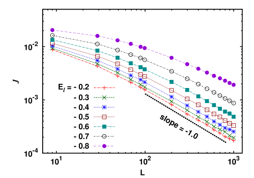
Figure 6: (Color online) Log-log plot of the steady state current $J$ vs. $L$ agrees well with Fourier law $J\sim L^{-1}$ for large $L$, but deviates for small $L$ values. The average energy of the two baths are $E_{l}$ and $E_{r}=E_{l}+\Delta E$ with $\Delta E=0.1$ and $\Delta t=1.0$.

Keeping this in mind, a suggestive phenomenological equation for the energy current can be written as

$$J=\kappa\frac{\Delta E}{L+\xi}$$ (28)

where $\kappa$ and $\xi$ are parameters which depend on $T,\Delta t$. As the temperature $T\to 0$, the correlation length of the spin chain $\xi\to\infty$, and consequently heat transport shows an apparent ballistic behavior. In the other limit, i.e. when $T$ is large and $\xi\to 0$, thermal transport in the system is diffusive.

Following Eq. (28), $\kappa$ and $\xi$ can be measured from the slope and intercept of the straight line $L=\kappa\frac{\Delta E}{J}-\xi$. In the inset of Fig. 7, we have shown $L$ against $\Delta E/J$ for different bath temperatures; all the curves are linear and the best fitted straight lines give respective $\kappa$ and $\xi$. Further, we observe that the parameters $\kappa$ and $\xi$ always maintain a fixed ratio with each other for any given $\Delta t$. This becomes evident from the collapse of $J$ versus $L/\kappa$ curves for different bath temperatures (see Fig. 7). This implies that $\kappa$ should have the same $T$ dependence as $\xi$. Since near $T=0$ the correlation length $\xi\sim T^{-1}$, we expect that $\kappa$ should also diverge inversely with $T$ in the limit $T\to 0$ . In fact, $\kappa$ is the conductivity of the system in the thermodynamic limit $L\gg\xi$ and its divergence at $T=0$ indicates that the system is near a critical point.

The behavior of $\kappa$ with temperature $T$ is shown in Fig 8. Close to $T=0$ the system relaxes extremely slowly and numerical studies in this limit become computationally expensive. One needs to go to extremely small temperatures to see the $T^{-1}$ divergence of $\kappa$, which could not be reached with the available computational resources. The inset of Fig. 8 shows that $\kappa$ vanishes linearly in the limit $\Delta t\to 0$, which can be understood as follows. The DTOE update of a spin $\vec{S}_{i}$ keeps the local energy $(\epsilon_{i-1}+\epsilon_{i})/2$ conserved, i.e., $d\epsilon/dt=0.$ Therefore, for finite $\Delta t$ we must have $\Delta\epsilon\sim(\Delta t)^{2}$ so that $\underset{\Delta t\to 0}{lim}\dfrac{\Delta\epsilon}{\Delta t}=0$. Again from Eq. (13) we have

$$J\sim\langle\Delta\epsilon\rangle\sim(\Delta t)^{2}.$$ (29)

Since $\xi$ diverges as $(\Delta t)^{-1}$ (from Eq. (19)) and the current in this limit $J\sim\frac{\kappa}{\xi},$ we have $\kappa\sim\Delta t$.

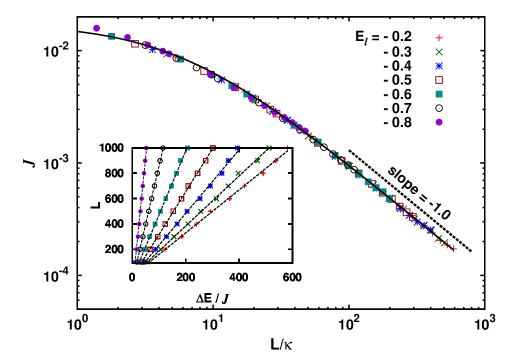
Figure 7: (Color online) Collapse of the curves $J$ vs $L/\kappa$ for different values of average bath energies $E_{l}$ and $E_{r}$ with a fixed $\Delta E=0.1$. The simulation data are shown by points and the solid line corresponds to the curve of the form $\dfrac{\Delta E}{(L/\kappa)+\xi/\kappa}$. The $\kappa$ values are obtained from a straight line fit of the form $L=\kappa\frac{\Delta E}{J}-\xi$ as shown in the inset (see text).

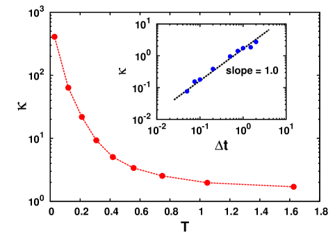
Figure 8: (Color online) Variation of $\kappa$ with temperature $T$, as obtained from the straight line fit using Eq. (28), shows a divergence in $\kappa$ as $T\to 0$. (Inset) $\kappa$ varies linearly with $\Delta t$.

Until now we have discussed thermal transport for a small $\Delta E$ and assigned the $\kappa$, obtained from Eq. (28), to be the conductivity of the thermodynamic system at energy $E$ (or temperature $T$). As such, in this limit the system is not too far from equilibrium, in a way that all parts of the system are maintained almost at the same temperature $T$. However if $\Delta E$ is appreciably larger, both local energy and its gradient varies significantly across the system. In such a case, one can appropriately define a local conductivity as,

$$\kappa_{local}=J{\left(\dfrac{d\epsilon(x)}{dx}\right)_{local}^{-1}}.$$ (30)

To measure $\kappa_{local}$, we set the bath energies at $E_{l}$ and $E_{r}\ll E_{l}$ and calculate the energy profile $\epsilon(x)$ and its gradient $\dfrac{d\epsilon(x)}{dx}$ at different $x=i/L$ along the system. The inset of Fig. 9 shows the energy profiles obtained for different bath energy $E_{l}$ and $E_{r}=E_{l}-0.5$. In the main figure, we have shown the local conductivity $\kappa_{local}$ as a function of the local energy $\epsilon(x)$; the overlapping regions, although obtained from energy profiles with different boundary energies, match remarkably. Thus $\kappa_{local}$ is a well defined function of the energy (or equivalently, temperature) and has the same value for a given energy, irrespective of the average energy of the two baths. Since the spin system attains local thermal equilibrium for all nonzero temperatures, $\kappa_{local}$ at a given local energy $\epsilon$ must be same as the conductivity $\kappa$ calculated using Eq. (28) for a large system with average bath energies $\epsilon$ and $\epsilon+\Delta E$ respectively. This is shown as open circles in Fig. 9 for $\Delta E=0.1,$ and different $\epsilon.$

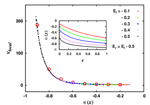
Figure 9: Variation of local conductivity $\kappa_{local}$ with energy $\epsilon(x)$. $\kappa_{local}$ has been calculated locally (from the profiles shown in inset) using Eq. (30). In the overlapping regions of the energy profiles, $\kappa_{local}$ for different energies collapses onto a single curve. As energy becomes small (which corresponds to $T\to 0$), the local conductivity diverges. The open circles correspond to $\kappa$ calculated using Eq. (28), $\Delta E=-0.1$, and for different $E_{l}=-0.2$ to $-0.9$ in steps of $-0.1$. For both the figures $\Delta t=1.0.$ and $L=1000$.

IV.5 Energy profiles

We now turn to the energy profile of the driven system and investigate the dependence of the same for the following three cases:

$\Delta t$ dependence.

The energy profile for a finite system depends on the parameter $\Delta t$ as can be seen from Fig. 10(a). We have shown earlier (see section IV C) that for finite $L$, the two asymptotic limits $\Delta t\to 0,\infty$ correspond to ballistic and diffusive transport respectively and hence it is expected that for a smaller $\Delta t$ the profile will be relatively flatter as compared to a larger value of $\Delta t$. Thus for any finite system if $L\ll\xi$ the transport will be ballistic (flat energy profile) and one has to simulate larger systems to observe a diffusive behavior (linear energy profile).

$E$ dependence.

A lower $E$ implies a lower temperature $T$ and hence for a given $L$ and $\Delta t$, the correlation length monotonically increases as $E$ is decreased. The system approaches a ballistic limit with energy profile as $E$ is reduced for a given value of $\Delta t$ and $L$. However in the thermodynamic limit and for $T>0$, Fourier law is always satisfied. This is shown in Fig. 10(b)

$L$ dependence.

The $L$ dependence of the energy profile is also consistent with what we have already discussed. For a given value of $\Delta t$ and $E$, a smaller $L$ shows a flatter profile as compared to a system with larger $L$, as can be seen from Fig. 10(c).

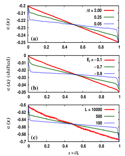
Figure 10: (Color online) Energy profiles for (a) different $\Delta t$ with fixed bath energies $E_{l}=-0.2$, $E_{r}=-0.25$ and $L=100$. (b) different bath energies $E_{l},E_{r}$ with $\Delta E=-0.05$, $\Delta t=0.1$ and $L=100$. The profiles have been shifted up along the energy axis by $|E_{l}|$ to accommodate all the profiles within the same energy window. (c) different $L$ with fixed bath energies $E_{l}=-0.6$, $\Delta E=-0.1$ and $\Delta t=0.1$.

V Discussion

To summarize, we have studied thermal transport in a one-dimensional classical Heisenberg spin model using discrete time parallel even-odd updates with spin precession (DTOE). While conventional integration schemes fail to preserve the required conservation of $S_{i}^{2}$ and $E$, this dynamics preserves both. The DTOE dynamics converts the equation of motion (2) to a map (Eq. (6)) with an additional parameter $\Delta t$ (besides the interaction strength $K$ and the system size $L$); the equation of motion is recovered from the map in the limit $\Delta t\to 0$. We explicitly show that this energy conserving dynamics equilibrates a closed system (having a fixed energy) and an open system attached to equal temperature heat baths, for any finite $\Delta t$. When the system is driven by maintaining a finite temperature difference between the two ends, we explicitly show that the system attains local thermal equilibrium. However, the steady state properties such as the correlation length $\xi$ (Eq. (19)), thermal current (Eq. (29)), and energy profile (Fig. 10 (a)) depend on $\Delta t$ when the system size $L$ is finite; such spurious $\Delta t$ dependence disappears in the thermodynamic limit.

Our numerical simulations of the system for different bath temperatures suggest that the thermal current $J$ can be expressed in the form $J=\kappa\frac{\Delta E}{L+\xi}$, where $\kappa$ and correlation length $\xi$ depend on the temperature $T$ and $\Delta t$. In the thermodynamic limit $L\gg\xi$, the spin system exhibits Fourier law; the energy profile in this case is linear with the slope asymptotically approaching the value $m^{*}=\frac{\Delta E}{L}.$ However, for small system sizes (i.e. for $L\ll\xi$), thermal transport appears to be ballistic with a relatively flatter energy profile. The same scenario prevails when, instead, the temperature $T$ is varied. That is, for a given $L$ and $\Delta t$, the slope of the energy profile approaches $m^{*}$ (or $0$) as $T\to\infty$ (or $0$). Thus, finite systems show an apparent crossover from a diffusive to a ballistic behavior as $T$ is lowered below a characteristic temperature scale $T^{*}$. This is described in Fig. 11 along with additional numerical evidences.

To demonstrate the crossover phenomena quantitatively, we measure the local slope $m$ of the energy profile at $i=L/2$ for a system of size $L$ and fit it to a functional form

$$m(T,\Delta t)=m^{*}\frac{T}{T+T^{*}(\Delta t)}.$$ (31)

Clearly, $T^{*}$ is the value of temperature for which the slope is half the desired slope for diffusive transport, $m^{*}=\frac{\Delta E}{L}.$ In Fig. 11 we show the crossover temperature $T^{*}(\Delta t)$ for two different system sizes, $L=100,200$. The crossover line $T^{*}(\Delta t)$ separates the diffusive regime (well above the curve) from the ballistic one (well below the curve). Again, the crossover line shifts downwards when the system size $L$ is increased. This clearly indicates that in the thermodynamic limit, the crossover line is infinitesimally close to the axes and thus, for any $T>0$, one observes a diffusive behaviour independent of the choice of $\Delta t.$ The apparent ballistic behaviour in the small $\Delta t$ or small $T$ regime is only an artifact of finiteness of the system and is a consequence of the divergence of the correlation length, as $\xi\sim 1/T$ and $\xi\sim 1/\Delta t$. The dependence of $\xi$ on $\Delta t$ can be understood from the fact that the spin precesses by a small angle, proportional to $\Delta t$. This effect is similar to a low temperature precession-dynamics, where the correlation length $\xi$ is very large. Thus, for studying thermal transport at a given $T$ and a small $\Delta t$, one must carefully choose the system size to be large enough such that the point ($\Delta t,T$) lies well above the crossover line.

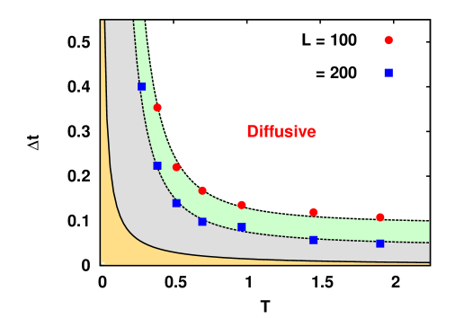
Figure 11: (Color online) The crossover line $T^{*}(\Delta t)$ in the $T$-$\Delta t$ plane for different $L$. In a finite system, this line separates the ballistic regime (shaded region below the curve), from the diffusive one. The data points are obtained numerically (see text) for $L=100,200$ (the broken line is only a guide to the eye). Following these trends, we schematically draw the same for very large $L$ (solid line). Evidently, the apparent ballistic behaviour disappears for $L\to\infty$ and one obtains Fourier law for all $T>0$, irrespective of the value of $\Delta t.$

The model is exactly solvable in both the limits $T\to 0$ and $T\to\infty$. In the $T\to 0$ limit, the thermal current $J=E_{l}-E_{r}$ is independent of $L$ and the energy profile $\epsilon(x)=\frac{1}{2}(E_{l}+E_{r})$ is flat. In this limit Fourier law is violated as $J$ is not proportional to local slope of $\epsilon(x)$, which is now zero since $\epsilon(x)$ is flat. The finite current $J=E_{l}-E_{r}$ is a consequence of the discontinuity of the energy profile at the boundaries. This discontinuity, and therefore a finite current, can never be obtained numerically for any finite $\Delta t$, however small. Numerical simulations, in fact, show that the current vanishes as $J\sim\Delta t^{2}$ for small $\Delta t.$

In the other solvable limit, i.e. when $T\to\infty$, however, the energy profile $\epsilon(x)=E_{l}+\frac{E_{r}-E_{l}}{L+2}x$ is linear and one obtains a finite thermal conductivity $\kappa=1$.

In conclusion, a thermodynamically large classical Heisenberg spin chain in one dimension obeys Fourier law for any non-zero temperature. However while studying thermal transport numerically for a finite system (though large) and a finite integration time step (though small) one must be careful in keeping the boundary temperatures larger than the characteristic scale $T^{*}(\Delta t,L)$ to obtain the correct thermodynamic behaviour. Otherwise, for $T\ll T^{*}$ the system will show an apparent ballistic behaviour which will eventually disappear in the $L\to\infty$ limit. This temperature dependent crossover from diffusive to ballistic behavior at small $T$ is expected since $T=0$ is a critical point with a diverging correlation length. It will be quite interesting to study thermal transport in a system where one can set the boundary temperatures such that a singular point falls in the bulk.

Acknowledgement : P.K.M. would thankfully acknowledge D. Dhar who initiated this work and suggested this energy-conserving dynamics, and M. Rao for fruitful discussions. The authors also wish to thank the anonymous referees for providing constructive comments.

References

- (1) F. Bonetto, J. L. Lebowitz, and L. Rey-Bellet, Fourier law: A challenge to theorists, in Mathematical Physics 2000, A. Fokas, A. Grigoryan, T. Kibble, and B. Zegarlinski, eds. (Imperial College Press, London, 2000), pp. 128150.
- (2) S. Lepri, R. Livi, and A. Politi, Phys. Rep. 377, 1 (2003).
- (3) A. Dhar, Advances in Physics, 57, 457, (2008).
- (4) R. Kubo, M. Toda, and N. Hashitsume, in Statistical Physics, Springer Series in Solid-State Science Vol. 2 ͑(Springer-Verlag, Berlin, 1991)
- (5) A. V. Savin, G. P. Tsironis, and X. Zotos, Phys. Rev. B 72, 140402(R) (2005).
- (6) R. W. Gerling and D. P. Landau, Phys. Rev. B 42, 8214-8219 (1990) and references therein.
- (7) K. Sakai and A. Klümper, J. Phys. A 35, 2173 (2002); J. Phys. A 36, 11617 (2003); X. Zotos, F. Naef and P. Prelovšek, Phys. Rev. B 55, 11029 (1997); J. Sirker, R. G. Pereira, and I. Affleck, Phys. Rev. B 83, 035115 (2011).
- (8) Hlubek et al, Phys. Rev. B 81, 020405 (2010)
- (9) F. Heidrich-Meisner, A. Honecker and W. Brenig, Eur. Phys. J. Special Topics 151, 135-145 (2007); C. Hess, Eur. Phys. J. Special Topics 151, 73 (2007); A. V. Sologubenko, T. Lorenz, H. R. Ott, and A. Freimuth, J. Low Temp. Phys. 147, 387 (2007).
- (10) Nonequilibrium Thermodynamics and Its Statistical Foundations, edited by H. J. Kreuzer (Clarendon Press, Oxford, 1981).
- (11) A. Dhar and D. Dhar, Phys. Rev. Lett. 82, 480 (1999).
- (12) Goldstein, Safko and Poole, Classical Mechanics, 3rd Edition, Addison Wesley.
- (13) G. S. Joyce, Phys. Rev. 155, 478 (1967)
- (14) V. Oganesyan, A. Pal and D. A. Huse, Phys. Rv. B 80, 115104͑ (2009)
- (15) H. Larralde, F. Leyvraz, and C. Mejia-Monasterio, J. Stat. Phys. 113, (2003) 197; C. Mejia-Monasterio and H. Wichterich, Eur. Phys. J. Spec. Top. 151, 113 (2007).
- (16) C. Kipnis, C. Marchioro, and E. Presutti, J. Stat. Phys., 27, 1 (1982).