Absorbing Phase Transition in Energy Exchange Models

Abstract

We study energy exchange models with dissipation ($\lambda$) and noise (of amplitude $\sigma$) and show that in presence of a threshold these models undergo an absorbing phase transition when either of dissipation or noise strength or both are varied. Using Monte Carlo simulations we find that the behaviour along the critical line, which separates the active phase from the absorbing one, belongs to Directed Percolation (DP) universality class. We claim that the conserved version with $\lambda=1$ and $\sigma=0$ also shows a DP transition; the apparent non-DP behaviour observed earlier is an artifact of undershooting in the decay of activity density starting from a random initial condition.

I Introduction

Absorbing state phase transitions (APT) DPbook ; book refer to a special class of non-equilibrium phase transitions which can occur in systems having absorbing configurations $i.e.$ configurations from which the system cannot escape dynamically. The most generic universality class of APT is the directed percolation (DP) DPbook ; book ; DP class. Several model systems, like reaction diffusion processes book , depinning transitions depinning , damage spreading spread , synchronization transition synchro and certain probabilistic cellular automata ca are known to undergo APT belonging to this universality class. In fact the famous ‘DP conjecture’ gras claims that any APT with a fluctuating scalar order parameter should generically belong to DP class. Recently the DP critical behaviour has been verified experimentally in context of liquid crystals DPexp .

APT in presence of a conserved field Rossi ; Heger has drawn a lot of attention in the past decade. Archetypical model of an APT with a conserved density field is the conserved lattice gas Rossi which shows a non-DP behaviour in 1-D Oliveira . In general, phase transitions in systems where activity is coupled to an additional conserved field are usually believed to belong to a universality class Rossi different from DP. However, there are several examples of systems belonging to DP irrespective of presence of a conserved field. Of them, probably the most important is the conserved Manna model Manna ; Dickman ; Lubeck . This model, though believed to show non-DP critical behaviour for a long time, has recently been claimed nomanna to belong to the DP class. Sticky sand-piles pk are notable instances of DP behaviour in presence of conserved fields. In this context it is worth mentioning a different class of models, the so called threshold driven energy exchange models which also show cclf_ws ; cclf APTs different from DP where activity is coupled to a conserved energy field.

In this article we introduce a generalised energy exchange model where the energy does not respect local conservation; dissipation $\lambda$ and noise amplitude $\sigma$ control the average energy of the system. The system shows an APT across a line of critical points $(\lambda_{c},\sigma_{c})$ which separates the active phase from the absorbing one in the $\lambda$-$\sigma$ plane. We show that the critical behaviour all along this critical line, including the special point $(\lambda=1,\sigma=0)$ where the dynamics is energy conserving, belongs to the directed percolation class. This claim that the conserved EEM belongs to DP, contradicts some recent studies of related models cclf_ws ; cclf . We argue that the apparent non-DP behaviour observed earlier is a consequence of unusually long transient effects arising due to the slow relaxation of the conserved background energy profile from random initial conditions (RIC). These ill effects are avoided here with the help of natural initial conditions nomanna ; natural . The natural initial condition is also advantageous in the non-conserved region $\lambda\simeq 1,\sigma\simeq 0,$ where the long transients associated with RIC still persist. However, as expected, these transient baheviour gradually disappears when dissipation is increased.

The article is organised as follows. In the next section we define the model and study the critical point $\lambda_{c}$ and critical exponents at a specific noise amplitude $\sigma=1$ in the section III. In section IV we explore the entire phase diagram in the $\lambda$-$\sigma$ plane. Section V is devoted to the special case of conserved EEM, where energy density plays the role of the control parameter.

II The Model

The model is defined on a periodic one dimensional lattice with $L$ sites labelled by $i=1,2,\dots L$; each site $i$ containing a positive real variable $E_{i}$ called energy. A pair of neighbouring sites is called active when at least one of the sites have energy larger than or equal to a predefined threshold $w$. Otherwise, $i.e.$ when both these sites have energy less than $w$, the pair is called inactive. The energies of an active pair ($i,i+1$) evolve following a random sequential update rule,

$$E_{pair}\to E_{pair}^{\prime} = \lambda E_{pair}+\xi~{};$$ (1)

$$E_{i}\to rE_{pair}^{\prime} ~{},~{} E_{i+1}\to(1-r)E_{pair}^{\prime},$$ (2)

where the sum of the energies $E_{pair}=(E_{i}+E_{i+1})$ is subjected to dissipation and noise, and $r\in(0,1)$ is a uniform random number. The parameter $0\leq\lambda\leq 1$ causes dissipation of the total energy. With an added random noise $\xi,$ chosen here from a uniform distribution in the range $(0,\sigma),$ the system mimics a dissipative particle system under the stochastic force stoch or the kinetic wealth exchange models of fluctuating markets ccm_epjb . Thus, like a canonical system in the influence of a Langevin bath, the average energy density is expected to be controlled by the parameters $\lambda$ and $\sigma.$

The interesting feature of this dynamics is that it allows the possibility of an absorbing state phase transition. A configuration where all the sites have $E_{i}<w,$ $i.e.$ none of the pairs are active, is an absorbing configuration of this system. Clearly, this system has infinitely many possible absorbing configurations. If the average energy density $e=\frac{1}{L}\sum_{i}E_{i}$ is much less than the threshold $w,$ the system is likely to fall in such a configuration. On the other hand for very large $e$ the system remains active. The energy density $e$ is a non-decreasing function of both the dissipation $\lambda$ and the noise amplitude $\sigma.$ Thus, for any given $\lambda<1,$ the average energy $e$ decreases as the amplitude $\sigma$ is decreased and one can expect an absorbing state phase transition at some critical value $\sigma_{c}(\lambda).$ For $\sigma>\sigma_{c}$ a thermodynamically large system reaches a steady state where number of active pairs in the system remains finite and for $\sigma\leq\sigma_{c}$ activity certainly dies out. Alternatively, one can study this transition by keeping $\sigma$ fixed and varying the dissipation factor $\lambda$ - in that case the transition occurs at a critical value $\lambda_{c}(\sigma).$

The critical curve $\lambda_{c}(\sigma)$ separates the active phase from the absorbing one in the $\lambda$-$\sigma$ plane. In a later section we will study this phase diagram. In the following we first study the critical behaviour of this system for a fixed noise amplitude, $\sigma=1,$ in some details. We shall find the critical point $\lambda_{c}$ and a set of the critical exponents using Monte Carlo simulations. Since the dynamics (2) is invariant under the transformation $(E_{i}\to\mu E_{i},\sigma\to\mu\sigma,w\to\mu w);$ we will work with $w=1$ without any loss of generality.

III Critical Behaviour for $\sigma=1$

The phase transition in this energy exchange model is characterized by the average density of active pairs $\rho_{a}=\langle\tau_{i}\rangle,$ where $\tau_{i}=1$ or $0$ depending on whether the pair $(i,i+1)$ is active or inactive. In the long time limit $\rho_{a}(t)$ saturates to a steady value, which is non zero only in the active phase; $\rho_{a}$ serves as the order parameter of this transition.

In this section we use Monte Carlo simulations to study the absorbing transition of the EEM. First let us expolore the critical point $\lambda_{c}$ and exponents for a fixed value of noise amplitude $\sigma=1.$

Critical point and $\alpha$: At the critical point $\lambda_{c},$ starting from a random initial condition, the activity density decays as a power law

$$\rho_{a}(t)\sim t^{-\alpha}.$$ (3)

One can estimate the critical point $\lambda_{c}$ and exponent $\alpha$ by plotting $\rho_{a}(t)$ versus $t$ for various values of $\lambda$ and looking for a power law decay. This estimate can be verified from the plot of $\rho_{a}(t)t^{\alpha}$ against $t;$ the curve corresponding to $\lambda=\lambda_{c}$ would remain constant in the long time limit. This procedure is illustrated in Fig. 1 which gives an estimate $\lambda_{c}=0.807122(2).$ The log scale plot of $\rho_{a}(t)$ at $\lambda_{c}$ gives an accurate estimate of the critical exponent

$$\alpha=0.159(1).$$

This is in very good agreement with the corresponding $\alpha_{DP}=0.15946.$

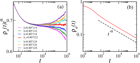
Figure 1: (Color online) Estimation of Critical point $\lambda_{c}$ for $\sigma=1$: (a) $\rho_{a}(t)t^{\alpha}$ versus $t$ curve for a system of size $L=10^{4}$ becomes constant in the large $t$ limit for $\lambda_{c}=0.807122.$ (b) Estimation of $\alpha=0.159(1)$ from $\rho_{a}(t)$ vs. $t$ plot for $\lambda=\lambda_{c}.$

Off-critical simulation and $\beta$: In the active phase the activity saturates to some finite value $\rho_{a}$ which vanishes algebraically as one approaches the critical point,

$$\rho_{a}\sim(\lambda-\lambda_{c})^{\beta}.$$ (4)

Here $\beta$ is the order parameter exponent. Figure 2(a) shows $\rho_{a}(t)$ as a function of $t$ for various values of $\Delta=\lambda-\lambda_{c}$ in the supercritical regime. Corresponding saturation values are plotted against $\Delta$ in log-log scale (see Fig. 2(b)); the slope of the resulting straight line gives us an estimate

$$\beta=0.278(2).$$

Again, this value of $\beta$ is consistent with the DP value $\beta_{DP}=0.2764.$

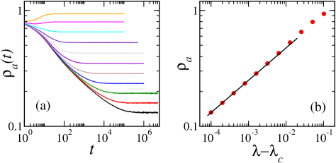
Figure 2: (Color online) Estimation of $\beta$ for EEM with $\sigma=1$: (a) Plot of $\rho_{a}(t)$ versus $t$ for different energy densities $\lambda>\lambda_{c}.$ (b) Corresponding saturation values plotted against $\Delta=\lambda-\lambda_{c}$ in double logarithmic scale; the slope corresponds to $\beta=0.278.$

Finite size scaling and $z$ : Next we turn our attention to the finite size scaling. For a finite system, the decay of $\rho_{a}(t)$ at the critical point is expected to follow the scaling forms

$$\rho_{a}(t) = t^{-\alpha}{\mathscr{G}}(t/L^{z}),$$ (5)

$$= L^{-\beta/\nu_{\perp}}\tilde{\mathscr{G}}(t/L^{z}),$$ (6)

where $\mathscr{G}$ and $\tilde{\mathscr{G}}$ are two different scaling functions. The dynamical exponent $z$ satisfies the scaling relation $\alpha z=\beta/\nu_{\perp}.$ At the critical point $\lambda=\lambda_{c},$ both the quantities $\rho_{a}(t)L^{\beta/\nu_{\perp}}$ and $\rho_{a}(t)t^{\alpha}$ for different values of $L$ are expected to collapse on to the corresponding unique scaling curve when plotted against $t/L^{z}.$ These data collapses, shown in Fig. 3(a) and (b) for systems of size $L=2^{8}$ - $2^{13},$ yield

$$z=1.59(1)\;\;{\rm and}\;\;\frac{\beta}{\nu}_{\perp}=0.25(1),$$

which are, again, in excellent agreement with the corresponding DP exponents. As expected, the estimates $\alpha,$ $z$ and $\beta/\nu_{\perp}$ satisfy the relation $\alpha z=\beta/\nu_{\perp}.$

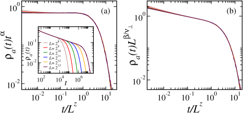
Figure 3: (Color online) Finite size scaling: (a) Plot of $\rho_{a}(t)t^{\alpha}$ as a function of the scaled variable $t/L^{z}$ for systems of sizes $L=2^{8},2^{9},\dots 2^{13}$ are collapsed using $z=1.59(1).$ The unscaled data are shown in the inset. (b) The same data could be collapsed following the scaling relation (5) when we use $\beta/\nu_{\perp}=0.25(1).$

All the estimated critical exponents $\alpha,\beta,z$ and $\beta/\nu_{\perp}$ match quite well with the corresponding DP values suggesting that the critical behaviour of the energy exchange model (at least for the noise amplitude $\sigma=1$) belongs to the directed percolation class.

III.1 The energy density

Next, we ask what happens to the energy density $e$ when the system undergoes a phase transition. Will this nonorder-parameter field $e(t)$ show the same power-law time dependence of $\rho_{a}(t),$ as seen in other models of APT Odor having infinitely many absorbing states ?

In the active phase the energy density $e(t)$ evolves along with $\rho_{a}(t),$ and saturates to a stationary value $e(\lambda,\sigma)$ in the long time limit. The critical value $e_{c}\equiv e(\lambda_{c},\sigma_{c})$ can be obtained from the decay of $e(t)$ as shown in Fig. 4(a) for $\lambda_{c}=0.807122$ and $\sigma_{c}=1.$ As $t\to\infty$ $e(t)$ saturates to a value $e_{c}=0.6452(4).$ We find that the reduced energy density $e(t)-e_{c}$ shows an algebraic decay $t^{-\tilde{\alpha}};$ this is illustrated in the inset of Fig. 4(a). A linear fit near the critical point yields

$$\tilde{\alpha}=0.158(1).$$ (7)

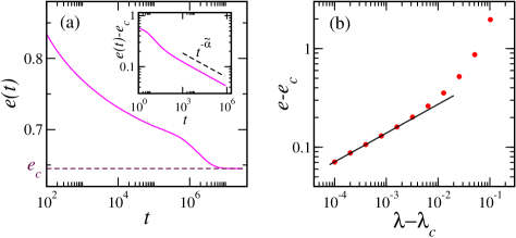
Figure 4: (Color online) (a) Plot of energy density $e(t)$ at $\sigma=1$ in the subcritical regime for different values of $\lambda=0.806322,0.806722,0.806922,0.807022$ and $\lambda_{c}.$ $e(t)$ saturates to $e_{c}=0.645$ at and below the critical point $(\lambda_{c}=0.807122,\sigma_{c}=1).$ The inset shows the corresponding log scale plot of $e(t)-e_{c};$ the slope, measured over last three decades, results in an estimate $\tilde{\alpha}=0.158(1).$ (b) The steady state values of the reduced energy $e-e_{c},$ plotted against $\lambda-\lambda_{c}$ for $\sigma_{c}=1,$ estimates $\tilde{\beta}=0.292(3).$

Clearly, within the error bars $\tilde{\alpha}$ is not different from $\alpha_{DP}=0.1594.$ This indicates that the reduced energy $e-e_{c}$ may be considered as an alternative order parameter of the APT in the EEM. To check whether the critical exponents of energy density indeed belongs to the DP class, we have also estimated the order parameter exponent $\tilde{\beta}.$ A plot of $e(\lambda)-e_{c}(\lambda_{c})$ against $\lambda-\lambda_{c}$ in log scale for $\sigma=1$ is shown in Fig 4(b); the slope of the straight line gives

$$\tilde{\beta}=0.292(3).$$ (8)

Once again, we find that $\tilde{\beta}\simeq\beta_{DP}.$ The other exponents like $z$ and $\beta/\nu_{\perp}$ for density are also found to be consistent with the corresponding DP values (data not shown here). Thus, the APT in EEM can also be characterized by a non-order parameter $e-e_{c}$ similar to some other models with infinitely many absorbing configurations Odor ; Mohanty .

IV Phase Diagram

The average energy of EEM is controlled by two parameters $\lambda$ and $\sigma.$ This gives rise to a phase diagram in the two dimensional $\lambda$-$\sigma$ plane where the active and inactive phases are separated by the line of critical points $(\lambda_{c},\sigma_{c}).$ We have used Monte Carlo simulations to trace this critical line in the phase plane. For a set of values of the noise amplitude $\sigma,$ we have estimated the critical point $\lambda_{c}$ using the procedure described in the previous section. These critical values $(\lambda_{c},\sigma_{c})$ are listed in the Table 1. The critical line, obtained by joining these points in the phase plane,is plotted in Fig 5(a). The shaded region $\sigma<\sigma_{c}(\lambda)$ corresponds to the absorbing phase of the system.

The phase diagram can also be drawn in the $e$-$\lambda$ plane eventhough $e$ is not an external tuning parameter. The steady state value of energy at the critical point $e(\lambda_{c},\sigma_{c})$ can be considered as the critical point $e_{c}$ for a given $\lambda=\lambda_{c}.$ The values of $e_{c}$ are also listed in Table 1 along with $(\lambda_{c},\sigma_{c}).$ Note that the statistical errors in the estimates of $e_{c}$ are comparatively large. Figure 5(b) shows the phase diagram in the $e$-$\lambda$ plane.

$\sigma_{c}$	$\lambda_{c}$	$e_{c}\equiv e(\lambda_{c},\sigma_{c})$
0.04	0.992117(1)	0.7372(2)
0.1	0.980089(1)	0.7228(2)
0.5	0.90000(2)	0.6736(4)
0.8	0.84305(1)	0.6536(4)
1	0.807122(2)	0.6452(4)
2	0.65113(1)	0.6089(4)
3	0.526988(4)	0.588(4)
4	0.42618(2)	0.569(2)
5.5	0.30667(1)	0.542(1)
7	0.21592(2)	0.515(3)
9	0.12808(2)	0.490(2)
11	0.06450(2)	0.454(1)
13.578(2)	0	0.378(1)
0	1	0.75243(3)

Table 1: Critical points of the $(1+1)$-dimensional energy exchange model. $e_{c}$ gives the average energy density at the critical point. The last row corresponds to the conserved case.

We have studied the decay of $\rho_{a}(t)$ for all these points (listed in Table 1) and find that the critical behaviour of EEM is consistent with DP-universality on the entire critical line. We have not reported these results in details here as they are only repetitions of the same excercise done in the previous section for $\sigma=1$.

Note that the critical line approaches the point $(\lambda=1,\sigma=0)$ as the noise amplitude $\sigma$ is decreased. This is expected as for $\sigma=0,$ the system always falls into an absorbing state for any $\lambda<1$ by continuously dissipating energy. In this case, when $\lambda=1,$ the energy is not disspated from the system and thus the dynamics becomes energy conserving; the total energy is fixed by the initial condition. To study the phase transition at this special point $(\lambda=1,\sigma=0)$ one must tune the conserved energy density $e.$ For the conserved system the background energy profile does not evolve rapidly. The fluctuations existing in random initial configurations persists for a long time and the relaxation of the system to the stationary state, where the energy profile is essentially flat, becomes very slow. A separate section is devoted for a careful study of this conserved EEM.

These transient effects are also pronounced in the vicinity of the special point $(\lambda=1,\sigma=0).$ For example, $\rho_{a}(t)$ shows an atypical decay from random initial conditions. In Fig. 6(a) we have plotted $\rho_{a}(t)$ versus $t$ curve for a set of points $(\lambda_{c},\sigma_{c})$ on the critical line. Evidently, the algebraic decay $\rho_{a}(t)\sim t^{-\alpha}$ starts at an increasingly longer timescale as $\lambda_{c}$ is increased. In particular, substantial numerical effort is required to study the critical behaviour near the conserved limit $\lambda_{c}=1$ which is reasonably reduced if one uses the so called natural initial conditions nomanna ; natural .

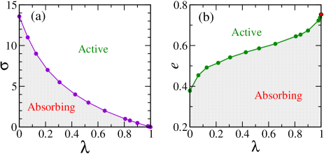
Figure 5: (Color online) (a) Phase diagram of EEM in the $\lambda$-$\sigma$ plane. The critical line separates the absorbing phase (shaded region) from the active one. (b) Corresponding phase diagram in the $\lambda$-$e$ plane. The point marked red corresponds to the critical energy of the conserved model.

Natural initial conditions are prepared by reactivating the steady state configurations. Thus, they have the same correlations . existing in the stationary state. For any value of the control parameter $(\lambda,\sigma),$ one usually starts from a random initial configuration and let the system evolve to the steady state. The natural initial states are then prepared from these steady state configurations by allowing the system to diffuse for a short time interval during which the energy of any randomly selected site, independent of whether it is active or not, is distributed unbiasedly among its neighbours. This process creates enough activity in the system so that one can observe the decay, but does not destroy the natural correlations built in the stationary state. Figure 6(b) shows a comparison of decay of activity starting from random (solid) and natural (dashed) initial conditions for two small values of $\sigma=0.04$ and $0.1$ for which this transient effect is most pronounced. Clearly, the curves corresponding to the natural initial condition reaches the scaling regime earlier than the same for random ones.

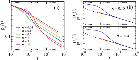
Figure 6: (Color online) (a) Decay of activity $\rho_{a}(t)$ at the critical point for random initial condition for different noise amplitude $\sigma.$ The power law behaviour starts at late times as $\sigma\to 0$ (or $\lambda\to 1$). (b) Comparison of $\rho_{a}(t)$ starting from random (blue solid line) and natural (black dashed line) initial conditions for two different noise amplitudes $\sigma=0.04$ (lower panel) and $\sigma=0.10$ (upper panel). The solid red line corresponds to slope $\alpha.$ The system size is $L=10^{4}.$

It is natural to expect that the conserved model ($\lambda=1,\sigma=0$) suffers worst from these ill-effects of random initial conditions. The need to use natural initial conditions will become more apparent in the next section where we turn our attention to this conserved energy exchange model and study APT by varying the conserved energy density $e.$

V The Conserved Energy Exchange Model

The dynamics of the EEM is energy conserving at the special point $(\lambda=1,\sigma=0)$ $i.e.$ when energy is neither dissipated nor added to the system as noise. In this case, the active pairs of neighbouring sites reshare their energies following,

$$E_{i} \to r(E_{i}+E_{i+1})$$ (9)

$$E_{i+1} \to (1-r)(E_{i}+E_{i+1})$$ (10)

where $r\in(0,1)$ is a uniform random number. Thus, the total energy does not evolve in time. This conserving dynamics have been studied in absence of a threshold ($i.e.$ when $w=0$) in different contexts of heat transport kipnis and Econo-physics yakovenko earlier. Like the non-conserved model, this conserved EEM also undergoes an APT but the control parameter here is the conserved energy density $e=\frac{1}{L}\sum_{i}E_{i}.$ Here too the density of active pairs $\rho_{a}$ plays the role of the order parameter and attains a non-zero stationary value only beyond some critical energy density $e_{c}.$

It has long been argued that absorbing transitions in presence of conserved fields Heger ; Lubeck belong to a universality class different from DP Rossi . But there are examples where an absorbing transition depicts DP behaviour even in presence of additional conserved fields pk ; nomanna . In this view, it is interesting to explore the critical behaviour of the special case $(\lambda=1,\sigma=0)$ of the energy exchange model.

First let us check whether $\rho_{a}(t)$ shows any unusual transient behaviour. We have measured the decay of activity $\rho_{a}(t)$ starting from random initial conditions, where the total energy is distributed randomly among all the lattice sites, for two different values of energy density $e$ which are shown as dashed lines in Fig. 7(a). The pronounced undershooting seen in these curves is an artifact of the disordered random initial conditions. As discussed in the previous section, one can avoid this long transient effect if ‘natural’ initial conditions are used. These initial conditions, prepared by taking the system to a stationary state and then allowing the energy to diffuse for a short time, lead to well behaved decay profile $\rho_{a}(t)$ (see solid lines in Fig. 7(a)). Since it is known that presence of undershooting in $\rho_{a}(t)$ may lead to erroneous estimation of the critical point and subsequent determination of critical exponents nomanna , in the following we study the APT of the conserved EEM using natural initial conditions.

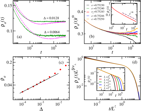
Figure 7: (Color online) Conserved EEM (a) Undershooting: Comparison of decay of $\rho_{a}(t)$ starting from random (dashed magenta) and natural (solid green) initial conditions for a system of size $L=10^{5}.$ (b) Determination of $e_{c}$: Plot of $\rho_{a}(t)t^{\alpha}$ versus $t$ for different values of $e;$ the horizontal curve corresponds to the critical point $e_{c}=0.75243.$ The inset shows log scale plot of $\rho_{a}(t)$ versus $t$ for $e=e_{c}$ with slope $\alpha=0.159.$ (c) Estimation of $\beta$: The saturation values of activity $\rho_{a}$ are plotted against $\Delta=e-e_{c}$ in double logarithmic scale; the slope corresponds to $\beta=0.283.$ (d) Finite size scaling: $\rho_{a}(t)L^{\beta/\nu_{\perp}}$ as a function of $t/L^{z}$ for different $L$ are collapsed using $z=1.58$ and $\beta/\nu_{\perp}=0.26.$ The inset shows the unscaled data.

Critical behaviour and exponents

First, let us estimate the critical point $e_{c}$ following the same procedure discussed in section III. The plot of $\rho_{a}(t)t^{\alpha}$ versus $t$ (shown for different $e$ in Fig. 7(b)) saturates in the long time limit for $e_{c}=0.75243(3).$ The $\rho_{a}(t)$ versus $t$ plot at this critical energy $e_{c}$ gives an estimate of the decay exponent

$$\alpha=0.159(2).$$

This value of $\alpha$ is consistent with $\alpha_{DP}.$

The order parameter exponent $\beta$ is determined from the steady state values $\rho_{a}$ of the activity in the active phase, as $\rho_{a}\sim(e-e_{c})^{\beta}.$ Figure 7(c) shows a plot of $\rho_{a}$ versus $\Delta=e-e_{c}$ in log-log scale; the slope of the resulting straight line gives us an estimate

$$\beta=0.283(4).$$

Again this value of $\beta$ is consistent with the DP value $\beta_{DP}=0.2764.$

The dynamical exponent $z$ and $\beta\nu_{\perp}$ are determined using the scaling form (5) by plotting $\rho_{a}(t)L^{\beta/\nu_{\perp}}$ against $t/L^{z}$ for different values of $L$ and looking for a data collapse. The best collapse is shown in Fig. 7(d) for systems of size $L=2^{8}$-$2^{12},$ and yields an estimate

$$z=1.58(2)~{}~{};~{}~{}~{}\frac{\beta}{\nu}_{\perp}=0.26(1)$$

which are, again, in excellent agreement with the corresponding DP exponents.

We find that all the critical exponents $\alpha,\beta,z$ and $\beta/\nu_{\perp}$ for the conserved energy exchange model agree quite well with the corresponding DP values. Thus this system provides another example where the presence of an additional conserved field does not a induce a different critical behaviour. It may be mentioned that the fixed energy sandpiles nomanna are known to be in DP class albeit having a conservation.

V.1 The Minimal Model

A variant of the energy exchange model has also been studied cclf_ws recently, where a pair of neighbouring sites randomly re-share their energies following the energy conserving dynamics (10) when at least one of them has energy less than or equal to the threshold $w.$ This model, henceforth referred to as the minimal energy exchange model, also undergoes an absorbing phase transition, apparently showing a non-DP behaviour cclf_ws . Since the minimal model has the identical local dynamics (10), it is natural to expect that its critical behaviour is same as the conserved EEM studied in Sec - V. The non-DP behaviour observed for the minimal model could have resulted from the long transients present in random initial conditions. In view of this we briefly revisit this model and study the critical behaviour using natural initial conditions.

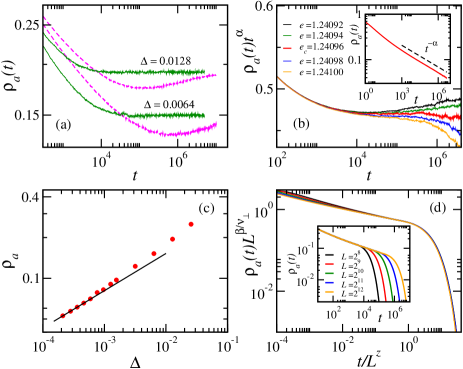
Figure 8: (Color online) Minimal conserved EEM (a) Undershooting: Comparison of $\rho_{a}(t)$ versus $t$ plot starting from random (dashed magenta) and natural (solid green) initial conditions; system size $L=10^{5}.$ (b) Critical point $e_{c}$: $\rho_{a}(t)t^{\alpha}$ versus $t$ curve for a system of size $L=10^{5}$ becomes constant for $e_{c}=1.24096$ as $t\to\infty.$ The inset shows estimation of $\alpha=0.159$ from $\rho_{a}(t)$ vs. $t$ plot. (c) Estimation of $\beta$: Saturation values of activity $\rho_{a}$ plotted as a function of $\Delta=e_{c}-e;$ the slope of the solid line corresponds to $\beta=0.275.$ (d) Finite size scaling: Data collapse according to Eq. (5) could be obtained when $z=1.54$ and $\beta/\nu_{\perp}=0.25.$ The inset here shows the unscaled data.

For completeness let us define the minimal model explicitly in one dimension. On a periodic lattice of size $L,$ each site $i$ has energy $E_{i}.$ A pair of neighbouring sites $(i,i+1)$ is said to be active when at least one of the sites $i$ or $i+1$ has energy less than or equal to a threshold value $w$, set to be unity. The active pairs in the model evolve following the energy conserving random sequential dynamics (10).

We proceed by defining the density of active pairs $\rho_{a}$ as the order parameter. The decay of activity $\rho_{a}(t)$ in the super critical regime, starting from the natural initial condition (solid line), is shown in Fig. 8(a) for two different values of average energy $e.$ Clearly $\rho_{a}(t)$ is well behaved and approaches to a stationary value reasonably fast. For comparison, in the same figure, we have included plot of $\rho_{a}(t)$ from the random initial condition (dashed line) for the same values of $e.$ Evidently, the pronounced undershooting in the random initial condition becomes stronger as one approaches the critical point. These effects may lead to inaccurate determination of $\alpha$ and $e_{c}$. Here we study the critical behaviour using natural initial condition.

Figure 8(b) illustrates the scheme for determination of the critical point which yields

$$e_{c}=1.24096(3).$$

This estimate of critical point $e_{c}$ is to be compared with $1/w_{c}$ reported in cclf_ws for the following reason. The minimal model was studied earlier with a fixed $e=1$ and varying the threshold $w.$ This resulted in a critical point $w_{c}=0.810$; in other words in the $(e,w)$ phase plane $(1,w_{c})$ is a critical point. It is evident that $(\lambda,\lambda w_{c})$ is also a critical point for any arbitrary $\lambda$ as both the conditional statement $E_{i}<w$ and the dynamics (10) are invariant under a scale transformation $(E_{i}\to\lambda E_{i},w\to\lambda w).$ This implies that the critical line in the $(e,w)$ phase plane is a straight line with unit slope passing through $(1,w_{c})$. Clearly $(1/w_{c},1)$ is also a critical point and it can be reached keeping $w$ fixed; thus of the minimal model along the line $w=1$ is expected to show the transition at $e_{c}=1/w_{c}$ when $e$ is tuned.

The critical point $e_{c}=1.24096(3)$ is slightly higher than the previously reported value $1/w_{c}=1.23456$ cclf_ws . We further show that this nominal correction in the estimate of critical point results in revised critical exponents which agree remarkably well with DP universality class.

The slope of the curve $\rho_{a}(t)$ versus $t$ in log scale (over last two decades) at the critical point $e_{c}$, shown in the inset of Fig. 8(b), gives an estimate of the exponent

$$\alpha=0.159(2),$$

which is in strikingly good agreement with $\alpha_{DP}.$

The stationary densities $\rho_{a}$ plotted against $e-e_{c}$ in log scale in Fig 8(c) results in an estimate

$$\beta=0.275(1),$$

which, again, matches well with $\beta_{DP}.$

The dynamical exponent $z$ and $\beta/\nu_{\perp}$ are obtained using the standard finite size scaling collapse following Eq. (5). Figure 8(d) shows this data collapse for $L=2^{8}-2^{12}$ using

$$z=1.54(2)~{}~{}~{}{\rm and}~{}~{}~{}\frac{\beta}{\nu}_{\perp}=0.25(1).$$

Both the estimates are in good agreement with the corresponding DP values.

To summarize, the critical exponents of the minimal model imply that, contrary to previous claims cclf_ws , the APT seen here, in fact, belongs to DP class. We must mention that the differences in the estimates of critical exponents found in this study are not in anyway related to the fact that the order parameter in Ref. cclf_ws was chosen differently. Instead of density of active pairs $\rho_{a}$, the average density of “sites having $E_{i}\leq w$” was used as order parameter. This order parameter $\rho=\langle s_{i}\rangle$, where $s_{i}=0$ when $E_{i}>w$ or otherwise $s_{i}=1,$ is related to $\rho_{a}$ as

$$\rho_{a}=\rho+\langle s_{i}(1-s_{i+1})\rangle.$$ (11)

Since $\rho_{a}$ is non-zero only when $\rho\neq 0$ and they are dimensionally identical, the critical point and corresponding exponents would be same in both cases.

VI Summary

In conclusion, we have studied absorbing phase transition in the energy exchange models in one spatial dimension. The dynamics of this model is controlled by two parameters - a noise of amplitude $\sigma$ and a dissipation factor $\lambda.$ The absorbing and active phases are separated by a critical line in the $\lambda$-$\sigma$ plane. With extensive Monte Carlo simulations we show that the critical behaviour of the energy exchange model belongs to directed percolation along the entire critical line. The critical line ends at the point $(\lambda=1,\sigma=0)$, where the dynamics is energy conserving. The numerical study of the critical behaviour suffers from long transients and unusual decay profiles when this conserved limit is approached. We show that this effect can be removed if one uses suitably prepared natural initial conditions.

The conserved EEM $(\lambda=1,\sigma=0)$ is special in a way that the conserved energy itself serves as the tuning parameter. This conserved version also suffers from the presence of long transients making it numerically hard to study the system using random initial conditions. Here again one can take advantage of the natural initial conditions which reaches the stationary state within a reasonably shorter time. We find that the critical behaviour of the conserved EEM also belongs to DP.

We also revisit the minimal energy exchange model (a variant of conserved EEM), and find that this model too shows DP critical behaviour. The apparent non-DP exponents found earlier cclf_ws are possibly due to the undershooting present in the decay of activity from the random initial conditions.

With this study we want to emphasize the fact that one has to be very careful in exploring absorbing phase transition in presence of a conserved field. The conserved field imposes additional constraints on the evolution of the system and introduces a long time scale. Random initial conditions may need very long time to saturate, producing unwanted transient effects like undershooting. These undesirable features may lead to erroneous estimation of critical point and hence inaccurate critical exponents. One must take care of these ill effects while studying APT in a system with a conserved field.

Acknowledgement: U.B. would like to acknowledge thankfully the financial support of the Council of Scientific and Industrial Research, India. (Grant No. SPM-07/489(0034)/2007).

References

- (1) M. Henkel, H. Hinrichsen, and S. Lübeck, Non-Equilibrium phase transitions, vol. 1, Springer, Berlin, (2008).
- (2) J. Marro and R. Dickman, Nonequilibrium phase transitions in lattice models, Cambridge University Press, Cambridge, (1999).
- (3) H. Hinrichsen, Adv. Phys. 49, 815 (2000).
- (4) F. D. A. A. Reis, Braz. J. Phys. 33, 501 (2003).
- (5) P. Grassberger, J. Stat. Phys. 79, 13 (1995).
- (6) M. A. Münoz and R. Pastor-Satorras, Phys. Rev. Lett. 90, 204101 (2003).
- (7) G. Ódor and A. Szolnoki, Phys. Rev. E 53, 2231 (1996).
- (8) H. K. Janssen, Z. Phys. B 42, 151 (1981); P. Grassberger, Z. Phys. B 47, 365 (1982).
- (9) K. A. Takeuchi, M. Kuroda, H. Chaté, and M. Sano, Phys. Rev. E 80, 051116 (2009).
- (10) M. Rossi, R. Pastor-Satorras, and A. Vespignani, Phys. Rev. Lett. 85, 1803 (2000).
- (11) S. Lübeck and P. C. Heger, Phys. Rev. Lett. 90, 230601 (2003); S. Lübeck and P. C. Heger, Phys. Rev. E 68, 056102 (2003).
- (12) M. J. de Oliveira, Phys. Rev. E 71, 016112 (2005).
- (13) S. Manna, J. Phys. A Math. Gen. 24, L363 (1991).
- (14) R. Dickman, M. Alava, M. A. Muñoz, J. Peltola, A. Vespignani, and S. Zapperi, Phys. Rev. E 64, 056104 (2001).
- (15) S. Lübeck, Int. J. Mod. Phys. B 18, 3977 (2004).
- (16) M. Basu, U. Basu, S. Bondyopadhyay, P. K. Mohanty, and H. Hinrichsen, Phys. Rev. Lett. 109, 015702 (2012).
- (17) P. K. Mohanty and D. Dhar, Phys. Rev. Lett. 89, 104303 (2002).
- (18) A. Ghosh, U. Basu, A. Chakraborti, and B. K. Chakrabarti, Phys. Rev. E 83, 061130 (2011).
- (19) M. Basu, U. Gayen, and P. K. Mohanty, arXiv:1102.1631.
- (20) I. Jensen and R. Dickman, Phys. Rev. E 48, 1710 (1993); G. Ódor, J. F. Mendes, M. A. Santos, and M. C. Marques, Phys. Rev. E 58, 7020 (1998); A. Lipowski and M. Droz, Phys. Rev. E 64, 031107 (2001).
- (21) R. Kubo, M. Toda and N. Hashitsume, Statistical Physics II : Non-equilibrium Statistical Mechanics, Springer, Heidelberg (1998).
- (22) U. Basu and P. K. Mohanty, Eur. Phys. J. B 65, 585(2008).
- (23) G. Ódor, J. F. Mendes, M. A. Santos, and M. C. Marques, Phys. Rev. E 58, 7020 (1998).
- (24) U. Basu and P. K. Mohanty, Eur. Phys. Lett., 99, 66002 (2012).
- (25) C. Kipnis, C. Marchioro and E. Presutti, J. Stat. Phys 27, 65 (1982).
- (26) A. Dragulescu, V. M. Yakovenko, Eur. Phys. J. B 17, 723 (2000).