Multiple $\Lambda$CDM cosmology with string landscape features
and future singularities

Abstract

Multiple $\Lambda$CDM cosmology is studied in a way that is formally a classical analog of the Casimir effect. Such cosmology corresponds to a time-dependent dark fluid model or, alternatively, to its scalar field presentation, and it motivated by the string landscape picture. The future evolution of the several dark energy models constructed within the scheme is carefully investigated. It turns out to be almost always possible to choose the parameters in the models so that they match the most recent and accurate astronomical values. To this end, several universes are presented which mimick (multiple) $\Lambda$CDM cosmology but exhibit Little Rip, asymptotically de Sitter, or Type I, II, III, and IV finite-time singularity behavior in the far future, with disintegration of all bound objects in the cases of Big Rip, Little Rip and Pseudo-Rip cosmologies.

I Introduction

Astronomical observations indicate that our Universe is currently in an accelerated phase Dat . This acceleration in the expansion rate of the observable cosmos is usually explained by introducing the so-called dark energy (for a recent review, see review ). In the most common models considered in the literature, dark energy comes from an ideal fluid with a specific equation of state (EoS) often exhibiting rather strange properties, as a negative pressure and/or a negative entropy, and also the fact that its action was invisible in the early universe while it is dominant in our epoch, etc. According to the latest observational data, dark energy currently accounts for some 73% of the total mass-energy of the universe (see, for example, Ref. Kowalski ).

In an attempt at saving General Relativity and to explain the cosmic acceleration, at the same time, one is led to conjecture some exotic dark fluids (although some other variants are still being considered, see e.g. vari1 ). Actually, General Relativity with an ideal fluid can be rewritten, in an equivalent way, as some modified gravity. Also, the introduction of a fluid with a complicated equation of state is to be seen as a phenomenological approach, since no explanation for the origin of such dark fluid is usually available. However, the interesting possibility that the dark fluid origin could be related with some fundamental theory, as string theory, opens new possibilities, through the sequence: string or M-theory is approximated by modified (super)gravity, which is finally observed as General Relativity with an exotic dark fluid. If such conjecture would be (even partially) true, one might expect that some string-related phenomena could be traceable in our dark energy universe. One celebrated stringy effect possibly related with the early universe comes from the string landscape (see, for instance, land ), which may lead to some observational consequences (see, e.g., mar ), since it could be responsible for the actual discrete mass spectrum of scalar and spinorial equations igor .

The equation of state (EoS) parameter $w_{\mathrm{D}}$ for dark energy is negative:

$$w_{\mathrm{D}}=p_{\mathrm{D}}/\rho_{\mathrm{D}}<0\,,$$ (1)

where $\rho_{\mathrm{D}}$ is the dark energy density and $p_{\mathrm{D}}$ the pressure. Although astrophysical observations favor the standard $\Lambda$CDM cosmology, the uncertainties in the determination of the EoS dark energy parameter $w$ are still too large, namely $w=-1.04^{+0.09}_{-0.10}$, to be able to determine, without doubt, which of the three cases: $w<-1$, $w=-1$, and $w>-1$ is the one actually realized in our universe PDP ; Amman .

The phantom dark energy case $w<-1$, is most interesting but poorly understood theoretically. A phantom field violates all four energy conditions, and it is unstable from the quantum field theoretical viewpoint, although it still could be stable in classical cosmology. Some observations hint towards a possible crossover of the phantom divide in the near past or in the near future. A very unpleasant property of phantom dark energy is the appearance of a Big Rip future singularity kam , where the scale factor becomes infinite at finite time in the future. A less dangerous future singularity caused by phantom or quintessence dark energy is the sudden (Type II) singularity barrow where the scale factor is finite at Rip time. Closer examination shows, however, that the condition $w<-1$ is not sufficient for a singularity occurrence. First of all, a transient phantom cosmology is quite possible. Moreover, one can easily construct models where $w$ asymptotically tends to $-1$ and such that the energy density increases with time, or remains constant, but there is no finite-time future singularity, what was extensively studied in Refs. kam ; Nojiri-3 ; barrow ; Stefanic ; Sahni:2002dx (for a review, see review , and for their classification, Nojiri-3 ). A clear case is when the Hubble rate tends to a constant (a cosmological constant or asymptotically de Sitter space), which may also correspond to a pseudo-Rip situation Frampton-3 . Also to be noted is the so-called Little Rip cosmology Frampton-2 , where the Hubble rate tends to infinity in the infinite future (for further details, see Frampton-3 ; LR ). The key point is that if $w$ approaches $-1$ quickly enough, then it is possible to have a model in which the time required for the singularity to appear is infinite, so that the singularity never forms in practice. Nevertheless, it can be shown that even in this case the disintegration of bound structures takes place, in a way similar to the Big Rip phenomenon. Such models are known as Little Rip and they have both a fluid and a scalar field description Frampton-2 ; As1 .

In the present paper we investigate a dark fluid model with a time-dependent EoS which can be considered as simple classical analog of the string landscape land_odin . The Casimir effect may lead to a similar picture. Some vacuum states appear which can be implemented with the help of the landscape. Moreover, we will study multiple $\Lambda$CDM cosmology as a classical analog of the Casimir effect (for a review see Caz1 ). This cosmology is also motivated by the string landscape picture. We demonstrate that such multiple $\Lambda$CDM cosmology may lead to various types of future universe, not only the asymptotically de Sitter one, but also to Little Rip cosmology and a finite-time future singularity, of any of the four known types Nojiri-3 . The equivalent description of multiple $\Lambda$CDM cosmology in terms of scalar theory is also further developed.

II Ideal fluid leading to multiple $\Lambda$CDM cosmology

Let us study the specific model of an ideal fluid which leads to a multiple $\Lambda$CDM cosmology. The corresponding FRW equations are

$$\frac{3}{\kappa^{2}}H^{2}=\rho\,,\quad-\frac{2}{\kappa^{2}}\dot{H}=p+\rho\,.$$ (2)

Here $\rho$ is the energy density and $p$ the pressure. Instead of (2), one can include the cosmological constant from gravity:

$$\frac{3}{\kappa^{2}}H^{2}=\rho+\frac{\Lambda}{\kappa^{2}}\,,\quad-\frac{2}{\kappa^{2}}\dot{H}=p+\rho\,.$$ (3)

We can, however, redefine $\rho$ and $p$ in order to absorb the contribution coming from the cosmological constant, namely,

$$\rho\to\rho-\frac{\Lambda}{\kappa^{2}}\,,\quad p\to p+\frac{\Lambda}{\kappa^{2}}\,.$$ (4)

With the redefinition (4), we re-obtain (2). Hence, it is enough to consider only the dark fluid in the FRW equation.

If $\rho$ and $p$ are given in terms of the function $f(q)$, with a parameter $q$ given by (compare with the similar Ansatz in land_odin ; grg )

$$\rho=\frac{3}{\kappa^{2}}f(q)^{2}\,,\quad p=-\frac{3}{\kappa^{2}}f(q)^{2}-\frac{2}{\kappa^{2}}f^{\prime}(q)\,,$$ (5)

the following solution of Eq. (2) is found

$$H=f(t)\,.$$ (6)

Note that the origin of time can be chosen arbitrarily. In (6), $t=q$ but one may choose $t=q+t_{0}$ with an arbitrary constant $t_{0}$. This shows that, besides the solution (6), $H=f(t-t_{0})$ can also be a solution.

If we delete $q$ in (5), we obtain a general equation of state (EoS):

$$F(\rho,p)=0\,.$$ (7)

In the case that $f^{\prime}(q)=0$ has a solution $q=q_{0}$, then there is a solution in which $H$ is a constant:

$$H=H_{0}\equiv f(q_{0})\,,$$ (8)

where $\rho=-p$, what corresponds to an effective cosmological constant. Then, if there is more than one solution satisfying $f^{\prime}(q)=0$, as $q=q_{n}$, $n=0,1,2,\cdots$, the theory could effectively admit several different cosmological constants, namely

$$H=f(q_{n})\,,\quad\Lambda_{n}=3f(q_{n})^{2}\,.$$ (9)

Note that, indeed, solutions (9) corresponding to different cosmological constants can exist simultaneously, which shows an interesting analogy with the cosmological landscape situation in string/M theory. Let us assume that, in fact, there is a solution corresponding to $q_{n}$. By perturbing this solution it may transit to another one, say $q_{n+1}$. The transition period will be proportional to $T_{n,n+1}=q_{n+1}-q_{n}$. This also hints to the possibility of occurrence of several $\Lambda$CDM phases in our observable universe.

III Example 1: Non-periodic behavior of the dark fluid

Consider the simplest case with two values of the cosmological constant

$$\dot{H}=q(\Lambda_{1}-t)(\Lambda_{2}-t)(1+\beta t)^{\gamma}\,,$$ (10)

where $q$, $\Lambda_{1}$, $\Lambda_{2}$, and $\gamma$ are constants. In this case the Hubble parameter takes the form ($\gamma\neq-1,\,-2,\,-3$)

$$H = q\frac{(1+\beta t)^{1+\gamma}}{\beta^{3}(1+\gamma)(2+\gamma)(3+\gamma)}$$

$$\times\left(2+\beta\left((3+\gamma)(\Lambda_{2}+\Lambda_{1}(1+\beta\Lambda_{2}(2+\gamma)))-(1+\gamma)(2+\beta(\Lambda_{1}+\Lambda_{2})(3+\gamma))t+\beta(1+\gamma)(2+\gamma)t^{2}\right)\right)\,.$$

It is easy to find the form of the scale factor ($\gamma\neq-4$)

$$a(t)=a_{0}\mathrm{e}^{q\frac{(1+\beta t)^{2+\gamma}\left(6+\beta\left((4+\gamma)(2\Lambda_{2}+\Lambda_{1}(2+\beta\Lambda_{2}(3+\gamma)))-(1+\gamma)(4+\beta(\Lambda_{1}+\Lambda_{2})(4+\gamma))t+\beta(1+\gamma)(2+\gamma)t^{2}\right)\right)}{\beta^{4}(1+\gamma)(2+\gamma)(3+\gamma)(4+\gamma)}}\,.$$ (12)

By choosing different values for the constants, the model will have different behaviors. Thus, if $\gamma>0$ then, for large values of time, the Hubble constant will be proportional to $t^{3+\gamma}$. If $\gamma<-4$ we have that $H\sim t^{3-|\gamma|}$. In addition, the constant $\beta$ can be either positive or negative. In the second case we obtain a singularity in the future: $a$ and $\rho$ go to infinity at finite time.

Suppose now that $\Lambda_{1}=0.1$ and $\Lambda_{2}=13.6$, at these points where we have an effective cosmological constant. The current value of the Hubble constant is known to be $H_{0}^{-1}=13.6$ Gyr. So one can find the value of the constant $q$. Now, choosing the value of $\gamma$, we can find $\beta$, the jerk parameter $j_{0}$ having been used in accordance with the observations. The deceleration parameter $q_{0}$ is $-1$, since at the current time we have a model with an effective cosmological constant. The calculated values of both the deceleration parameter $q_{0}$ and the jerk parameter $j_{0}$ can be found in Ref. Rapetti : $q_{0}=-0.81\pm 0.14$ and $j_{0}=2.16^{+0.81}_{-0.76}$ (from type Ia supernovae and X-ray cluster gas mass fraction measurements).

We choose, as an example of two parameter values for gamma: $\gamma=12$ and $\gamma=-5$. In the first case, in order for the jerk parameter to be in the permissible region, it is necessary that the parameter $\beta$ be in the range $0.00433706<\beta<0.00660997$. In the second case, we have that $-0.0228368<\beta<-0.0164559$. Thus, for this choice of constants, we have the following values of the cosmological parameters:

$$j_{0}=2.16^{+0.81}_{-0.76}\,,\quad q_{0}=-1\,,\quad H_{0}^{-1}=13.6\,\mathrm{Gyr}\,,\quad w=-1\,.$$

Assume that, at present, our model is approaching, or has already passed, the point corresponding to an effective cosmological constant. Let us set $\gamma=12$, then we can bring the model to the desired set up $q_{0}$ value. For $\Lambda_{2}<t_{0}$ one cannot choose the parameter $\beta$ in order to do the same.

Assume that $\Lambda_{2}=14$ ($t_{0}=13.6$). Then, the parameter $\beta$ has to take values in the range: $0.00637252351<\beta<0.006847247$. Thus, for this choice of constant, we have the following values for the cosmological parameters:

$$2.452<j_{0}<2.97\,,\quad-0.95>q_{0}>-0.932\,,\quad H_{0}^{-1}=13.6\,\mathrm{Gyr}\,,\quad-0.967<w<-0.955\,.$$

As we see, in this case $w>-1$.

Suppose now that $\gamma=-5$ and $\Lambda_{2}=14$ ($t_{0}=13.6$), then $-0.0222>\beta>-0.02364$, and we have the following cosmological parameters:

$$2.3915<j_{0}<2.45178\,,\quad-0.95>q_{0}>-0.92868\,,\quad H_{0}^{-1}=13.6\,\mathrm{Gyr}\,,\quad-1.06942<w<-1.0492\,.$$

Note that in this case $w<-1$ and we will have a Big Rip future singularity ($\rho$, $p$, $a\to\infty$) for $t$ in the range $42.2836<t<45.043$ (the lifetime of the universe).

Thus, for the chosen model (10) we have two possible scenarios for the evolution of the universe:

1. If $\gamma>1$, then the behavior of the EoS parameter $w$ is described in Fig. 2, and for $t\to\infty$ we have $w\to-1$ . In this case, for $t\to\infty$ we obtain that $H\to+\infty$ and we have a “Little Rip” Frampton-2 ; LR . As is known, bound objects in such universe disintegrate. One can estimate the time required for the solar system disintegration, the dimensionless internal force being

   $$F_{\mathrm{iner}}=\frac{\ddot{a}}{aH_{0}^{2}}\,.$$ (13)

   The Sun-Earth system disintegrates when $F_{\mathrm{iner}}\sim 10^{23}$ and we find this time to be $563.58$ Gyr (here $\Lambda_{1}=0.1$, $\Lambda_{2}=14$, $\beta=0.00637252351$, $\gamma=12$, and $q=0.0000184648$).

2. If $\gamma<-4$ then the behavior of EoS parameter is shown in Fig. 2 and we see that there is a singularity in the future at finite time (a Big Rip singularity), and $w\to-1$. After the singularity the Hubble constant will tend to zero, and the EoS state parameter will increase linearly. The lifetime of the universe that we find for the following values of the constants: $\Lambda_{1}=0.1$, $\Lambda_{2}=14$, $\beta=-0.023$, and $\gamma=-5$, $q=9.329681063413538\times 10^{-6}$, is $42.28<t<45.04$. In the same way one construct other examples of future evolution with Type II or Type III future singularity.

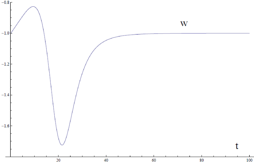
Figure 1: Plot of $w(t)$ ($0\leq t\leq 100$), for $\Lambda_{1}=0.1$, $\Lambda_{2}=14$, $\beta=0.00637252351$, $\gamma=12$, $q=0.0000184648$.

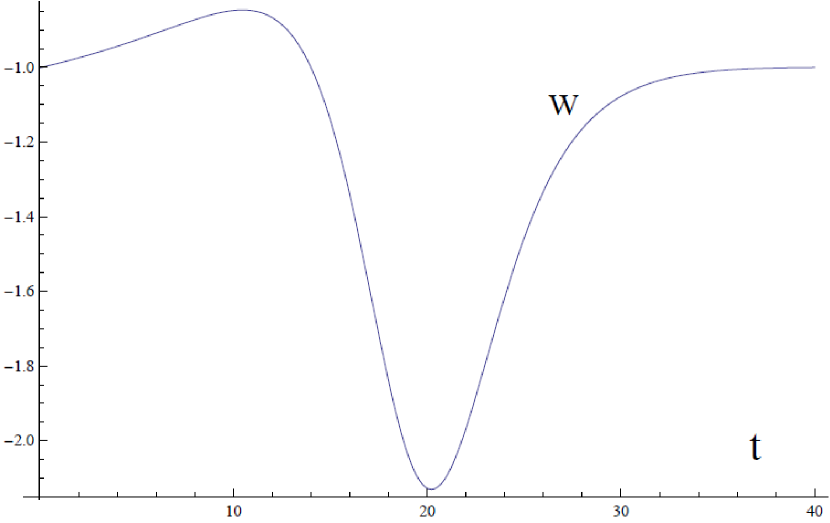
Figure 2: Plot of $w(t)$ ($0\leq t\leq 100$), for $\Lambda_{1}=0.1$, $\Lambda_{2}=14$, $\beta=-0.023$, $\gamma=-5$, $q=9.329681063413538\times 10^{-6}$.

IV Example 2: Periodic behavior of dark fluid

IV.1 The example of $\exp(\sin)$ dark fluid

As a second example, slightly different from the one above, consider the ideal fluid:

$$f(t)=H=H_{0}\mathrm{e}^{-g\left(t-\frac{1}{\omega}\sin\omega t\right)}\,,$$ (14)

which yields

$$f^{\prime}(t)=-H_{0}g\left(1-\cos\omega t\right)\mathrm{e}^{-g\left(1-\frac{1}{\omega}\sin\omega t\right)}\,.$$ (15)

In (14), it is assumed that $H_{0}$, $g$, and $\omega$ are constants. Therefore, $f^{\prime}(t)=0$ when $t=\frac{2\pi n}{\omega}$ for integer $n$. An effective multiple cosmological constant appears as

$$\Lambda_{n}=3H_{0}^{2}\mathrm{e}^{-\frac{4\pi ng}{\omega}}\,.$$ (16)

Again, $t=2\pi n/\omega$ corresponds to the cosmological constants in (14) and, therefore, the time-dependent solution could describe the transition between the cosmological constants, from the larger to the smaller one. In the limit of $t\to+\infty$ or $n\to+\infty$, the effective cosmological constant vanishes: $\lim_{n\to+\infty}\Lambda_{n}=0$. Now assume that, for $t=13.6$ Gyr, the Hubble constant is $13.6^{-1}$ Gy$r^{-1}$. We choose the parameters:

$$\omega=\frac{3\pi}{7}\,,\quad g=0.01\,,\quad H_{0}=0.084579\,,$$

for which we find the following values for the cosmological parameters:

$$j_{0}=2.21941\,,\quad q_{0}=0.980753\,,\quad H^{-1}=13.6\,\mbox{\rm Gyr}\,,\quad w=-0.987168\,.$$

The behavior of the Hubble constant is illustrated in Figs. 4 and 4. This is the “pseudo-Rip” case ($H\to H_{c}=0$, for $t\to\infty$). In other words, the universe is asymptotically de Sitter one. Nevertheless, due to the mild phantom behavior of the effective EoS parameter, it remains the possibility of dissolution of all bound objects sometime in the future.

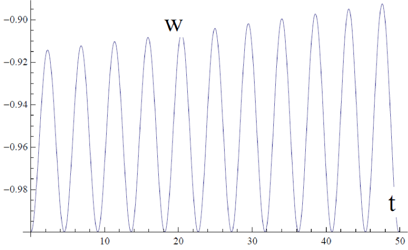
Figure 3: Plot of $w(t)$ ($0\leq t\leq 50$).

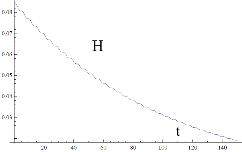
Figure 4: Plot of $H(t)$ ($0\leq t\leq 150$).

IV.2 The example $f(\sin)^{g}$ fluid

We now consider the following choice for $f(q)$,

$$f(q)=H_{0}\left(\frac{q}{t_{0}}-\sin\frac{q}{t_{0}}\right)\,.$$ (17)

Here $H_{0}$ and $t_{0}$ are positive constants. Then, using (6), we get the following solution:

$$H=H_{0}\left(\frac{t}{t_{0}}-\sin\frac{t}{t_{0}}\right)\,.$$ (18)

Since

$$\dot{H}=\frac{H_{0}}{t_{0}}\left(1-\cos\frac{t}{t_{0}}\right)\,,$$ (19)

there are de Sitter points, where $\dot{H}=0$, at $t=2n\pi t_{0}$, with $n$ an integer. When $t\neq 2n\pi t_{0}$, we find that $\dot{H}>0$ and, therefore, the universe is in a phantom phase. Since $H$ is finite for finite $t$, there is no Big Rip singularity, but $H$ goes to infinity when $t$ goes to infinity, that is, a Little Rip occurs.

One can alternatively consider the following $f(q)$,

$$f(q)=\frac{H_{0}}{\left(2N-1\right)\pi-\left(\frac{q}{t_{0}}-\sin\frac{q}{t_{0}}\right)}\,,$$ (20)

with $N$ a positive integer. Then, $H$ is given by

$$H=\frac{H_{0}}{\left(2N-1\right)\pi-\left(\frac{t}{t_{0}}-\sin\frac{t}{t_{0}}\right)}\,.$$ (21)

Again, we find de Sitter points at $t=2n\pi t_{0}$, with $n$ integer. However, when $t\sim\left(2N-1\right)\pi t_{0}$, instead of the de Sitter point, we get

$$H\sim\frac{H_{0}}{2\left(\left(2N-1\right)\pi-t\right)}\,,$$ (22)

which corresponds to a Big Rip singularity. Therefore, after the de Sitter point $t=2(N-1)\pi t_{0}$ or $n=N-1$, there is a Big Rip singularity and the universe does never reach the next de Sitter point $t=2N\pi t_{0}$.

We may consider more general forms for $f(q)$, as

$$f(q)=H_{0}\left\{\left(2N-1\right)\pi-\left(\frac{q}{t_{0}}-\sin\frac{q}{t_{0}}\right)\right\}^{\alpha}\,,$$ (23)

or

$$H=H_{0}\left\{\left(2N-1\right)\pi-\left(\frac{t}{t_{0}}-\sin\frac{t}{t_{0}}\right)\right\}^{\alpha}\,,$$ (24)

where $\alpha$ is a constant. Again, we find de Sitter points at $t=2n\pi t_{0}$, and for $t\sim\left(2N-1\right)\pi t_{0}$, we find

$$H\sim H_{0}\left\{2\left(2N\pi-t\right)\right\}^{\alpha}\,,$$ (25)

which corresponds to a Type I (Big Rip) singularity, when $\alpha\leq-1$, to a Type II one, when $0<\alpha<1$, to one of Type III, when $-1<\alpha<0$, and of Type IV, when $\alpha>1$ and $\alpha$ is not an integer. Already for the simple model above, the last de Sitter point before the Big Rip singularity appears at $t=2(N-1)\pi t_{0}$.

For the above examples it is not easy at all to write down the EoS explicitly, by deleting $q$ in (5), since the EoS obtained often becomes a multi-valued function. We should note, however, that it is easy to construct explicit models with a phantom scalar field to realize the above examples.

We may investigate the deceleration parameter $q_{0}$ and the jerk parameter $j_{0}$, which are defined as

$$q_{0}=-\frac{1}{aH^{2}}\frac{d^{2}a}{dt^{2}}=-1-\frac{\dot{H}}{H^{2}}\,,\quad j_{0}=1+\frac{3\dot{H}}{H^{2}}+\frac{\ddot{H}}{H^{3}}\,.$$ (26)

We now evaluate these quantities at the de Sitter points $t=2n\pi t_{0}$. For the model (18), we have $H=2n\pi H_{0}$ and $\dot{H}=\ddot{H}=0$, and we find $q_{0}=-1$ and $j_{0}=1$. For the rather simple models (22) and (24), we have already quite nice results: $\dot{H}=\ddot{H}=0$, therefore $q_{0}=-1$ and $j_{0}=1$. To wit, in the case of the $\Lambda$CDM model, these parameters are $q_{0}=-0.58$ and $j_{0}=1$. When the universe is not at a de Sitter point $t\neq 2\pi t_{0}$, the universe is in the phantom phase, where $\dot{H}>$, and therefore Eq. (26) tells us tht $q_{0}<-1$. Of course, we neglect the contribution from matter. If we include it, the universe could not be in the phantom phase at present, therefore we should obtain $q_{0}>-1$.

When we do include matter, the parameter $q$ in the EoS (5) cannot be identified with the cosmological time $t$ anymore. Since we have $f^{\prime}(q)$ and $f^{\prime\prime}(q)$ at the de Sitter point $q=q_{n}\equiv 2n\pi t_{0}$, one may imagine that $f(q)$ could be a constant $f(q)=f(q_{n})$ or

$$\rho=-p=\rho_{n}\equiv\frac{3}{\kappa^{2}}f(q_{n})^{2}\,.$$ (27)

Therefore, the fluid can be regarded as a (multiple) cosmological constant one. For matter we will now consider dust or cold dark matter and baryonic matter. If one of the de Sitter point corresponds to the present universe, the evolution of the universe can be approximated by the one corresponding to the $\Lambda$CDM model, and we have $q_{0}=-0.58$ and $j_{0}=1$. Let $H_{\mathrm{present}}$ be the present value of the Hubble rate, $H_{\mathrm{present}}\sim 70\,\mathrm{km}/\mathrm{s}\cdots\mathrm{Pc}$. If the present universe corresponds to the de Sitter point, we have

$$\frac{\kappa^{2}\rho_{n}}{3H_{\mathrm{present}}^{2}}=\frac{f(q_{n})^{2}}{H_{\mathrm{present}}^{2}}\sim 0.73\,,$$ (28)

which gives a constraint for the parameters of model. For example, for the model (17), we have

$$\frac{4\pi^{2}n^{2}H_{0}^{2}}{H_{\mathrm{present}}^{2}}\sim 0.73\,,$$ (29)

The deceleration parameter $q_{0}$ and the jerk parameter $j_{0}$ will not give any additional information on the relevant parameters. But if we had more accurate values of the snap parameter $s_{0}$ and of the jerk parameter $l_{0}$, which are defined as star

$$s_{0}=\frac{1}{H^{4}a}\frac{d^{4}a}{dt^{4}}\,,\quad l_{0}=\frac{1}{H^{5}a}\frac{d^{4}a}{dt^{5}}\,,$$ (30)

we could then obtain more constraints on the parameters $t_{0}$ and $n$.

As the universe expands, the relative acceleration between two points separated by a distance $l$ is given by $l\ddot{a}/a$. If there is a particle with mass $m$ at each of these points, an observer at one of the masses will measure an inertial force on the other mass, as

$$F_{\mathrm{iner}}=ml\ddot{a}/a=ml\left(\dot{H}+H^{2}\right)\,.$$ (31)

We may estimate the inertial force for the model (18). At late time, $t\gg t_{0}$, we find $H\sim\frac{H_{0}}{t_{0}}t$ and $H^{2}\gg\left|\dot{H}\right|$, therefore,

$$F_{\mathrm{iner}}\sim\frac{mlH_{0}^{2}}{t_{0}^{2}}t^{2}\,.$$ (32)

If the inertial force becomes larger than the binding energy for bound states, these bound states are ripped off and destroyed. This effect explains the disintegration of bound objects in rip universes (Big Rip, Little Rip or Pseudo-Rip).

Consider now the more general case

$$f(t)=H=\frac{q}{\left(1+c_{1}\left(t-b\sin\left(ct\right)\right)\right)^{g}}\,,$$ (33)

where $c$, $c_{1}$, $q$, $b$, and $g$ are constants. Then,

$$\dot{H}=c_{1}gq(-1+bc\cos(ct))\left(1+c_{1}t-b\,c_{1}\sin\left(ct\right)\right)^{-1-g}\,,$$ (34)

and it is easy to see that the time derivative of the Hubble constant will vanish periodically ($b\,c\,\cos(ct)=1$). We thus obtain a model with an effective cosmological constant $p=-\rho$. For the model (33), we have

$$w_{\mathrm{eff}}=-1-\frac{2c_{1}g\left(-1+b\,c\,\cos\left(ct\right)\right)\left(1+c_{1}\,t-b\,c_{1}\sin\left(ct\right)\right)^{-1+g}}{3q}\,.$$ (35)

Note that there is a large arbitrariness in the choice of the constants, since one can choose them so that the parameters strictly match their current values (see Fig. 5), and one can provide the required stages of the universe evolution: Accelerating primordial universe ($-1/3<w<-1$), deceleration of the universe ($-1/3<w<1/3$), and after that, when $w<-1/3$, the universe turns into an acceleration phase again. That is, a transition occurs from the accelerating to the decelerating phase, and back.

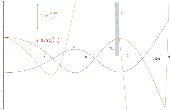
Figure 5: Plot of $j_{0}$ (green line), $-q_{0}$ (red line), and $w(t)$ (blue line), for $0\leq t\leq 20$, with $c_{1}=0.1$, $c=0.447$, $b=2.15$, $q=1.0445$, $g=3$. The lines of constant time determine the range of possible values, for the current time, of these quantities. The highlighted time interval corresponds to the values of $q_{0}$ and $j_{0}$ at present.

For $c_{1}=0.1$, $c=0.447$, $b=2.15$, $q=1.0445$, $g=3$, and $t=13.6$ Gyr we find the following values of the cosmological parameters: $q_{0}=-0.902$, $j_{0}=2.639$, $w=-0.935$, and $H_{0}=0.0752$ Gyr^-1. All these values correspond to the measured values at the current time ($t=13.6$ Gyr). Thus, with the pass of time both the cosmological constant and its derivative, and with them the energy density and pressure too, will tend to zero (see Figs. 7 and 7). One can easily see that $H\to 0$ for $t->\infty$ and, hence, those are pseudo-Rip models.

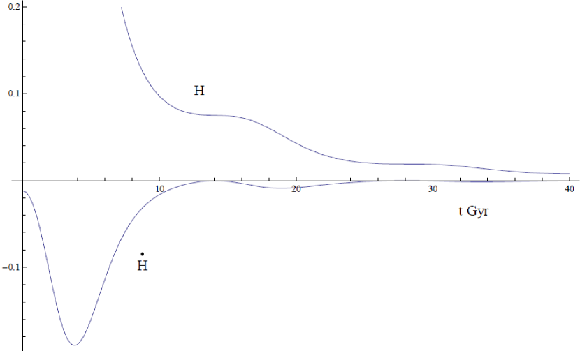
Figure 6: Plot of $H(t)$ and $\dot{H}(t)$.

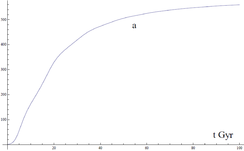
Figure 7: Plot of $a(t)$.

By selecting different values of the constants one can obtain different behaviors for the EoS parameter (see Fig. 9):

1. For the earlier values of time one gets accelerated expansion, then the expansion slows down, and later the acceleration will start again.

2. The oscillation $w$ can acquire values around minus one (see Fig. 9). This case corresponds to the Little Rip model ($H\to\infty$ for $t\to\infty$).

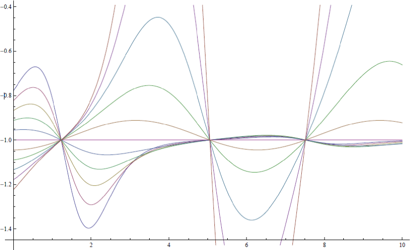
Figure 8: Plot of $w(t)$ ($0\leq t\leq 10$), for $c_{1}=1$, $c=0.1$, $b=3$, $q=3$, and $-5<g<5$.

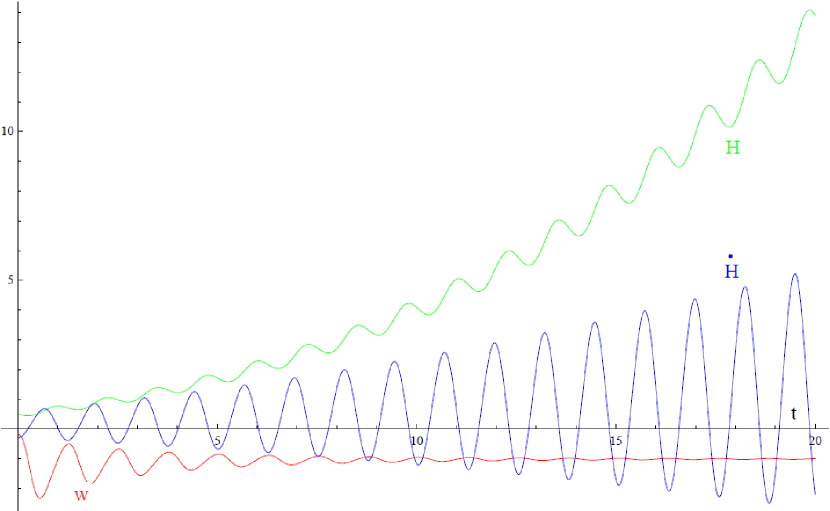
Figure 9: Plot of $H$ (green line), $w$ (red line), and $\dot{H}(t)$ (blue line), for $c_{1}=0.1$, $c=5$, $b=0.6$, $q=0.5$, and $g=-3$.

If $\gamma$ is positive and the parameter $c_{1}$ is negative, then we get a singularity in the future. This situation was already discussed above. By choosing proper values of the constants, different future singularities can be obtained as, for instance, the one depicted in Fig. 10.

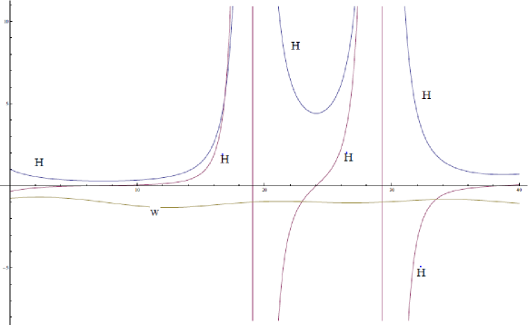
Figure 10: Typical behavior the model considered, for singularities of Big Rip type. In the present model, $g=2$.

It can be seen that a model of this kind leads to different types of evolution of the universe. First, one can build a model that will consistently describe all the stages in the universe evolution: accelerated expansion, slowing down to $w=1/3$, and accelerated expansion again, while for $t\to\infty$ the Hubble constant and its derivative tend to zero. Second, one can adjust for the right behavior of the model in the far future: The universe turns to be de Sitter or exhibits one of the four types of singularities. Moreover, almost always is it possible to choose the parameters so that they match the observed values. This is not difficult to do by assuming that at present the universe is in a phase corresponding to an effective cosmological constant. In addition, these models exhibiting multiple cosmological constants may coexist simultaneously, which definitely shows an analogy with the cosmological landscape picture.

V Cosmological reconstruction by one scalar model

We now construct scalar field models realizing the cosmological fluids given in the previous sections. The formulation is based on grg and we shall start with the following action:

$$S=\int d^{4}x\sqrt{-g}\left\{\frac{1}{2\kappa^{2}}R-\frac{1}{2}\omega(\phi)\partial_{\mu}\phi\partial^{\mu}\phi-V(\phi)+L_{\mathrm{matter}}\right\}\,.$$ (36)

Here, $\omega(\phi)$ and $V(\phi)$ are functions of the scalar field $\phi$. The function $\omega(\phi)$ is not relevant, as it can be absorbed into the redefinition of the scalar field $\phi$, as follows,

$$\varphi\equiv\int^{\phi}d\phi\sqrt{\left|\omega(\phi)\right|}\,.$$ (37)

The kinetic term of the scalar field in the action (36) has the following form:

$$-\omega(\phi)\partial_{\mu}\phi\partial^{\mu}\phi=\left\{\begin{array}[]{ll}-\partial_{\mu}\varphi\partial^{\mu}\varphi&\mbox{when $\omega(\phi)>0$}\\ \partial_{\mu}\varphi\partial^{\mu}\varphi&\mbox{when $\omega(\phi)<0$}\end{array}\right.\,.$$ (38)

The case $\omega(\phi)>0$ corresponds to quintessence or a non-phantom scalar field, and the case of $\omega(\phi)<0$ corresponds to a phantom scalar. Although $\omega(\phi)$ can be absorbed into the redefinition of the scalar field, we keep $\omega(\phi)$ since the transition between the quintessence and phantom cases can be best described by the change of sign of $\omega(\phi)$.

In order to consider and explain the cosmological reconstruction in terms of one scalar model, we rewrite the FRW equation as follows:

$$\omega(\phi){\dot{\phi}}^{2}=-\frac{2}{\kappa^{2}}\dot{H}\,,\quad V(\phi)=\frac{1}{\kappa^{2}}\left(3H^{2}+\dot{H}\right)\,.$$ (39)

Assuming $\omega(\phi)$ and $V(\phi)$ are given by a single function $f(\phi)$, as

$$\omega(\phi)=-\frac{2}{\kappa^{2}}f^{\prime}(\phi)\,,\quad V(\phi)=\frac{1}{\kappa^{2}}\left(3f(\phi)^{2}+f^{\prime}(\phi)\right)\,,$$ (40)

we find that the exact solution of the FLRW equations (when we neglect the contribution from matter) has the following form:

$$\phi=t\,,\quad H=f(t)\,.$$ (41)

It can be confirmed that the equation given by the variation over $\phi$,

$$0=\omega(\phi)\ddot{\phi}+\frac{1}{2}\omega^{\prime}(\phi){\dot{\phi}}^{2}+3H\omega(\phi)\dot{\phi}+V^{\prime}(\phi)\,,$$ (42)

is also satisfied by the solution (41). Then, the arbitrary universe evolution expressed by $H=f(t)$ can be realized by an appropriate choice of $\omega(\phi)$ and $V(\phi)$. In other words, defining the particular type of universe evolution, the corresponding scalar-Einstein gravity can be found.

For example, for the model (14), we get

$$\omega(\phi) = \frac{2H_{0}g}{\kappa^{2}}\left(1-\cos\omega\phi\right)\mathrm{e}^{-g\left(1-\frac{1}{\omega}\sin\omega\phi\right)}\,f^{\prime}(\phi)\,,$$

$$V(\phi) = \frac{1}{\kappa^{2}}\left(3H_{0}^{2}\mathrm{e}^{-2g\left(t-\frac{1}{\omega}\sin\omega\phi\right)}-H_{0}g\left(1-\cos\omega\phi\right)\mathrm{e}^{-g\left(1-\frac{1}{\omega}\sin\omega\phi\right)}\right)\,,$$ (43)

and, for the model (17),

$$\omega(\phi) = -\frac{2H_{0}}{\kappa^{2}t_{0}}\left(1-\cos\frac{\phi}{t_{0}}\right)\,,$$

$$V(\phi) = \frac{1}{\kappa^{2}}\left(3H_{0}^{2}\left(\frac{t}{t_{0}}-\sin\frac{t}{t_{0}}\right)^{2}+\frac{H_{0}}{t_{0}}\left(1-\cos\frac{t}{t_{0}}\right)\right)\,,$$ (44)

In the same way we can obtain the scalar theory corresponding to any of the other models described by a dark fluid with an EoS of the types considered above.

VI Conclusions

We have built in this paper several dark energy models, with a time-dependent equation of state, which can be viewed as simple classical analogs of the string landscape. The possible (simultaneous) existence of several cosmological constants can be interpreted as the possible presence of several vacuum states one has to choose from, what could bring into play Casimir effect considerations. Their simultaneous occurrence may indicate a future transition to a $\Lambda$CDM epoch with a different value for the effective cosmological constant.

It is very interesting to realize that the freedom we actually have in those models allows us in many cases, on top of providing a reasonable description of the different epochs of the universe evolution, to also adjust for their right behavior in the far future: the universe turns to be (asymptotically) de Sitter or exhibits one of the four types of finite-time future singularities or shows a Little Rip behavior. Moreover, up to some exceptions, it is possible to choose the parameters so that they match the astronomical data providing a very realistic description of $\Lambda$CDM cosmology. This is not difficult to do by assuming that, at the current moment of its evolution, the universe is in a phase corresponding to a given effective cosmological constant. Remarkably, the different models, which correspond to different cosmological constants, could coexist at the same moment, which definitely hints to an intriguing classical analogy with the cosmological landscape picture. From another viewpoint, the rich structure of the cosmological (singular) behavior of the models under discussion indicates that maybe similar phenomena could be typical in the string landscape.

The important lesson to be taken from current investigation is that, even if our current universe may look as the one described with the help of an effective cosmological constant, its finite-time future may be singular, so that its evolution might effectively end up. This opens the problem of the interpretation of the more precise observational data to come, which should be tailored with the specific purpose to understand what future is favored by the cosmological bounds this data will undoubtedly impose.

References

- (1) A. G. Riess et al. [Supernova Search Team Collaboration], Astron. J. 116, 1009 (1998) [astro-ph/9805201]; S. Perlmutter et al. [Supernova Cosmology Project Collaboration], Nature 391, 51 (1998) [astro-ph/9712212]; M. Hicken, W. M. Wood-Vasey, S. Blondin, P. Challis, S. Jha, P. L. Kelly, A. Rest and R. P. Kirshner, Astrophys. J. 700 (2009) 1097 [arXiv:0901.4804 [astro-ph]]; E. Komatsu et al. [WMAP Collaboration], Astrophys. J. Suppl. 180 (2009) 330 [arXiv:0803.0547 [astro-ph]]; W. J. Percival et al. [SDSS Collaboration], Mon. Not. Roy. Astron. Soc. 401 (2010) 2148 [arXiv:0907.1660 [astro-ph]].
- (2) K. Bamba, S. Capozziello, S. Nojiri and S. D. Odintsov, [arXiv:1205.3421 [gr-qc]].
- (3) M. Li, X. -D. Li, S. Wang and Y. Wang, Dark Energy, Commun. Theor. Phys. 56 (2011) 525 [arXiv:1103.5870 [astro-ph]].
- (4) M. Kowalski et al. [Supernova Cosmology Project Collaboration], Astrophys. J. 686, 749 (2008) [arXiv:0804.4142 [astro-ph]].
- (5) G. Cognola, E. Elizalde, S. Nojiri, S. D. Odintsov and S. Zerbini, JCAP 0502 (2005) 010 [hep-th/0501096]; E. Elizalde, S. Nojiri and S. D. Odintsov, Phys. Rev. D 70 (2004) 043539 [hep-th/0405034]; Y. -F. Cai, E. N. Saridakis, M. R. Setare and J. -Q. Xia, Phys. Rept. 493 (2010) 1 [arXiv:0909.2776 [hep-th]].
- (6) K. Nakamura et al. [Particle Data Group Collaboration], J. Phys. G G 37, 075021 (2010).
- (7) R. Amanullah, C. Lidman, D. Rubin, G. Aldering, P. Astier, K. Barbary, M. S. Burns and A. Conley et al., Astrophys. J. 716, 712 (2010) [arXiv:1004.1711 [astro-ph]].
- (8) R. R. Caldwell, Phys. Lett. B 545, 23 (2002) [astro-ph/9908168]; R. R. Caldwell, M. Kamionkowski and N. N. Weinberg, Phys. Rev. Lett. 91, 071301 (2003) [astro-ph/0302506].
- (9) S. Nojiri, S. D. Odintsov and S. Tsujikawa, Phys. Rev. D 71 (2005) 063004 [hep-th/0501025]; S. Nojiri and S. D. Odintsov, Phys. Rev. D 72 (2005) 023003 [hep-th/0505215].
- (10) J. D. Barrow, Class. Quant. Grav. 21 (2004) L79 [gr-qc/0403084].
- (11) H. Stefancic, Phys. Rev. D 71, 084024 (2005) [arXiv:astro-ph/0411630].
- (12) V. Sahni and Y. Shtanov, JCAP 0311, 014 (2003).
- (13) P. H. Frampton, K. J. Ludwick and R. J. Scherrer, Phys. Rev. D 84 (2011) 063003 [arXiv:1106.4996 [astro-ph]]; P. H. Frampton, K. J. Ludwick, S. Nojiri, S. D. Odintsov and R. J. Scherrer, Phys. Lett. B 708 (2012) 204 [arXiv:1108.0067 [hep-th]].
- (14) P. H. Frampton, K. J. Ludwick and R. J. Scherrer, Phys. Rev. D 85 (2012) 083001 [arXiv:1112.2964 [astro-ph]].
- (15) I. Brevik, E. Elizalde, S. Nojiri and S. D. Odintsov, Phys. Rev. D 84 (2011) 103508 [arXiv:1107.4642 [hep-th]]; P. H. Frampton and K. J. Ludwick, Eur. Phys. J. C 71 (2011) 1735 [arXiv:1103.2480 [hep-th]]; S. Nojiri, S. D. Odintsov and D. Saez-Gomez, [arXiv:1108.0767 [hep-th]]; L. N. Granda and E. Loaiza, Int. J. Mod. Phys. D 2 (2012) 1250002 [arXiv:1111.2454 [hep-th]]; P. Xi, X. -H. Zhai and X. -Z. Li, Phys. Lett. B 706 (2012) 482 [arXiv:1111.6355 [gr-qc]]; M. Ivanov and A. Toporensky, Int. J. Mod. Phys. D 21 (2012) 1250051 [arXiv:1112.4194 [gr-qc]]; M. -H. Belkacemi, M. Bouhmadi-Lopez, A. Errahmani and T. Ouali, Phys. Rev. D85, 083503 (2012); [arXiv:1112.5836 [gr-qc]]; A. N. Makarenko, V. V. Obukhov and I. V. Kirnos, [arXiv:1201.4742 [gr-qc]]; K. Bamba, R. Myrzakulov, S. Nojiri and S.D. Odintsov, Phys. Rev. D85, 104036(2012); Z. Liu and Y. Piao, Phys.Lett.B713,53 (2012).
- (16) A. V. Astashenok, S. Nojiri, S. D. Odintsov and A. V. Yurov, Phys. Lett. B 709 (2012) 396 [arXiv:1201.4056 [gr-qc]]; A. V. Astashenok, S. Nojiri, S. D. Odintsov and R. J. Scherrer, arXiv:1203.1976 [gr-qc].
- (17) L. Susskind, In Carr, Bernard (ed.): Universe or multiverse? 247-266 [hep-th/0302219]; M. R. Douglas, JHEP 0305 (2003) 046 [hep-th/0303194]; T. Banks, M. Dine and E. Gorbatov, JHEP 0408 (2004) 058 [hep-th/0309170].
- (18) M. Bastero-Gil, K. Freese and L. Mersini-Houghton, Phys. Rev. D 68 (2003) 123514 [hep-ph/0306289].
- (19) V. V. Kozlov and I. V. Volovich, [hep-th/0612135].
- (20) S. Nojiri and S. D. Odintsov, Phys. Lett. B 649 (2007) 440 [hep-th/0702031 [[hep-th]].
- (21) E. Elizalde, S. D. Odintsov, A. Romeo, A. A. Bytsenko and S. Zerbini, Zeta regularization techniques with applications, Singapore, Singapore: World Scientific (1994) 319 p. ; E. Elizalde, Ten physical applications of spectral zeta functions, 2nd Ed., Lecture Notes in Physics, (Springer-Verlag, Berlin, 2012); M. Bordag, G. L. Klimchitskaya, U. Mohideen and V. M. Mostepanenko, Int. Ser. Monogr. Phys. 145 (2009) 1; E. Elizalde, M. Bordag and K. Kirsten, J. Phys. A 31 (1998) 1743 [hep-th/9707083]; G. Cognola, E. Elizalde and K. Kirsten, J. Phys. A 34 (2001) 7311 [hep-th/9906228].
- (22) S. Nojiri and S. D. Odintsov, Gen. Rel. Grav. 38 (2006) 1285 [hep-th/0506212]; S. Capozziello, S. Nojiri and S. D. Odintsov, Phys. Lett. B 632 (2006) 597 [hep-th/0507182].
- (23) D. Rapetti, S. W. Allen, M. A. Amin and R. D. Blandford, Mon. Not. Roy. Astron. Soc. 375, 1510 (2007) [astro-ph/0605683].
- (24) V. Sahni, T. D. Saini, A. A. Starobinsky and U. Alam, JETP Lett. 77 (2003) 201 [Pisma Zh. Eksp. Teor. Fiz. 77 (2003) 249] [astro-ph/0201498].