Multiwavelet density estimation

Abstract

Accurate density estimation methodologies play an integral role in a variety of scientific disciplines, with applications including simulation models, decision support tools, and exploratory data analysis. In the past, histograms and kernel density estimators have been the predominant tools of choice, primarily due to their ease of use and mathematical simplicity. More recently, the use of wavelets for density estimation has gained in popularity due to their ability to approximate a large class of functions, including those with localized, abrupt variations. However, a well-known attribute of wavelet bases is that they can not be simultaneously symmetric, orthogonal, and compactly supported. Multiwavelets—a more general, vector-valued, construction of wavelets—overcome this disadvantage, making them natural choices for estimating density functions, many of which exhibit local symmetries around features such as a mode. We extend the methodology of wavelet density estimation to use multiwavelet bases and illustrate several empirical results where multiwavelet estimators outperform their wavelet counterparts at coarser resolution levels.

1 Introduction

Many applications require estimating the underlying probability density function (PDF) of a finite sample making minimal or no assumptions about the generating function. Having an accurate model of the underlying PDF enables one to understand the structure of the data and carry out more advanced statistical analysis such as classification, confidence modeling, and clustering. Here we introduce for the first time a new class of density estimators based on a series expansion of multiwavelets [2, 17]. Multiwavelets can be created to retain all of the desirable properties of regular wavelets and, in addition, exhibit very desirable properties which wavelets do not: simultaneous symmetry, compact support, and orthogonality. These properties make multiwavelet density estimation (MWDE) well-suited for reconstructing a wide class of density functions, particularly those that exhibit local or global symmetries.

The primary contribution of our work is to introduce for the first time the use of multiwavelets for density estimation. We also empirically compare MWDE performance to regular wavelet density estimation (WDE). Our focus is not to pit multiwavelets versus wavelets for the task of density estimation. We are still in the early stages of our research and continue to explore pros and cons associated with multiwavelets used as bases for density estimation. For example, the methodology we present here is strictly a linear multiwavelet estimator; hence, we do not discuss issues of thresholding the multiwavelet bases. Implementing an effective thresholding technique will yield sparser representations and should make MWDE more directly comparable to WDE. The richer mathematical properties afforded by multiwavelets demand we investigate their use for important applications such as density estimation.

1.1 Relevant Work

There are many well-studied density estimation techniques which we can loosely categorized into the taxonomy of parametric, semi-parametric, and nonparametric estimators. Of these, nonparametric models are the most data-driven, requiring little to no assumptions about the underlying generative model of the data. These models include the ubiquitous histogram described by Silverman [35] and the well-established kernel density estimators [32]. Though introduced in the 1960s by Čencov [6] and later described by Watson [45] and improved by Anderson and de Figueiredo [3], orthogonal series estimation (OSE) lagged in popularity due to lack of suitable bases for the series expansion. Despite this lag, work was done on OSE by Hall [19] and Ahmad [1] to investigate the convergence rate and integrated mean square error properties, respectively. Until about 25 years ago, the series expansions used for OSE were essentially limited to Fourier bases (i.e. sines and cosines) [22] or orthogonal polynomials, e.g. Hermite [31] and Laguerre [20]. The main downfall of these bases is their infinite support, demanding a large number of terms in the series expansion to accurately approximate complex densities containing multiple modes and abrupt variations. With the advent and growing use of wavelets, we are now seeing more uses of OSE [15, 30, 7, 5]. In fact, Peter and Rangarajan [28] show wavelet density estimators (WDE) often outperform many other nonparametric density estimators. The main advantage comes from the fact wavelets can be constructed with the convenient property of compact support [9], allowing them to easily and accurately represent functions with discontinuities and other abrupt local phenomena. In addition, WDE can be extended to non-linear estimators through the use of wavelet function coefficient thresholding introduced by Donoho et al. [11], which allows us to represent the density with a sparse set of coefficients while retaining accuracy.

Unfortunately, wavelets can not be simultaneously compact, symmetric, and orthogonal [9]. Many common analytic densities exhibit some form of symmetry either globally (e.g. Gaussian and Laplacian) or locally about their modes. The immediate consequence of wavelets lacking symmetry (if they also want to be orthogonal and compact) is that more of them will be required, either via a multiresolution expansion or a very fine single level expansion, to reproduce the symmetries in the underlying densities. Doing away with compactness and orthogonality allows us to have wavelet bases that are symmetric, but these relinquished features are the very properties that made wavelets an attractive choice over trigonometric or polynomial bases. This leaves us with only one choice of bases satisfying all these desirable properties: multiwavelets.

Multiwavelets are a more general, vector-valued construction of wavelets [2, 18, 17]. When used in a series expansion, they utilize multiple basis functions at every translate and at each resolution level. Like wavelets, multiwavelets can be constructed to have compact support, allowing them to faithfully model local discontinuities. Furthermore, they can be orthogonal, making coefficient estimation simple. Unlike wavelets, they can be symmetric while maintaining their compactness and orthogonality, allowing them to model local and global symmetries at coarser resolutions than wavelets. In this paper, we extend the concept of WDE to multiwavelet density estimation and demonstrate the utility of multiwavelets to model a variety of distributions. To our knowledge, this is the first use of multiwavelets for density estimation.

The remainder of this paper is organized as follows. The next section provides background knowledge of wavelets, WDE, and multiwavelets. In §3, we show how to construct a density estimator with multiwavelets. In §4, we demonstrate the capabilities of MWDE using a wide variety of multiwavelet families and compare MWDE to the conventional WDE. Finally, we conclude with some observations and directions for future research.

2 Review of Wavelets and Multiwavelets

2.1 Standard Wavelets and Multiresolution Analysis

Wavelets are refinable functions whose values are solutions to the dilation equation

$$\phi\left(x\right)=\sqrt{m}\sum_{k\in\mathbb{Z}}h_{k}\phi\left(mx-k\right),$$ (1)

where $\phi\left(x\right)$ is called the father wavelet (a.k.a. scaling function), $m\in\mathbb{Z}$ is the dilation factor (in our case, and in most practical cases, $m=2$), $h_{k}\in\mathbb{R}$ are low-pass coefficients (the “filter”) defining the wavelet, and $k$ are integer translates of the father wavelet across the domain. The dilation factor is further controlled by a choice of resolution level, $j\in\mathbb{Z}$, that expands or contracts the wavelet. Hence we will typically denote the normalized basis function at resolution $j$ and translate $k$ as $\phi_{j,k}=2^{j/2}\phi(2^{j}x-k)$. At a chosen resolution level $j$, the father wavelet and its integer translates form a basis for the function space $V_{j}$ which is a subspace of the space of all square integrable functions $L^{2}(\mathbb{R})$. These father wavelets capture the “smooth” or “averaging” properties of functions. Correspondingly, one can construct a set of mother wavelets which model the details (i.e. oscillating properties) of functions. These form a basis for the space $W{}_{j}$, which consists of functions orthogonal to $V_{j}$. The mother wavelets $\psi\left(x\right)$ (a.k.a. wavelet functions) are the members of $W$ and are found using the high-pass filter coefficients $g_{k}$ and by solving the wavelet, two-scale equation

$$\psi\left(x\right)=\sqrt{2}\sum_{k\in\mathbb{Z}}g_{k}\phi\left(2x-k\right).$$ (2)

Eqs. 1 and 2 only provide values for $\phi$ and $\psi$ evaluated on the dyadic rationals. If we want to evaluate $\phi\left(x\right)$ at any $x\in\mathbb{R}$, then we simply interpolate using known values of $\phi$ on the dyadic rationals. When this arises in the context of density estimation, we use a cubic spline interpolant.

There are several families of wavelets—Daubechies, Coiflets, Symlets, just to name a few—all of which are constructed from and defined by unique sets of coefficients. Wavelets can be constructed to have the convenient properties of orthogonality across their integer translates and compact support; however, these properties can not be had simultaneously with perfect symmetry [9]. As discussed in §2.3, this drawback can be addressed through the use of multiwavelets.

Scaling and wavelet bases can be brought together to represent functions in a multiresolution expansion. Given a function $f\in L^{2}\left(\mathbb{R}\right)$, a multiresolution analysis (MRA) of that function yields

$$f\left(x\right)=\sum_{k\in\mathbb{Z}}\alpha_{j_{0},k}\phi_{j_{0},k}\left(x\right)+\sum_{j=j_{0}}^{\infty}\sum_{k\in\mathbb{Z}}\beta_{j,k}\psi_{j,k}\left(x\right),$$ (3)

where $\alpha_{j_{0},k}\in\mathbb{R}$ are the father wavelet coefficients, and $\beta_{j,k}\in\mathbb{R}$ are the mother wavelet coefficients. The lowest resolution level used for function approximation is $j_{0}\in\mathbb{Z}$, and all other resolutions are $j\in\mathbb{Z}$ subject to $j\geq j_{0}$. In reality, though, only a finite set of resolutions will be utilized such that $j_{0}\leq j\leq J<\infty$. There are several approaches that can be applied for choosing $j_{0}$ and $J$; in the context of density estimation, we refer interested readers to Vidakovic [41]. The MRA in $L^{2}(\mathbb{R})$ is a doubly-infinite sequence of nested subspaces $V_{j\in\mathbb{Z}}$

$$\cdots\subset V_{-2}\subset V_{-1}\subset V_{0}\subset V_{1}\subset V_{2}\subset\cdots$$ (4)

such that $\bigcap_{j}V_{j}=\left\{0\right\}$ and $\overline{\bigcup_{j}V_{j}}=L^{2}(\mathbb{R})$, allowing $V_{j}$ to be used as a basis. The scaling and wavelet bases relationship is such that $W_{j}$ is orthogonal to $V_{j}$, and at any resolution level $j$ we have

$$V_{j}=V_{j-1}\oplus W_{j-1},$$ (5)

justifying the expansion in Eq. 3.

2.2 Wavelet Density Estimation

Wavelet density estimation is a specific incarnation of orthogonal series density estimation (OSE), where one expands the density function $p(x)$ in a multiresolution wavelet basis:

$$p\left(x\right)=\sum_{k\in\mathbb{Z}}\alpha_{j_{0},k}\phi_{j_{0},k}\left(x\right)+\sum_{j=j_{0}}^{\infty}\sum_{k\in\mathbb{Z}}\beta_{j,k}\psi_{j,k}\left(x\right).$$ (6)

The objective now becomes determining the coefficients $\alpha_{j_{0},k}$ and $\beta_{j,k}$ from a given independent and identically distributed (i.i.d.) sample $X=\left\{X_{i}\right\}_{i=1}^{N}$. The standard approach—though there are others [28]—is to simply project the density function onto the basis expansion:

$$\alpha_{j_{0},k}=\left\langle p,\phi_{j_{0},k}\right\rangle=\int p\left(x\right)\phi_{j_{0},k}\left(x\right)dx.$$ (7)

This allows us to interpret the inner product of Eq. 7 as an expectation to find

$$\alpha_{j_{0},k}=\int p\left(x\right)\phi_{j_{0},k}\left(x\right)dx=\mathcal{E}\left[\phi_{j_{0},k}\left(x\right)\right],$$ (8)

where $\mathcal{E}\left[\cdot\right]$ is the expectation operator. Assuming a finite sample, the expectation is approximated by the sample mean. Hence, the coefficients $\alpha_{j_{0},k}$ are estimated by

$$\hat{\alpha}_{j_{0},k}=\frac{1}{N}\sum_{i=1}^{N}\phi_{j_{0},k}\left(X_{i}\right),$$ (9)

and similarly for the wavelet function coefficients $\beta_{j,k}$ as

$$\hat{\beta}_{j,k}=\frac{1}{N}\sum_{i=1}^{N}\psi_{j,k}\left(X_{i}\right),$$ (10)

to arrive at the approximation $\hat{p}\left(x\right)$ given by

$$\hat{p}\left(x\right)=\sum_{k\in\mathbb{Z}}\hat{\alpha}_{j_{0},k}\phi_{j_{0},k}\left(x\right)+\sum_{j=j_{0}}^{J}\sum_{k\in\mathbb{Z}}\hat{\beta}_{j,k}\psi_{j,k}\left(x\right).$$ (11)

There are no guarantees, however, that the resulting density estimate $\hat{p}$ will satisfy the necessary properties of a density function (namely, $\int\hat{p}=1$ and $\hat{p}\geq 0$). So, once the density has been estimated, a post-processing normalization procedure [14] is typically performed to achieve these properties. It is worth noting there are ways to guarantee the resulting $\hat{p}$ is positive, such as using positive wavelets as in Walter and Shen [43], and even ways to ensure the resulting density will be positive and integrate to one, namely by estimating not $p$, but $\left(\sqrt{p}\right)^{2}=p$ with certain restrictions on the coefficients [29, 41, 28].

The utility of representing a density function using an MRA stems from the ability to threshold detail coefficients and gain an economical (in the sense of sparse coefficients), yet accurate estimator. These coefficients can be set to zero via “hard thresholding” techniques. Similarly, the larger mother wavelet function coefficients can be shrunk toward zero to reduce their contribution to the reconstruction, making the resulting estimate smoother; this is generally called “soft thresholding.” In Donoho et al. [11] and Donoho and Johnstone [10], thresholding and its implications on convergence are analyzed to provably show WDE to be optimal under mini-max criteria. When coefficient thresholding is employed, WDE is a class of nonlinear density estimators. Our present focus is to introduce the use of multiwavelets in density estimation. To this end, we do not address the issue of thresholding coefficients when using multiwavelets as the bases of our density estimator.

2.3 Multiwavelets

Multiwavelets are a more general, vector-valued constructions of wavelets. Excellent foundations of multiwavelet theory are given in Strela [38] and Keinert [21], with origins traced back to Alpert [2], Goodman et al. [18], and Goodman and Lee [17]. A multiscaling function $\underline{\phi}\left(x\right)$ is a vector-valued refinable function with multiplicity $r\in\mathbb{Z}^{+}$ of the form

$$\underline{\phi}\left(x\right)=\left(\begin{array}[]{c}\phi_{1}\left(x\right)\\ \vdots\\ \phi_{r}\left(x\right)\end{array}\right),$$ (12)

and satisfying the refinement equation

$$\underline{\phi}\left(x\right)=\sqrt{m}\sum_{k\in\mathbb{Z}}H_{k}\underline{\phi}\left(mx-k\right),\hskip 10.00002ptk,m\in\mathbb{Z},\hskip 10.00002ptm\geq 2,$$ (13)

where $H_{k}$ are low-pass $r\times r$ matrices called the “recursion coefficients” defining the multiscaling function and collectively referred to as the “multifilter,” paralleling the convention in standard wavelets. As before, we are concerned only with the dyadic case: $m=r=2$. In fact, all density estimations with multiwavelets presented in this paper are performed, for the sake of simplicity, with multiwavelets of multiplicity $r=2$. Multiscaling functions can be generated using a cascade algorithm of the same form as the standard wavelet cascade algorithm, but with matrix coefficients:

$$\underline{\phi}^{\left(n\right)}\left(x\right)=\sqrt{2}\sum_{k\in\mathbb{Z}}H_{k}\underline{\phi}^{\left(n-1\right)}\left(2x-k\right),$$ (14)

with an orthogonal $\underline{\phi}^{\left(0\right)}$, such as the Haar multiscaling function, paralleling the conventional Haar scaling function.

Mother multiwavelet functions $\underline{\psi}\left(x\right)$ (in this case, of multiplicity 2) can be created using the multiwavelet equation (paralleling Eq. 2 for standard wavelets):

$$\underline{\psi}\left(x\right)=\sqrt{2}\sum_{k\in\mathbb{Z}}G_{k}\underline{\phi}\left(2x-k\right),$$ (15)

where $G_{k}$ are high-pass $r\times r$ matrices.

Analogous to wavelets in §2.2, MRAs can be constructed for multiwavelets using the same procedure yielding the set $\left\{\underline{\psi}_{j,k}:j,k\in\mathbb{Z}\right\}$. This set is a basis for the space $W$. Like with traditional scalar wavelets, the multiscaling functions form a basis for the spaces $V_{j\in\mathbb{Z}}$, which are orthogonal to $W_{j\in\mathbb{Z}}$. As previously stated, we are not presently concerned with coefficient thresholding, so all multiwavelet density estimations in this paper are made using strictly multiscaling functions.

As with wavelets, there are many multiwavelet families—Shen-Tan-Tham (STT) by Shen et al. [34], Donovan-Geronimo-Hardin-Massopust (DGHM) by Geronimo et al. [16] and Donovan et al. [12] (with multiwavelet functions by Strang and Strela [37]), and Chui-Lan (CL) by Chui and Lian [8], just to name a few. Figs. 1, 2, and 3 illustrate the multiscaling and multiwavelet pairs for several well-known multiwavelet families. Like with standard wavelets, the properties of orthogonality and compact support are enforced during the construction of the recursion coefficients $H_{k}$ uniquely defining a multiwavelet. Unlike wavelets, however, multiwavelets can be simultaneously symmetric and compactly supported while retaining orthogonality across their integer translates. This desirable property serves as the primary motivation for density estimation with a multiwavelet basis rather than the standard wavelet basis.

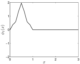
(a)

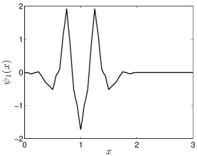
(b)

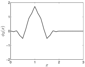
(c)

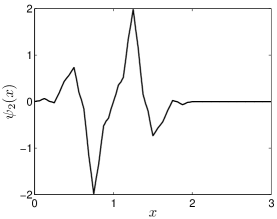
(d)

Figure 1: The DGHM multiwavelet has symmetric multiscaling functions Donovan et al. [12] and symmetric/antisymmetric multiwavelet functions Strang and Strela [37].

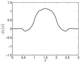
(a)

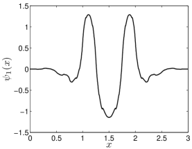
(b)

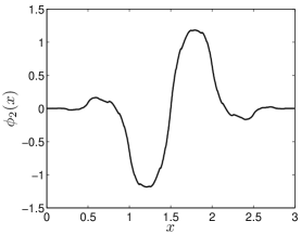
(c)

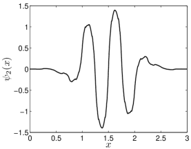
(d)

Figure 2: The STT multiwavelet Shen et al. [34] has symmetric/antisymmetric multiscaling and multiwavelet functions.

An interesting incarnation of multiwavelets are the so-called “balanced multiwavelets,” first explicitly introduced by Lebrun and Vetterli [23] and later more-rigidly formalized in Lebrun and Vetterli [24]. Selesnick [33] investigated the approximation properties of balanced multiwavelets, and later Lebrun and Vetterli [25] generalized the concept of multiwavelet balancing to arbitrarily high order. This class of multiwavelets was developed to solve a problem in signal-processing arising from the vector nature of multiwavelets, where a one-dimensional input signal must be vectorized before being passed through a multifilter. This vectorization can result in undesirable effects on the signal reconstruction due to “unbalanced” channels in the lowpass coefficients of the multifilter. Through procedures proposed by Lebrun and Vetterli [25], a multiwavelet can be balanced to eliminate these undesirable features of the lowpass coefficients. In fact, standard wavelets, such as the Daubechies, Symlets, and Coiflets, can be used to construct balanced multiwavelets. A particular balanced multiwavelet is shown in Fig. 3. Here, we have taken the standard Daubechies wavelet of order 2 and, with the toolkit from Keinert [21], used it to construct a balanced multiwavelet of multiplicity $r=2$. The resulting balanced multiwavelet is simply a compressed version of the original wavelet translated on the half-integers. We have illustrated this explicitly in Fig. 3 by showing the standard Daubechies wavelet on the first row and the components of the balanced multiwavelet on the remaining rows. We specifically mention balanced multiwavelets in this paper as they produce some interesting, though unsurprising, results when used as a basis for MWDE.

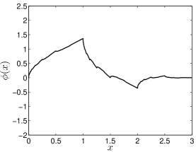
(a)

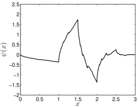
(b)

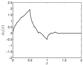
(c)

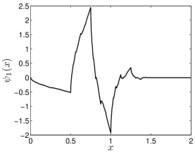
(d)

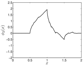
(e)

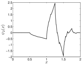
(f)

Figure 3: The standard Daubechies wavelet of order 2 is on the first row to illustrate that the balanced Daubechies multiwavelet (last two rows) is just compressed and translated versions of the standard Daubechies wavelet.

3 Multiwavelet Density Estimation

Our objective is to approximate a density function $p(x)$ using the multiwavelet basis in a form analogous to WDE. Again, the input is an i.i.d. sample of one-dimensional data $X=\left\{X_{i}\right\}_{i=1}^{N}$, and we aim to construct

$$p\left(x\right)=\sum_{k\in\mathbb{Z}}\underline{\alpha}_{j_{0},k}^{T}\underline{\phi}_{j_{0},k}\left(x\right)+\sum_{j=j_{0}}^{\infty}\sum_{k\in\mathbb{Z}}\underline{\beta}_{j,k}^{T}\underline{\psi}_{j,k}\left(x\right),$$ (16)

where, analogous to the wavelet case, $\underline{\varphi}_{j,k}\left(x\right)=2^{j/2}\underline{\varphi}\left(2^{j}x-k\right)$, where $\underline{\varphi}$ is $\underline{\phi}$ or $\underline{\psi}$. The coefficients $\alpha_{j_{0},k}$ and $\beta_{j,k}$ have become the $r$-dimensional vectors $\underline{\alpha}_{j_{0},k}$ and $\underline{\beta}_{j,k}$. We can expand Eq. 16 into its explicit vector form to see the reconstruction more clearly:

$$p\left(x\right)=\sum_{k\in\mathbb{Z}}\left(\begin{array}[]{c}\alpha_{1,j_{0},k}\\ \vdots\\ \alpha_{r,j_{0},k}\end{array}\right)^{T}\left(\begin{array}[]{c}\phi_{1,j_{0},k}\left(x\right)\\ \vdots\\ \phi_{r,j_{0},k}\left(x\right)\end{array}\right)+\sum_{j=j_{0}}^{\infty}\sum_{k\in\mathbb{Z}}\left(\begin{array}[]{c}\beta_{1,j,k}\\ \vdots\\ \beta_{r,j,k}\end{array}\right)^{T}\left(\begin{array}[]{c}\psi_{1,j,k}\left(x\right)\\ \vdots\\ \psi_{r,j,k}\left(x\right)\end{array}\right).$$ (17)

Evidently, the density function is completely described by the coefficients $\underline{\alpha}_{j_{0},k}$ and $\underline{\beta}_{j,k}$, so the objective is to estimate $\underline{\alpha}_{j_{0},k}$ and $\underline{\beta}_{j,k}$ as $\hat{\underline{\alpha}}_{j_{0},k}$ and $\hat{\underline{\beta}}_{j,k}$, respectively, using only the sample $X$. Before we detail a projection approach similar to WDE, it is worth expanding on the notion of orthonormality as it applies to multiwavelets to make explicitly clear the idea of multiwavelet density estimation in an OSE environment.

Multiwavelets are orthonormal across integer translates $k$ if

$$\left\langle\underline{\phi}\left(x\right),\underline{\phi}\left(x-k\right)\right\rangle=\int\underline{\phi}\left(x\right)\underline{\phi}^{*}\left(x-k\right)dx=\delta_{0k}I,$$ (18)

where $\delta_{ij}$ is the Kronecker delta function, $I$ is the $r\times r$ identity matrix, and $\underline{\phi}^{*}$ denotes the conjugate transpose of the vector $\underline{\phi}$. Note, that since $\underline{\phi}\in\mathbb{R}^{r}$ for our purposes, $\underline{\phi}^{*}=\underline{\phi}^{T}$. So, expanding Eq. 18, we find that

$$\int\left(\begin{array}[]{c}\phi_{1}\left(x\right)\\ \vdots\\ \phi_{r}\left(x\right)\end{array}\right)\left(\begin{array}[]{ccc}\phi_{1}\left(x-k\right)&\cdots&\phi_{r}\left(x-k\right)\end{array}\right)dx=\delta_{0k}\left(\begin{array}[]{ccc}1&&0\\ &\ddots\\ 0&&1\end{array}\right),$$ (19)

which implies

$$\left(\begin{array}[]{ccc}\int\phi_{1}\left(x\right)\phi_{1}\left(x-k\right)dx&\cdots&\int\phi_{1}\left(x\right)\phi_{r}\left(x-k\right)dx\\ \vdots&\ddots&\vdots\\ \int\phi_{r}\left(x\right)\phi_{1}\left(x-k\right)dx&\cdots&\int\phi_{r}\left(x\right)\phi_{r}\left(x-k\right)dx\end{array}\right)=\delta_{0k}\left(\begin{array}[]{ccc}1&&0\\ &\ddots\\ 0&&1\end{array}\right).$$ (20)

Finally, it is evident that

$$\int\phi_{i}\left(x\right)\phi_{j}\left(x-k\right)dx=\delta_{0k}\delta_{ij},$$ (21)

implying $\phi_{i}\left(x\right)$ is orthonormal to $\phi_{j}\left(x\right)$ when $i\neq j$ across integer translates $k$; that is, $\underline{\phi}$ can be constructed such that its elements are orthonormal across integer translates, justifying Eq. 16. The same conclusion holds for the mother multiwavelet functions. Therefore, we can calculate the coefficients $\underline{\alpha}_{j_{0},k}$ and $\underline{\beta}_{j,k}$ using the standard inner product projection:

$$\underline{\alpha}_{j_{0},k}=\left\langle p,\underline{\phi}_{j_{0},k}\right\rangle=\int p\left(x\right)\underline{\phi}_{j_{0},k}\left(x\right)dx,$$ (22)

and similarly for $\underline{\beta}_{j,k}$:

$$\underline{\beta}_{j,k}=\left\langle p,\underline{\psi}_{j,k}\right\rangle=\int p\left(x\right)\underline{\psi}_{j,k}\left(x\right)dx.$$

As before, this allows us to interpret the inner product in Eq. 22 as an expectation

$$\underline{\alpha}_{j_{0},k}=\int p\left(x\right)\underline{\phi}_{j_{0},k}\left(x\right)dx=\mathcal{E}\left[\underline{\phi}_{j_{0},k}\left(x\right)\right],$$ (23)

which is approximated as the sample mean

$$\hat{\underline{\alpha}}_{j_{0},k}=\frac{1}{N}\sum_{i=1}^{N}\underline{\phi}_{j_{0},k}\left(X_{i}\right).$$ (24)

The multiwavelet function coefficients $\underline{\beta}_{j,k}$ are estimated as expected:

$$\hat{\underline{\beta}}_{j,k}=\frac{1}{N}\sum_{i=1}^{N}\underline{\psi}_{j,k}\left(X_{i}\right).$$ (25)

The final approximation $\hat{p}\left(x\right)$ is given by

$$\hat{p}\left(x\right)=\sum_{k\in\mathbb{Z}}\hat{\underline{\alpha}}_{j_{0},k}^{T}\underline{\phi}_{j_{0},k}\left(x\right)+\sum_{j=j_{0}}^{J}\sum_{k\in\mathbb{Z}}\underline{\hat{\beta}}_{j,k}^{T}\underline{\psi}_{j,k}\left(x\right).$$ (26)

This is the linear multiwavelet density estimator. As in the wavelet case, nonlinear MWDE is also possible using either hard or soft thresholding of the multiwavelet coefficients $\hat{\underline{\beta}}_{j,k}$. For instance, see the work already done by [13, 40, 39] on multiwavelet coefficient thresholding in signals-processing applications. In addition to element-wise thresholding, Bacchelli and Papi [4] investigated vector-wise thresholding, taking advantage of the fact that multiwavelet coefficients can be correlated in their vector representations. As in WDE, the resolution levels $j_{0}\leq j\leq J<\infty$ are chosen by the user or by using model selection techniques as described, for instance, by Vidakovic [42]. We do not rigorously address the choice of resolution levels or coefficient thresholding here, as our objective is only to show that OSE can be successfully accomplished with multiwavelet bases.

4 Experimental Results

We detail several experiments using MWDE in comparison with standard WDE. We examine how multiwavelet symmetry can affect the reconstruction of densities with global and/or local symmetrical properties. Finally, we investigate the interesting case of using balanced multiwavelets. In addition to simple densities like the Gaussian, we extensively use the complicated density functions covered in Marron and Wand [26] and Wand and Jones [44]. These functions are, in many cases, multi-modal and contain local symmetries. We constructed a density estimator using various multiwavelet bases and measured the accuracy of the estimator under the integrated square error ($\mathrm{ISE}$) between the estimated density $\hat{p}$ and the actual density $p$. For the illustrated test cases, we use a variety of multiwavelet families chosen by their regularity of appearance in the literature. The multiwavelets were computationally constructed using the iterative cascading algorithm [36]. This is a standard procedure used even for wavelet constructions, with implementation details specific to multiwavelets available in Keinert [21].

4.1 Multiwavelet Symmetry

We begin by attempting to empirically motivate the advantages of MWDE versus WDE. Theoretically this was based on the fact that multiwavelets can be constructed with simultaneous symmetry, compact support, and orthogonality, whereas wavelets can not have these properties simultaneously. We developed a simple test to investigate the utility of the symmetry property by using multiwavelets and standard wavelets to estimate the symmetric unimodal Gaussian and a bimodal distribution. For this comparison, we employed the commonly-used Daubechies wavelet for the WDE. For multiwavelets, we have a choice of several symmetric and symmetric/antisymmetric families that have already been developed. The DGHM multiwavelet [12] has symmetric multiscaling functions and symmetric/antisymmetric multiwavelet functions [37]; it is plotted in Fig. 1. The STT multiwavelet [34] has symmetric/antisymmetric multiscaling and multiwavelet functions and is plotted in Fig. 2. We use both the DGHM and STT multiwavelets to demonstrate the capabilities of symmetric multiwavelets for density estimation. We do not employ any MRA for our density estimation, so the multiwavelet functions are not of direct interest here. However, such a density estimator could be easily constructed following the methodology detailed in §3.

First, we estimate a standard Gaussian density, as it has well-known properties, namely co-located mean/mode/median and symmetry. In Fig. 4, we show the DGHM multiwavelet outperforms the Daubechies wavelet of order 2 for resolution levels $-2\leq j\leq 0$, but at $j=0$, the Daubechies wavelet begins to produce a comparable estimate of the density, which continues to improve at finer resolutions. Given the highly asymmetrical properties of this lower-order Daubechies wavelet, the MWDE with a basis family such as DGHM was, as expected, able to outperform the WDE at some coarser resolution levels.

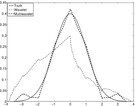
(a) $j=-2$

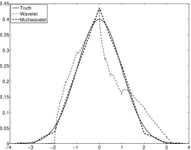
(b) $j=-1$

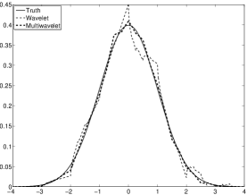
(c) $j=0$

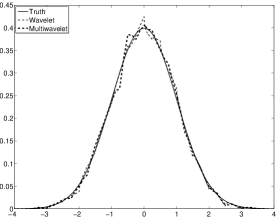
(d) $j=1$

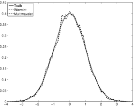
(e) $j=2$

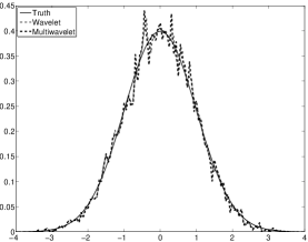
(f) $j=3$

Figure 4: MWDE of a symmetrical density (Gaussian with mean 0 and standard deviation 1) with 10000 samples across resolutions $-2\leq j\leq 3$ with the symmetric DGHM multiwavelet compared with WDE using the asymmetric Daubechies wavelet of order 2.

It is well-known that the Daubechies wavelet of order 2 is not necessarily well-suited for estimating smooth densities, such as the Gaussian distribution; this is evident from the jagged appearance of the wavelet. Similarly, the DGHM multiwavelet, though symmetrical, is also somewhat jagged in appearance. A more natural choice for estimating a smooth and symmetric density would be a higher-order wavelet, such as the Daubechies wavelet of order 5, and a smoother multiwavelet, such at the STT multiwavelet. With this, we compare WDE and MWDE using the more suitable bases just mentioned. The results are shown in Fig. 5. As anticipated, both the MWDE and the WDE are superior to the ones in Fig. 4. Even when using the Daubechies wavelet of order 5, we see that MWDE outperforms WDE at the coarse resolution levels $-2\leq j\leq 0$. At finer resolution levels $j>0$, we see, as in Fig. 4, the standard wavelet basis was able to produce a good density approximation. Being inherently symmetric, the multiwavelets are able to better reconstruct the symmetric peaks of these distributions, even at coarse resolutions. The standard wavelet resolutions must be increased to comparably model the symmetries.

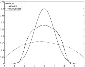
(a) $j=-2$

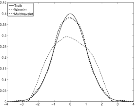
(b) $j=-1$

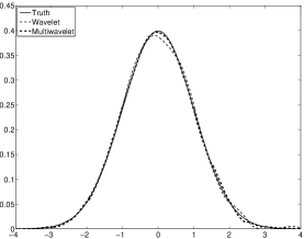
(c) $j=0$

(d) $j=1$

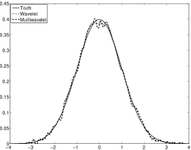
(e) $j=2$

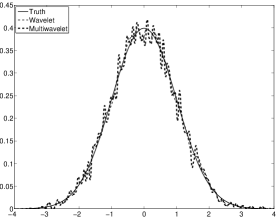
(f) $j=3$

Figure 5: MWDE of a symmetrical density (Gaussian with mean 0 and standard deviation 1) with 10000 samples across resolutions $-2\leq j\leq 3$ with the symmetric/antisymmetric STT multiwavelet compared with WDE using the asymmetric Daubechies wavelet of order 2.

4.2 Balanced Multiwavelets

From the work of Lebrun and Vetterli [24] and Lebrun and Vetterli [25], we know any wavelet can be used to construct a related balanced multiwavelet of arbitrarily high multiplicity. For instance, a Daubechies wavelet can be balanced to a Daubechies multiwavelet of multiplicity $r$, with $r$ multiscaling and $r$ multiwavelet functions. Balanced multiwavelets are of particular interest to us because they provide a somewhat-less subjective method of comparing WDE to MWDE. That is, we can compare MWDE using a balanced Daubechies multiwavelet to WDE using the Daubechies wavelet used to produce the balanced multiwavelet. The multiscaling and multiwavelet functions of balanced Daubechies multiwavelets turn out to be compressed and translated versions of the corresponding scaling and wavelet functions of the Daubechies wavelet [24]; this is evident from viewing Fig. 3.

MWDE with balanced multiwavelets possesses some interesting properties, especially for balanced Daubechies multiwavelets. Because balanced Daubechies multiwavelets are simply compressed and translated versions of their wavelet counterparts, we expect MWDE and WDE with these bases to be closely comparable. In fact, we find exactly this. We empirically observe a very interesting—if not expected—property where, if MWDE with balanced multiwavelets of multiplicity $r=2$ produces a certain reconstruction at some resolution level $j$, then the corresponding WDE “lags” the MWDE, and produces the same, or very close to the same, reconstruction at resolution $j+1$. This is clearly illustrated in Fig. 6, where we estimate a bimodal distribution with 10000 samples using the Daubechies wavelet of order 5 for WDE and the balanced Daubechies multiwavelet of order 5 for MWDE.

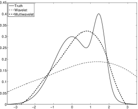
(a) $j=-2$

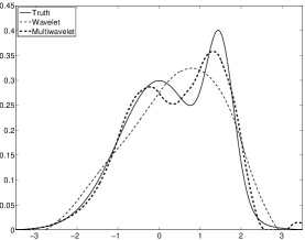
(b) $j=-1$

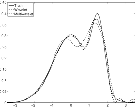
(c) $j=0$

(d) $j=1$

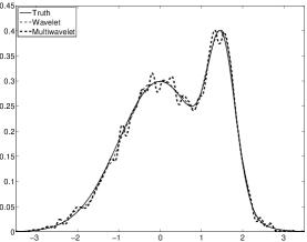
(e) $j=2$

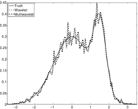
(f) $j=3$

Figure 6: WDE using Daubechies wavelet of order 5 and MWDE using balanced Daubechies multiwavelet of order 5 compared on a skewed bimodal distribution with 10000 samples at several resolution levels. Notice how the MWDE reconstruction at resolution $j=-2$ is very closely comparable to the WDE reconstruction at $j=-1$.

4.3 Other Multiwavelet Families

There are many families of multiwavelets available, and all the orthogonal families can be utilized for density estimation using the methods presented in this paper. To show the utility of MWDE, we estimated a broad range of densities from Marron and Wand [26] and Wand and Jones [44] using a variety of multiwavelet bases. Along with the MWDE, we show reconstructions using standard wavelet bases on the same plot; the WDE are presented here purely as benchmarks, not for pitting wavelets against multiwavelets. The results of these experiments are showcased in Fig. 7. It is worth noting that the WDE and MWDE are performed with the same resolution level in each density estimation plot. As we have seen in the previous two sections, the most evident difference in MWDE and WDE occurs when comparing across resolution levels. That is, MWDE tends to perform better than WDE at coarser resolutions.

We also conducted experiments using the cross product of all the multiwavelets available in Keinert [21] and the wavelets in Peter [27] (these wavelets and multiwavelets are listed in Tab. 1) across resolutions $-2\leq j\leq 3$ and for a variety of density functions from Marron and Wand [26] and Wand and Jones [44]. The parameters of the best (measured with $\mathrm{ISE}$) MWDE and WDE reconstructions of each density are shown in Tab. 2. The STT multiwavelet was the most successful multiwavelet for density estimation, as may be expected from its smooth appearance. In addition to the wavelet/multiwavelet families, resolution level, and $\mathrm{ISE}$ for each density, we also list the number of coefficients needed in the expansion to achieve the given result. Note here that no MRA (thus no thresholding) has been implemented, so the coefficient counts presented are simply the numbers of coefficients required by the basis to span the domain of the sample.

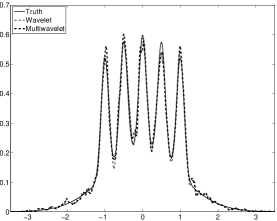
(a) Balanced Daubechies 6, Daubechies 6, $j=3$

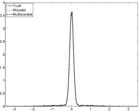
(b) DGHM, Coiflet 5, $j=4$

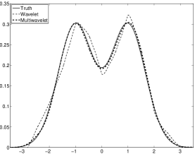
(c) Multisymlet 10, Symlet 4, $j=0$

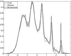
(d) Multisymlet 7, Daubechies 4, $j=2$

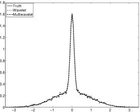
(e) DGHM, DMey, $j=3$

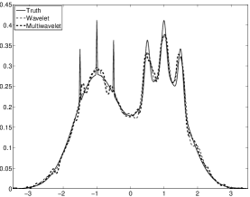
(f) STT, Coiflet 5, $j=2$

Figure 7: Various densities, each with 10000 samples, approximated with a variety of multiwavelets and wavelets to showcase the utility of MWDE alongside the familiar WDE presented purely as a benchmark. The multiwavelet family, wavelet family, and resolution level $j$ are provided, respectively, in each sub-figure.

Wavelet Families	Multiwavelet Families
Daubechies 2–10	Balanced Daubechies 2–10
Symlets 4–10	Multisymlets 4–10
Coiflets 1–5	Chui-Lian 2–3
Discrete Meyer	Bat
	DGHM
	STT

Table 1: Wavelet and multiwavelet families used in the density estimations in Tab. 2.

		MWDE			WDE
Density	ISE	Res.	Coeff.	ISE	Res.	Coeff.
	$(\times 10^{-3})$	$j$	#	$(\times 10^{-3})$	$j$	#
Normal	0.576	0	24	0.194	0	38
Bimodal	0.230	0	24	0.124	1	44
Skewed Bimodal	0.183	1	40	0.0997	1	46
Claw	1.25	3	128	0.659	3	90
Double Claw	1.67	2	64	1.33	3	85

Table 2: Results of estimating a variety of densities with both MWDE and WDE with several families of wavelets across resolutions $-2\leq j\leq 3$. Information about the density estimation with the lowest $\mathrm{ISE}$ is shown for both wavelets and multiwavelets. The wavelet and multiwavelet families used are listed in Tab. 1.

5 Discussion

We are motivated to investigate MWDE, for we can use symmetric and symmetric/antisymmetric bases, such as the STT and DGHM multiwavelets, instead of being limited to the necessarily asymmetric orthogonal wavelets. So, we began our investigation by comparing the results of using the DGHM multiwavelet for MWDE and the Daubechies wavelet of order 2 for WDE for estimating a symmetrical Gaussian distribution. As evident from Fig. 4, the DGHM multiwavelet outperforms the Daubechies wavelet at coarser resolution levels. Following this, we used the more suitable STT multiwavelet and Daubechies wavelet of order 5 to estimate the same density with much better results. The STT multiwavelet is much smoother than the DGHM multiwavelet, as is evident from comparing Figs. 1 and 2. We see in Fig. 5 that both the MWDE and WDE perform well, particularly at resolutions $j=0$ and $j=1$, respectively. The primary point of this empirical result is that the MWDE performed its best at a coarser resolution level than the wavelet. We will find this is a recurring theme throughout the tests we performed. This is an interesting relationship, one which we will continue to explore and develop more formally in later works.

We also investigated a specific and interesting class of multiwavelets: the so-called “balanced multiwavelets.” We tested MWDE using balanced multiwavelet bases and display the results in Fig. 6. The objective of this exercise was to examine the relationship across resolution levels between MWDE and WDE using related bases. As shown by Lebrun and Vetterli [24], we can balance a standard Daubechies wavelet to a balanced Daubechies multiwavelet. We did this using the Daubechies wavelet of order 5 balanced to a multiwavelet of multiplicity 2. We then compared across resolutions the density estimations resulting from using the Daubechies wavelet of order 5 for WDE and the balanced Daubechies multiwavelet of order 5 for MWDE. We found that MWDE and WDE result in very similar density estimates, but the wavelet “lags” the multiwavelet. That is, the MWDE at resolution level $j$ is very close to the WDE at resolution $j+1$. This is expected in the case of Daubechies wavelets because the balanced Daubechies multiwavelets are just compressed and translated on the half-integers versions of the the base Daubechies wavelet. We demonstrated this in Fig. 3.

There are, of course, many wavelet and multiwavelet families available with the necessary properties—namely orthogonality—for density estimation using the methods presented in this paper. We performed MWDE and WDE using a variety of multiwavelet and wavelet families on a broad sample of distributions and across several resolution levels. Our results are summarized in Tabs. 1 and 2. We consistently see the STT multiwavelet and Coiflet 5 wavelet perform the best under the $\mathrm{ISE}$. What is perhaps more interesting are the numbers of coefficients required in the various expansions to produce the density estimations. These are explicitly given in Tab. 2. As we have not used any non-linear density estimation, the numbers of coefficients presented are simply the numbers of coefficients required for the scaling and multiscaling functions to span the sample (which, in most cases, is contained on the unitless interval $\left[-4,4\right]$). From the table, we see that WDE, under the $\mathrm{ISE}$, provides the best density estimation for the given distributions. However, in most cases, MWDE provides its best results at a coarser or equal resolution and, in all but one case, using fewer coefficients than the best WDE results. This could prove fruitful in terms of sparse representation if an MRA is constructed and non-linear density estimation is performed using multiwavelet bases. Finally, in Fig. 7, in order to show the utility of MWDE, we show a multitude of density estimations on various densities and using various multiwavelet families.

In the cases we have investigated, we see that multiwavelets provide their best density estimation at resolution levels coarser than or equal to the best wavelet estimation for any particular density. This is expected, as a multiwavelet density estimator is constructed such that there are multiple basis functions at every translate along the domain requiring two (or, generally, $r$) coefficients for every translate instead of just one as is needed by wavelets. In summary, our investigation shows a general trend that the MWDE converges to its best estimate at resolution levels coarser than or equal to comparable WDE and using a comparable or fewer number of coefficients.

6 Conclusion

In this paper, we have presented for the first time the use of multiwavelet bases for density estimation. We illustrated how to implement multiwavelet density estimation (MWDE) by projecting onto orthogonal multiwavelet bases. The utility of the approach was demonstrated by estimating several densities and comparisons were conducted with the well-established wavelet density estimation (WDE) as a benchmark. Our results show, in the large, that MWDE converges to its best estimate at resolution levels coarser than or equal to comparable WDE. Furthermore, the number of coefficients required by the best MWDE was, in all but one case, less than the number of coefficients required by the best WDE. We also examined MWDE using balanced multiwavelets and made some interesting empirical observations. We showed that WDE “lagged” MWDE by one resolution level when a balanced Daubechies multiwavelet of multiplicity 2 is used for the MWDE and the corresponding Daubechies wavelet is used for the WDE. Furthermore, we showed the STT multiwavelet was the best (measured by $\mathrm{ISE}$) basis of the families we tested for estimating a broad range of densities. In future research, we plan to investigate non-linear MWDE through incorporation of vector thresholding techniques and direct non-negative density estimation by estimating $\sqrt{p}$ expanded in a multiwavelet basis.

7 Acknowledgments

The authors thank Dr. Fritz Keinert of Iowa State University for illuminating communications.

This research is based on work supported by the National Science Foundation’s Research Experience for Undergraduates program under grant IIS-REU-0647018. Any opinions, findings, and conclusions or recommendations expressed in this material are those of the author(s) and do not necessarily reflect the views of the National Science Foundation.

8 References

References

- Ahmad [1982] Ahmad, I. A., 1982. Integrated mean square properties of density estimation by orthogonal series methods for dependent variables. Ann. Inst. Statist. Math. 34, 339–350.
- Alpert [1993] Alpert, B., 1993. A class of bases in for the sparse representation of integral operators. SIAM J. Math. Analysis 24.
-
Anderson and de Figueiredo [1978]
Anderson, G. L., de Figueiredo, R. J. P., 1978. An adaptive orthogonal-series
estimator for probability density functions. Tech. Rep. 7803, Rice University
ECE.
URL http://hdl.handle.net/1911/19675 - Bacchelli and Papi [2002] Bacchelli, S., Papi, S., 2002. Matrix thresholding for multiwavelet image denoising. Numerical Algorithms 33, 41–52.
- Caudle and Wegman [2009] Caudle, K. A., Wegman, E., 2009. Nonparametric density estimation of streaming data using orthogonal series. Computational Statistics and Data Analysis 53, 3980–3986.
- Čencov [1962] Čencov, N., 1962. Evaluation of an unknown density distribution from observations. Soviet Mathematics Doklady 3, 1559–1562.
- Cheng et al. [2009] Cheng, J., Ghosh, A., Jiang, T., Deriche, R., 2009. A riemannian framework for orientation distribution function computing. In: Medical Image Computing and Computer-Assisted Intervention. pp. 911–918.
- Chui and Lian [1995] Chui, C. K., Lian, J. A., 1995. A study of orthonormal multiwavelets. Tech. rep., Texas A&M University.
- Daubechies [1992] Daubechies, I., 1992. Ten Lectures on Wavelets. CBMS-NSF Reg. Conf. Series in Applied Math. SIAM.
- Donoho and Johnstone [1998] Donoho, D., Johnstone, I., 1998. Minimax estimation via wavelet shrinkage. The Annals of Statistics 26, 879–921.
- Donoho et al. [1996] Donoho, D., Johnstone, I., Kerkyacharian, G., Picard, D., 1996. Density estimation by wavelet thresholding. The Annals of Statistics 24, 508–539.
- Donovan et al. [1996] Donovan, G., Geronimo, J., Hardin, D., Massopust, P., 1996. Construction of orthogonal wavelets using fractral interpolation functions. SIAM J. Math. Analysis 23, 1015–1030.
- Downie and Silverman [1998] Downie, T. R., Silverman, B. W., 1998. The discrete multiple wavelet transform and thresholding methods. IEEE Transactions on Signal Processing 46, 2558–2561.
- Gajek [1986] Gajek, L., 1986. On improving density estimators which are not bona fide functions. The Annals of Statistics 14 (4), 1612–1618.
- García-Treviño and Barria [2012] García-Treviño, E. S., Barria, J. A., February 2012. Maximum likelihood wavelet density estimation with applications to image and shape matching. IEEE Transactions on Image Processing 56 (2), 327–344.
- Geronimo et al. [1994] Geronimo, J., Hardin, D., Massopust, P., 1994. Fractal functions and wavelet expansions based on several scaling functions. J. Approx. Theory 78, 373–401.
- Goodman and Lee [1994] Goodman, T., Lee, S., March 1994. Wavelets of multiplicity r. Transactions of the American Mathematical Society 342 (1), 307–324.
- Goodman et al. [1993] Goodman, T. N. T., Lee, S. L., Tang, W. S., August 1993. Wavelets in wandering subspaces. Transactions of the American Mathematical Society 338 (2), 639–654.
- Hall [1986] Hall, P., 1986. On the rate of convergence of orthogonal series density estimators. Journal of the Royal Statistical Society. Series B (Methodical) 48, 115–122.
- Izenman [1991] Izenman, A., March 1991. Recent developments in nonparametric density estimation. Journal of the American Statistical Association 86 (413), 205–224.
- Keinert [2004] Keinert, F., 2004. Wavelets and Multiwavelets. Chapman and Hall/CRC.
- Kronmal and Tarter [1968] Kronmal, R., Tarter, M., 1968. The estimation of probability densities and cumulatives by fourier series methods. Journal of the American Statistical Association 63, 925–952.
- Lebrun and Vetterli [1997] Lebrun, J., Vetterli, M., 1997. Balanced multiwavelets. In: Proc. IEEE ICASSP. Munich, Germany.
- Lebrun and Vetterli [1998] Lebrun, J., Vetterli, M., April 1998. Balanced multiwavelets theory and design. IEEE Transactions on Signal Processing 46 (4), 1119–1125.
- Lebrun and Vetterli [2001] Lebrun, J., Vetterli, M., September 2001. High-order balanced multiwavelets: Theory, factorization, and design. IEEE Transactions on Signal Processing 49 (9), 1918–1930.
- Marron and Wand [1992] Marron, S. J., Wand, M. P., 1992. Exact mean integrated squared error. The Annals of Statistics 20 (2), 712–736.
-
Peter [2008]
Peter, A., 2008. Matlab toolbox for 1and 2-d wavelet density estimation.
URL http://adrian.petervision.com/Default.aspx?tabid=95 - Peter and Rangarajan [2008] Peter, A., Rangarajan, A., April 2008. Maximum likelihood wavelet density estimation with applications to image and shape matching. IEEE Transactions on Image Processing 17 (4), 458–468.
- Pinheiro and Vidakovic [1997] Pinheiro, A., Vidakovic, B., 1997. Estimating the square root of a density via compactly supported wavelets. Computational Statistics and Data Analysis 25 (4), 399–415.
- Provost and Jiang [2012] Provost, S. B., Jiang, M., 2012. Orthogonal polynomial density estimates: Alternative representation and degree selection. International Journal of Computational Mathematical Sciences 6 (1), 17–24.
- Schwartz [1967] Schwartz, S., 1967. Estimation of probability density by an orthogonal series. Ann. Math. Statist. 38 (4), 1261–1265.
- Scott [2001] Scott, D. W., 2001. Multivariate Density Estimation: Theory, Practice, and Visualization. Wiley-Interscience.
- Selesnick [1998] Selesnick, I. W., November 1998. Multiwavelet bases with extra approximation properties. IEEE Transactions on Signal Processing 46 (11), 2898–2908.
- Shen et al. [2000] Shen, L., Tan, H. H., Tham, J. Y., 2000. Some properties of symmetric-antisymmetric orthonormal multiwavelets. IEEE Transactions on Signal Processing 48 (7), 2161–2163.
- Silverman [1998] Silverman, B., 1998. Density Estimation for Statistics and Data Analysis. Chapman and Hall/CRC.
- Strang and Nguyen [1997] Strang, G., Nguyen, T., 1997. Wavelets and Filter Banks. Wellesley-Cambridge Press.
- Strang and Strela [1995] Strang, G., Strela, V., 1995. Short wavelets and matrix dilation equations. In: IEEE Transactions on Signal Processing. Vol. 43. pp. 108–115.
- Strela [1996] Strela, V., 1996. Multiwavelets: Theory and applications. Ph.D. thesis, MIT.
- Strela et al. [1999] Strela, V., Heller, P. N., Strang, G., Topiwala, P., Heil, C., April 1999. The application of multiwavelet filterbanks to image processing. IEEE Transactions on Image Processing 8 (4), 548–563.
- Strela and Walden [1998] Strela, V., Walden, A., March 1998. Signal and image denoising via wavelet thresholding: orthogonal and biorthogonal, scalar and multiple wavelet transforms. Tech. Rep. TR-98-01, Imperial College Statistics Section.
- Vidakovic [1999a] Vidakovic, B., 1999a. Statistical Modeling by Wavelets. John Wiley and Sons, New York.
- Vidakovic [1999b] Vidakovic, B., 1999b. Statistical Modeling by Wavelets. Wiley, New York.
- Walter and Shen [1999] Walter, G., Shen, X., 1999. Continuous non-negative waveltes and their use in density estimation. Communications in Statistics. Theory and Methods 28 (1), 1–18.
- Wand and Jones [1993] Wand, M. P., Jones, M. C., 1993. Comparison of smoothing parameterizations in bivariate kernel density estimation. Journal of the American Statistical Association 88 (422), 520–528.
- Watson [1969] Watson, G., August 1969. Density estimation by orthogonal series. The Annals of Mathematical Statistics 40 (4), 1496–1498.