Non-parametric adaptive estimation of the drift for a jump diffusion process

Abstract

In this article, we consider a jump diffusion process $\left(X_{t}\right)_{t\geq 0}$ observed at discrete times $t=0,\Delta,\ldots,n\Delta$. The sampling interval $\Delta$ tends to 0 and $n\Delta$ tends to infinity. We assume that $\left(X_{t}\right)_{t\geq 0}$ is ergodic, strictly stationary and exponentially $\beta$-mixing. We use a penalized least-square approach to compute two adaptive estimators of the drift function $b$. We provide bounds for the risks of the two estimators.

1 Introduction

We consider a general diffusion with jumps:

$$dX_{t}=b(X_{t})dt+\sigma(X_{t})dW_{t}+\xi(X_{t^{-}})dL_{t}\quad\textrm{and}\quad X_{0}=\eta$$ (1)

where $L_{t}$ is a centred pure jump Levy process:

$$dL_{t}=\int_{z\in\mathbb{R}}z\left(\mu(dt,dz)-dt\nu(dz)\right)$$

with $\mu$ a random Poisson measure with intensity measure $\nu(dz)dt$ such that $\int_{z\in\mathbb{R}}z^{2}\nu(dz)<\infty$. The compensated Poisson measure $\tilde{\mu}$ is defined by $\tilde{\mu}(dt,dz)=\mu(dt,dz)-\nu(dz)dt.$ The random variable $\eta$ is independent of $(W_{t},L_{t})_{t\geq 0}$. Moreover, $(W_{t})_{t\geq 0}$ and $(L_{t})_{t\geq 0}$ are independent.

This process is observed with high frequency (at times $t=0,\Delta,\ldots,n\Delta$ where, as $n$ tends to infinity, the sampling interval $\Delta\rightarrow 0$ and the time of observation $n\Delta\rightarrow\infty$). It is assumed to be ergodic, stationary and exponentially $\beta$-mixing (see Masuda (2007) for sufficient conditions). Our aim is to construct a non-parametric estimator of $b$ on a compact set $A$.

The non-parametric estimation of $b$ and $\sigma$ for a diffusion process observed with high-frequency is well-known (see for instance Hoffmann (1999) and Comte et al. (2007)). Diffusion processes with jumps are used in various fields, for instance in finance, for modelling the growth of a population, in hydrology, in medical science, $\ldots$, but there exist few results for the non-parametric estimation of $b$ and $\sigma$. Mai (2012) and Shimizu and Yoshida (2006) construct maximum-likelihood estimators of parameters of $b$. Their estimators reach the standard rate of convergence, $\sqrt{n\Delta}$. Shimizu (2008) and Mancini and Renò (2011) use a kernel estimator to obtain non parametric threshold estimators of $\sigma$. Mancini and Renò (2011) also construct a non-parametric truncated estimator of $b$, but only when $L_{t}$ is a compound Poisson process. To our knowledge, minimax rates of convergences for non-parametric estimators of $b$, $\sigma$ or $\xi$ for jump-diffusions processes are not available in the literature (see Hoffmann (1999) or Gobet et al. (2004) for rates of convergence for diffusions processes).

In this paper, we use model selection to construct two non-parametric estimators of $b$ under the asymptotic framework $\Delta\rightarrow 0$ and $n\Delta\rightarrow\infty$. This method was introduced by Birgé and Massart (1998).

First, we introduce a sequence of linear subspaces $S_{m}\subseteq L^{2}(A)$ and, for each $m$, we construct an estimator $\hat{b}_{m}$ of $b$ by minimising on $S_{m}$ the contrast function:

$$\gamma_{n}(t)=\frac{1}{n}\sum_{k=1}^{n}\left(Y_{k\Delta}-t(X_{k\Delta})\right)^{2}\quad\textrm{where}\quad Y_{k\Delta}=\frac{X_{(k+1)\Delta}-X_{k\Delta}}{\Delta}.$$

We obtain a collection of estimators of the drift function $b$ and we bound their risks (Theorem 2). Then, we introduce a penalty function to select the “best” dimension $m$ and we deduce an adaptive estimator $\hat{b}_{\hat{m}}$. Under the assumption that $\nu$ is sub-exponential, that is if there exist two positive constants $C$, $\lambda$ such that, for $z$ large enough, $\nu([-z,z]^{c})\leq Ce^{-\lambda z}$, the risk bound of $\hat{b}_{\hat{m}}$ is exactly the same as for a diffusion without jumps (Theorem 4) (see Comte et al. (2007) or Hoffmann (1999)).

In a second part, we do not assume that $\nu$ is sub-exponential and we construct a truncated estimator $\tilde{b}_{m}$ of $b$. We minimise the contrast function

$$\tilde{\gamma}_{n}(t)=\frac{1}{n}\sum_{k=1}^{n}\left(Y_{k\Delta}\mathbbmss{1}_{\left|Y_{k\Delta}\right|\leq C_{\Delta}}-t(X_{k\Delta})\right)^{2}\quad\textrm{where}\quad C_{\Delta}\propto\sqrt{\Delta}\ln(n)$$

in order to obtain a new estimator $\tilde{b}_{m}$. As in the first part, we introduce a penalty function to obtain an adaptive estimator $\tilde{b}_{\tilde{m}}$. The risk bound of this adaptive estimator depends on the Blumenthal-Getoor index of $\nu$ (Theorems 7 and 10).

In Section 2, we present the model and its assumptions. In Sections 3 and 4, we construct the estimators and bound their risks. Some simulations are presented in Section 5. Proofs are gathered in Section 6.

2 Assumptions

2.1 Assumptions on the model

We consider the following assumptions:

A 1.

The functions $b$, $\sigma$ and $\xi$ are Lipschitz.

A 2.

1. The function $\sigma$ is bounded from below and above:

   $$\exists\sigma_{0},\sigma_{1},\;\forall x\in\mathbb{R},\quad 0<\sigma_{1}\leq\sigma(x)\leq\sigma_{0}.$$

2. The function $\xi$ is bounded: $\exists\xi_{0},\;\forall x\in\mathbb{R},\quad 0\leq\xi(x)\leq\xi_{0}.$

3. The drift function $b$ is elastic: there exists a constant $M$ such that, for any $x\in\mathbb{R}$, $\left|x\right|>M$: $xb(x)\lesssim-\left|x\right|^{2}.$

4. The Lévy measure $\nu$ satisfies:

   $$\nu(\{0\})=0,\quad\int_{-\infty}^{\infty}z^{2}\nu(dz)=1\quad\textrm{and}\quad\int_{-\infty}^{\infty}z^{4}\nu(dz)<\infty.$$

Under Assumption A1, the stochastic differential equation (1) admits a unique strong solution. According to Masuda (2007), under Assumptions A1 and A2, the process $\left(X_{t}\right)$ admits a unique invariant probability $\varpi$ and satisfies the ergodic theorem: for any measurable function $g$ such that $\int|g(x)|\varpi(dx)<\infty$, when $T\rightarrow\infty$,

$$\frac{1}{T}\int_{0}^{T}g(X_{s})ds\rightarrow\int g(x)\varpi(dx).$$

This distribution has moments of order 4. Moreover, Masuda (2007) also ensures that under these assumptions, the process $\left(X_{t}\right)$ is exponentially $\beta$-mixing. Furthermore, if there exist two constants $c$ and $n_{0}$ such that, for any $x\in\mathbb{R}$, $\xi^{2}(x)\geq c(1+|x|)^{-n_{0}}$, then Ishikawa and Kunita (2006) ensure that a smooth transition density exists.

A 3.

1. The stationary measure $\varpi$ admits a density $\pi$ which is bounded from below and above on the compact interval $A$:

   $$\exists\pi_{0},\pi_{1},\;\forall x\in A,\quad 0<\pi_{1}\leq\pi(x)\leq\pi_{0}.$$

2. The process $\left(X_{t}\right)_{t\geq 0}$ is stationary ($\eta\sim\varpi(dx)=\pi(x)dx$).

The first part of this assumption is automatically satisfied if $\xi=0$ (that is if $(X_{t})_{t\geq 0}$ is a diffusion process). The following proposition is very useful for the proofs. It is derived from Result 11.

Proposition 1.

Under Assumptions A1-A3, for any $p\geq 1$, there exists a constant $c(p)$ such that, if $\int_{\mathbb{R}}z^{2p}\nu(dz)<\infty$:

$$\mathbb{E}\left(\sup_{s\in[t,t+h]}\left(X_{s}-X_{t}\right)^{2p}\right)\leq c(p)h.$$

2.2 Assumptions on the approximation spaces

In order to construct an adaptive estimator of $b$, we use model selection: we compute a collection of estimators $\hat{b}_{m}$ of $b$ by minimising a contrast function $\gamma_{n}(t)$ on a vectorial subspace $S_{m}\subset L^{2}(A)$, then we choose the best possible estimator using a penalty function $pen(m)$. The collection of vectorial subspaces $\left(S_{m}\right)_{m\in\mathscr{M}_{n}}$ has to satisfy the following assumption:

A 4.

  

1. The subspaces $S_{m}$ have finite dimension $D_{m}$.

2. The sequence of vectorial subspaces $(S_{m})_{m\geq 0}$ is increasing: for any $m,$ $S_{m}\subseteq S_{m+1}$.

3. Norm connexion: there exists a constant $\phi_{1}$ such that, for any $m\geq 0$, any $t\in S_{m}$,

   $$\left\|t\right\|_{\infty}^{2}\leq\phi_{1}D_{m}\left\|t\right\|_{L^{2}}^{2}$$

   where $\|.\|_{L^{2}}$ is the $L^{2}$-norm and $\|.\|_{\infty}$ is the sup-norm on $A$.

4. For any $m\in\mathbb{N}$, there exists an orthonormal basis $\left(\psi_{\lambda}\right)_{\lambda\in\Lambda_{m}}$ of $S_{m}$ such that

   $$\forall\lambda,\quad\textrm{{card}}\left(\lambda^{\prime},\,\left\|\psi_{\lambda}\psi_{\lambda^{\prime}}\right\|_{\infty}\neq 0\right)\leq\phi_{0}$$

   where $\phi_{0}$ does not depend on $m$.

5. For any function $t$ belonging to the unit ball of the Besov space $\mathscr{B}_{2,\infty}^{\alpha}$,

   $$\exists C,\>\forall m\quad\left\|t-t_{m}\right\|_{L^{2}}^{2}\leq CD_{m}^{-2\alpha}$$

   where $t_{m}$ is the $L^{2}$ orthogonal projection of $t$ on $S_{m}$.

The subspaces generated by piecewise polynomials, compactly supported wavelets or spline functions satisfy A4 (see DeVore and Lorentz (1993) and Meyer (1990) for instance).

3 Estimation of the drift

By analogy with Comte et al. (2007), we decompose $Y_{k\Delta}$ in the following way:

$$Y_{k\Delta}=\frac{X_{(k+1)\Delta}-X_{k\Delta}}{\Delta}=b(X_{k\Delta})+I_{k\Delta}+Z_{k\Delta}+T_{k\Delta}$$ (2)

where

$$I_{k\Delta}=\frac{1}{\Delta}\int_{k\Delta}^{(k+1)\Delta}\left(b(X_{s})-b(X_{k\Delta})\right)ds,\quad Z_{k\Delta}=\frac{1}{\Delta}\int_{k\Delta}^{(k+1)\Delta}\sigma(X_{s})dW_{s}$$

$$T_{k\Delta}=\frac{1}{\Delta}\int_{k\Delta}^{(k+1)\Delta}\xi(X_{s^{-}})dL_{s}.$$

The terms $Z_{k\Delta}$ and $T_{k\Delta}$ are martingale increments. Let us introduce the mean square contrast function

$$\gamma_{n}(t)=\frac{1}{n}\sum_{k=1}^{n}\left(Y_{k\Delta}-t\left(X_{k\Delta}\right)\right)^{2}.$$ (3)

We can always minimise $\gamma_{n}(t)$ on $S_{m}$, but the minimiser may be not unique. That is why we introduce the empirical risk

$$\mathscr{R}_{n}(t)=\mathbb{E}\left(\left\|t-b_{A}\right\|_{n}^{2}\right)\quad\textrm{where}\quad\left\|t\right\|_{n}^{2}=\frac{1}{n}\sum_{k=1}^{n}t^{2}\left(X_{k\Delta}\right)\quad\textrm{and}\quad t_{A}=t\mathbbmss{1}_{A}.$$ (4)

We consider the asymptotic framework:

$$\Delta\rightarrow 0,\quad n\Delta\rightarrow\infty.$$

For any $m\in\mathscr{M}_{n}=\left\{m,\;D_{m}\leq\mathscr{D}_{n}\right\}$ where $\mathscr{D}_{n}^{2}\leq n\Delta/\ln^{2}(n)$, we construct the regression-type estimator:

$$\hat{b}_{m}=\arg\min_{t\in S_{m}}\gamma_{n}(t).$$

Theorem 2.

Under Assumptions A1-A4, the risk of the estimator with fixed $m$ satisfies:

$$\mathscr{R}_{n}(\hat{b}_{m})\leq 3\pi_{1}\left\|b_{m}-b_{A}\right\|_{L^{2}}^{2}+48(\sigma_{0}^{2}+\xi_{0}^{2})\frac{D_{m}}{n\Delta}+c\Delta$$

where $b_{m}$ is the orthogonal ($L^{2}$) projection of $b_{A}$ over the vectorial subspace $S_{m}$. The constant $c$ is independent of $m$, $n$ and $\Delta$.

Except for the constant $(\sigma_{0}^{2}+\xi_{0}^{2})$ in the variance term, this is exactly the bound of the risk that Comte et al. (2007) found for a diffusion process without jumps.

The bias term, $\left\|b_{m}-b_{A}\right\|_{L^{2}}^{2}$, decreases when the dimension $D_{m}$ increases whereas the variance term $(\sigma_{0}^{2}+\xi_{0}^{2})D_{m}/(n\Delta)$ is proportional to the dimension. Under the classical assumption $n\Delta^{2}=O(1)$, the remainder term $\Delta$ is negligible. Thus we need to find a good compromise between the bias and the variance term.

Remark 3.

If the regularity of the drift function is known, that is, if $b$ belongs to a ball of a Besov space $\mathscr{B}_{2,\infty}^{\alpha}$, then the bias term $\left\|b_{m}-b_{A}\right\|_{L^{2}}^{2}$ is smaller than $D_{m}^{-2\alpha}$. The best estimator is obtained when the bias term, $\|b_{m}-b_{A}\|_{L^{2}}^{2}$, and the variance term, $cD_{m}(n\Delta)^{-1}$, are equal, that is for $D_{m_{opt}}=\left(n\Delta\right)^{1/(1+2\alpha)}$. In that case, the estimator risk satisfies:

$$\mathscr{R}_{n}(\hat{b}_{m_{opt}})\lesssim\left(n\Delta\right)^{-2\alpha/(2\alpha+1)}+\Delta.$$

Let us introduce a penalty function $pen$ such that :

$$pen(m)\geq\kappa(\sigma_{0}^{2}+\xi_{0}^{2})\frac{D_{m}}{n\Delta}$$

and set:

$$\hat{m}=\arg\min_{m\in\mathscr{M}_{n}}\left\{\gamma_{n}(\hat{b}_{m})+pen(m)\right\}.$$

We will chose $\kappa$ later. We denote by $\hat{b}_{\hat{m}}$ the resulting estimator. To bound the risk of the adaptive estimator, an additional assumption is needed:

A 5.

1. The Lévy measure $\nu$ is symmetric or the function $\xi$ is constant.

2. The Lévy measure $\nu$ is sub exponential: there exist $\lambda,C>0$ such that, for any $\left|z\right|>1$, $\nu(]-z,z[^{c})\leq Ce^{-\lambda\left|z\right|}$.

Theorem 4.

Under Assumptions A1-A5, there exists a constant $\kappa$ (depending only on $\nu$) such that, if $\mathscr{D}_{n}^{2}\leq n\Delta/\ln^{2}(n)$:

$$\mathbb{E}\left(\left\|\hat{b}_{\hat{m}}-b_{A}\right\|_{n}^{2}\right)\lesssim\inf_{m\in\mathscr{M}_{n}}\left(\left\|b_{m}-b_{A}\right\|_{L^{2}}^{2}+pen(m)\right)+\left(\Delta+\frac{1}{n\Delta}\right).$$

Remark 5.

We can bound $\kappa$ theoretically, however, this bound is in practice too large for the simulations. In Section 5, we calibrate $\kappa$ by simulations (see Comte et al. (2007) for instance). If $\sigma$ and $\xi$ are unknown, it is possible to replace them by rough estimators (in fact, we only need upper bounds of $\sigma_{0}^{2}$ and $\xi_{0}^{2}$). It is also possible to performe a completely data-driven calibration of the parameters of the penalty (see Arlot and Massart (2009)).

4 Truncated estimator of the drift

Truncated estimators are widely used for the estimation of the diffusion coefficient of a jump diffusion (see for instance Mancini and Renò (2011), Shimizu (2008) and Mai (2012)). Our aim is to construct an adaptive estimator of $b$ even if Assumption A5 is not fulfilled. To this end, we cut off the big jumps. Let us introduce the set

$$\Omega_{X,k}=\left\{\omega,\;\left|X_{(k+1)\Delta}-X_{k\Delta}\right|\leq C_{\Delta}\right\}$$

where $C_{\Delta}=(b_{max}+3)\Delta+\left(\sigma_{0}+4\xi_{0}\right)\sqrt{\Delta}\ln(n)$ (with $b_{max}=\sup_{x\in A}\left|b(x)\right|$). Let us consider the random variables

$$\tilde{Y}_{k\Delta}=\frac{X_{(k+1)\Delta}-X_{k\Delta}}{\Delta}\mathbbmss{1}_{\Omega_{X,k}}\mathbbmss{1}_{X_{k\Delta}\in A}.$$

We recall here the definition of the Blumenthal-Getoor index:

Definition 6.

The Blumenthal-Getoor index of a Lévy measure is

$$\beta=\inf\left\{\alpha\geq 0,\;\int_{|z|\leq 1}|z|^{\alpha}\nu(dz)<\infty\right\}.$$

A compound Poisson process has $\beta=0$.

We assume that the following assumption is fulfilled.

A 6.

1. For $\left|x\right|$ small, $\nu(dx)$ is absolutely continuous with respect to the Lebesgue measure ($\nu(dx)=n(x)dx$) and:

   $$\exists\beta\in[0,2[,\exists a_{0},\forall x\in[-a_{0},a_{0}],\quad n(x)\leq Cx^{-\beta-1}.$$

   This implies that the Blumenthal-Getoor index is equal to $\beta$.

2. The Lévy measure $\nu(z)$ is symmetric for $z$ small:

   $$\exists a_{1}<a_{0},\forall z\in[-a_{1},a_{1}],n(z)=n(-z)$$

3. The function $\xi$ is bounded from below: there exists $\xi_{1}>0$ such that, for any $z\in\mathbb{R}$, $0<\xi_{1}\leq\xi(z)$.

4. The functions $\sigma$ and $\xi$ are $\mathscr{C}^{2}$, $\xi^{\prime}$ and $\sigma^{\prime}$ are Lipschitz.

We consider the following asymptotic framework:

$$\frac{n\Delta}{\ln^{2}(n)}\rightarrow\infty,\quad\Delta^{1-\beta/2}\ln^{2}(n)\rightarrow 0.$$

The truncated estimator $\tilde{b}_{m}$ is obtained by minimising the contrast function:

$$\tilde{b}_{m}=\arg\min_{t\in S_{m}}\tilde{\gamma}_{n}(t)\quad\textrm{where}\quad\tilde{\gamma}_{n}(t)=\frac{1}{n}\sum_{k=1}^{n}\left(\tilde{Y}_{k\Delta}-t(X_{k\Delta})\right)^{2}.$$

Theorem 7 : Risk of the non adaptive truncated estimator.

Under Assumptions A1-A4 and A6, for any $m$ such that $D_{m}\leq\mathscr{D}_{n}$ where $\mathscr{D}_{n}^{2}\leq n\Delta/\ln^{2}(n)$:

$$\mathbb{E}\left(\left\|\tilde{b}_{m}-b_{A}\right\|_{n}^{2}\right)\lesssim\left\|b_{m}-b_{A}\right\|_{L^{2}}^{2}+(\sigma_{0}^{2}+c\Delta^{1/2-\beta/4})\frac{D_{m}}{n\Delta}+\Delta^{1-\beta/2}\ln^{2}(n)+\frac{1}{n\Delta}.$$

The variance term is smaller than for the first estimator, but the remainder term depends on the Blumenthal-Getoor index and is larger than for the first estimator. This remainder term is due to the fact that $\tilde{Y}_{k\Delta}=0$ every time $|X_{(k+1)\Delta}-X_{k\Delta}|>C_{\Delta}$: then

$$\left|\mathbb{E}\left(\tilde{Y}_{k\Delta}-b(X_{k\Delta})\right)\right|>\left|\mathbb{E}\left(Y_{k\Delta}-b(X_{k\Delta})\right)\right|.$$

If $L_{t}$ is a compound Poisson process, (which implies $\beta=0$) or if $\Delta$ is small enough (see Remark 9), we obtain a better inequality than for the non-truncated estimator.

Remark 8.

If $\nu$ is not absolutely continuous, we can prove the weaker inequality:

$$\mathbb{E}\left(\left\|\tilde{b}_{m}-b_{A}\right\|_{n}^{2}\right)\lesssim\left\|b_{m}-b_{A}\right\|_{L^{2}}^{2}+(\sigma_{0}^{2}+\xi_{0}^{2})\frac{D_{m}}{n\Delta}+\Delta^{1-\beta}\ln^{2}(n)+\frac{1}{n\Delta}.$$

In that case, $\tilde{b}_{m}$ converges towards $b_{A}$ only if $\beta<1$, which implies that $\nu$ has finite variation ($\int_{\mathbb{R}}|z|\nu(dz)<\infty)$. See Remark 18.

Remark 9.

Assume that $b_{A}$ belongs to the Besov space $\mathscr{B}_{2,\infty}^{\alpha}$ and that ${\left\|b_{A}\right\|_{\mathscr{B}_{2,\infty}^{\alpha}}\leq 1}$. The bias-variance compromise $\left\|b_{m}-b_{A}\right\|_{L^{2}}^{2}+D_{m}/n\Delta$ is minimal when ${m=\log_{2}(n\Delta)/(1+2\alpha)}$, and the risk satisfies:

$$\mathbb{E}\left(\left\|\tilde{b}_{m}-b_{A}\right\|_{n}^{2}\right)\lesssim\left(n\Delta\right)^{-2\alpha/(1+2\alpha)}+\Delta^{1-\beta/2}\ln^{2}(n)$$

Let us set $\Delta\sim n^{-\gamma}$ with $\gamma>0$. We have the following convergence rates:

$\gamma$	first estimator	truncated estimator
$0<\gamma\leq\frac{2\alpha}{4\alpha+1}\leq\frac{1}{2}$	$\Delta$	$\Delta^{1-\beta/2}\ln^{2}(n)$
$\frac{2\alpha}{4\alpha+1}\leq\gamma\leq\frac{2\alpha}{4\alpha+1-\beta\alpha-\beta/2}\leq\frac{1}{2(1-\beta/4)}$	$\left(n\Delta\right)^{-2\alpha/(2\alpha+1)}$	$\Delta^{1-\beta/2}\ln^{2}(n)$
$\frac{2\alpha+1}{4\alpha+1-\beta\alpha-\beta/2}\leq\gamma<1$	$\left(n\Delta\right)^{-2\alpha/(2\alpha+1)}$	$\left(n\Delta\right)^{-2\alpha/(2\alpha+1)}$

If we have sufficiently high frequency data ($n\Delta^{2(1-\beta/4)}=O(1)$), then the rate of convergence is $(n\Delta)^{2\alpha/(2\alpha+1}$ for the two estimators. The estimator of Mai (2012) converges with the corresponding parametric rate, $n\Delta$, if $n\Delta^{3/2-\gamma}=o(1)$ for $\gamma\in]0,1/2[$.

To construct the adaptive estimator, we use the same penalty function as in the previous section:

$$pen(m)\geq\kappa\left(\sigma_{0}^{2}+\xi_{0}^{2}\right)\frac{D_{m}}{n\Delta}$$

and define the adaptive estimator:

$$\tilde{m}=\arg\min_{m\in\mathscr{M}_{n}}\left\{\tilde{\gamma}_{n}(\tilde{b}_{m})+pen(m)\right\}.$$

Theorem 10 : Risk of the adaptive truncated estimator.

If Assumptions A1-A4 and A6 are satisfied, then there exists $\kappa$ such that, if $\mathscr{D}_{n}^{2}\leq n\Delta/\ln^{2}(n)$:

$$\mathbb{E}\left(\left\|\tilde{b}_{\tilde{m}}-b_{A}\right\|_{n}^{2}\right)\lesssim\min_{m\in\mathscr{M}_{n}}\left(\left\|b_{m}-b_{A}\right\|_{n}^{2}+pen(m)\right)+\Delta^{1-\beta/2}\ln^{2}(n)+\frac{1}{n\Delta}.$$

The adaptive estimator $\tilde{b}_{\tilde{m}}$ automatically realises the bias/variance compromise.

5 Numerical simulations and examples

5.1 Models

We consider the stochastic differential equation:

$$dX_{t}=b(X_{t})dt+\sigma(X_{t})dW_{t}+\xi(X_{t^{-}})dL_{t}$$

where $L_{t}$ is a compound Poisson process of intensity 1: $L_{t}=\sum_{j=1}^{N_{t}}\zeta_{i}$, with $N_{t}$ a Poisson process of intensity 1 and $(\zeta_{1},\ldots,\zeta_{n})$ are independent and identically distributed random variables independent of $(N_{t})$. We denote by $f$ the probability law of $\zeta_{i}$ .

Model 1:

$$b(x)=-2x,\quad\sigma(x)=\xi(x)=1\quad\textrm{and}\quad f(dz)=\nu(dz)=\frac{1}{2}\delta_{1}+\frac{1}{2}\delta_{-1}.$$

Model 2:

$$b(x)=-\left(x-1/4\right)^{3}-\left(x+1/4\right)^{3},\quad\sigma(x)=\xi(x)=1\quad\textrm{and}\quad f(dz)=\nu(dz)=\frac{e^{-\lambda\left|z\right|}dz}{2}.$$

We can remark that the function $b$ is not Lipschitz and therefore does not satisfy Assumption A1.

Model 3:

We consider the stochastic process of parameters

$$b(x)=-2x+\sin(3x),\quad\sigma(x)=\xi(x)=\sqrt{\frac{3+x^{2}}{1+x^{2}}}$$

and

$$f(dz)=\nu(dz)=\frac{1}{4}\sqrt{\frac{\sqrt{24}}{\left|z\right|}}e^{-\sqrt{\sqrt{24}\left|z\right|}}dz.$$

Let us remark that $\nu=f$ is not sub-exponential and does not satisfy A5. Nevertheless, this model satisfies all the assumptions of Theorem 10.

Model 4:

In this model, the Lévy process is not a compound Poisson process. We set

$$\nu(dz)=\sum_{k=0}^{\infty}2^{k+2}(\delta_{1/2^{k}}+\delta_{-1/2^{k}}),\quad b(x)=-2x\quad\textrm{and}\quad\sigma(x)=\xi(x)=1.$$

The Blumenthal-Getoor index of this process is such that $\beta>1$.

5.2 Simulation algorithm (Compound Poisson case)

We estimate $b$ on the compact interval $A=[-1,1]$.

1. Simulate random variables $\left(X_{0},X_{\Delta},\ldots,X_{n\Delta}\right)$ thanks to a Euler scheme with sampling interval $\delta=\Delta/5$. To this end, we use the same simulation scheme as Rubenthaler (2010). We simulate the times of the jumps ($\tau_{1},\ldots,\tau_{N},\tau_{N+1})$ with $\tau_{N}<n\Delta\leq\tau_{N+1}$ and we fix $X_{0}=0$.
   If $\delta<\tau_{1}$, we compute

   $$X_{\delta}=\delta b(X_{0})+\sqrt{\delta}\sigma(X_{0})N\quad\textrm{with}\quad N\sim\mathscr{N}(0,1).$$

   If $\tau_{1}<\delta$, we first compute

   $$X_{\tau_{1}}=\tau_{1}b(X_{0})+\sqrt{\tau_{1}}\sigma(X_{0})N+\xi(X_{0})\zeta_{1}$$

   with $N\sim\mathscr{N}(0,1)$ and $\zeta_{1}\sim f$ is independent of $N$. If $\delta<\tau_{2}$, we compute

   $$X_{\delta}=(\delta-\tau_{1})b(X_{\tau_{1}})+\sqrt{\delta-\tau_{1}}\sigma(X_{\tau_{1}})N^{\prime}$$

   else we compute

   $$X_{\tau_{2}}=(\tau_{2}-\tau_{1})b(X_{\tau_{1}})+\sqrt{\tau_{2}-\tau_{1}}\sigma(X_{\tau_{1}})N^{\prime}+\xi(X_{\tau_{1}})\zeta_{2}$$

   where $N^{\prime}\sim\mathscr{N}(0,1)$ and $\zeta_{2}$ has distribution $f$. $N$, $N^{\prime}$, $\zeta_{1}$ and $\zeta_{2}$ are independent.
   

2. Construct the random variables

   $$Y_{k\Delta}=\frac{X_{(k+1)\Delta}-X_{k\Delta}}{\Delta}\quad\textrm{and}\quad\tilde{Y}_{k\Delta}=\frac{X_{(k+1)\Delta}-X_{k\Delta}}{\Delta}\mathbbmss{1}_{\Omega_{X,k}}\mathbbmss{1}_{X_{k\Delta}\in A}.$$

3. We consider the vectorial subspaces $S_{m,r}$ generated by the spline functions of degree $r$ (see for instance Schmisser (2013)). In that case $D_{m,r}=\dim(S_{m,r})=2^{m}+r$. For $r\in\left\{1,2,3\right\}$ and $m\in\mathscr{M}_{n}(r)=\{m,D_{m,r}\leq\mathscr{D}_{n}\}$, we compute the estimators $\hat{b}_{m,r}$ and $\tilde{b}_{m,r}$ by minimising the contrast functions $\gamma_{n}$ and $\tilde{\gamma}_{n}$ on the vectorial subspaces $S_{m,r}$.

4. For the estimation algorithm, we make a selection of $m$ and $r$ as follows. Using the penalty function $pen(m,r):=pen(m)=\kappa(\sigma_{0}^{2}+\xi_{0}^{2})(2^{m}+r)/n\Delta$, we select the adaptive estimators $\hat{b}_{\hat{m},r}$ and $\tilde{b}_{\tilde{m},r}$, and then choose the best $r$ by minimizing $\gamma_{n}(\hat{b}_{\hat{m},r})+pen(\hat{m},r)$ and $\tilde{\gamma}_{n}(\tilde{b}_{\tilde{m},r})+pen(\tilde{m},r).$

To calibrate $\kappa$, we run a various number of simulations for a model with known parameters and let $\kappa$ vary. When $\kappa$ is too small, the value of m selected by the estimation procedure is in general very high (often maximal). When $\kappa$ is too big, the estimator is always linear even if the true function is not. We used the true value of $\sigma_{0}^{2}$ and $\xi_{0}^{2}$.

5.3 Results

In Figures 1-4, we simulate 5 times the process $\left(X_{0},\ldots,X_{n\Delta}\right)$ for $\Delta=10^{-1}$ and $n=10^{4}$ and draw the obtained estimators. The two adaptive estimators are nearly superposed, moreover, they are close to the true function.

In Tables 1-4, for each value of $\left(n,\Delta\right)$, we simulate 50 trajectories of $\left(X_{0},X_{\Delta},\ldots,X_{n\Delta}\right)$. For each path, we construct the two adaptive estimators $\hat{b}_{\hat{m},\hat{r}}$ and $\tilde{b}_{\tilde{m},\tilde{r}}$ and we compute the empirical errors:

$$err_{1}=\left\|\hat{b}_{\hat{m},\hat{r}}-b_{A}\right\|_{n}^{2}\quad\textrm{and}\quad err_{2}=\left\|\tilde{b}_{\tilde{m},\tilde{r}}-b_{A}\right\|_{n}^{2}.$$

In order to check that our algorithm is adaptive, we also compute the minimal errors

$$emin_{1}=\min_{m,r}\left\|\hat{b}_{m,r}-b_{A}\right\|_{n}^{2}\quad\textrm{and}\quad emin_{2}=\min_{m,r}\left\|\tilde{b}_{m,r}-b_{A}\right\|_{n}^{2}$$

and the oracles $oracle_{i}=err_{i}/emin_{i}$. We give the means $\hat{m}_{a}$, $\hat{r}_{a}$, $\tilde{m}_{a}$ and $\tilde{r}_{a}$ of the selected values $\hat{m}$, $\hat{r}$, $\tilde{m}$ and $\tilde{r}$. The value $risk_{i}$ is the mean of $err_{i}$ over the 50 simulations and $or_{i}$ is the mean of $oracle_{i}$. The computation time for one adaptive estimator varies from 0.1 second ($\Delta=10^{-1}$, $n=10^{3}$) to 30 seconds ($\Delta=10^{-1}$, $n=10^{4}$). The empirical risk is decreasing when the product $n\Delta$ is increasing, which is coherent with the theoretical model. For Model 1, the two estimators are equivalent. When the tails of $\nu$ become larger (Models 2 and 3), the truncated estimator is better. The improvement is also more significant when the discretization distance is smaller. As on the first three models, the processes $L_{t}$ are compound Poisson processes, these results were expected. The truncated estimator seems also more robust: we do not observe aberrant values (like for the first estimator in Table 2). Those aberrant values may be due to the fact that $b$ is not Lipschitz and then $b(X_{k\Delta})$ may be quite large, and to the non-exact simulation by an Euler scheme. For Model 4, the results are slightly better for the first estimator when $\Delta=0.1$, which is due to the fact that the remainder term is greater for the truncated estimator. When $\Delta=10^{-2}$, the risk of the truncated estimator is lower than for the first estimator.

6 Proofs

Let us introduce the filtration

$$\mathscr{F}_{t}=\sigma\left(\eta,\left(W_{s}\right)_{0\leq s\leq t},\left(L_{s}\right)_{0\leq s\leq t}\right).$$

The following result is very useful. It comes from Dellacherie and Meyer (1980) (Theorem 92 Chapter VII) and Applebaum (2004), Theorem 4.4.23 p265 (Kunita’s first inequality).

Result 11 (Burkholder-Davis-Gundy inequality).

We have that, for any $p\geq 2$,

$$\mathbb{E}\left[\left.\sup_{s\in[t,t+h]}\left|\int_{t}^{s}\sigma(X_{u})dW_{u}\right|^{p}\right|\mathscr{F}_{t}\right]\leq C_{p}\left(\mathbb{E}\left[\left.\left|\int_{t}^{t+h}\sigma^{2}(X_{u})du\right|^{p/2}\right|\mathscr{F}_{t}\right]\right)$$

and, if $\int_{\mathbb{R}}\left|z\right|^{p}\nu(dz)<\infty$, as $\int_{\mathbb{R}}z^{2}\nu(dz)=1$:

$$\mathbb{E}\left[\left.\sup_{s\in[t,t+h]}\left|\int_{t}^{s}\xi(X_{u^{-}})dL_{u}\right|^{p}\right|\mathscr{F}_{t}\right] \leq C_{p}\mathbb{E}\left[\left.\left(\int_{t}^{t+h}\xi^{2}(X_{u})du\right)^{p/2}\right|\mathscr{F}_{\text{t}}\right]$$

$$+ C_{p}\mathbb{E}\left[\left.\left(\int_{t}^{t+h}\left|\xi(X_{u})\right|^{p}du\right)\right|\mathscr{F}_{t}\right]\int_{\mathbb{R}}\left|z\right|^{p}\nu(dz).$$

6.1 Proof of Theorem 2

By (3) and (4), we get:

$$\gamma_{n}(t)=\frac{1}{n}\sum_{k=1}^{n}\left(Y_{k\Delta}-t(X_{k\Delta})\right)^{2} = \frac{1}{n}\sum_{k=1}^{n}\left(Y_{k\Delta}-b(X_{k\Delta})\right)^{2}+\left\|b-t\right\|_{n}^{2}$$

$$+ \frac{2}{n}\sum_{k=1}^{n}\left(Y_{k\Delta}-b(X_{k\Delta})\right)\left(b(X_{k\Delta})-t(X_{k\Delta})\right).$$

As, by definition, $\gamma_{n}(\hat{b}_{m})\leq\gamma_{n}(b_{m})$, we obtain:

$$\left\|\hat{b}_{m}-b\right\|_{n}^{2}\leq\left\|b_{m}-b\right\|_{n}^{2}+\frac{2}{n}\sum_{k=1}^{n}\left(Y_{k\Delta}-b(X_{k\Delta})\right)\left(\hat{b}_{m}(X_{k\Delta})-b_{m}(X_{k\Delta})\right).$$

By (2), and as $\hat{b}_{m}$ and $b_{m}$ are supported by $A$,

$$\left\|\hat{b}_{m}-b_{A}\right\|_{n}^{2}\leq\left\|b_{m}-b_{A}\right\|_{n}^{2}+\frac{2}{n}\sum_{k=1}^{n}\left(I_{k\Delta}+Z_{k\Delta}+T_{k\Delta}\right)\left(\hat{b}_{m}(X_{k\Delta})-b_{m}(X_{k\Delta})\right).$$

Let us introduce the unit ball

$$\mathscr{B}_{m}=\left\{t\in S_{m},\;\left\|t\right\|_{\varpi}\leq 1\right\}\quad\textrm{where}\quad\left\|t\right\|_{\varpi}^{2}=\int_{A}t^{2}(x)\varpi(dx)$$

and the englobing space $\mathscr{S}_{n}=\bigcup_{m\in\mathscr{M}_{n}}S_{m}$. Let us consider the set

$$\Omega_{n}=\left\{\omega,\;\forall t\in\mathscr{S}_{n}\;,\;\left|\frac{\left\|t\right\|_{n}^{2}}{\left\|t\right\|_{\varpi}^{2}}-1\right|\leq\frac{1}{2}\right\}$$

where the norms $\left\|.\right\|_{\varpi}$ and $\left\|.\right\|_{n}$ are equivalent.

Step 1: bound of the risk on $\Omega_{n}$

Thanks to the Cauchy-Schwartz inequality, we obtain that, on $\Omega_{n}$:

$$\left\|\hat{b}_{m}-b_{A}\right\|_{n}^{2}\leq\left\|b_{m}-b_{A}\right\|_{n}^{2}+\frac{1}{12}\left\|\hat{b}_{m}-b_{m}\right\|_{n}^{2}+12\sum_{k=1}^{n}I_{k\Delta}^{2}+\frac{1}{12}\left\|\hat{b}_{m}-b_{m}\right\|_{\varpi}^{2}+12\sup_{t\in\mathscr{B}_{m}}\nu_{n}^{2}(t)$$

where

$$\nu_{n}(t)=\frac{1}{n}\sum_{k=1}^{n}(Z_{k\Delta}+T_{k\Delta})t(X_{k\Delta}).$$ (5)

On $\Omega_{n}$, by definition, we have:

$$\left\|\hat{b}_{m}-b_{m}\right\|_{n}^{2}\leq 2\left\|\hat{b}_{m}-b_{A}\right\|_{n}^{2}+2\left\|b_{m}-b_{A}\right\|_{n}^{2}\quad\textrm{and}\quad\left\|\hat{b}_{m}-b_{m}\right\|_{\varpi}^{2}\leq 2\left\|\hat{b}_{m}-b_{m}\right\|_{n}^{2}.$$

Thus we obtain:

$$\left\|\hat{b}_{m}-b_{A}\right\|_{n}^{2}\leq 3\left\|b_{m}-b_{A}\right\|_{n}^{2}+24\sum_{k=1}^{n}I_{k\Delta}^{2}+24\sup_{t\in\mathscr{B}_{m}}\nu_{n}^{2}(t).$$

The following lemma is very useful. It is derived from Proposition 1 and Result 11.

Lemma 12.

1. $\mathbb{E}\left(I_{k\Delta}^{2}\right)\leq c\Delta$ and $\mathbb{E}\left(I_{k\Delta}^{4}\right)\leq c\Delta$.

2. $\mathbb{E}\left(\left.Z_{k\Delta}\right|\mathscr{F}_{k\Delta}\right)=0$, $\mathbb{E}\left(\left.Z_{k\Delta}^{2}\right|\mathscr{F}_{k\Delta}\right)\leq\sigma_{0}^{2}/\Delta$ and $\mathbb{E}\left(\left.Z_{k\Delta}^{4}\right|\mathscr{F}_{k\Delta}\right)\leq c/\Delta^{2}$.

3. $\mathbb{E}\left(\left.T_{k\Delta}\right|\mathscr{F}_{k\Delta}\right)=0$, $\mathbb{E}\left(\left.T_{k\Delta}^{2}\right|\mathscr{F}_{k\Delta}\right)\leq\xi_{0}^{2}/\Delta$ and $\mathbb{E}\left(\left.T_{k\Delta}^{4}\right|\mathscr{F}_{k\Delta}\right)\leq c/\Delta^{3}$.

By Lemma 12, $\mathbb{E}\left[I_{k\Delta}^{2}\right]\leq\Delta$. It remains to bound $\mathbb{E}\left[\sup_{t\in\mathscr{B}_{m}}\nu_{n}^{2}(t)\right].$ We consider an orthonormal basis $\left(\varphi_{\lambda}\right)_{\lambda\in\Lambda_{m}}$ of $S_{m}$ for the $L_{\varpi}^{2}$-norm with $|\Lambda_{m}|=D_{m}$. Any function $t\in S_{m}$ can be written $t=\sum_{\lambda\in\Lambda_{m}}a_{\lambda}\varphi_{\lambda}$ and $\left\|t\right\|_{\varpi}^{\text{2}}=\sum_{\lambda\in\Lambda_{m}}a_{\lambda}^{2}.$ Then:

$$\sup_{t\in\mathscr{B}_{m}}\nu_{n}^{2}(t) = \sup_{\sum_{\lambda}a_{\lambda}^{2}\leq 1}\left(\sum_{\lambda\in\Lambda_{m}}a_{\lambda}\nu_{n}\left(\varphi_{\lambda}\right)\right)^{2}$$

$$\leq \sup_{\sum_{\lambda}a_{\lambda}^{2}\leq 1}\left(\sum_{\lambda\in\Lambda_{m}}a_{\lambda}^{2}\right)\left(\sum_{\lambda\in\Lambda_{m}}\nu_{n}^{2}\left(\varphi_{\lambda}\right)\right)$$

$$= \sum_{\lambda\in\Lambda_{m}}\nu_{n}^{2}\left(\varphi_{\lambda}\right).$$

It remains to bound $\mathbb{E}\left(\nu_{n}^{2}\left(\varphi_{\lambda}\right)\right)$. By (5),

$$\mathbb{E}\left[\nu_{n}^{2}(\varphi_{\lambda})\right] = \frac{1}{n^{2}}\sum_{k=1}^{n}\mathbb{E}\left[\varphi_{\lambda}^{2}(X_{k\Delta})\mathbb{E}\left[\left.(Z_{k\Delta}+T_{k\Delta})^{2}\right|\mathscr{F}_{k\Delta}\right]\right]$$

$$+ \frac{2}{n^{2}}\sum_{k<l}^{n}\mathbb{E}\left[(Z_{k\Delta}+T_{k\Delta})\varphi_{\lambda}(X_{k\Delta})\varphi_{\lambda}(X_{l\Delta})\mathbb{E}\left[\left.Z_{l\Delta}+T_{l\Delta}\right|\mathscr{F}_{l\Delta}\right]\right]$$

Thanks to Lemma 12, the second term of this inequality is null and we obtain, as $\int_{\mathbb{R}}\varphi_{\lambda}^{2}(x)\varpi(dx)=1$:

$$\mathbb{E}\left[\nu_{n}^{2}(\varphi_{\lambda})\right]\leq\frac{2(\sigma_{0}^{2}+\xi_{0}^{2})}{n^{2}\Delta}\sum_{k=1}^{n}\mathbb{E}\left[\varphi_{\lambda}^{2}(X_{k\Delta})\right]=\frac{2(\sigma_{0}^{2}+\xi_{0}^{2})}{n\Delta}.$$

Therefore:

$$\mathbb{E}\left[\left\|\hat{b}_{m}-b_{A}\right\|_{n}^{2}\mathbbmss{1}_{\Omega_{n}}\right]\leq 3\left\|b_{m}-b_{A}\right\|_{n}^{2}+48(\sigma_{0}^{2}+\xi_{0}^{2})\frac{D_{m}}{n\Delta}+C\Delta.$$

Step 2: bound of the risk on $\Omega_{n}^{c}.$

The process $\left(X_{t}\right)_{t\geq 0}$ is exponentially $\beta$-mixing, $\pi$ is bounded from below and above and $n\Delta\rightarrow\infty$. The following result is proved for $\xi=0$ for instance in Comte et al. (2007) for diffusion processes, but as it relies only on the $\beta$-mixing property, we can apply it.

Result 13.

$$\mathbb{P}\left[\Omega_{n}^{c}\right]\leq\frac{1}{n^{3}}.$$

Let us set $e=\left(e_{\Delta},\ldots,e_{n\Delta}\right)^{*}$ where $e_{k\Delta}:=Y_{k\Delta}-b(X_{k\Delta})=I_{k\Delta}+Z_{k\Delta}+T_{k\Delta}$ and $\Pi_{m}Y=\Pi_{m}\left(Y_{\Delta},\ldots,Y_{n\Delta}\right)^{*}=\left(\hat{b}_{m}(X_{0}),\ldots,\hat{b}_{m}(X_{n\Delta})\right)^{*}$ where $\Pi_{m}$ is the Euclidean orthogonal projection over $S_{m}$. Then

$$\left\|\hat{b}_{m}-b_{A}\right\|_{n}^{2} = \left\|\Pi_{m}Y-b_{A}\right\|_{n}^{2}=\left\|\Pi_{m}b_{A}-b_{A}\right\|_{n}^{2}+\left\|\Pi_{m}Y-\Pi_{m}b_{A}\right\|_{n}^{2}$$

$$\leq \left\|b_{A}\right\|_{n}^{2}+\left\|e\right\|_{n}^{2}.$$

According to Lemma 12, Result 13 and the Cauchy-Schwarz inequality,

$$\mathbb{E}\left[\left\|e\right\|_{n}^{2}\mathbbmss{1}_{\Omega_{n}^{c}}\right]\leq\left(\mathbb{E}\left[\left\|e\right\|_{n}^{4}\right]\right)^{1/2}\left(\mathbb{P}\left(\Omega_{n}^{c}\right)\right)^{1/2}\leq\frac{C}{\left(\Delta^{3}n^{3}\right)^{1/2}}\leq\frac{C}{n\Delta}$$

and, as $b$ is bounded on the compact set $A$,

$$\mathbb{E}\left[\left\|b_{A}\right\|_{n}^{2}\mathbbmss{1}_{\Omega_{n}^{c}}\right]\leq\left(\mathbb{E}\left[\left\|b_{A}\right\|_{n}^{4}\right]\mathbb{P}\left(\Omega_{n}^{c}\right)\right)^{1/2}\lesssim\frac{1}{n^{3/2}}.$$

Collecting the results, we get:

$$\mathbb{E}\left[\left\|\hat{b}_{m}-b_{A}\right\|_{n}^{2}\mathbbmss{1}_{\Omega_{n}^{c}}\right]\lesssim\frac{1}{n\Delta}$$

which ends the proof of Theorem 2.

6.2 Proof of Theorem 4

The bound of the risk on $\Omega_{n}^{c}$ is done exactly in the same way as for the non adaptive estimator. It remains thus to bound the risk on $\Omega_{n}$. As in the previous proof, we get:

$$\left\|\hat{b}_{\hat{m}}-b_{A}\right\|_{n}^{2}\mathbbmss{1}_{\Omega_{n}} \leq 3\left\|b_{m}-b_{A}\right\|_{n}^{2}+\frac{24}{n}\sum_{k=1}^{n}I_{k\Delta}^{2}+2pen(m)-2pen(\hat{m})$$

$$+ 24\sup_{t\in\mathscr{B}_{m,\hat{m}}}\nu_{n}^{2}(t)$$

where $\mathscr{B}_{m,m^{\prime}}$ is the unit ball (for the $L_{\varpi}^{2}$-norm) of the subspace $S_{m}+S_{m^{\prime}}$: $\mathscr{B}_{m,m^{\prime}}=\left\{t\in S_{m}+S_{m^{\prime}},\>\left\|t\right\|_{\varpi}\leq 1\right\}$. Let us introduce a function $p(m,m^{\prime})$ such that $12p(m,m^{\prime})=pen(m)+pen(m^{\prime})$. We obtain that, on $\Omega_{n}$, for any $m\in\mathscr{M}_{n}$:

$$\left\|\hat{b}_{\hat{m}}-b_{A}\right\|_{n}^{2} \leq 3\left\|b_{m}-b_{A}\right\|_{n}^{2}+\frac{24}{n}\sum_{k=1}^{n}I_{k\Delta}^{2}+4pen(m)$$

$$+ 24\sup_{t\in\mathscr{B}_{m,\hat{m}}}\left(\nu_{n}^{2}(t)-p(m,\hat{m})\right).$$

It remains to bound

$$\mathbb{E}\left[\sup_{t\in\mathscr{B}_{m,\hat{m}}}\nu_{n}^{2}(t)-p(m,\hat{m})\right]\leq\sum_{m^{\prime}}\mathbb{E}\left[\sup_{t\in\mathscr{B}_{m,m^{\prime}}}\nu_{n}^{2}(t)-p(m,m^{\prime})\right]_{+}.$$

For this purpose, we use the following proposition proved in Applebaum (2004) (Corollary 5.2.2 ).

Proposition 14 : exponential martingale.

Let $(Y_{t})_{t\geq 0}$ satisfy:

$$Y_{t}=\int_{0}^{t}F_{s}dW_{s}+\int_{0}^{t}K_{s}dL_{s}-\int_{0}^{t}\left[\frac{F_{s}^{2}}{2}+\int_{\mathbb{R}}\left(e^{K_{s}z}-1-K_{s}z\right)\nu(dz)\right]ds$$

where $F_{s}$ and $K_{s}$ are locally integrable and predictable processes. If for any $t>0$,

$$\mathbb{E}\left[\int_{0}^{t}\int_{|z|>1}\left|e^{K_{s}z}-1\right|\nu(dz)ds\right]<\infty,$$

then $e^{Y_{t}}$ is a $\mathscr{G}_{t}$-local martingale where $\mathscr{G}_{t}=\sigma(W_{s},L_{s},0\leq s\leq t)$.

For any $\varepsilon\leq\varepsilon_{1}:=(\lambda\wedge 1)/(2\left\|t\right\|_{\infty}\xi_{0})$ where $\lambda$ is defined in Assumption A5, for any $t\geq 0$

$$\int_{0}^{t}\int_{\left|z\right|\geq 1}\left(\exp(\varepsilon t(X_{k\Delta})\xi(X_{s})z)-1\right)\nu(dz)\mathbbmss{1}_{s\in]k\Delta,(k+1)\Delta]}ds<\infty.$$

Let us introduce the two Markov processes

$$A_{\varepsilon,t}:=\varepsilon^{2}\sum_{k=0}^{n}t^{2}(X_{k\Delta})\int_{0}^{t}\sigma^{2}(X_{s})\mathbbmss{1}_{s\in]k\Delta,(k+1)\Delta]}ds$$

and

$$B_{\varepsilon,t}:=\sum_{k=0}^{n}\int_{0}^{t}\int_{\mathbb{R}}\left(\exp\left(\varepsilon t(X_{k\Delta})\xi(X_{s})z\right)-\varepsilon t(X_{k\Delta})\xi(X_{s})z-1\right)\mathbbmss{1}_{s\in]k\Delta,(k+1)\Delta]}\nu(dz)ds$$

and the following martingale:

$$M_{t}=\int_{0}^{t}\sum_{k=0}^{n}\mathbbmss{1}_{s\in]k\Delta,(k+1)\Delta]}t(X_{k\Delta^{-}})\left(\sigma(X_{s})dW_{s}+\xi(X_{s^{-}})dL_{s}\right).$$

By Proposition 14,

$$Y_{\varepsilon,s}:=\varepsilon M_{s}-A_{\varepsilon,s}-B_{\varepsilon,s}$$

is such that $e^{Y_{\varepsilon,s}}$ is a local martingale.

Bound of $A_{\varepsilon,s}$ and $B_{\varepsilon,s}$.

We obtain easily that $A_{\varepsilon,s}\leq A_{\varepsilon,(n+1)\Delta}\leq\varepsilon^{2}n\Delta\left\|t\right\|_{n}^{2}\sigma_{0}^{2}$. Under Assumption A5, $\xi$ is constant or $\nu$ is symmetric, and therefore

$$B_{\varepsilon,s}\leq B_{\varepsilon,(n+1)\Delta}\leq\Delta\sum_{k=0}^{n}\int_{\mathbb{R}}\left(\exp\left(\varepsilon t(X_{k\Delta})\xi_{0}z\right)-\varepsilon t(X_{k\Delta^{-}})\xi_{0}z-1\right)\nu(dz).$$

As $\int_{\mathbb{R}}z^{2}\nu(dz)=1$, for any $\alpha\leq 1$,

$$\int_{-1}^{1}\left(\exp\left(\alpha z\right)-\alpha z-1\right)\nu(dz)\leq\alpha^{2}\int_{-1}^{1}z^{2}\nu(dz)\leq\alpha^{2}.$$

Moreover, by integration by parts, for any $\alpha\leq(1\wedge\lambda)/2$,

$$\int_{[-1,1]^{c}}\left(\exp\left(\alpha z\right)-\alpha z-1\right)\nu(dz) \leq \left(e^{\alpha}-\alpha-1\right)\nu([1,+\infty[)+\left(e^{-\alpha}+\alpha-1\right)\nu(]-\infty,-1])$$

$$+ \int_{1}^{+\infty}\alpha\left(e^{\alpha z}-1\right)\nu([-z,z]^{c})dz$$

By assumption A5, $\nu([-z,z]^{c})\leq Ce^{-\lambda z}$ and then

$$\int_{[-1,1]^{c}}\left(\exp\left(\alpha z\right)-\alpha z-1\right)\nu(dz)\leq 2\alpha^{2}\nu\left([-1,1]^{c}\right)+Ce^{-\lambda}\frac{\alpha}{\lambda}\left(\frac{e^{\alpha}}{1-\alpha/\lambda}-1\right)\leq C^{\prime}\alpha^{2}.$$

Then $B_{\varepsilon,s}\lesssim n\Delta\varepsilon^{2}\xi_{0}^{2}\left\|t\right\|_{n}^{2}$. There exists a constant $c$ such that, for any $\varepsilon<\varepsilon_{1}$,

$$A_{\varepsilon,s}+B_{\varepsilon,s}\leq c\frac{n\Delta\varepsilon^{2}\left(\sigma_{0}^{2}+\xi_{0}^{2}\right)\left\|t\right\|_{n}^{2}}{\left(1-\varepsilon/\varepsilon_{1}\right)}.$$

Bound of $\mathbb{P}\left(\nu_{n}(t)\geq\eta,\>\left\|t\right\|_{n}^{2}\leq\zeta^{2}\right)$.

The process $\exp(Y_{\varepsilon,t})$ is a local martingale, then there exists an increasing sequence $(\tau_{N})$ of stopping times such that $\lim_{N\rightarrow\infty}\tau_{N}=\infty$ and $\exp(Y_{\varepsilon,t\wedge\tau_{N}})$ is a $\mathscr{F}_{t}$-martingale. For any $\varepsilon<\varepsilon_{1}$, and all $N$,

$$E := \mathbb{P}\left(M_{(n+1)\Delta\wedge\tau_{N}}\geq n\Delta\eta,\>\left\|t\right\|_{n}^{2}\leq\zeta^{2}\right)$$

$$\leq \mathbb{P}\left(M_{(n+1)\Delta\wedge\tau_{N}}\geq n\Delta\eta,\>A_{(n+1)\Delta\wedge\tau_{N}}+B_{(n+1)\Delta\wedge\tau_{N}}\leq\frac{cn\Delta\varepsilon^{2}\left(\sigma_{0}^{2}+\xi_{0}^{2}\right)\zeta^{2}}{\left(1-\varepsilon/\varepsilon_{1}\right)}\right)$$

$$\leq \mathbb{E}\left(\exp(Y_{\varepsilon,(n+1)\Delta\wedge\tau_{N}})\right)\exp\left(-n\Delta\eta\varepsilon+\frac{cn\Delta\varepsilon^{2}\left(\xi_{0}^{2}+\sigma_{0}^{2}\right)\zeta^{2}}{\left(1-\varepsilon/\varepsilon_{1}\right)}\right).$$

As $\exp(Y_{\varepsilon,t\wedge\tau_{N}})$ is a martingale, $\mathbb{E}\left(\exp(Y_{\varepsilon,t\wedge\tau_{N}})\right)=1$ and

$$E\leq\exp\left(-n\Delta\eta\varepsilon+\frac{cn\Delta\varepsilon^{2}\left(\xi_{0}^{2}+\sigma_{0}^{2}\right)\zeta^{2}}{\left(1-\varepsilon/\varepsilon_{1}\right)}\right).$$

Letting $N$ tend to infinity, by dominated convergence, and as $\nu_{n}(t)=n\Delta M_{(n+1)\Delta}$, we obtain that

$$\mathbb{P}\left(\nu_{n}(t)\geq\eta,\>\left\|t\right\|_{n}^{2}\leq\zeta^{2}\right)\leq\exp\left(-n\Delta\eta\varepsilon+\frac{cn\Delta\varepsilon^{2}\left(\xi_{0}^{2}+\sigma_{0}^{2}\right)\zeta^{2}}{\left(1-\varepsilon/\varepsilon_{1}\right)}\right).$$

It remains to minimise this inequality in $\varepsilon$. Let us set

$$\text{$\varepsilon$}=\frac{\eta}{2c\left(\sigma_{0}^{2}+\xi_{0}^{2}\right)\zeta^{2}/\Delta+\eta/\varepsilon_{1}}<\varepsilon_{1}.$$

We get:

$$\mathbb{P}\left(\nu_{n}(t)\geq\eta,\;\left\|t\right\|_{n}^{2}\leq\zeta^{2}\right)\leq\exp\left(-\frac{\eta^{2}n\Delta}{4c\left(\left(\sigma_{0}^{2}+\xi_{0}^{2}\right)\zeta^{2}+c^{\prime}\eta\xi_{0}\left\|t\right\|_{\infty}\right)}\right).$$

The following lemma concludes the proof. It is proved thanks to a $L_{\varpi}^{2}-L^{\infty}$ chaining technique. See Comte (2001), proof of Proposition 4, and Schmisser (2010), Appendix D.3.

Lemma 15.

There exists a constant $\kappa$ such that:

$$\mathbb{E}\left[\sup_{t\in\mathscr{B}_{m,m^{\prime}}}\nu_{n}^{2}(t)-p(m,m^{\prime})\right]\lesssim\kappa(\xi_{0}^{2}+\sigma_{0}^{2})\frac{D^{3/2}}{n\Delta}e^{-\sqrt{D}}$$

where $D=\dim(S_{m}+S_{m^{\prime}})$.

As $\sum_{D}D^{3/2}e^{-\sqrt{D}}\leq\sum_{k=0}^{+\infty}k^{3/2}e^{-\sqrt{k}}<\infty$, we obtain that

$$\mathbb{E}\left[\sup_{t\in\mathscr{B}_{m,\hat{m}}}\nu_{n}^{2}(t)-p(m,\hat{m})\right]\leq\sum_{m^{\prime}\in\mathscr{M}_{n}}\mathbb{E}\left[\sup_{t\in\mathscr{B}_{m,m^{\prime}}}\nu_{n}^{2}(t)-p(m,m^{\prime})\right]\lesssim\kappa\frac{\xi_{0}^{2}+\sigma_{0}^{2}}{n\Delta}.$$

6.3 Proof of Theorem 7

We recall that

$$\Omega_{X,k}=\left\{\omega,\;\left|X_{(k+1)\Delta}-X_{k\Delta}\right|\leq C_{\Delta}=\left(b_{max}+3\right)\Delta+\left(\sigma_{0}+4\xi_{0}\right)\sqrt{\Delta}\ln(n)\right\}.$$

Let us introduce the set

$$\Omega_{N,k}=\left\{\omega,\>N_{k\Delta}^{{}^{\prime}}=0\right\}$$

where $N_{k\Delta}^{{}^{\prime}}$ is the number of jumps of size larger than $\Delta^{1/4}$ occurring in the time interval $]k\Delta,(k+1)\Delta]$:

$$N^{\prime}_{k\Delta}=\mu\left(]k\Delta,(k+1)\Delta]\;,\>\left[-\Delta^{1/4},\Delta^{1/4}\right]^{c}\right).$$

We have that

$$\tilde{Y}_{k\Delta} = Y_{k\Delta}\mathbbmss{1}_{\Omega_{X,k}}\mathbbmss{1}_{X_{k\Delta}\in A}$$

$$= b_{A}(X_{k\Delta})-b_{A}(X_{k\Delta})\mathbbmss{1}_{\Omega_{X,k}^{c}\cap(X_{k\Delta}\in A)}+I_{k\Delta}\mathbbmss{1}_{\Omega_{X,k}\cap(X_{k\Delta}\in A)}+\tilde{Z}_{k\Delta}+\tilde{T}_{k\Delta}$$

$$+ \left(Z_{k\Delta}+T_{k\Delta}\right)\mathbbmss{1}_{\Omega_{X,k}\cap\Omega_{N,k}^{c}\cap(X_{k\Delta}\in A)}+\mathbb{E}\left(\left.\left(Z_{k\Delta}+T_{k\Delta}\right)\mathbbmss{1}_{\Omega_{X,k}\cap\Omega_{N,k}\cap(X_{k\Delta}\in A)}\right|\mathscr{F}_{k\Delta}\right).$$

where

$$\tilde{Z}_{k\Delta}=Z_{k\Delta}\mathbbmss{1}_{\Omega_{X,k}\cap\Omega_{N,k}\cap(X_{k\Delta}\in A)}-\mathbb{E}\left(\left.Z_{k\Delta}\mathbbmss{1}_{\Omega_{X,k}\cap\Omega_{N,k}\cap(X_{k\Delta}\in A)}\right|\mathscr{F}_{k\Delta}\right)$$

and

$$\tilde{T}_{k\Delta}=T_{k\Delta}\mathbbmss{1}_{\Omega_{X,k}\cap\Omega_{N,k}\cap(X_{k\Delta}\in A)}-\mathbb{E}\left(\left.T_{k\Delta}\mathbbmss{1}_{\Omega_{X,k}\cap\Omega_{N,k}\cap(X_{k\Delta}\in A)}\right|\mathscr{F}_{k\Delta}\right).$$

As previously, we only bound the risk on $\Omega_{n}$. Let us set

$$\tilde{\nu}_{n}(t):=\frac{1}{n}\sum_{k=1}^{n}t(X_{k\Delta})\left(\tilde{Z}_{k\Delta}+\tilde{T}_{k\Delta}\right).$$

We have that

$$\left\|\tilde{b}_{m}-b_{A}\right\|_{n}^{2}\mathbbmss{1}_{\Omega_{n}} \leq 3\left\|b_{m}-b_{A}\right\|_{n}^{2}+24\sup_{t\in\mathscr{B}_{m}}\tilde{\nu}_{n}^{2}(t)+\frac{224}{n}\sum_{k=1}^{n}\left(I_{k\Delta}^{2}+b_{A}^{2}(X_{k\Delta})\mathbbmss{1}_{\Omega_{X,k}^{c}}\right)$$

$$+ \frac{224}{n}\sum_{k=1}^{n}\left(Z_{k\Delta}^{2}+T_{k\Delta}^{2}\right)\mathbbmss{1}_{\Omega_{X,k}\cap\Omega_{N,k}^{c}\cap(X_{k\Delta}\in A)}$$

$$+ \frac{224}{n}\sum_{k=1}^{n}\left(\mathbb{E}\left[\left.\left(Z_{k\Delta}+T_{k\Delta}\right)\mathbbmss{1}_{\Omega_{X,k}\cap\Omega_{N,k}\cap(X_{k\Delta}\in A)}\right|\mathscr{F}_{k\Delta}\right]\right)^{2}.$$

The following lemma is proved later.

Lemma 16.

1. $\mathbb{P}(\Omega_{X,k}^{c}\cap(X_{k\Delta}\in A))\lesssim\Delta^{1-\beta/2}$.

2. $\mathbb{P}(\Omega_{X,k}\cap\Omega_{N,k}^{c}\cap(X_{k\Delta}\in A))\lesssim\Delta^{2-\beta/2}$.

3. $\left(\mathbb{E}\left[\left.\left(Z_{k\Delta}+T_{k\Delta}\right)\mathbbmss{1}_{\Omega_{N,k}\cap\Omega_{X,k}\cap(X_{k\Delta}\in A)}\right|\mathscr{F}_{k\Delta}\right]\right)^{2}\lesssim\ln^{2}(n)\Delta^{1-\beta/2}$.

According to Lemma 12, $\mathbb{E}(I_{k\Delta}^{2})\leq\Delta$. As $b$ is bounded on the compact set $A$, $\mathbb{E}\left[b_{A}^{2}(X_{k\Delta})\mathbbmss{1}_{\Omega_{X,k}^{c}}\right]\lesssim\mathbb{P}(\Omega_{X,k}^{c})\lesssim\Delta^{1-\beta/2}.$ Moreover, on $\Omega_{X,k}$,

$$\left(Z_{k\Delta}+T_{k\Delta}\right)^{2}\mathbbmss{1}_{\Omega_{X,k}\cap(X_{k\Delta}\in A)} = \left(\frac{X_{(k+1)\Delta}-X_{k\Delta}}{\Delta}-b_{A}(X_{k\Delta})-I_{k\Delta}\right)^{2}\mathbbmss{1}_{\Omega_{X,k}}\mathbbmss{1}_{X_{k\Delta}\in A}$$

$$\lesssim \frac{\ln^{2}(n)}{\Delta}+b_{A}^{2}(X_{k\Delta})+I_{k\Delta}^{2}$$

and then

$$E := \mathbb{E}\left[\left(Z_{k\Delta}+T_{k\Delta}\right)^{2}\mathbbmss{1}_{\Omega_{X,k}\cap\Omega_{N,k}^{c}\cap(X_{k\Delta}\in A)}\right]$$

$$\lesssim \left(\frac{\ln^{2}(n)}{\Delta}+b_{max}^{2}\right)\mathbb{P}\left(\Omega_{X,k}\cap\Omega_{N,k}^{c}\cap(X_{k\Delta}\in A)\right)+\mathbb{E}\left(I_{k\Delta}^{2}\right)$$

$$\lesssim \ln^{2}(n)\Delta^{1-\beta/2}.$$

It remains to bound $\mathbb{E}\left(\sup_{t\in\mathscr{B}_{m}}\tilde{\nu}_{n}^{2}(t)\right)$. In the same way as in Subsection 6.1, we get:

$$\mathbb{E}\left(\sup_{t\in\mathscr{B}_{m}}\tilde{\nu}_{n}^{2}(t)\right) \leq \sum_{\lambda\in\Lambda_{m}}\mathbb{E}\left(\tilde{\nu}_{n}^{2}(\varphi_{\lambda})\right)\leq\frac{2D_{m}}{n}\mathbb{E}\left(\tilde{Z}_{\Delta}^{2}+\tilde{T}_{\Delta}^{2}\right)$$

$$\leq \frac{2D_{m}}{n}\mathbb{E}\left(Z_{\Delta}^{2}+T_{\Delta}^{2}\right)\leq 2\left(\sigma_{0}^{2}+\xi_{0}^{2}\right)\frac{D_{m}}{n\Delta}.$$

We have that $\mathbb{E}\left(\tilde{Z}_{\Delta}^{2}\right)\leq\mathbb{E}\left(Z^{2}_{\Delta}\right)\leq\frac{\sigma_{0}^{2}}{\Delta}$. Moreover,

$$\mathbb{E}\left(\tilde{T}_{k\Delta}^{2}\right) \lesssim \mathbb{E}\left(T_{k\Delta}^{2}\mathbbmss{1}_{\Omega_{X,k}\cap\Omega_{N,k}}\right)-\left(\mathbb{E}\left(T_{k\Delta}\mathbbmss{1}_{\Omega_{X,k}\cap\Omega_{N,k}}\right)\right)^{2}$$

$$\lesssim \mathbb{E}\left(T_{k\Delta}^{2}\mathbbmss{1}_{\Omega_{N,k}}\right)+\ln^{2}(n)\Delta^{1-\beta/2}$$

$$\lesssim \Delta^{1/2-\beta/4}.$$

Then $\mathbb{E}\left(\sup_{t\in\mathscr{B}_{m}}\tilde{\nu}_{n}^{2}(t)\right)\leq(n\Delta)^{-1}D_{m}(\sigma_{0}^{2}+o(1))$.

6.3.1 Proof of Lemma 16

Result 17.

Let $\beta$ be the Blumenthal-Getoor index of $L_{t}$. Then:

$$\nu([-z,z]^{c})\lesssim z^{-\beta}\quad,\quad\int_{\left|x\right|\leq z\wedge a_{0}}x^{2}\nu(dx)\lesssim z^{2-\beta}\quad\textrm{and}\quad\int_{\left|x\right|\leq z\wedge a_{0}}x^{4}\nu(dx)\lesssim z^{4-\beta}.$$

The constant $a_{0}$ is defined in A6.

Bound of $\mathbb{P}(\Omega_{X,k}^{c}\cap(X_{k\Delta}\in A))$.

We have:

$$\mathbb{P}\left(\Omega_{X,k}^{c}\cap(X_{k\Delta}\in A)\right)=\mathbb{P}\left(\left\{\left|X_{(k+1)\Delta}-X_{k\Delta}\right|>C_{\Delta}\right\}\cap(X_{k\Delta}\in A)\right).$$

We know that $X_{(k+1)\Delta}-X_{k\Delta}=b(X_{k\Delta})+I_{k\Delta}+Z_{k\Delta}+T_{k\Delta}$. Then

$$\mathbb{P}\left(\Omega_{X,k}^{c}\cap(X_{k\Delta}\in A)\right) \leq \mathbb{P}\left(\left|\Delta I_{k\Delta}\right|\geq\Delta\right)$$

$$+ \mathbb{P}\left(\left|\Delta Z_{k\Delta}\right|\geq\sigma_{0}\sqrt{\Delta}\ln(n)\right)+\mathbb{P}\left(\left|\Delta T_{k\Delta}\right|\geq\xi_{0}\sqrt{\Delta}\ln(n)\right).$$

By a Markov inequality and Lemma 12, we obtain:

$$\mathbb{P}\left(\left|\Delta I_{k\Delta}\right|\geq\Delta\right)\leq\frac{\mathbb{E}\left(\Delta^{2}I_{k\Delta}^{2}\right)}{\Delta^{2}}\lesssim\Delta.$$ (6)

By Proposition 14, the process $\exp\left(c\int_{0}^{t}\sigma(X_{s^{-}})dW_{s}-c^{2}\int_{0}^{t}\sigma^{2}(X_{s})ds\right)$ is a local martingale (as $\sigma$ is bounded, it is in fact a martingale, see Liptser and Shiryaev (2001), pp 229-232). Then, by a Markov inequality:

$$\mathbb{P}\left(\left|\Delta Z_{k\Delta}\right|\geq\sigma_{0}\sqrt{\Delta}\ln(n)\right)\leq\frac{2}{n}\mathbb{E}\left[\exp\left(\frac{\sqrt{\Delta}Z_{k\Delta}}{\sigma_{0}}\right)\right]\lesssim\frac{1}{n}.$$ (7)

To bound inequality (6.3.1), it remains to bound $\mathbb{P}\left(\left|\Delta T_{k\Delta}\right|\geq\xi_{0}\sqrt{\Delta\ln(n)}\right)$. Let us set

$$T_{k\Delta}=T_{k\Delta}^{(1)}+T_{k\Delta}^{(2)}+T_{k\Delta}^{(3)}\quad\textrm{where}\quad T_{k\Delta}^{(i)}=\frac{1}{\Delta}\int_{k\Delta}^{(k+1)\Delta}\xi(X_{s^{-}})dL_{s}^{(i)}$$

with

$$L_{t}^{(1)}=\int_{0}^{t}\int_{[-\sqrt{\Delta},\sqrt{\Delta}]}z\tilde{\mu}(ds,dz),\quad L_{t}^{(2)}=\int_{0}^{t}\int_{[-\Delta^{1/4},-\sqrt{\Delta}]\cup[\sqrt{\Delta},\Delta^{1/4}]}z\tilde{\mu}(ds,dz)$$

$$L_{t}^{(3)}=\int_{0}^{t}\int_{[-\Delta^{1/4},\Delta^{1/4}]^{c}}z\tilde{\mu}(ds,dz).$$

Let us set $N_{k\Delta}^{{}^{\prime\prime}}=\mu\left(]k\Delta,(k+1)\Delta],\left[-\sqrt{\Delta},\sqrt{\Delta}\right]^{c}\right)$. By Result 17, we have:

$$\mathbb{P}\left(\left|T_{k\Delta}^{(2)}+T_{k\Delta}^{(3)}\right|>0\right)=\mathbb{P}\left(N_{k\Delta}^{{}^{\prime\prime}}\geq 1\right)\lesssim\Delta\nu\left(\left[-\sqrt{\Delta},\sqrt{\Delta}\right]^{c}\right)\lesssim\Delta^{1-\beta/2}.$$

It remains to bound $\mathbb{P}\left[\left|\Delta T_{k\Delta}^{(1)}\right|\geq 2\xi_{0}\sqrt{\Delta}\ln(n)\right]$. We have that:

$$\mathbb{P}\left[\left|\Delta T_{k\Delta}^{(1)}\right|\geq 2\xi_{0}\sqrt{\Delta}\ln(n)\right]\leq 2\mathbb{P}\left[\exp\left(\varepsilon\int_{k\Delta}^{(k+1)\Delta}\xi(X_{s^{-}})dL_{s}^{(1)}\right)\geq n^{2\varepsilon\xi_{0}\sqrt{\Delta}}\right].$$

By Proposition 14, for any $\varepsilon$,

$$D_{t}:=\exp\left(\varepsilon\int_{k\Delta}^{t}\xi(X_{s^{-}})dL_{s}^{(1)}-\int_{k\Delta}^{t}\int_{\left|z\right|\leq\sqrt{\Delta}}\left(\exp(\varepsilon z\xi(X_{s^{-}})-1-\varepsilon z\xi(X_{s^{-}})\right)\nu(dz)\right)$$

is a local martingale. Let us set $\varepsilon=1/(2\xi_{0}\Delta^{1/2}$). There exists an increasing sequence of stopping times $\tau_{N}$ such that, for any $N$,

$$F := \mathbb{P}\left[\exp\left(\frac{1}{2\xi_{0}\Delta^{1/2}}\int_{k\Delta}^{(k+1)\Delta\wedge\tau_{N}}\xi(X_{s^{-}})dL_{s}^{(1)}\right)\geq n\right]$$

$$\leq n^{-1}\mathbb{E}\left(\exp\left(\int_{k\Delta}^{(k+1)\Delta\wedge\tau_{N}}\int_{\left|z\right|\leq\sqrt{\Delta}}\left(\exp\left(\frac{z\xi(X_{s^{-}})}{2\xi_{0}\Delta^{1/2}}\right)-1-\frac{z\xi(X_{s^{-}})}{2\xi_{0}\Delta^{1/2}}\right)\nu(dz)\right)\right)$$

$$\leq n^{-1}\exp\left(2\Delta\int_{|z|\leq\sqrt{\Delta}}\frac{\xi_{0}^{2}z^{2}}{4\xi_{0}^{2}\Delta}\nu(dz)\right)\leq n^{-1}\exp\left(\int_{\mathbb{R}}z^{2}\nu(dz)\right)\leq n^{-1}.$$

When $N\rightarrow\infty$, by dominated convergence, we obtain:

$$\mathbb{P}\left(\left|\Delta T_{k\Delta}^{(1)}\right|\geq\xi_{0}\sqrt{\Delta}\ln(n)\right)\lesssim n^{-1}.$$ (8)

Bound of $\mathbb{P}\left(\Omega_{X,k}\cap\Omega_{N,k}^{c}\cap(X_{k\Delta}\in A)\right)$.

We recall that
$N^{\prime}_{k\Delta}=\mu\left(]k\Delta,(k+1)\Delta],\>[-\Delta^{1/4},\Delta^{1/4}]^{c}\right)$. We have:

$$\Omega_{N,k}^{c}=\left\{N_{k\Delta}^{{}^{\prime}}=1\right\}\cup\left\{N_{k\Delta}^{{}^{\prime}}\geq 2\right\}$$

with

$$\mathbb{P}\left(N_{k\Delta}^{{}^{\prime}}=1\right)\lesssim\Delta^{1-\beta/4}\quad\textrm{and}\quad\mathbb{P}\left(N_{k\Delta}^{{}^{\prime}}\geq 2\right)\lesssim\Delta^{2-\beta/2}.$$

Then $\mathbb{P}\left(\Omega_{N,k}^{c}\cap\left\{N_{k\Delta}^{{}^{\prime}}\geq 2\right\}\right)\lesssim\Delta^{2-\beta/2}.$ We can write:

$$G := \mathbb{P}\left(\Omega_{X,k}\cap(X_{k\Delta}\in A)\cap(N_{k\Delta}^{{}^{\prime}}=1)\right)$$

$$\leq \mathbb{P}\left(N_{k\Delta}^{{}^{\prime}}=1\right)\mathbb{P}\left(\left.\left|\Delta T_{k\Delta}^{(2)}+\Delta T_{k\Delta}^{(3)}\right|\leq 2C_{\Delta}\right|N^{\prime}_{k\Delta}=1\right)$$

$$+ \mathbb{P}\left(N_{k\Delta}^{{}^{\prime}}=1\right)\mathbb{P}\left(\left\{\left.\left|\Delta T_{k\Delta}^{(2)}+\Delta T_{k\Delta}^{(3)}\right|\geq 2C_{\Delta}\right|N^{\prime}_{k\Delta}=1\right\}\>\cap\Omega_{X,k}\cap(X_{k\Delta}\in A)\right).$$

By (6), (7) and (8), we obtain:

$$H := \mathbb{P}\left(\left\{\left.\left|\Delta T_{k\Delta}^{(2)}+\Delta T_{k\Delta}^{(3)}\right|\geq 2C_{\Delta}\right|N^{\prime}_{k\Delta}=1\right\}\>\cap\Omega_{X,k}\cap(X_{k\Delta}\in A)\right)$$

$$\leq \mathbb{P}\left(\Delta\left|b_{A}(X_{k\Delta})+I_{k\Delta}+Z_{k\Delta}+T_{k\Delta}^{(1)}\right|>C_{\Delta}\right)$$

$$\lesssim \Delta+n^{-1}.$$

It remains to bound $J:=\mathbb{P}\left(\left|\Delta T_{k\Delta}^{(2)}+\Delta T_{k\Delta}^{(3)}\right|\leq\left.2C_{\Delta}\right|N_{k\Delta}^{{}^{\prime}}=1\right)$. If $N_{k\Delta}^{{}^{\prime}}=1$, then $\left|\Delta T_{k\Delta}^{(3)}\right|=|\int_{k\Delta}^{(k+1)\Delta}\xi(X_{s^{-}})dL_{s}^{(3)}|\geq\xi_{1}\Delta^{1/4}$. Then $J\leq\mathbb{P}\left(\Delta\left|T_{k\Delta}^{(2)}\right|\geq\xi_{1}\Delta^{1/4}-2C_{\Delta}\right)$. Let us set $n_{0}=\left\lceil\frac{1}{1-\beta/2}\right\rceil$ and $a=\left(\xi_{0}n_{0}\right)^{-1}\left(\xi_{1}\Delta^{1/4}-2C_{\Delta}\right).$ We have:

$$J \leq \mathbb{P}\left[\mu(]k\Delta,(k+1)\Delta],[-a,a]^{c})\geq 1\right]$$

$$+ \mathbb{P}\left[\mu(]k\Delta,(k+1)\Delta],\>[-a,-\Delta^{1/2}]\cup[\Delta^{1/2},a])\geq n_{0}\right]$$

$$\leq \Delta\nu([-a,a]^{c})+\Delta^{n_{0}}\nu([-\Delta^{1/2},\Delta^{1/2}]^{c})^{n_{0}}$$

$$\lesssim \Delta^{1-\beta/4}+\Delta.$$

Then $\mathbb{P}(\Omega_{X,k}\cap\Omega_{N,k}^{c})\leq\mathbb{P}(N^{\prime}_{k\Delta}=1)\Delta^{1-\beta/4}+\mathbb{P}(N^{\prime}_{k\Delta}=2)\lesssim\Delta^{2-\beta/2}.$

Bound of $\left(\mathbb{E}\left[\left.\left(Z_{k\Delta}+T_{k\Delta}\right)\mathbbmss{1}_{\Omega_{X,k}\cap\Omega_{N,k}\cap(X_{k\Delta}\in A)}\right|\mathscr{F}_{k\Delta}\right]\right)^{2}$.

If $\sigma$ and $\xi$ are constants.

Let us set $E:=\left(\mathbb{E}\left[\left.\left(Z_{k\Delta}+T_{k\Delta}\right)\mathbbmss{1}_{\Omega_{X,k}\cap\Omega_{N,k}\cap(X_{k\Delta}\in A)}\right|\mathscr{F}_{k\Delta}\right]\right)^{2}$ and

$$\Omega_{I,k} = \left\{\omega,\left|I_{k\Delta}\right|\leq 1,\cap\left|\Delta Z_{k\Delta}\right|\leq\sigma_{0}\sqrt{\Delta}\ln(n),\cap\left|\Delta T_{k\Delta}^{(1)}\right|\leq 2\xi_{0}\sqrt{\Delta}\ln(n)\right\}.$$

By (6), (7) and (8), $\mathbb{P}\left(\Omega_{I,k}^{c}\right)\leq\Delta+n^{-1}.$ Then, by a Markov inequality:

$$E\lesssim\Delta\ln^{2}(n)+\left(\mathbb{E}\left[\left.\left(Z_{k\Delta}+T_{k\Delta}\right)\mathbbmss{1}_{\Omega_{X,k}\cap\Omega_{N,k}\cap\Omega_{I,k}\cap(X_{k\Delta}\in A)}\right|\mathscr{F}_{k\Delta}\right]\right)^{2}.$$

Let us introduce the set $\Omega_{ZT,k}:=\left\{\omega,\left|Z_{k\Delta}+T_{k\Delta}\right|\leq C_{\Delta}\Delta^{-1}-b_{max}-1\right\}$. On $\Omega_{I,k}$, $\left|I_{k\Delta}\right|\leq 1$ and therefore:

$$\Omega_{ZT,k}\cap\Omega_{I,k}\subseteq\Omega_{X,k}\cap\Omega_{I,k}\subseteq\left\{\omega,\left|Z_{k\Delta}+T_{k\Delta}\right|\leq C_{\Delta}\Delta^{-1}+b_{max}+1\right\}\cap\Omega_{I,k}.$$

Then

$$E\lesssim\Delta\ln^{2}(n)+F^{2}+G^{2}$$

where $F=\mathbb{E}\left[\left.\left(Z_{k\Delta}+T_{k\Delta}\right)\mathbbmss{1}_{\Omega_{ZT,k}\cap\Omega_{N,k}\cap\Omega_{I,k}\cap(X_{k\Delta}\in A)}\right|\mathscr{F}_{k\Delta}\right]$ and
$G=\mathbb{E}\left[\left.\left(Z_{k\Delta}+T_{k\Delta}\right)\mathbbmss{1}_{\Omega_{ZT,k}^{c}\cap\Omega_{X,k}\cap\Omega_{N,k}\cap\Omega_{I,k}\cap(X_{k\Delta}\in A)}\right|\mathscr{F}_{k\Delta}\right]$. As $\sigma$ and $\xi$ are constants, the terms

$$Z_{k\Delta}=\frac{\sigma_{0}}{\Delta}\int_{k\Delta}^{(k+1)\Delta}dW_{s}\quad\textrm{and}\quad T_{k\Delta}=\frac{\xi_{0}}{\Delta}\int_{k\Delta}^{(k+1)\Delta}dL_{s}$$

are centred and independent. Then $F=0$. Moreover, on $\Omega_{N,k}$, $T_{k\Delta}^{(3)}=0$. Then

$$\left|G\right|\lesssim\left|\mathbb{E}\left[\left.\left(Z_{k\Delta}+T_{k\Delta}^{(1)}+T_{k\Delta}^{(2)}\right)\mathbbmss{1}_{\Omega_{X,k}\cap\Omega_{ZT,k}^{c}\cap\Omega_{N,k}\cap\Omega_{I,k}\cap(X_{k\Delta}\in A)}\right|\mathscr{F}_{k\Delta}\right]\right|.$$

Let us set $c_{b}=b_{max}+1$. On $\Omega_{I,k}\cap\Omega_{X,k}$, $\left|Z_{k\Delta}+T_{k\Delta}^{(1)}+T_{k\Delta}^{(2)}\right|\lesssim\ln(n)\Delta^{-1/2}$, and

$$\left|G\right| \lesssim \frac{\ln(n)}{\sqrt{\Delta}}\left(\mathbb{P}\left(\left|Z_{k\Delta}+T_{k\Delta}^{(1)}+T_{k\Delta}^{(2)}\right|\in\left[C_{\Delta}\Delta^{-1}-c_{b},C_{\Delta}\Delta^{-1}+c_{b}\right]\mathbbmss{1}_{\Omega_{I,k}}\right)\right)$$

$$= 2\frac{\ln(n)}{\sqrt{\Delta}}\int_{\mathbb{R}}\mathbb{P}\left(T_{k\Delta}^{(2)}\in\left[C_{\Delta}\Delta^{-1}-c_{b}-x,C_{\Delta}\Delta^{-1}+c_{b}-x\right]\mathbbmss{1}_{\Omega_{I,k}}\right)$$

$$\times \mathbb{P}\left(\left.Z_{k\Delta}+T_{k\Delta}^{(1)}\in dx\right|T_{k\Delta}^{(2)}\in\left[C_{\Delta}\Delta^{-1}-c_{b}-x,C_{\Delta}\Delta^{-1}+c_{b}-x\right]\mathbbmss{1}_{\Omega_{I,k}}\right).$$

On $\Omega_{I,k}$, $\left|Z_{k\Delta}+T_{k\Delta}^{(1)}\right|\leq(\sigma_{0}+2\xi_{0})\ln(n)\Delta^{-1/2}$. Then

$$\left|G\right|\lesssim\frac{\ln(n)}{\sqrt{\Delta}}\left[\sup_{C\geq\xi_{0}\ln(n)\Delta^{-1/2}}\mathbb{P}\left(T_{k\Delta}^{(2)}\in\left[C,C+2c_{b}\right]\right)\right].$$ (9)

We recall that $L_{t}^{(2)}$ is a compound Poisson process in which all the jumps are greater than $\sqrt{\Delta}$ and smaller than $\Delta^{1/4}$. Let us denote by $\tau_{i}$ the times of the jumps of size in $[\sqrt{\Delta},\Delta^{1/4}]$ and by $\zeta_{i}$ the size of the jumps. We set $a_{j}=\xi_{0}^{-1}C\Delta-\sum_{i=1}^{j-1}\zeta_{i}$ and $c:=\xi_{0}^{-1}(2b_{max}+2)$. Then, as $\xi$ is constant equal to $\xi_{0}$:

$$H := \mathbb{P}\left(T_{k\Delta}^{(2)}\in\left[C,C+2b_{max}+2\right]\right)$$

$$\leq \sum_{j=1}^{\infty}\mathbb{P}\left(j\textrm{ jumps }\geq\sqrt{\Delta},\>\textrm{last jump }\in\left[a_{j},a_{j}+c\Delta\right]\right)$$

$$\lesssim 2\sup_{a\geq\sqrt{\Delta}}\mathbb{P}\left(\textrm{1 jump }\in\left[a,a+c\Delta\right]\right)=2\Delta\sup_{a\geq\sqrt{\Delta}}\nu\left(\left[a,a+c\Delta\right]\right).$$

By A6,

$$H\lesssim\Delta\sup_{a\geq\sqrt{\Delta}}\left[\frac{1}{a^{\beta}}-\frac{1}{\left(a+c\Delta\right)^{\beta}}\right]\lesssim\sqrt{\Delta}\Delta^{1-\beta/2}$$ (10)

and, by (9) and (10),

$$E\lesssim\Delta\ln^{2}(n)+\frac{\ln^{2}(n)}{\Delta}\Delta\Delta^{2-\beta}\lesssim\Delta\ln^{2}(n)+\Delta^{2-\beta}\ln^{2}(n).$$

Remark 18.

If $\nu$ is not absolutely continuous, inequality 10 is not valid. We obtain:

$$H\lesssim 2\Delta\sup_{a\geq\sqrt{\Delta}}\nu([a,a+c\Delta])\lesssim\Delta^{1-\beta/2}$$

Therefore

$$E\leq\Delta\ln^{2}(n)+G^{2}\lesssim\Delta\ln^{2}(n)+\Delta^{1-\beta}\ln^{2}(n).$$

If $\sigma$ or $\xi$ are not constants.

The problem is that $Z_{k\Delta}$ and $T_{k\Delta}$ are not symmetric and we can’t apply directly the previous method. We replace them by two centred terms. The following lemma is very useful.

Lemma 19.

Let $f$ be a $\mathscr{C}^{2}$ function such that $f$ and $f^{\prime}$ are Lipschitz. Let us set, for any $t\in]k\Delta,(k+1)\Delta]$:

$$\psi_{f}(X_{k\Delta},t)=f^{\prime}(X_{k\Delta})\left(\sigma(X_{k\Delta})\int_{k\Delta}^{t}dW_{s}+\xi(X_{k\Delta})\int_{k\Delta}^{t}z\tilde{\mu}(ds,dz)\right).$$

We have:

$$\mathbb{E}\left[\left(f(X_{t})-f(X_{k\Delta})-\psi_{f}(X_{k\Delta},t)\right)^{2}\mathbbmss{1}_{\Omega_{N,k}}\mathbbmss{1}_{X_{k\Delta}\in A}\right]\lesssim\Delta^{2-\beta/4}.$$

Lemma 4 is proved below. Let us set

$$\bar{Z}_{k\Delta}=\frac{1}{\Delta}\int_{k\Delta}^{(k+1)\Delta}\left(\sigma(X_{k\Delta})+\psi_{\sigma}(X_{k\Delta,s})\right)dW_{s},$$

$$\bar{T}_{k\Delta}^{(i)}=\frac{1}{\Delta}\int_{k\Delta}^{(k+1)\Delta}\left(\xi(X_{k\Delta})+\psi_{\xi}(X_{k\Delta,s})\right)dL_{s}^{(i)}\quad\textrm{and}\quad\bar{T}_{k\Delta}=\bar{T}_{k\Delta}^{(1)}+\bar{T}_{k\Delta}^{(2)}+\bar{T}_{k\Delta}^{(3)}.$$

The terms $\bar{Z}_{k\Delta}$ and $\bar{T}_{k\Delta}$ are symmetric. By lemma 19,

$$\mathbb{E}\left[\left(\bar{Z}_{k\Delta}-Z_{k\Delta}\right)^{2}\mathbbmss{1}_{\Omega_{N,k}}\mathbbmss{1}_{X_{k\Delta}\in A}\right] = \frac{1}{\Delta^{2}}\mathbb{E}\left[\int_{k\Delta}^{(k+1)\Delta}\left(\sigma(X_{s})-\sigma(X_{k\Delta})-\psi_{\sigma}(X_{k\Delta,s})\right)^{2}ds\right]$$ (11)

$$\lesssim \Delta^{1-\beta/4}.$$

We prove in the same way that

$$\mathbb{E}\left[\left(\bar{T}_{k\Delta}-T_{k\Delta}\right)^{2}\mathbbmss{1}_{\Omega_{N,k}}\mathbbmss{1}_{X_{k\Delta}\in A}\right]\leq\Delta^{1-\beta/4}.$$ (12)

Let us set $U_{k\Delta}=\Delta^{-1}\xi(X_{k\Delta^{-}})\int_{k\Delta}^{(k+1)\Delta}dL_{s}^{(2)}$. By Result 11 and Proposition 1,

$$\mathbb{E}\left[\Delta^{2}\left(\bar{T}_{k\Delta}^{(2)}-U_{k\Delta}\right)^{2}\right]=\mathbb{E}\left[\int_{k\Delta}^{(k+1)\Delta}\int_{\mathbb{R}}\left(\psi_{\xi}(X_{k\Delta,s})\right)^{2}z^{2}\nu(dz)ds\right]\leq\Delta^{2-\beta/4}.$$ (13)

Let us introduce the set

$$\bar{\Omega}_{I,k} = \left\{\omega,\left|I_{k\Delta}\right|+\left|Z_{k\Delta}-\bar{Z}_{k\Delta}\right|+\left|T_{k\Delta}-\bar{T}_{k\Delta}\right|\leq 3\right\}$$

$$\bigcap \left\{\left|\Delta\bar{Z}_{k\Delta}\right|\leq\sigma_{0}\sqrt{\Delta}\ln(n)+\Delta,\>\left|\Delta\bar{T}_{k\Delta}^{(1)}\right|\leq 2\xi_{0}\sqrt{\Delta}\ln(n)+\Delta\right\}$$

$$\bigcap \left\{\left|\Delta(\bar{T}_{k\Delta}^{(2)}-U_{k\Delta})\right|\leq\xi_{0}\sqrt{\Delta}\right\}.$$

By (6), (7), (8), (11), (12), (13) and Markov inequalities, we obtain:

$$\mathbb{P}\left(\bar{\Omega}_{I,k}^{c}\right)\lesssim\Delta^{1-\beta/4}+\frac{1}{n}.$$ (14)

Then

$$E := \left(\mathbb{E}\left[\left.\left(Z_{k\Delta}+T_{k\Delta}\right)\mathbbmss{1}_{\Omega_{X,k}\cap\Omega_{N,k}\cap(X_{k\Delta}\in A)}\right|\mathscr{F}_{k\Delta}\right]\right)^{2}$$

$$\lesssim \Delta^{1-\beta/2}\ln^{2}(n)+\left(\mathbb{E}\left[\left.\left(\bar{Z}_{k\Delta}+\bar{T}_{k\Delta}\right)\mathbbmss{1}_{\Omega_{X,k}\cap\Omega_{N,k}\cap(X_{k\Delta}\in A)\cap\bar{\Omega}_{I,k}}\right|\mathscr{F}_{k\Delta}\right]\right)^{2}.$$

Let us introduce the set:

$$\bar{\Omega}_{ZT,k}:=\left\{\omega,\left|\bar{Z}_{k\Delta}+\bar{T}_{k\Delta}\right|\leq C_{\Delta}\Delta^{-1}-b_{max}-3\right\}.$$

We have that

$$\bar{\Omega}_{ZT,k}\cap\bar{\Omega}_{I,k}\subseteq\Omega_{X,k}\cap\bar{\Omega}_{I,k}\subseteq\left\{\omega,\left|\bar{Z}_{k\Delta}+\bar{T}_{k\Delta}\right|\leq C_{\Delta}\Delta^{-1}+b_{max}+3\right\}\cap\bar{\Omega}_{I,k}.$$

Given the filtration $\mathscr{F}_{k\Delta}$, the sum $\bar{Z}_{k\Delta}+\bar{T}_{k\Delta}$ is symmetric. Then

$$\mathbb{E}\left[\left.\left(\bar{Z}_{k\Delta}+\bar{T}_{k\Delta}\right)\mathbbmss{1}_{\bar{\Omega}_{ZT,k}\cap\Omega_{N,k}\cap(X_{k\Delta}\in A)}\right|\mathscr{F}_{k\Delta}\right]=0.$$

Moreover, on $\Omega_{N,k}$, $\bar{T}_{k\Delta}^{(3)}=0$. Then, by (6.3.1),

$$E\lesssim\Delta^{1-\beta/2}\ln^{2}(n)+G^{2}+H^{2}$$

where $G:=\mathbb{E}\left[\left.\left(\bar{Z}_{k\Delta}+\bar{T}_{k\Delta}^{(1)}+\bar{T}_{k\Delta}^{(2)}\right)\mathbbmss{1}_{\Omega_{X,k}\cap\Omega_{ZT,k}^{c}\cap\Omega_{N,k}\cap\Omega_{I,k}\cap(X_{k\Delta}\in A)}\right|\mathscr{F}_{k\Delta}\right]$ and $H:=\mathbb{E}\left[\left.\left(\bar{Z}_{k\Delta}+\bar{T}_{k\Delta}^{(1)}+\bar{T}_{k\Delta}^{(2)}\right)\mathbbmss{1}_{\Omega_{X,k}\cap\Omega_{ZT,k}\cap\Omega_{N,k}\cap\Omega_{I,k}^{c}\cap(X_{k\Delta}\in A)}\right|\mathscr{F}_{k\Delta}\right]$. We have that $H^{2}\lesssim\Delta^{-1}\ln^{2}(n)\mathbb{P}^{2}(\Omega_{I,k}^{c})\lesssim\Delta^{1-\beta/2}\ln^{2}(n)$. The end of the proof is the same as in the case of $\sigma$ and $\xi$ constants. We obtain that

$$\left|G\right|\lesssim\frac{\ln(n)}{\sqrt{\Delta}}\sup_{C\geq\kappa_{0}\ln(n)\Delta^{-1/2}}\mathbb{P}\left(U_{k\Delta}\in\left[C,C+2b_{max}+6\right]\right)\lesssim\sqrt{\Delta}\Delta^{1-\beta/2}.$$

6.3.2 Proof of Lemma 19

According to the Itô formula (see for instance Applebaum (2004), Theorem 4.4.7 p251), we have that

$$f(X_{t})-f(X_{k\Delta})=I_{1}+I_{2}+I_{3}+I_{4}$$

where

$$I_{1}=\int_{k\Delta}^{t}f^{\prime}(X_{s})\sigma(X_{s})dW_{s},\quad I_{2}=\int_{k\Delta}^{t}\int_{\mathbb{R}}\left(f\left(X_{s^{-}}+z\xi(X_{s^{-}})\right)-f(X_{s^{-}})\right)\tilde{\mu}(ds,dz)$$

$$I_{3}=\int_{k\Delta}^{t}\int_{z\in\mathbb{R}}\left[f(X_{s}+z\xi(X_{s}))-f(X_{s})-z\xi(X_{s})f^{\prime}(X_{s})\right]\nu(dz)ds$$

$$I_{4}=\int_{k\Delta}^{t}\left[f^{\prime}(X_{s})b(X_{s})+f^{\prime\prime}(X_{s})\sigma^{2}(X_{s})/2\right]ds.$$

By Proposition 1, for any $t\leq(k+1)\Delta$, we have:

$$Q := \mathbb{E}\left[\left(I_{1}-f^{\prime}(X_{k\Delta})\sigma(X_{k\Delta})\int_{k\Delta}^{t}dW_{s}\right)^{2}\right]$$

$$= \mathbb{E}\left[\left(\int_{k\Delta}^{t}\left(\sigma(X_{s})f^{\prime}(X_{s})-\sigma(X_{k\Delta})f^{\prime}(X_{k\Delta})\right)dW_{s}\right)^{2}\right]$$

$$= \int_{k\Delta}^{t}\left(\sigma(X_{s})f^{\prime}(X_{s})-\sigma(X_{k\Delta})f^{\prime}(X_{k\Delta})\right)^{2}ds\lesssim\Delta^{2}.$$

We can write:

$$E := \mathbb{E}\left[\left(I_{2}-f^{\prime}(X_{k\Delta})\xi(X_{k\Delta^{-}})\int_{k\Delta}^{t}dL_{s}^{(1)}+dL_{s}^{(2)}\right)^{2}\mathbbmss{1}_{\Omega_{N,k}}\right]$$

$$\leq 2\int_{k\Delta}^{t}\int_{|z|\leq\Delta^{1/4}}\mathbb{E}\left[\left(f(X_{s}+z\xi(X_{s}))-f(X_{s})-z\xi(X_{s})f^{\prime}(X_{s})\right)^{2}\right]\nu(dz)ds$$

$$+ 2\int_{k\Delta}^{t}\int_{|z|\leq\Delta^{1/4}}\mathbb{E}\left[z^{2}\left(\xi(X_{s})f^{\prime}(X_{s})-\xi(X_{k\Delta})f^{\prime}(X_{k\Delta})\right)^{2}\right]\nu(dz)ds.$$

The function $f$ is $\mathscr{C}^{2}$, then, by the Taylor formula, for any $s\in[k\Delta,t]$, $z\in\mathbb{R}$, there exists $\zeta_{s,z}$ in $[X_{s},X_{s}+z\xi(X_{s})]$ such that:

$$f\left(X_{s}+z\xi(X_{s})\right)-f(X_{s})-z\xi(X_{s})f^{\prime}(X_{s})=\frac{z^{2}\xi^{2}(X_{s})}{2}f^{\prime\prime}(\zeta_{s,z}).$$

Then, as $\xi$ and $f^{\prime\prime}$ are bounded:

$$\mathbb{E}\left[\left(f(X_{s}+z\xi(X_{s})-f(X_{s})-z\xi(X_{s})f^{\prime}(X_{s})\right)^{2}\right]=\frac{z^{4}}{4}\mathbb{E}\left[\left(\xi(X_{s})f^{\prime\prime}(\zeta_{s,z})\right)^{2}\right]\lesssim z^{4}$$

and, by Result 17, for any $t\leq(k+1)\Delta$,

$$F := \int_{k\Delta}^{t}\int_{|z|\leq\Delta^{1/4}}\mathbb{E}\left[\left(f(X_{s}+z\xi(X_{s})-f(X_{s})-z\xi(X_{s})f^{\prime}(X_{s})\right)^{2}\right]\nu(dz)ds$$

$$\lesssim \Delta\int_{|z|\leq\Delta^{1/4}}z^{4}\nu(dz)\lesssim\Delta^{2-\beta/4}.$$

The functions $\xi$ and $f^{\prime}$ are Lipschitz, then by Proposition 1,

$$\mathbb{E}\left[z^{2}\left(\xi(X_{s})f^{\prime}(X_{s})-\xi(X_{k\Delta})f^{\prime}(X_{k\Delta})\right)^{2}\right]\lesssim z^{2}\mathbb{E}\left[\left(X_{s}-X_{k\Delta}\right)^{2}\right]\lesssim\Delta z^{2}$$

and consequently, for any $t\leq(k+1)\Delta$:

$$\int_{k\Delta}^{t}\int_{|z|\leq\Delta^{1/4}}\mathbb{E}\left[z^{2}\left(\xi(X_{s})f^{\prime}(X_{s})-\xi(X_{k\Delta})f^{\prime}(X_{k\Delta})\right)^{2}\right]\nu(dz)ds\lesssim\Delta^{2-\beta/4}$$

then $E\lesssim\Delta^{2-\beta/4}$. By the same way, we obtain that

$$\mathbb{E}\left[I_{3}^{2}\right]\leq\mathbb{E}\left[\int_{k\Delta}^{t}\int_{|z|\leq\Delta^{1/4}}\left(\frac{z^{2}\xi^{2}(X_{s})}{2}f^{\prime\prime}(\zeta_{s,z})\right)^{2}\nu(dz)ds\right]\lesssim\Delta^{2-\beta/4}.$$

The functions $b$ and $f^{\prime}$ are Lipschitz and $f^{\prime\prime}$ and $\sigma$ are bounded, then, for any $t\leq(k+1)\Delta$ :

$$\mathbb{E}\left[I_{4}^{2}\right]\lesssim\Delta\int_{k\Delta}^{t}\left(1+\mathbb{E}\left[X_{s}^{4}\right]\right)ds\lesssim\Delta^{2}.$$

Then, for any $t\leq(k+1)\Delta$:

$$\mathbb{E}\left[\left(f(X_{t})-f(X_{k\Delta})-\psi_{f}(X_{k\Delta},t)\right)\right]\leq\Delta^{2-\beta/4}.$$

6.4 Proof of Theorem 10

As previously, we only bound the risk on $\Omega_{n}$. As in Subsection 6.2, we introduce the function $p(m,m^{\prime})$ such that $p(m,m^{\prime})=12(pen(m)+pen(m^{\prime}))$. On $\Omega_{n}$, for any $m\in\mathscr{M}_{n}$, we have:

$$\left\|\tilde{b}_{\tilde{m}}-b_{A}\right\|_{n}^{2} \leq 3\left\|b_{m}-b_{A}\right\|_{n}^{2}+\frac{224}{n}\sum_{k=1}^{n}b_{A}^{2}(X_{k\Delta})\mathbbmss{1}_{\Omega_{X,k}^{c}}+I_{k\Delta}^{2}+2\left(Z_{k\Delta}^{2}+T_{k\Delta}^{2}\right)\mathbbmss{1}_{\Omega_{X,k}\cap\Omega_{Z,k}^{c}}$$

$$+ \frac{224}{n}\sum_{k=1}^{n}\left(\mathbb{E}\left[\left.\left(Z_{k\Delta}+T_{k\Delta}\right)\mathbbmss{1}_{\Omega_{X,k}\cap\Omega_{Z,k}}\right|\mathscr{F}_{k\Delta}\right]\right)^{2}$$

$$+ 24\sup_{t\in\mathscr{B}_{m,\hat{m}}}\left(\tilde{\nu}_{n}^{2}(t)-p(m,\tilde{m})\right)+4pen(m).$$

It remains only to bound

$$\mathbb{E}\left[\sup_{t\in\mathscr{B}_{m,\hat{m}}}\left(\tilde{\nu}_{n}^{2}(t)-p(m,\tilde{m})\right)\right]\leq\sum_{m^{\prime}}\mathbb{E}\left[\sup_{t\in\mathscr{B}_{m,m^{\prime}}}\left(\tilde{\nu}_{n}^{2}(t)-p(m,\tilde{m})\right)\right].$$

As in the proof of Theorem 4, we bound the quantity

$$\mathbb{E}\left[\left.\exp\left(\varepsilon t(X_{k\Delta})\left(\tilde{Z}_{k\Delta}+\tilde{T}_{k\Delta}\right)\right)\right|\mathscr{F}_{k\Delta}\right].$$

We have that

$$\mathbb{E}\left[\left.\exp\left(\varepsilon t(X_{k\Delta})Z_{k\Delta}\right)\mathbbmss{1}_{\Omega_{N,k}}\right|\mathscr{F}_{k\Delta}\right]\leq\exp\left(\frac{\varepsilon^{2}\sigma_{0}^{2}t^{2}(X_{k\Delta})}{2\Delta}\right).$$

The truncated Lévy process $\tilde{L}_{t}=\int_{0}^{t}\int_{\left|z\right|\leq\Delta^{1/4}}z\tilde{\mu}(ds,dz)$ satisfies Assumption A5 and then there exists a constant $c$ such that:

$$\mathbb{E}\left[\left.\exp\left(\varepsilon t(X_{k\Delta})T_{k\Delta}\right)\mathbbmss{1}_{\Omega_{N,k}}\right|\mathscr{F}_{k\Delta}\right]\leq\exp\left(\frac{c\varepsilon^{2}\xi_{0}^{2}t^{2}(X_{k\Delta})}{\Delta\left(1-\varepsilon/\varepsilon_{1}\right)}\right).$$

As $Z_{k\Delta}\mathbbmss{1}_{\Omega_{N,k}}$ and $T_{k\Delta}\mathbbmss{1}_{\Omega_{N,k}}$ are centred, we obtain:

$$\mathbb{E}\left[\left.\exp\left(\varepsilon\left|t(X_{k\Delta})\left(Z_{k\Delta}+T_{k\Delta}\right)\right|\right)\mathbbmss{1}_{\Omega_{N,k}}\right|\mathscr{F}_{k\Delta}\right]\leq 2\exp\left(\frac{c\varepsilon^{2}\left(\sigma_{0}^{2}+\xi_{0}^{2}\right)t^{2}(X_{k\Delta})}{\Delta\left(1-\varepsilon/\varepsilon_{1}\right)}\right)$$

and then

$$\mathbb{E}\left[\left.\exp\left(\varepsilon\left|t(X_{k\Delta})\left(\tilde{Z}_{k\Delta}+\tilde{T}_{k\Delta}\right)\right|\right)\mathbbmss{1}_{\Omega_{N,k}\cap\Omega_{X,k}}\right|\mathscr{F}_{k\Delta}\right]\leq 2\exp\left(\frac{c\varepsilon^{2}\left(\sigma_{0}^{2}+\xi_{0}^{2}\right)t^{2}(X_{k\Delta})}{\Delta\left(1-\varepsilon/\varepsilon_{1}\right)}\right).$$

We conclude as in the proof of Theorem 4.

Figure 1: Model 1: Ornstein-Uhlenbeck and binomial law

$$b(x)=-2x,\;\sigma(x)=\xi(x)=1\>\textrm{and binomial law}$$

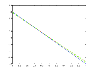
– : true function    -.-: first estimator $\quad\ldots$: truncated estimator
$n=10^{4}$ et $\Delta=10^{-1}$

Figure 2: Model 2: Double well and Laplace law

$$b(x)=-\left(x-1/4\right)^{3}-\left(x+1/4\right)^{3},\quad\sigma=\xi=1\textrm{ and Laplace law}$$

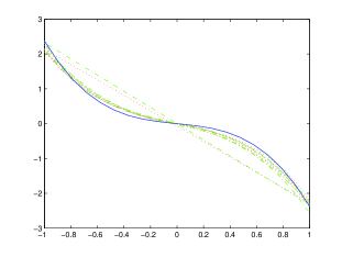
– : true function   -.-: first estimator$\qquad\ldots$: truncated estimator
$n=10^{4}$ et $\Delta=10^{-1}$

Figure 3: Model 3: Sine function

$$b(x)=-2x+\sin(3x),\;\sigma(x)=\xi(x)=\sqrt{(3+x^{2})/(1+x^{2})}\textrm{ jumps not sub-exponential }$$

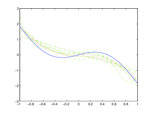
– : true function   -.-: first estimator$\quad\ldots$: truncated estimator
$n=10^{4}$ et $\Delta=10^{-1}$

Figure 4: Model 4: Lévy process

$$b(x)=-2x,\;\sigma(x)=\xi(x)=1\textrm{ jumps Lévy }$$

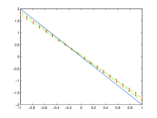
– : true function   -.-: first estimator$\quad\ldots$: truncated estimator
$n=10^{4}$ et $\Delta=10^{-1}$

Table 1: Model 1: Ornstein-Uhlenbeck and binomial law

$$b(x)=-2x,\;\sigma(x)=\xi(x)=1\>\textrm{and compound Poisson process (binomial law)}$$

		first estimator				truncated estimator
$n$	$\Delta$	$\hat{m}_{a}$	$\hat{r}_{a}$	$risk_{1}$	$or_{1}$	$\tilde{m}_{a}$	$\tilde{r}_{a}$	$risk_{2}$	$or_{2}$
$10^{3}$	$10^{-1}$	0	1.02	0.044	1.3	0	1.02	0.044	1.3
$10^{4}$	$10^{-1}$	0	1.02	0.011	1.3	0	1.02	0.011	1.3
$10^{3}$	$10^{-2}$	0	1.02	0.55	1.04	0	1.02	0.55	1.04
$10^{4}$	$10^{-2}$	0	1	0.047	1	0	1	0.047	1
$5.10^{4}$	$10^{-2}$	0.04	1	0.010	1.4	0	1	0.0053	1

$\hat{m}_{a}$, $\hat{r}_{a}$ and $\tilde{m}_{a}$, $\tilde{r}_{a}$ : average values of $\hat{m}$, $\hat{r}$ and $\tilde{m}$, $\tilde{r}$ on the 50 simulations.
$risk_{1}$ and $risk_{2}$ : means of the empirical errors of the adaptive estimators.

$or_{1}$ and $or_{2}$: means of $oracle=$empirical error of the adaptive estimator / empirical error of the best possible estimator.

Table 2: Model 2: Double well and Laplace law

$b(x)=-(x-1/4)^{3}-(x+1/4)^{3}$, $\sigma(x)=\xi(x)=1$ and Laplace law.

		first estimator				truncated estimator
$n$	$\Delta$	$\hat{m}_{a}$	$\hat{r}_{a}$	$risk_{1}$	$or_{1}$	$\tilde{m}_{a}$	$\tilde{r}_{a}$	$risk_{2}$	$or_{2}$
$10^{3}$	$10^{-1}$	0.02	1.0	0.12	3.1	0.02	1.0	0.12	3.1
$10^{4}$	$10^{-1}$	1.7	2.1	2e96	51	0.4	2.1	0.04	1.5
$10^{3}$	$10^{-2}$	0.26	1.2	1.8	3.1	0.06	1	0.51	1.4
$10^{4}$	$10^{-2}$	0.12	1.5	0.16	1.8	0.08	1.2	0.13	2.4
$5.10^{4}$	$10^{-2}$	0.30	2.5	0.035	1.6	0.26	2.5	0.019	1.8

$\hat{m}_{a}$, $\hat{r}_{a}$ and $\tilde{m}_{a}$, $\tilde{r}_{a}$ : average values of $\hat{m}$, $\hat{r}$ and $\tilde{m}$, $\tilde{r}$ on the 50 simulations.
$risk_{1}$ and $risk_{2}$ : means of the empirical errors of the adaptive estimators.

$or_{1}$ and $or_{2}$: means of $oracle=$empirical error of the adaptive estimator / empirical error of the best possible estimator.

Table 3: Model 3: Sine function and jumps not sub-exponential

$$b(x)=-2x+\sin(3x),\quad\sigma(x)=\xi(x)=\sqrt{(3+x^{2})/(1+x^{2})}\quad\textrm{and}\quad\nu(dz)\propto e^{-\sqrt{az}}/\sqrt{z}dz$$

		first estimator				truncated estimator
$n$	$\Delta$	$\hat{m}_{a}$	$\hat{r}_{a}$	$risk_{1}$	$or_{1}$	$\tilde{m}_{a}$	$\tilde{r}_{a}$	$risk_{2}$	$or_{2}$
$10^{3}$	$10^{-1}$	0.34	1.2	0.76	3.6	0.04	1.2	0.28	1.9
$10^{4}$	$10^{-1}$	0.8	2.2	0.082	1.3	0.68	2.2	0.073	1.2
$10^{3}$	$10^{-2}$	0.96	1.2	18	6.3	0.02	1.2	1.3	1.2
$10^{4}$	$10^{-2}$	0.78	1.4	1.5	4.3	0.12	1.4	0.24	3.3
$5.10^{4}$	$10^{-2}$	0.92	2.3	0.24	4.3	0.70	2.3	0.039	1.3

$\hat{m}_{a}$, $\hat{r}_{a}$ and $\tilde{m}_{a}$, $\tilde{r}_{a}$ : average values of $\hat{m}$, $\hat{r}$ and $\tilde{m}$, $\tilde{r}$ on the 50 simulations.
$risk_{1}$ and $risk_{2}$ : means of the empirical errors of the adaptive estimators.

$or_{1}$ and $or_{2}$: means of $oracle=$empirical error of the adaptive estimator / empirical error of the best possible estimator.

Table 4: Model 4: Lévy process

$$b(x)=-2x,\quad\sigma(x)=\xi(x)=1\quad\textrm{and}\quad\nu(dz)=\sum_{k=0}^{\infty}2^{k+2}(\delta_{2^{-k}}+\delta_{-2^{-k}})$$

		first estimator				truncated estimator
$n$	$\Delta$	$\hat{m}_{a}$	$\hat{r}_{a}$	$risk_{1}$	$or_{1}$	$\tilde{m}_{a}$	$\tilde{r}_{a}$	$risk_{2}$	$or_{2}$
$10^{3}$	$10^{-1}$	0.04	1.06	0.110	1.86	0.02	1.06	0.111	1.95
$10^{4}$	$10^{-1}$	0.06	1.06	0.0172	1.26	0.06	1.06	0.0176	1.22
$10^{3}$	$10^{-2}$	0.1	1.04	1.17	1.88	0	1.04	0.61	1.12
$10^{4}$	$10^{-2}$	0.04	1.08	0.11	1.25	0.02	1.08	0.068	1.25
$5.10^{4}$	$10^{-2}$	0.08	1.16	0.023	1.71	0	1.16	0.011	1.09

$\hat{m}_{a}$, $\hat{r}_{a}$ and $\tilde{m}_{a}$, $\tilde{r}_{a}$ : average values of $\hat{m}$, $\hat{r}$ and $\tilde{m}$, $\tilde{r}$ on the 50 simulations.
$risk_{1}$ and $risk_{2}$ : means of the empirical errors of the adaptive estimators.

$or_{1}$ and $or_{2}$: means of $oracle=$empirical error of the adaptive estimator / empirical error of the best possible estimator.

7 Auxiliary proofs

7.1 Decomposition on a lattice

Proposition 20.

If there exist some constants $c_{1}$, $c_{2}$ and $K$ independent of $D$, $n$, $\Delta$, $b$ and $\sigma$ and two constants $\alpha$ and $\beta$ independent of $n$ and $D$ such that, for any function $t\in S_{m}+S_{m}^{\prime}$:

$$\forall\eta,\zeta>0,\;\forall t\in S_{m}+S_{m^{\prime}}\;\left\|t\right\|_{\infty}\leq C\zeta,\;\mathbb{P}\left(f_{n}(t)\geq\eta,\left\|t\right\|_{n}^{2}\leq\zeta^{2}\right)\leq K\exp\left(-\frac{\eta^{2}n\beta}{\left(c_{1}\alpha^{2}\zeta^{2}+2Cc_{2}\alpha\eta\zeta\right)}\right),$$

then there exist some constants $C$ and $\kappa$ depending only of $\nu$ such that, if $D\leq n\beta$:

$$\mathbb{E}\left[\sup_{t\in\mathscr{B}_{m,m^{\prime}}}f_{n}^{2}(t)-\frac{\kappa\alpha^{2}D}{n\beta}\right]_{+}\leq CK\frac{\kappa\alpha^{2}D^{3/2}e^{-\sqrt{D}}}{n\beta}.$$

Let us consider an orthonormal (for the $L_{\varpi}^{2}$-norm) basis $\left(\psi_{\lambda}\right)_{\lambda\in\Lambda_{m,m^{\prime}}}$ of $S_{m,m^{\prime}}=S_{m}+S_{m^{\prime}}$ such that

$$\forall\lambda,\quad\textrm{card}\left(\left\{\lambda^{\prime},\;\left\|\psi_{\lambda}\psi_{\lambda^{\prime}}\right\|\neq 0\right\}\right)\leq\phi_{2}.$$

Let us set

$$\bar{r}_{m,m^{\prime}}=\frac{1}{\sqrt{D}}\sup_{\beta\neq 0}\frac{\left\|\sum_{\lambda}\beta_{\lambda}\psi_{\lambda}\right\|_{\infty}}{\left|\beta\right|_{\infty}}.$$

We obtain that

$$\left\|\sum_{\lambda}\beta_{\lambda}\psi_{\lambda}\right\|_{\infty}\leq\phi_{2}\left|\beta\right|_{\infty}\sup_{\lambda}\left\|\psi_{\lambda}\right\|_{\infty}\quad\textrm{et}\quad\left\|\psi_{\lambda}\right\|_{\infty}\leq\sqrt{D}\left\|\psi_{\lambda}\right\|_{L^{2}}\leq\pi_{1}\sqrt{D}\left\|\psi_{\lambda}\right\|_{\varpi}$$

then

$$\bar{r}_{m,m^{\prime}}\leq\bar{r}:=\phi_{2}\pi_{1}.$$

We need a lattice of which the infinite norm is bounded. We use Lemma 9 of Barron et al. (1999):

Result 21.

There exists a $\delta_{k}$-lattice $T_{k}$ of $L_{\varpi}^{2}\cap(S_{m}+S_{m^{\prime}})$ such that

$$\left|T_{k}\cap\mathscr{B}_{m,m^{\prime}}\right|\leq\left(5/\delta^{k}\right)^{D}$$

where $\delta_{k}=2^{-k}/5$ . Let us denote by $p_{k}(u)$ the orthogonal projection of $u$ on $T_{k}$. For any $u\in S_{m,m^{\prime}}$, $\left\|u-p_{k}(u)\right\|_{\pi}\leq\delta_{k}$ and

$$\sup_{u\in p_{k}^{-1}(t)}\left\|u-t\right\|_{\infty}\leq\bar{r}_{m,m^{\prime}}\delta_{k}\leq\bar{r}\delta_{k}.$$

Let us set $H_{k}=\ln(\left|T_{k}\cap\mathscr{B}_{m,m^{\prime}}\right|)$. We have that:

$$H_{k}\leq D\ln(5/\delta_{k})=D\left(k\ln(2)+\ln(5/\delta_{0})\right)\leq C(k+1)D.$$

The decomposition of $u_{k}$ on the $\delta_{k}$-lattice must be done very carefully: the norms $\left\|u_{k}-u_{k-1}\right\|_{\varpi}$ and $\left\|u_{k}-u_{k-1}\right\|_{\infty}$ must be controlled. Let us set

$$\mathscr{E}_{k}=\left\{u_{k}\in T_{k}\cap\mathscr{B}_{m,m^{\prime}},\quad\left\|u-u_{k}\right\|_{\varpi}\leq\delta_{k}\quad\textrm{et}\quad\left\|u-u_{k}\right\|_{\infty}\leq\bar{r}\delta_{k}\right\}.$$

We have that $\ln(\left|\mathscr{E}_{k}\right|)\leq H_{k}$. For any function $u\in\mathscr{B}_{m,m^{\prime}}$, there exist a series $(u_{k})_{k\geq 0}\in\prod_{k}\mathscr{E}_{k}$ such that

$$u=u_{0}+\sum_{k=1}^{\infty}\left(u_{k}-u_{k-1}\right).$$

Let us consider $(\eta_{k})_{k\geq 0}$ and $\eta\in\mathbb{R}$ such that $\eta_{0}+\sum_{k=1}^{\infty}\eta_{k}\leq\eta.$ We obtain:

$$\mathbb{P}\left(\sup_{u\in\mathscr{B}_{m,m^{\prime}}}\left|f_{n}(u)\right|>\eta\right) \leq \mathbb{P}\left(\exists\left(u_{k}\right)\in\prod\mathscr{E}_{k},\;\left|f_{n}(u_{0})+\sum_{k=1}^{\infty}f_{n}(u_{k}-u_{k-1})\right|>\eta_{0}+\sum_{k=1}^{\infty}\eta_{k}\right)$$ (16)

$$\leq P_{1}+\sum_{k=1}^{\infty}P_{2,k}$$

where

$$P_{1}=\sum_{u_{0}\in\mathscr{E}_{0}}\mathbb{P}\left(\left|f_{n}(u_{0})\right|>\eta_{0}\right)\quad\textrm{and}\quad P_{2,k}=\sum_{u_{k}\in\mathscr{E}_{k}}\mathbb{P}\left(\left|f_{n}(u_{k}-u_{k-1})\right|>\eta_{k}\right).$$

As $u_{0}\in T_{0}$, $\left\|u_{0}\right\|_{\varpi}\leq 1$ and $\left\|u_{0}\right\|_{\infty}\leq\bar{r}\sqrt{D}$. Moreover, $\left\|u_{0}\right\|_{n}^{2}\leq 3/2$$\left\|u_{0}\right\|_{\varpi}^{2}\leq 3\delta_{0}/2$. Then

$$\mathbb{P}\left(\left|f_{n}(u_{0})\right|>\eta_{0}\right)=\mathbb{P}\left(\left|f_{n}(u_{0})\right|>\eta_{0},\;\left\|u_{0}\right\|_{n}^{2}\leq 3\delta_{0}/2\right).$$

There exist two constants $c_{1}^{\prime}$ and $c_{2}^{\prime}$ depending only on $\delta_{0}$ and $\bar{r}$ such that

$$\mathbb{P}\left(\left|f_{n}(u_{0})\right|>\eta_{0}\right)\leq K\exp\left(-\frac{n\beta\eta_{0}^{2}}{c_{1}^{\prime}\alpha^{2}+2c_{2}^{\prime}\sqrt{D}\alpha\eta_{0}}\right).$$

Let us set $x_{0}$ such that $\eta_{0}=\alpha\left(\sqrt{c_{1}^{\prime}\left(x_{0}/\beta\right)}+c^{\prime}_{2}\sqrt{D}\left(x_{0}/\beta\right)\right)$. Then:

$$x_{0}\leq\frac{\beta\eta_{0}^{2}}{c_{1}^{\prime}\alpha^{2}+2c_{2}^{\prime}\sqrt{D}\alpha\eta_{0}}$$

and

$$\mathbb{P}\left(f_{n}(u_{0})>\eta_{0}\right)\leq K\exp\left(-nx_{0}\right).$$

Then

$$P_{1}\leq K\sum_{u_{0}\in\mathscr{E}_{0}}\exp\left(-nx_{0}\right)\leq K\exp\left(H_{0}-nx_{0}\right).$$ (17)

We have that

$$\left\|u_{k}-u_{k-1}\right\|_{\pi}^{2}\leq 2\left(\left\|u-u_{k-1}\right\|_{\pi}^{2}+\left\|u-u_{k}\right\|_{\pi}^{2}\right)\leq 5\delta_{k-1}^{2}/2$$

then $\left\|u_{k}-u_{k-1}\right\|_{n}^{2}\leq 15\delta_{k-1}^{2}/4$. As $u_{k-1},u_{k}\in\mathscr{E}_{k-1}\times\mathscr{E}_{k}$, it follows that $\left\|u_{k}-u_{k-1}\right\|_{\infty}^{2}\leq 5\delta_{k-1}^{2}\bar{r}^{2}/2$. There exists two constants $c_{3}$ and $c_{4}$ such that:

$$\mathbb{P}_{n}\left(\left|f_{n}(u_{k}-u_{k-1})\right|>\eta_{k}\right) = \mathbb{P}_{n}\left(\left|f_{n}(u_{k}-u_{k-1})\right|>\eta_{k},\;\left\|u_{k}-u_{k-1}\right\|_{n}^{2}\leq 15\delta_{k-1}^{2}/4\right)$$

$$\leq K\exp\left(-\frac{n\beta\eta_{k}^{2}}{c_{3}\alpha^{2}\delta_{k-1}^{2}+2c_{4}\alpha\delta_{k-1}}\right).$$

Let us fix $x_{k}$ such that $\eta_{k}=\delta_{k-1}a\left(\sqrt{c_{3}\left(x_{k}/\beta\right)}+c_{4}\left(x_{k}/\beta\right)\right)$. We obtain:

$$x_{k}\leq\frac{\beta\eta_{k}^{2}}{c_{3}\alpha^{2}\delta_{k-1}^{2}+2c_{4}\alpha\delta_{k-1}}$$

and

$$\mathbb{P}\left(\left|f_{n}(u_{k}-u_{k-1})\right|>\eta_{k}\right)\leq K\exp\left(-nx_{k}\right).$$

Then, $P_{2,k}\leq K\exp\left(H_{k-1}+H_{k}-nx_{k}\right)$ and

$$P_{2}=\sum_{k=1}^{\infty}P_{2,k}\leq K\sum_{k=1}^{\infty}\exp\left(H_{k-1}+H_{k}-nx_{k}\right).$$ (18)

Let us set $\tau>0$ and choose $(x_{k})$ (and then $(\eta_{k})$) such that

$$\begin{cases}\sqrt{D}nx_{0}=H_{0}+D+\tau\\ nx_{k}=H_{k-1}+H_{k}+(k+1)D+\tau.\end{cases}$$

Collecting the results, we obtain, by (16), (17) and (18):

$$\mathbb{P}\left(\sup_{u\in\mathscr{B}_{m,m^{\prime}}}\left|f_{n}(u)\right|>\eta\right)\leq C\left(e^{-D}e^{-\tau}+e^{-\sqrt{D}}e^{-\tau/\sqrt{D}}\right).$$ (19)

It remains to compute $\eta^{2}$. We denote by $C$ a constant depending only on $\delta_{0}$ and $\bar{r}$ . This constant may vary from one line to another. We have that:

$$\eta=\sum_{k=0}^{\infty}\eta_{k} \leq C\alpha\left(\sum_{k=1}^{\infty}\delta_{k-1}\left(\sqrt{\frac{x_{k}}{\beta}}+\frac{x_{k}}{\beta}\right)\right)+\alpha\left(\sqrt{\frac{x_{0}}{\beta}}+\sqrt{D}\frac{x_{0}}{\beta}\right).$$

Let us recall that $H_{k}=C(k+1)D$. Then, $nx_{k}=C(3k+2)D+\tau$ , $\sqrt{D}nx_{0}=CD+\tau$ and

$$\sum_{k=0}^{\infty}\frac{\delta_{k-1}x_{k}}{\beta}\leq\frac{1}{n\beta}\sum_{k=0}^{\infty}2^{-(k-1)}(C(3k+2)D+\tau)\leq C\frac{D+\tau}{n\beta}.$$

Moreover,

$$\sum_{k=0}^{\infty}\delta_{k-1}\sqrt{\frac{x_{k}}{\beta}}\leq C\frac{\sqrt{D}+\sqrt{\tau}}{\sqrt{n\beta}}.$$

As $D/n\beta\leq 1$, there exists a constant $\kappa$ such that

$$\eta^{2}\leq\kappa\alpha^{2}\left(\frac{D}{n\beta}+2\frac{\tau}{n\beta}+\frac{\tau^{2}}{n^{2}\beta^{2}}\right).$$

Then, according to (19):

$$\mathbb{P}\left(\sup_{u\in\mathscr{B}_{m,m^{\prime}}}f_{n}^{2}(u)>\kappa\alpha^{2}\left(\frac{D}{n\beta}+2\frac{\tau}{n\beta}+\frac{\tau^{2}}{n^{2}\beta^{2}}\right)\right)\leq C\left(e^{-D-\tau}+e^{-\sqrt{D}-\tau/\sqrt{D}}\right).$$ (20)

Furthermore

$$E := \mathbb{E}\left(\left[\sup_{u\in\mathscr{B}_{m,m^{\prime}}}f_{n}^{2}(u)-\kappa a^{2}\frac{D}{n\beta}\right]_{+}\right)$$

$$= \int_{0}^{\infty}\mathbb{P}\left(\sup_{u\in\mathscr{B}_{m,m^{\prime}}}f_{n}^{2}(u)>\kappa a^{2}\frac{D}{n\beta}+\tau\right)d\tau$$

Setting $\tau=\kappa\alpha^{2}\left(2y/n\beta+y^{2}/n^{2}\beta^{2}\right)$, it follows:

$$E=C\gamma^{2}\int_{0}^{\infty}\mathbb{P}\left(\sup_{u\in\mathscr{B}_{m,m^{\prime}}}f_{n}^{2}(u)>\kappa\alpha^{2}\left(\frac{D}{n\beta}+2\frac{y}{n\beta}+\frac{y^{2}}{n^{2}\beta^{2}}\right)\right)\left(\frac{2}{n\beta}+\frac{2y}{n^{2}\beta^{2}}\right)dy.$$

By (20),

$$E = C\kappa\alpha^{2}\left(e^{-D}+e^{-\sqrt{D}}\right)\left(\frac{1}{n\beta}\int_{0}^{\infty}ye^{-y/\sqrt{D}}dy\right)$$

$$\leq C\frac{\kappa\alpha^{2}}{n\beta}D^{3/2}e^{-\sqrt{D}}.$$

Acknowledgement:

the author wishes to thank M. Reiss and V. Genon-Catalot for helpful discussions.

References

- Applebaum (2004) Applebaum, D. (2004) Lévy processes and stochastic calculus, Cambridge Studies in Advanced Mathematics, volume 93. Cambridge University Press, Cambridge.
- Arlot and Massart (2009) Arlot, S. and Massart, P. (2009) Data-driven calibration of penalties for least-squares regression. Journal of Machine Learning Research, 10 pp. 245–279.
- Barron et al. (1999) Barron, A., Birgé, L. and Massart, P. (1999) Risk bounds for model selection via penalization. Probab. Theory Related Fields, 113 (3) pp. 301–413.
- Birgé and Massart (1998) Birgé, L. and Massart, P. (1998) Minimum contrast estimators on sieves: exponential bounds and rates of convergence. Bernoulli, 4 (3) pp. 329–375.
- Comte (2001) Comte, F. (2001) Adaptive estimation of the spectrum of a stationary gaussian sequence. Bernoulli, 7 (2) pp. 267–298.
- Comte et al. (2007) Comte, F., Genon-Catalot, V. and Rozenholc, Y. (2007) Penalized nonparametric mean square estimation of the coefficients of diffusion processes. Bernoulli, 13 (2) pp. 514–543.
- Dellacherie and Meyer (1980) Dellacherie, C. and Meyer, P.A. (1980) Probabilités et potentiel. Chapitres V à VIII, Actualités Scientifiques et Industrielles [Current Scientific and Industrial Topics], volume 1385. Hermann, Paris, revised edition. Théorie des martingales. [Martingale theory].
- DeVore and Lorentz (1993) DeVore, R.A. and Lorentz, G.G. (1993) Constructive approximation, Grundlehren der Mathematischen Wissenschaften [Fundamental Principles of Mathematical Sciences], volume 303. Springer-Verlag, Berlin.
- Gobet et al. (2004) Gobet, E., Hoffmann, M. and Reiß, M. (2004) Nonparametric estimation of scalar diffusions based on low frequency data. Ann. Statist., 32 (5) pp. 2223–2253.
- Hoffmann (1999) Hoffmann, M. (1999) Adaptive estimation in diffusion processes. Stochastic Process. Appl., 79 (1) pp. 135–163.
- Ishikawa and Kunita (2006) Ishikawa, Y. and Kunita, H. (2006) Malliavin calculus on the Wiener-Poisson space and its application to canonical SDE with jumps. Stochastic Process. Appl., 116 (12) pp. 1743–1769.
- Liptser and Shiryaev (2001) Liptser, R.S. and Shiryaev, A.N. (2001) Statistics of random processes. I, Applications of Mathematics (New York), volume 5. Springer-Verlag, Berlin, expanded edition. General theory, Translated from the 1974 Russian original by A. B. Aries, Stochastic Modelling and Applied Probability.
- Mai (2012) Mai, H. (2012) Efficient maximum likelihood estimation for lévy-driven ornstein-uhlenbeck processes.
- Mancini and Renò (2011) Mancini, C. and Renò, R. (2011) Threshold estimation of Markov models with jumps and interest rate modeling. J. Econometrics, 160 (1) pp. 77–92.
- Masuda (2007) Masuda, H. (2007) Ergodicity and exponential -mixing bounds for multidimensional diffusions with jumps. Stochastic Process. Appl., 117 (1) pp. 35–56.
- Meyer (1990) Meyer, Y. (1990) Ondelettes et opérateurs. I. Actualités Mathématiques. [Current Mathematical Topics]. Hermann, Paris. Ondelettes. [Wavelets].
- Rubenthaler (2010) Rubenthaler, S. (2010) Probabilités : aspects théoriques et applications en filtrage non linéaire, systèmes de particules et processus stochastiques.. Habilitation à diriger des recherches, Université de Nice-Sophia Antipolis, France.
- Schmisser (2010) Schmisser, E. (2010) Estimation non paramétrique pour des processus de diffusion. Ph.D. thesis, Université Paris Descartes.
- Schmisser (2013) Schmisser, E. (2013) Penalized nonparametric drift estimation for a multidimensional diffusion process. Statistics, 47 (1) pp. 61–84. URL http://dx.doi.org/10.1080/02331888.2011.591931.
- Shimizu (2008) Shimizu, Y. (2008) Some remarks on estimation of diffusion coefficients for jump-diffusions from finite samples. Bull. Inform. Cybernet., 40 pp. 51–60.
- Shimizu and Yoshida (2006) Shimizu, Y. and Yoshida, N. (2006) Estimation of parameters for diffusion processes with jumps from discrete observations. Stat. Inference Stoch. Process., 9 (3) pp. 227–277.