A spectroscopic survey of Andromeda’s Western Shelf

Abstract

The Andromeda galaxy (M31) shows many tidal features in its halo, including the Giant Southern Stream (GSS) and a sharp ledge in surface density on its western side (the W Shelf). Using DEIMOS on the Keck telescope, we obtain radial velocities of M31’s giant stars along its NW minor axis, in a radial range covering the W Shelf and extending beyond its edge. In the space of velocity versus radius, the sample shows the wedge pattern expected from a radial shell, which is detected clearly here for the first time. This confirms predictions from an earlier model of formation of the GSS, which proposed that the W Shelf is a shell from the third orbital wrap of the same tidal debris stream that produces the GSS, with the main body of the progenitor lying in the second wrap. We calculate the distortions in the shelf wedge pattern expected from its outward expansion and angular momentum, and show that these effects are echoed in the data. In addition, a hot, relatively smooth spheroid population is clearly present. We construct a bulge-disk-halo $N$-body model that agrees with surface brightness and kinematic constraints, and combine it with a simulation of the GSS. From the contrasting kinematic signatures of the hot spheroid and shelf components, we decompose the observed stellar metallicity distribution into contributions from each component using a non-parametric mixture model. The shelf component’s metallicity distribution matches previous observations of the GSS superbly, further strengthening the evidence they are connected and bolstering the case for a massive progenitor of this stream.

1 INTRODUCTION

The Andromeda galaxy (M31) lies close enough for us to resolve its individual stars, at a position relatively unobscured by the Milky Way (MW) disk. Thus it represents perhaps our best opportunity to examine the complete structure of a large spiral galaxy in great detail. The region that we might term M31’s inner halo or outer disk appears quite irregular in resolved-star maps (Ibata et al., 2001; Ferguson et al., 2002; Irwin et al., 2005; Ibata et al., 2007; McConnachie et al., 2009; Tanaka et al., 2010). These maps show numerous substructures, some of which have been catalogued and named, although stars are distributed continuously throughout M31’s halo out to at least 150 kpc.

Pencil-beam spectroscopy and photometry brings some order to this complicated scene. Ibata et al. (2005) argues much of the structure is an outer extension of M31’s disk, with a clumpy structure and hot or thick disk kinematics. It also seems much of the structure is due to M31’s giant southern stream or GSS (Ibata et al., 2001). Ferguson et al. (2002) first suggested a connection between the GSS and the “NE Shelf” feature extending from the NE side of the M31 disk (see Fig. 1), which appears to have a red population of red giant branch (RGB) stars and thus is inferred to be metal-rich. Fardal et al. (2007, hereafter F07) pointed out a similar shelf on the western side of M31 (W Shelf), which they inferred to be a third wrap of the stream using an $N$-body simulation of the stream’s formation. Gilbert et al. (2007) found a structure through RGB star kinematics on the southeast minor axis (the “SE Shelf”) and identified it as the fourth wrap of this stream. Indeed, Richardson et al. (2008) found most of the dense structures in the inner halo examined by their deep Hubble Space Telescope (HST) observations could be classified as either “disk-like” or “stream-like”, with the positions of the “stream-like” fields matching well to the F07 model.

These two components cannot be the whole story, however. Spectroscopy also offers evidence of a smoother hot halo component (Guhathakurta et al., 2005, 2006; Chapman et al., 2006; Kalirai et al., 2006a; Gilbert et al., 2007). There appears to be an upward break in the surface brightness profile around 20–$30\,\mbox{kpc}$ (Irwin et al., 2005; Guhathakurta et al., 2005; Ibata et al., 2007) and a decrease in the metallicity in about the same place (Kalirai et al., 2006a; Koch et al., 2008). It is much disputed whether the “inner halo” region from 10–$20\,\mbox{kpc}$ is dominated by a halo component (Pritchet & van den Bergh, 1994; Durrell et al., 2001) the bulge (Guhathakurta et al., 2005; Kalirai et al., 2006a), the disk (Ibata et al., 2007; Courteau et al., 2011), or by a mix of these plus cold substructures (Gilbert et al., 2007). Other kinematic anomalies such as the “second stream” detected by Kalirai et al. (2006b) and Gilbert et al. (2009) currently lack an explanation. One might also expect tidal features from M32 or NGC 205 (M110), due to their location near M31’s center and distorted isophotes (Choi et al., 2002).

To better understand this complex structure, it is important to deduce how many components there are and determine for each its distribution in space, velocity, stellar age, and metallicity. A key ingredient in this will be a firm determination of the orbit of the GSS and the spatial coverage of its debris. The F07 model matches many features of the morphology and kinematics, but it is not the only suggestion for the orbit of the stream (Ibata et al., 2001; Merrett et al., 2003; Fardal et al., 2006; Hammer et al., 2010). A crucial test of the model comes in the W shelf region. The shelf stars are expected to exhibit a distinctive kinematic pattern in this model. F07 presented some kinematic evidence for this model from planetary nebulae and RGB stars, but this was more suggestive than conclusive.

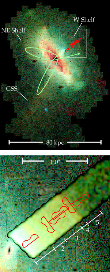
Figure 1: Top: star-count map from the INT survey of M31 (Irwin et al., 2005, image created by M. Irwin), with our Keck/DEIMOS spectroscopic multislit masks indicated in red. Blue, green, and red channels indicate the density of stars in separate color ranges on the RGB. The red channel contains the reddest, most metal-rich RGB stars. M31’s disk is apparent in red, and the main tidal features discussed in the text are indicated by labels. The W Shelf in particular is just visible as a faint but sharp edge to the NW of M31. The box shows the area covered in the bottom panel. The looping arrow indicates the progenitor’s path in our model. Bottom: enlargement of the region around our spectroscopic masks. Here a matched-filter map from the Subaru/SuprimeCam imaging survey (Tanaka et al., 2010) is overlaid, forming a diagonal stripe from lower left to upper right. The radial zones 1–5 used later are indicated.

In this paper we present new spectroscopy of the resolved stellar population in the W Shelf region that shows clear evidence for distinct shelf and hot spheroid components. This kinematic data agrees very well with the prediction from an updated version of the F07 model, which was run before the observations were reduced. §2 provides details on the observations and our $N$-body model. §3 analyzes the observations, first showing (§3.1) the distributions of the stars in position, velocity, and metallicity space. We then use the $N$-body model (§3.2) to separate the shelf and hot halo components in the observations, and thereby infer their distinct metallicity distributions. §4 concludes the paper by connecting our results to previous results on M31’s GSS and other inner halo populations, and placing our results in the broader context of halo structure in other galaxies. An Appendix provides a discussion of shell kinematics, including a formula for the velocity envelope in the generically correct case of an expanding shell.

2 METHODS

2.1 Observational data

Table 1: Spectroscopic observations

	Radial	Radius	Pointing center:		PA	Observation	Exposure	Seeing	Science	Confirmed	M31
Mask	Zone	(kpc)	$\alpha_{\rm J2000}$	$\delta_{\rm J2000}$	(∘)	Date (UT)	Time (s)	(”)	Targetsa	Starsb	Starsc
NW1V_1	1	13.1	0:38:36.33	41:50:11.8	$127$	2009 Aug 22	3600	0.5–0.8	279	56	46
NW1dV	2	18.1	0:37:07.94	42:05:35.8	$-143$	2009 Aug 21	3600	0.6–0.7	213	102	78
NW2V_1	3	20.6	0:36:20.72	42:12:08.5	$-53$	2009 Aug 21	3000	0.5–0.6	213	89	62
NW2V_2	3	21.6	0:36:07.90	42:15:48.4	$127$	2009 Aug 21	3000	0.5–0.7	208	100	62
NW2dV	4	24.2	0:35:18.87	42:23:22.8	$-143$	2009 Aug 22	3300	0.5–0.6	201	124	90
NW3V_1	5	26.8	0:34:22.67	42:28:13.8	$-53$	2009 Aug 21	3000	0.5	193	76	25

^aTotal number of slits on the mask.

^bObjects with secure radial velocities identified as either MW dwarfs or M31 giants.

^cObjects with secure radial velocities identified as M31 giants.

The data in this paper was obtained as part of the Spectroscopic and Photometric Landscape of Andromeda’s Stellar Halo (SPLASH) survey. Our spectroscopic survey area is embedded within the imaging survey of Tanaka et al. (2010), conducted with Suprime-Cam on the Subaru Telescope. That survey had the goal of quantifying the surface brightness profile and metallicity of the M31 halo and detecting streams and other substructure, by means of deep color-magnitude diagrams (CMDs) obtained mostly along the SE and NW minor axes of M31. The SE minor axis had earlier been studied intensively by means of wide-field photometry of individual stars, extremely deep CMDs obtained with HST, and resolved-star spectroscopy (Pritchet & van den Bergh, 1994; Durrell et al., 2001; Brown et al., 2003; Irwin et al., 2005; Brown et al., 2006, 2007, 2008; Ibata et al., 2007; Gilbert et al., 2007). In part because of increasing MW foreground to the north, the NW minor axis had received much less attention. Along the NW minor axis, the Subaru survey consists of a series of partially overlapping images that form a continuous stripe in the range $11\,\mbox{kpc}\la R\la 104\,\mbox{kpc}$. The survey used $V$ and $I$ filters on the Johnson-Cousins Vega-based magnitude system and probed down to 50% completeness limits of $V=25.7$, $I=24.9$.

Our spectroscopic survey leverages the earlier imaging survey to obtain kinematics of M31’s inner spheroid region, in particular covering the W Shelf feature that is prominent in Fig. 1. The blue, green, and red channels of the Subaru map are constructed from explicit cuts in metallicity with boundaries in $[\mathrm{Fe}/\mathrm{H}]$ of $-2.31$, $-1.71$, $-0.71$, and $0.0$, and due to their different input data and construction do not match the larger-scale Isaac Newton Telescope (INT) map exactly. Nevertheless, both maps show the W Shelf clearly as a red, metal-rich feature with a sharp edge, which is more easily seen in the narrow Subaru portion in the lower panel. The observation pattern of the Subaru survey involved small regions where adjacent Suprime-Cam pointings fields overlapped, and the resulting source catalog is broken up into regions with either single or double coverage. We orient the DEIMOS masks parallel to M31’s minor axis, except within the overlap regions, where we orient the masks perpendicular to the minor axis to fit inside the double coverage area. The six spectroscopic masks are described in Table 1 and shown in Fig. 1. Because two of the masks nearly overlap, these six masks result in five separated radial “zones”, labeled 1–5 from innermost to outermost in the discussion below. Comparing to the maps from the INT and Subaru imaging surveys shown in Fig. 1, we can see that zones 1–4 lie within the boundary of the W Shelf feature and zone 5 just outside of it.

The spectroscopic targets were chosen from the catalog of sources obtained from the Subaru survey of M31 (Tanaka et al., 2010). This catalog was produced using PSF-fitting photometry using DAOPHOT-II. Extended objects (mostly galaxies, as well as some blended stars) were removed from the target sample based on a set of DAOPHOT-II morphological parameters. Details of this procedure are in Tanaka et al. (2010).

At these relatively high surface brightness levels in Andromeda’s halo, we expect from previous experience that most of the stellar targets are M31 stars, at least below the tip of the RGB at M31’s distance at $I=20.5$. For simplicity, then, our target selection uses only the $I$ magnitude, which roughly measures the flux in the wavelength range of our spectra. We choose targets in the range $20.5<I<23.0$. We assign a priority to each target which decreases linearly with magnitude by a factor of two over this range. Our mask design software then chooses a slit pattern with the aim of maximizing the sum of priorities over the mask using a minimum slit length criterion. This produces a bias toward selection of the brighter stars, though stars are selected in significant numbers within the entire magnitude range specified.

Observations were obtained with DEIMOS at the Keck II telescope in the fall of 2009 in good seeing conditions. The observational setup was similar to that in Gilbert et al. (2007). We observed 3 sub-exposures for each of the six masks, with a total observing time of 45 to 60 minutes. Details of the observations are listed in Table 1. We used the DEIMOS spectrograph with a $1200\,\mbox{mm}^{-1}$ grating. The central wavelength was 7800 Å, with a range of about 6450–9150 Å (depending somewhat on the slit location on the mask). The dispersion was 0.33 Å $\mbox{pixel}^{-1}$, and the spectral resolution about 1.3 Å FWHM.

The spectra were reduced and analyzed using a modified version of the SPEC2D and SPEC1D software developed by the DEEP2 team at the University of California, Berkeley. These routines perform standard spectral reduction steps, including flat-fielding, night-sky emission line removal, and extraction of one-dimensional spectra from the two-dimensional spectra. Reduced one-dimensional spectra were cross-correlated with a library of template stellar spectra to determine the radial velocity of the object. Each spectrum was visually inspected and assigned a quality code based on the number and quality of absorption lines. Spectra with at least two spectral features (even if one of them is marginal) were considered to have secure velocity measurements. The position of the atmospheric A-band in the observed spectrum was used to correct the observed velocity for imperfect centering of the star in the slit (Simon & Geha, 2007; Sohn et al., 2007). A heliocentric correction was applied to the measured velocities based on the sky position of each mask and the date and time of the observation. More details of these procedures are provided in earlier papers, including Guhathakurta et al. (2006) and Gilbert et al. (2007).

On several of the masks, a significant fraction of the slits failed to yield acceptable spectra. Most of these failures were localized by position, so that broad swaths of the mask area are missing any velocity measurements. These failures were caused by temporary problems with the CCD readout electronics and possible problems with the calibration data. We are confident that the rate of such failures has no intrinsic dependence on velocity, and thus introduces no bias into our kinematic analysis below.

The median velocity error for the stars presented in this paper is $3\,\mbox{km}\,\mbox{s}^{-1}$, and the maximum is $13\,\mbox{km}\,\mbox{s}^{-1}$. Errors are estimated from the cross-correlation profile, including a modest scaling factor that is empirically calibrated by previous duplicate measurements of individual stars on overlapping DEIMOS masks. We ignore these small velocity errors in the analysis below, as the intrinsic widths of the velocity distributions we are interested in are much larger.

For our metallicity estimates we use photometric rather than spectroscopic methods, since for our combination of deep photometry and moderate $S/N$ spectroscopy we judge the former to be more reliable. We estimate metallicities from the $V$ and $I$ magnitudes using the procedure described in Gilbert et al. (2007) (rather than that in Tanaka et al., 2010), for consistency with the dwarf-giant separation algorithm. The $[\mathrm{Fe}/\mathrm{H}]$ values are based on a comparison of the star’s position within the CMD to a finely spaced grid of theoretical 12 Gyr, [$\alpha$/Fe] $=0$ stellar isochrones (Kalirai et al., 2006a; VandenBerg et al., 2006) adjusted to the distance of M31. Metallicities of the MW stars as assigned by this algorithm are therefore not meaningful.

We classify the stars in the sample using the likelihood method of Gilbert et al. (2006). We use the following criteria:

• The measured equivalent width of the Na I doublet at 8190 Å combined with the $V-I$ color of the star.

• The strength of the Ca II triplet absorption lines, as measured by comparison of the star’s photometric (CMD-based) vs. spectroscopic (Ca triplet-based) metallicity estimates.

• The position of the star in an $(V,I)$ CMD with respect to theoretical RGB isochrones.

• The radial velocity of the star.

Gilbert et al. showed that this combination of diagnostics can yield a reasonably reliable separation of MW from M31 stars. The method of Gilbert et al. (2006) can also incorporate additional criteria such as photometry in the surface-gravity-sensitive DDO51 band, but this was not available for our sample. We flag stars with a M31 membership probability of greater than 50% and CMD locations reasonably close to the RGB as M31 stars (classes 1–3 in the terminology of Gilbert et al. 2006). The membership probability is quite bimodal, and over the sample of identified M31 stars, the mean membership probability is 94%. A few misclassifications are inevitable, particularly in the higher-velocity part of the sample ($v\sim-100\,\mbox{km}\,\mbox{s}^{-1}$) where the M31 and MW velocity distributions overlap (see Gilbert et al., 2007 for a full discussion). Our final sample contains 547 stars, of which 363 are flagged as M31 giants and 184 as MW dwarfs.

2.2 Simulation

The $N$-body simulation we use in this paper is a slightly updated version of the simulation in F07. From our ongoing work with automated fitting of the GSS (Fardal et al., in preparation), we selected a set of parameters that offered good agreement with a set of observational constraints. The orbital initial conditions in the sky coordinate system (see Fardal et al., 2006) are $x=-24.0\,\mbox{kpc}$, $y=0.09\,\mbox{kpc}$, $z=44.1\,\mbox{kpc}$, $v_{x}=29.1\,\mbox{km}\,\mbox{s}^{-1}$, $v_{y}=8.7\,\mbox{km}\,\mbox{s}^{-1}$, $v_{z}=-77.6\,\mbox{km}\,\mbox{s}^{-1}$, and the model was run for $0.972\,\mbox{Gyr}$ to reach its present point. The input satellite is a Plummer model with mass $M_{s}=3.09\times 10^{9}\,M_{\sun}$ and scale length $r_{s}=1.16\,\mbox{kpc}$, created with the ZENO library. We take the mass to be purely stellar here. We reason that much of the dark halo mass will have been stripped off in earlier pericentric passages, as is typically found in cosmological simulations (Libeskind et al., 2011) and analytic models (Watson et al., 2012) of satellite accretion. The initial mass indicates a relatively massive galaxy rather than a dark-matter-dominated dwarf. Mori & Rich (2008) have considered a GSS progenitor with a massive halo, finding that a total satellite mass of $\la 5\times 10^{9}\,M_{\sun}$ is required to avoid perturbing M31’s disk too much. (The effects of dark matter in the progenitor will be considered in more depth in Fardal et al., in preparation, where we find that the moderate amounts of dark matter allowed by various constraints do not radically change the nature of the simulations.)

The progenitor initially follows the trajectory shown in Fig. 1 (which assumes a test-particle orbit), and though its tidal debris is significantly extended it generally follows a similar trajectory. This makes the GSS the first wrap of the orbit since the initial pericenter, the NE shelf the second, and the W Shelf the third. The W Shelf grows outwards over the last 300–400 Myr from M31’s center to its current size. For convenience we refer throughout to all the particles from this simulation as “GSS” material, except when explicitly distinguishing different radial wraps.

We base our fixed gravitational potential model on Geehan et al. (2006). We use a Hernquist bulge with $r_{b}=0.61\,\mbox{kpc}$ and $M_{b}=3.39\times 10^{10}\,M_{\sun}$, a Miyamoto-Nagai disk (replacing our earlier exponential disk for computational speed) with $a_{d}=5.94\,\mbox{kpc}$, $b_{d}=0.4\,\mbox{kpc}$, and $M_{d}=8.07\times 10^{10}\,M_{\sun}\,\mbox{kpc}^{-2}$, and a Navarro-Frenk-White (NFW) halo (Navarro et al., 1996) with $r_{h}=24.2\,\mbox{kpc}$, $\rho_{h}\equiv\delta_{c}\rho_{c}=5.85\times 10^{6}\,M_{\sun}\,\mbox{kpc}^{-3}$, and $M(r<r_{h})=2.02\times 10^{11}\,M_{\sun}$. Our model is qualitatively quite similar to that in F07, but better fits the velocity in the GSS itself and the radii of the NE and W shelves. The run was conducted with the code PKDGRAV, in advance of the observational reductions.

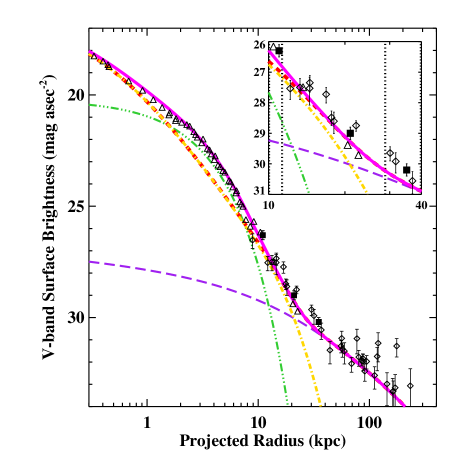
Figure 2: $V$-band surface brightness distribution of our model, compared to data. Solid magenta: total model surface brightess. Dot-dashed yellow: bulge. Triple-dot-dashed green: disk. Long-dashed purple: halo. Dashed red: bulge and halo combined (or “spheroid”). Solid squares: Brown et al. (2003, 2007, 2008) photometric fields. Open triangles: Pritchet & van den Bergh (1994) photometric fields. Open diamonds: Gilbert et al. (in preparation) spectroscopic fields. All except the Gilbert points are taken from the minor axis. The inset expands the region studied in this paper; dashed vertical lines show the complete radial range of the target stars.

We supplement this GSS simulation with an $N$-body realization of M31 itself. We draw parameters for the bulge from the model just listed. However, for better agreement with the outer surface brightness profile of M31, we truncate the bulge density starting at $11\,\mbox{kpc}$ using the default ZENO truncation scheme, which assumes continuous values and slopes at the truncation point and thereafter adopts a form $\rho(r)\propto r^{-2}\exp(-r/r_{\ast})$. For the disk we use a true exponential disk as in the Geehan et al. (2006) model, with $M_{d}=7.34\times 10^{10}\,M_{\sun}\,\mbox{kpc}^{-2}$ and $r_{d}=5.4\,\mbox{kpc}$, which is similar to the Miyamoto disk used in the simulation in terms of its dynamical effects. We add a stellar halo component not present in the Geehan et al. (2006) model, postulating that it follows the dark halo component and thus has $r_{h}=24.2\,\mbox{kpc}$. The mass is normalized to match surface brightness measurements and kinematic samples as described below. We set the characteristic density $\rho_{0}=\delta_{c}\rho_{c}=1.30\times 10^{4}\,M_{\sun}\,\mbox{kpc}^{-3}$, or $M(r<r_{h})=4.50\times 10^{8}\,M_{\sun}$. As with the input satellite, ZENO generates the spheroid component particle velocities from the full distribution function generated by inversion of an Abel integral, to ensure equilibrium with the potential of the baryonic components and dark halo. Although we do not evolve the $N$-body snapshot, from previous test simulations we know it is very close to equilibrium.

For the combined model, the virial radius (here defined as the radius where the mean enclosed density is 200 times the critical density, assuming $H_{0}=71\,\mbox{km}\,\mbox{s}^{-1}\,\mbox{Mpc}^{-1}$) is $r_{200}=242\,\mbox{kpc}$ and the corresponding virial mass is $M_{200}=1.66\times 10^{12}\,M_{\sun}$. (For a virial threshold of 100, these quantities would be $319\,\mbox{kpc}$ and $1.91\times 10^{12}\,M_{\sun}$ respectively.) The mass within $125\,\mbox{kpc}$, sometimes used as a benchmark of M31’s halo mass, is $1.13\times 10^{12}\,M_{\sun}$. The mass of the stellar halo component within $r_{200}$ is $1.2\times 10^{9}\,M_{\sun}$, more than a factor of ten lower than the bulge mass.

The surface brightness distribution produced by these components is shown in Fig. 2. Here we assume observed (not dust-corrected) $M/L_{V}$ values of 5.6 for the bulge and 5.0 for the disk, based on estimates of their $M/L_{R}$ and $V-R$ color in Geehan et al. (2006). For the halo we assume a lower $M/L_{V}=2.5$, which is reasonable for old stellar isochrones of the low metallicity ($[\mathrm{Fe}/\mathrm{H}]<-1.0$) thought to be prevalent in the halo (Kalirai et al., 2006a; Koch et al., 2008). The smaller $M/L_{V}$ of the halo compared to the bulge is justifiable based on the lower metallicity and extinction in the halo. Of course, these $M/L_{V}$ values are fairly uncertain, and adopting a single $M/L_{V}$ for each component is itself a gross oversimplification.

There have been many observational studies of M31’s surface brightness, most of which have concentrated on the SE minor axis. We include three datasets here: the photometric survey of Pritchet and van den Bergh (Pritchet & van den Bergh, 1994), the spectroscopic survey of Gilbert et al. (in preparation), and three points from deep HST surveys Brown et al. (2003, 2007, 2008). The Gilbert et al. values are calculated after removal of obvious substructure, and have been normalized to the surface brightness in the HST deep fields. The HST values in turn were calculated by summing the individual stellar luminosities using data products in Brown et al., 2009. This method should be more accurate because the HST fields probe nearly the entire luminosity function, because they require no uncertain sky subtraction, and because they directly overlap several of the spectroscopic fields. We calculate the normalization using three spectroscopic fields that overlap the HST fields, making a small correction for the slight differences in mean radii between corresponding HST and spectroscopic fields. We choose the normalization value using a minimum $\chi^{2}$ criterion, with results shown on the plot. It can be seen that the total surface brightness in our model traces observational data reasonably well, in particular reproducing the previously known upward kink around 20–30 kpc (Irwin et al., 2005; Courteau et al., 2011). Although some discrepancies may be present, these are no larger than the scatter in the observational points. Some of the observations are still likely contaminated with substructure in the outer parts of the halo, so our model is chosen to follow the lower envelope of the data.

Both bulge and halo components are represented here by spherical, isotropic populations. We regard the distinction between these hot bulge and halo components as somewhat artificial. The evidence for two components in the surface brightness data is merely the previously mentioned upward kink, and the separation between bulge and halo in our model is undoubtedly influenced by our choice of radial profiles. Thus we prefer to discuss them collectively as the “spheroid” component, which is shown by the dashed red line in Fig. 2. The transition between the surface mass density of these two components occurs at 25 kpc, and that in the $V$ light at 21 kpc. We note the decomposition here is rather different than that for the $I$-band decomposition in Courteau et al. (2011), in which the bulge-halo transition occurs at a mere 3 kpc, due largely to differences in the assumed radial profiles. Courteau’s preferred model uses a de Vaucouleurs bulge and a cored power-law halo, and these have very different dependences at small and large radii than our functional forms. The total spheroid components in our model and in the preferred model of Courteau et al. (2011) are not so different, however. Even with a crude correction for $V-I$ color, we find the two profiles differ usually by less than 0.3 magnitudes within the virial radius and never by as much as a magnitude. The two largest discrepancies come at the bulge-halo transition points in the two models, and lie either in the region where the disk dominates the spheroid, or in the halo region where the statistical and systematic uncertainties are high.

The spheroid star velocity dispersion at 30 kpc in our model is $118\,\mbox{km}\,\mbox{s}^{-1}$ and very close to Gaussian. From measurements elsewhere in M31’s halo, we expect a nearly Gaussian distribution with a mean of zero and dispersion of about $130\,\mbox{km}\,\mbox{s}^{-1}$ in the hot spheroid (Chapman et al., 2006; Gilbert et al., 2007), suggesting the model spheroid component is reasonable.

We use equal particle masses for all components of our simulation, so that the number density of simulation particles is proportional to the mass density within the model. In principle the ratio of mass density to the number of RGB stars that are selected in the observations is dependent on stellar population. However, the bulge and halo population at these radii have relatively old stellar populations lacking in stars with $<5\,\mbox{Gyr}$ (Brown et al., 2003, 2006, 2007), so their RGB density per unit mass should not be too different from the stream material. As we will see later, the disk component plays at most a small role just in the innermost mask, so the possible large difference in its stellar population is not of great concern. Furthermore, accurate predictions of the kinematic component normalizations are never required by our analysis methods below. Rather, we allow freedom in fitting the normalizations of the different components, and instead use their spatial and velocity distributions as a template to set the observed relative strength of the component contributions.

When comparing to the observations, we enhance our particle statistics by using a larger area than is covered by the observed masks. We choose particles within the region with major axis position $|X|<0.3^{\circ}$, slightly wider than any of our masks, as well as minor axis position $0.7^{\circ}<Y<2.2^{\circ}$. In this we rely on the fact that over small scales in the simulation the velocity distributions change slowly with position, and depend mainly on projected radius.

3 ANALYSIS AND RESULTS

3.1 Observed distributions

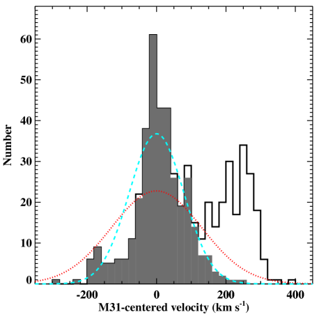
Figure 3: Histogram of the stellar velocities in our sample. The solid histogram shows only those stars classified as M31 giant stars, while the open histogram includes the contribution from foreground dwarfs. The dotted line shows the best Gaussian fit to the M31 stars assuming the expected spheroid velocity dispersion of $130\,\mbox{km}\,\mbox{s}^{-1}$, while the dashed line shows the best fit with velocity dispersion left free. Neither distribution adequately fits the data.

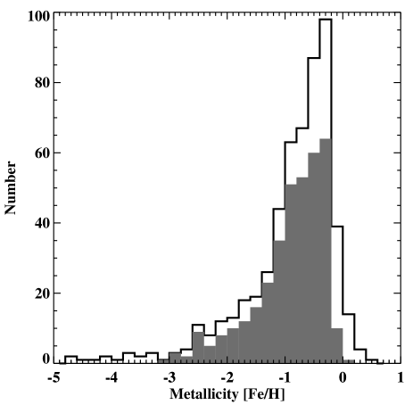
Figure 4: Histogram of the stellar metallicities in our sample, with the solid histogram showing only the M31 giant stars. We use photometric metallicities throughout, since we believe these to be more reliable than spectroscopic metallicities at the noise level of our spectra.

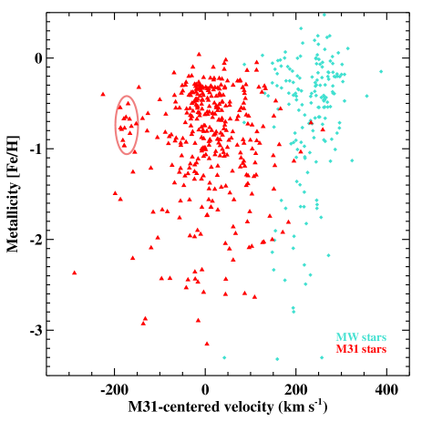
Figure 5: Metallicity versus velocity for individual stars in our sample. Triangles denote M31 giant stars, and diamonds denote MW dwarf stars. (Assigned metallicities of the MW stars are not meaningful as explained in the text.) We have placed an ellipse around the small clump at $v\approx-175\,\mbox{km}\,\mbox{s}^{-1}$, $\mbox{[Fe/H]}\approx-0.75$.

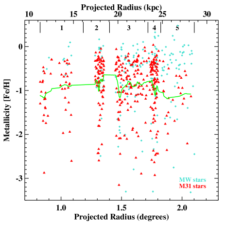
Figure 6: Metallicity versus radius for individual stars in our sample, with symbols the same as Fig. 5. The green line shows the metallicity boxcar smoothed over radial rank order. The numbers and separators near the top indicate the radial zones.

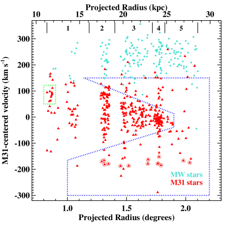
Figure 7: Velocity versus radius for individual stars in our sample. Red triangles denote M31 giant stars, and cyan diamonds denote MW dwarf stars. The stars within the ellipse in Fig. 5 are circled. The green box indicates a clump of stars possibly associated with NGC 205. The blue polygon shows the test region used to calculate the velocity dispersion of the hot component.

In Fig. 3, we show the overall radial velocity distribution of the observed stars. Throughout, we state velocity relative to M31’s systemic velocity of $-300\pm 4\,\mbox{km}\,\mbox{s}^{-1}$ (de Vaucouleurs et al., 1991). We split the distribution into M31 and MW stars. As discussed in § 2, we expect a mean of zero and dispersion of $\sim\!130\,\mbox{km}\,\mbox{s}^{-1}$ if the distribution is dominated by the hot spheroid. Neither this distribution, nor the best Gaussian fit with dispersion left free, fits the distribution at all well, as can be seen in the figure and as verified by $\chi^{2}$ tests. Most stars are contained within $|v|<50\,\mbox{km}\,\mbox{s}^{-1}$, but a large fraction inhabit much broader tails of the distribution. In contrast, a fit with dispersion $130\,\mbox{km}\,\mbox{s}^{-1}$ to only the values with $|v|>100\,\mbox{km}\,\mbox{s}^{-1}$ is statistically acceptable. The apparent peaks near $-175\,\mbox{km}\,\mbox{s}^{-1}$ and $-20\,\mbox{km}\,\mbox{s}^{-1}$ hint at finer-grained structure.

In Fig. 4, we show the distribution of our sample stars in metallicity. The stars are predominantly metal-rich, though a tail to low values is evident. In Fig. 5, we show the metallicity versus velocity of individual stars, color-coded by classification into M31 vs MW stars. There is a small clump at $-175\,\mbox{km}\,\mbox{s}^{-1}$ which is the main contributor to the leftmost hump in Fig. 3. Note also that at velocities close to M31 systemic, there is a strong concentration of high-metallicity stars. This results in metallicity distributions of the stars with $|v|<75\,\mbox{km}\,\mbox{s}^{-1}$ and those with $75\leq|v|<150\,\mbox{km}\,\mbox{s}^{-1}$ being inconsistent at the $<3\%$ level, according to a Kolmogorov-Smirnov test.

In Fig. 6, we show the metallicities of individual stars as a function of projected radius, with the median trend overlaid. The coverage gaps and variations in radial density are due to the positioning and orientation of the masks: the two tangentially aligned masks produce narrow concentration of stars. The four radially aligned masks (with two overlapping) produce three broader but less dense zones of stars. The green line shows the giant-star metallicities boxcar smoothed over their rank order in radius. This seems to indicate a rapid change in the metallicities around the edge of the shelf at about $1.83^{\circ}$, indicating a change in the mean population there. Comparing the metallicities of M31 stars in zones 4 and 5, we find a 97% chance using bootstrap resampling that the mean is higher in zone 4, which supports the visual impression.

In Fig. 7, we show the velocity versus radius of the sample stars. The uneven distribution in radius reflects the effect of the mask pattern. The velocity distribution of the M31 stars varies with radius. For example, a Kolmogorov-Smirnov test indicates that the distributions within radial zones 2 and 4 are inconsistent at the $<10^{-4}$ level. The velocity distribution is very far from Gaussian at most radii. Clumps of stars are obvious at about $R=1.33^{\circ}$, $v=75\,\mbox{km}\,\mbox{s}^{-1}$, and $R=1.77^{\circ}$, $v=-12\,\mbox{km}\,\mbox{s}^{-1}$. There also appears to be a wedge-shaped region within which many of the other stars reside, with these two clumps at two of its vertices. These velocity clumps are not especially concentrated in position within their masks, and are clearly not the result of an individual star cluster. The large number of M31 stars outside the wedge-shaped region also clearly shows a smoother hot spheroid is present.

A small overdensity of 10 stars around $R=0.85^{\circ}$, $v=89\,\mbox{km}\,\mbox{s}^{-1}$ is indicated by a green box. Observations by Geha et al. (2006) indicate NGC 205 has a tidal debris tail extending roughly in the direction of our innermost mask, and at their furthest detected extent of about 3.6 kpc from NGC 205’s center the M31-centric velocity of this debris is about $80\,\mbox{km}\,\mbox{s}^{-1}$. The stars in the green box span a range of 3.2–3.8 kpc from NGC 205’s center. The mean $[\mathrm{Fe}/\mathrm{H}]$ of stars in the green box is $-1.2$. For comparison, the old stellar population in NGC 205 has a mean of $-1.06\pm 0.04$ according to Butler & Martínez-Delgado (2005), consistent with our stars within the uncertainties. Thus the kinematics and metallicity strongly suggest this overdensity is a continuation of a tidal tail from NGC 205. It remains to be seen whether the debris tail found here and in Geha et al. (2006) can be reconciled with the suggested kinematic detection of a tail extending from NGC 205 to the NE (McConnachie et al., 2004).

This overdensity helps to explain the asymmetric velocity distribution in our innermost mask, where the stars are mainly at positive velocities. We note the innermost stars are at about $0.8^{\circ}=48\,\mbox{kpc}$ in the disk plane. It is possible that the disk contributes to some of the low-velocity stars in this mask, though a warp might be necessary to explain the offset from zero velocity.

The strong wedge-shaped overdensity of stars is more significant and more challenging to explain in terms of known kinematic components of M31. Since the observations are taken along the minor axis, one would expect any contribution from M31’s disk to have nearly zero velocity. Even the extended cold disk component found by Ibata et al. (2005), which has a substantial lag in rotation speed relative to the cold gas in the disk, cannot produce a $75\,\mbox{km}\,\mbox{s}^{-1}$ line-of-sight velocity relative to M31, as exhibited at $1.33^{\circ}$. The outer cold clump is at an appropriate velocity to be from the disk, but this location is at a projected radius of $24\,\mbox{kpc}$ along the minor axis, or $107\,\mbox{kpc}$ in M31’s disk plane (for an inclination of $77^{\circ}$). There is no sign of a disk contribution in the spectroscopic masks interior to the outer cold clump, or in the photometric survey maps (Fig. 1), so we conclude the outer cold clump is not associated with the disk either.

As mentioned above, the disk contribution in the range 10–20 kpc on the SE minor axis is controversial. Kinematic observations suggest dominance by the spheroid (Kalirai et al., 2006a; Gilbert et al., 2007), while photometric observations have been interpreted as dominance by a disk component (Ibata et al., 2007). However, there seems to be agreement that the disk contribution is negligible beyond 20 kpc. Our kinematic results show this is also true from 18–24 kpc on the NW minor axis.

To test the velocity dispersion of the hot component outside the triangular enhancement, we create a test region as shown in Fig. 7. We carry out a simple Bayesian analysis of the velocity dispersion of the stars in this region, assuming they have a hot Gaussian velocity distribution centered at zero and with width $\sigma_{v}$, and taking a flat prior for $\ln(\sigma_{v})$. This yields an estimate of $\sigma_{v}=117\pm 15\,\mbox{km}\,\mbox{s}^{-1}$, with the maximum likelihood value occurring at $113\,\mbox{km}\,\mbox{s}^{-1}$. Using a more conservative test region makes no significant change in these values. The hot component dispersion found here is consistent with the dispersion $\sigma_{v}\approx 130\,\mbox{km}\,\mbox{s}^{-1}$ expected from previous studies in other regions around M31 at slightly larger radii (Chapman et al., 2006; Gilbert et al., 2007). It is also in excellent agreement with the spheroidal component of M31 in our model, which has a dispersion ranging from 103 to $118\,\mbox{km}\,\mbox{s}^{-1}$ over the range 20–$30\,\mbox{kpc}$.

3.2 Comparison with model kinematics

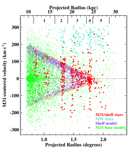
Figure 8: Velocity versus radius as in Fig. 7, but this time including our simulation particles as small points. Particles are selected from a rectangle around the masks as discussed in § 2.2. Purple points show the shelf component formed by the GSS satellite debris, while green points show the component representing M31 itself, which is dominated by the hot smooth spheroid component. Red observed stars are to be compared to the combination of green and purple model points. The orange lines show the analytic envelope discussed in the text.

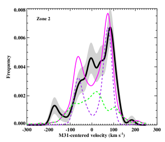
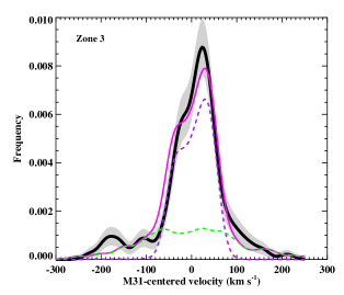
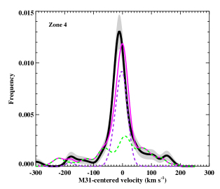
Figure 9: Distribution of M31 stars in velocity within radial zones 2 (left), 3 (center), and 4 (right). Observations and model are kernel-smoothed with a Gaussian of $\sigma=15\,\mbox{km}\,\mbox{s}^{-1}$. Black line: observed M31 stars. The shaded region indicates the $1\sigma$ error band. Magenta line: total distribution in model. Purple line: GSS-related model stars. Green line: M31 galaxy model stars.

In Fig. 8, we again show the velocity versus radius of our stars, this time overlaid on the simulation points from the surrounding area. Purple points show the particles belonging to the GSS-related debris, and green the particles from the base M31 model. For slightly better agreement we have taken the liberty of reducing the radii of the GSS debris particles by 4%, an amount well within the model uncertainties (Fardal et al. in preparation). The agreement between the simulation prediction and observations is striking. The simulated GSS debris lies in a wedge that tapers to a tip at about $1.9^{\circ}$ or 26 kpc, with a strong concentration at the upper edge. The wedge shape results from a caustic in projected velocity that is a consequence of the kinematics of a radial shell (Merrifield & Kuijken, 1998). A large fraction of the observed stars are distributed in a similar pattern.

In the rest of this subsection we will compare the distribution in the radius-velocity plane in more detail. Rather than just making a statistical comparison in arbitrary areas of this plane, we will try to interpret the observed results in a physical way. We first note that the slope of the observed wedge appears to agree with the simulation. Since this slope is related to the gravitational force at the shelf edge (Merrifield & Kuijken, 1998), this suggests our gravitational potential model near radius $20\,\mbox{kpc}$ is reasonable.

The wedge shape of the caustic derived in Merrifield & Kuijken (1998) is triangular, and symmetric around zero systemic velocity. However, this result assumes that the shell star orbits are exactly radial (no angular momentum) and monoenergetic (no velocity dispersion or energy gradient along the flow). In contrast, our simulated shelf material has both angular momentum and an energy gradient along the flow. In the Appendix we derive an analytic expression for the caustic envelope that incorporates both of these effects, as well as second-order terms in the potential and velocity projection. To use this expression we need parameters for the rotation and energy gradient which we now consider.

The mean observed velocities are about $-12\,\mbox{km}\,\mbox{s}^{-1}$ in the large group of cold stars in zone 4 just inside the shelf tip, and $-18\,\mbox{km}\,\mbox{s}^{-1}$ for the smaller group of six stars at slightly larger radius and velocity near zero. Our simulation of the debris similarly assigns small negative velocities for these regions. We estimate the tip velocity in our simulation as about $v_{tip}\approx-20\,\mbox{km}\,\mbox{s}^{-1}$, by taking a sample of particles at the shelf edge. In contrast, a shell model assuming purely radial motions for the stars would find a zero velocity relative to the host, at least to the measurement precision of the systemic velocity which here is roughly $4\,\mbox{km}\,\mbox{s}^{-1}$. The small negative velocity we find in the simulations has clear significance: it represents the effect of angular momentum within the shell particles, which causes motion along the line of sight at the shell edge. We infer the same is true for the observed stars. The direction of the angular momentum results from the specific trajectory assigned to the GSS progenitor in the F07 model, in which stars after passing through the NE Shelf pass behind M31 into the W Shelf, curling toward us at the edge of the shelf. This trajectory is strongly constrained by the need to place the stream and shelves correctly on the sky.

In the simulation, the radial shell giving rise to the W Shelf can be seen to expand over time as stars of higher and higher orbital energies arrive there. This energy gradient is expected on quite general grounds, since stars with higher orbital energies take longer to complete their orbits. The energy gradient skews the wedge shape, increasing the apparent speed of outflowing stars (moving them further from M31’s velocity) and decreasing that of the inflowing stars. The simulated shelf stars mostly lie beyond the midplane, so that outflowing stars have positive velocities and inflowing ones have negative velocities; this results in an upward skew of the wedge.

To combine the skewed velocity envelope given by equation 4 with a global offset due to the angular momentum, we need four parameters. We estimate the shelf expansion speed $v_{sh}=40\,\mbox{km}\,\mbox{s}^{-1}$ from the evolution of the shelf radius in the simulation. We use $v_{rot}=-20\,\mbox{km}\,\mbox{s}^{-1}$ as the result of the line-of-sight projection of the angular momentum, as found above. We choose $r_{sh}=1.97^{\circ}$ to match the observed three-dimensional shelf radius. Finally, from our potential model, we estimate the circular velocity $V_{c}=[GM(r)/r]^{1/2}$ to be $240\,\mbox{km}\,\mbox{s}^{-1}$ at the shell radius. These choices yield the orange lines shown in Fig. 8. Clearly this envelope is a good match to the actual envelope of both the simulation and observed stars. In contrast, a symmetric linear wedge would be a poor fit to the simulated and observed caustic shapes. The upward skew of the wedge towards M31’s center suggests that the simulation correctly places the bulk of the shelf beyond the midplane, so that the positive-velocity stars are the outflowing ones.

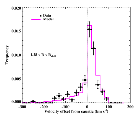
Figure 10: Binned distribution of velocity difference $\Delta v$ from the caustic envelope shown in Fig. 8, as defined in the text. Points with error bars show the observed distribution. The magenta line shows the simulated distribution. The significant jump at zero demonstrates the increase in density just inside the velocity caustic.

In our simulation the M31 disk contributes a small amount to only the innermost mask, but in actuality it is not obvious that any stars with radii and velocities typical of the disk are present in our sample. Therefore our comparison to observations constrains only the shelf and spheroid components. We regard the particular bulge/halo decomposition of the spheroid in our model as somewhat arbitrary, Formally, though, our M31 bulge component dominates the contribution to the surface mass density of the spheroid component out to $25\,\mbox{kpc}$ or $1.8^{\circ}$, in other words nearly the entire region probed by this survey, while the M31 halo component dominates outside that radius.

In Fig. 9 and Fig. 10, we compare in greater detail the distributions of simulated and observed stars in velocity space. We ignore zone 1 in all further comparisons with the simulation, due to the small number of detected stars and the apparent contamination from NGC 205 debris and possibly M31’s disk. (See Fig. 1 and Table 1 for the positions of the radial zones.)

Fig. 9 shows smoothed-kernel representations of observed and simulated stars in the three central zones. In zone 2, there is clearly a steep-sided central component in both observations and simulations, weighted strongly to positive velocities. The simulation is more strongly peaked, and the smaller negative-velocity peak is not clearly distinct in the observations. This could be from an imbalance between our spheroid and shelf components, or a slightly different spatial distribution of shelf stars in this range. In zone 3, the similarity between the simulation and the observations is remarkable. As we approach the edge of the shelf in zone 4, the central component shrinks to a cold peak. The stars in the observed and simulated cold components actually occupy a similar range, but a slightly different distribution of stars within this range produces a small shift in the peak of the smoothed velocity distribution. Clearly, the model provides an essentially correct description of the motions of stars within the shelf.

The sloping caustics shown in Fig. 8 are smeared over velocity in Fig. 9 by the finite range in radius within each zone. Fig. 10 instead shows the velocity distribution in reference to this caustic velocity. We use a histogram rather than kernel smoothing to make a sharp division between stars inside and outside of the caustic. For each observed or simulated star $i$ with $1.28^{\circ}<Y_{i}<1.9^{\circ}$ (i.e., from the inner edge of zone 2 to the shelf boundary), we compute a quantity $\Delta v_{i}=\pm(v_{env,i}-v_{i})$, where $v_{env,i}$ is the nearer of the upper and lower caustics given by the orange lines in Fig. 8 at the star’s radius. We use the plus (minus) sign for stars nearer the upper (lower) caustic. Thus $\Delta v_{i}$ is small and positive for stars just inside the caustic, and small and negative for stars just outside. We show the observed distribution as points with Poisson error bars, and also the result of the simulation as a solid histogram. It is clear that the density jumps by a large amount as one crosses the caustic boundary. The simulated distribution reproduces this distribution rather well, although the fit is poor from a statistical point of view. The same can be said of the $\Delta v$ distributions in individual fields which are not shown here. Not surprisingly, the shelf component is solely responsible for the jump at zero in the simulation, while the M31 component has a broad, smooth distribution.

Now that we have clearly established the presence of both hot smooth and shelf components from their velocity distributions, we use these distributions as templates to find the observed relative strengths of these component. For each of our radial zones, we find the GSS and M31 velocity distributions at the velocities of the observed stars by kernel-smoothing the simulation velocities. We combine these two distributions in proportion to their total masses within the zone, with the GSS component weighted by an additional factor $g_{sat}$. We then compute the total likelihood $\ln L_{sat}$ for the M31 stars being drawn from this distribution, by adding the logarithms of individual velocity distribution values. Repeating this process for a set of values for the weighting factor $g_{sat}$, we find its maximum likelihood estimates and error estimates, and we can compare the likelihood $\ln L_{sat}$ to that of the null model $\ln L_{0}$, where we use only the M31 component and no GSS debris (equivalent to setting $g_{sat}=0$). This test offers very strong evidence for a satellite component in zones 2–4, whereas zones 1 and 5 are ambiguous. (This is not surprising since NGC 205 contaminates the innermost masks, while the outer mask should have very few shelf stars.) In our first set of tests we let $g_{sat}$ take on a different value for each zone. For zones 2, 3, and 4 respectively, we find optimum satellite weights $\ln g_{sat}$ of $-0.8\pm 0.5$, $-0.1\pm 0.3$, and $0.5\pm 0.3$. The log likelihoods relative to the null model are $\ln(L_{sat}/L_{0})$ of 8, 29, and 31, indicating solid detections of the GSS component in each of these zones. If we assume a constant $g_{sat}$ and combine data from all fields, we find $\ln g_{sat}=0.0\pm 0.2$, i.e. the optimum weight of the GSS component is $\bar{g}_{sat}=(1.0\pm 0.2)$ the standard weight in our model. We note that $\ln(L_{sat}/L_{0})=72$, i.e. in a simple likelihood ratio interpretation the kinematic distribution is $>10^{31}$ times more likely to be drawn from the model with a satellite component than that without. This overwhelming statistical requirement for a shelf kinematic component confirms the visual impressions from Figures 8 and 10.

For future work on modeling the GSS, it will be useful to have an estimate of the contribution of the shelf to the M31 stars. The purely photometric sample of Tanaka et al. (2010) shows a steep surface brightness drop at the W Shelf edge, which we can estimate to be roughly 3 magnitudes in their most metal-rich channel by extrapolating their outer surface brightness profile inwards. This would suggest the spheroid constitutes approximately 0.06 of the total metal-rich stars and the shelf component itself about 0.94, albeit with large uncertainties.

The ratio of shelf to spheroid components varies with position, and the average ratio obtained with our somewhat irregular spatial coverage is of no particular interest. Therefore we use the simulations to estimate this ratio averaged over an area defined by the radial range $1.35$–$1.95^{\circ}$ and the azumuthal range 0–$30^{\circ}$ to the SE of the NW minor axis. We compute the satellite-contributed fraction $f_{sat}$ from the numbers of simulation particles in this region in the GSS and M31 components, weighting the GSS count by the satellite weight $\bar{g}_{sat}$. Using the likelihood as a function of $\bar{g}_{sat}$ just described, we find the GSS stars make up $f_{sat}=0.59\pm 0.05$ of the total stars in this region. Better definition of the GSS-related structures can be obtained by focusing on the metal-rich population. If we repeat the likelihood calculation using only metal-rich stars with $[\mathrm{Fe}/\mathrm{H}]>-0.75$ to constrain $g_{sat}$, we require a higher weight of $\bar{g}_{sat}=1.34\pm 0.37$. This yields a higher satellite fraction of $f_{sat}=0.84\pm 0.05$ for this subset of stars. (This suggests that the shelf is more metal-rich than the spheroid, which we discuss in more detail later.) These estimates are the most precise determinations yet of the ratio between the shelf and spheroid, and should be very useful in constraining future models of the GSS.

The observed velocities appear somewhat asymmetric about the origin; most noticeably, the strong enhancement at $R=1.33^{\circ}$, $v=75\,\mbox{km}\,\mbox{s}^{-1}$ is not matched by an equally strong clump at $-75\,\mbox{km}\,\mbox{s}^{-1}$. The model shelf component shows an asymmetry in the same direction (compare the strengths of the upper and lower caustics in Figures 8 and 10). The simulated shelf stars lie beyond the midplane, and we have argued above the observed stars must as well due to the skew of the wedge in $r$-$v$ space. Therefore the positive velocity stars are outgoing and the negative velocity stars are infalling. The ratio of these two components tests the density gradient along the stream, since the infalling stars have larger orbital phase.

To test the model versus the data in a more precise way we restrict our attention to zones 2 and 3, which have a large fraction of shelf stars but are far enough away from the edge that the precise dividing line between outgoing and infalling stars is not important. In the simulation, the outgoing stars (classed as such by their actual 3-d radial velocities) make up $(67\pm 1)$% of the shelf stars within this region. The dividing line between outgoing and infalling stars is reached here at $-8\,\mbox{km}\,\mbox{s}^{-1}$. We use the GSS and M31 velocity distributions, along with the maximum likelihood satellite debris weight factor of $f_{sw}=0.71$, to assign a GSS mixing fraction to each observed star. We can then estimate the number of outgoing and infalling GSS stars by summing up these mixing fractions above and below the dividing line of $-8\,\mbox{km}\,\mbox{s}^{-1}$. The observed outgoing fraction is $70\pm 3$%, in excellent agreement with the simulation. The density therefore falls off steeply with increasing orbital phase. If we accept that the stream density should rise when approaching the phase of the progenitor, then this demonstrates the shelf lies at a larger orbital phase than the main body of the progenitor, as in our model.

3.3 Metallicity of shelf and spheroid components

Our maximum-likelihood weighting of GSS and M31 components over all zones produces for each observed star a mixing fraction, that is, a probability that the star is from one component or the other. We now use these mixing fractions to estimate the metallicity distributions of the individual components.

In Fig. 11 we show the metallicity distribution for the entire sample of M31 stars, kernel-smoothed with a Gaussian of dispersion 0.1 dex. Dashed colored lines show the contribution of the individual components, where each star contributes an amount proportional to its mixing fraction for a given component and is kernel-smoothed as before. It is clear that the GSS debris has higher metallicity on average than the smooth spheroid.

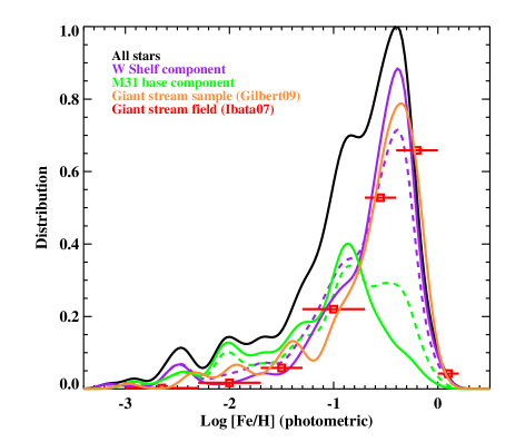
Figure 11: Kernel-smoothed distribution of our W Shelf sample stars in metallicity (solid black curve). The dashed curves indicate the contribution of the shelf (purple) and M31 proper (green) components, using the initial decomposition based on kinematics. The solid curves with the same colors indicate the contributions using the mixing fractions based on both kinematics and metallicity. The observed metallicity distribution of stars within the GSS itself, about 100 kpc to the south, is shown by the orange kernel-smoothed curve for Gilbert et al. (2009), and by the squares with error bars for Ibata et al. (2007).

Our kinematic separation of the stellar components is far from complete—there are many stars with significant mixing fractions in both components, meaning the metallicity distributions of the components are still to some degree mixed together. This mixing can be reversed by applying the metallicity distribution as an additional criterion in computing the mixing fractions. Here we assume that metallicity is independent of position and velocity throughout our observed region. Starting with the original mixing fractions from kinematics alone, we compute the metallicity distributions of each component and use it as an additional factor in the likelihood of a star being from that component. We then recompute kernel-smoothed metallicity distributions from the new mixing fractions, and iterate this process until the mixing fractions converge. In technical jargon, this procedure involves a non-parametric mixture model with prior fuzzy classifications on all the sample points, which we solve for the mixture components using an expectation-maximization algorithm. The result is shown as the solid purple and green curves in Fig. 11. This algorithm always amplifies the differences between the original component distributions. It naturally amplifies noise as well, so we constructed mock samples from our simulation of similar size to the observational sample and tested the separation using the remaining simulation particles to define the components. We found that at our sample size, the algorithm does a good job of recovering the original component distributions without introducing much visible noise.

Our final metallicity distributions in Fig. 11 show an even clearer separation of the satellite debris and smooth spheroid components. The mean metallicities are $-0.7$ for the satellite debris and $-1.2$ for the spheroid component, for a typical difference of $0.5$ dex in $[\mathrm{Fe}/\mathrm{H}]$. The spheroid metallicity has a similar mean and dispersion to that found in the smooth, dynamically hot spheroid population at slightly larger radii (30–$33\,\mbox{kpc}$) on the opposite side of M31 by Kalirai et al. (2006a).

The figure also illustrates the distribution of metallicity within the GSS itself, from the kinematic sample of Gilbert et al. (2007) and the ground-based photometry of Ibata et al. (2007). The Gilbert et al. (2007) sample has advantages of kinematic selection and identical reduction procedures to those employed in our W Shelf sample, but in truth the two GSS distributions are quite similar. The W Shelf debris component shows remarkable agreement with these GSS samples, obtained in a region $\sim\!100\,\mbox{kpc}$ away.

4 DISCUSSION

The observations presented here reveal two main components besides the foreground contaminants from the MW: a hot smooth spheroid with a roughly Gaussian velocity profile, and a shelf component with kinematics matching that of a radial shell. The kinematic properties of the shelf component match very well to a simulation of the GSS’s formation. The metallicity distributions of the two components are distinct, with the shelf having higher mean metallicity and matching very well to observations of the GSS. This agrees with the earlier conclusion of Tanaka et al. (2010), who compared purely photometric samples in the W Shelf and GSS regions and also found them to be nearly identical.

Some caution is warranted when drawing connections between tidal structures based on their stellar populations. Different tidal progenitors can have similar metallicity distributions, and a single tidal structure can have gradients along it, as seems to be the case for the Sagittarius stream (Chou et al., 2007). Indeed, the GSS itself seems to have a metallicity gradient from its core to its less dense “cocoon” on the SE side (Ibata et al., 2007). The models of Fardal et al. (2008) reproduce such a gradient by assuming a gradient in the progenitor. Importantly, however, neither observations nor models suggest a strong gradient along the stream, especially for regions separated by a comparable amount from the progenitor’s core. In the F07 model, the W Shelf leads and the GSS trails the current core location by similar amounts. Thus it is reasonable to connect the two structures by their stellar populations.

The precision of resolved-star spectroscopy allows a remarkable range of conclusions to be drawn from the velocity structure. We showed the observations agree not just with the overall wedge pattern of the shelf component, but also agree with more subtle aspects. The ratio of upper and lower caustic populations, the velocity shift at the tip of the wedge from M31’s systemic velocity, and the slightly skewed shape of the wedge all have physical meaning in the simulations, and the data are in good agreement with the simulation trends for all these aspects. The high precision of the kinematic data encourages use in constraining our satellite model further. For example, we already had to adjust the radii in the model very slightly, an adjustment well within the constraints posed by other observations of the stream debris.

Together, the metallicity and kinematics make a strong case that the W Shelf indeed originates from the same disruption event that produced the GSS. The structure around M31 is still incompletely understood. In particular, part of the GSS region shows a second stream offset by $+100\,\mbox{km}\,\mbox{s}^{-1}$ from the GSS itself, which is currently unexplained by our models. Is it possible that the W Shelf itself results from a similar, but independent accretion event to that which formed the GSS? The rich variety of observational features matched by our simulations suggests that this is unlikely. However, further confirmation of the model is worthwhile. The next test for the model is likely to come in the NE Shelf region, where the model places the bulk of the GSS-related material. In this region our model predicts a similar wedge kinematic pattern to that in the W Shelf (see F07). We have argued that negative-velocity (outflowing) stars have been detected already in this region, but the detection of a positive-velocity (returning) component will provide a clear connection between all parts of the GSS model. The progenitor’s total stellar mass in our model is roughly comparable to that of the LMC, and adding up the stellar mass of all the GSS-related features will provide another test of the model.

The smooth spheroid component is consistent with that found elsewhere in M31. The velocity distribution agrees in its mean and dispersion with that found previously on the opposite side of M31’s disk, as does the metallicity distribution. This provides strong evidence for a symmetric, mostly virialized hot component at intermediate radii. It may be a bit simplistic to call this inner spheroid “smooth”, as evidenced by the $-175\,\mbox{km}\,\mbox{s}^{-1}$ clump of stars with a small range of metallicities we found in § 3. This is not unexpected in theories of galaxy halo formation, as fine-grained structure can linger in phase space and stellar population space far longer than is apparent in morphology (e.g. Helmi & White, 1999; Johnston et al., 2008). However, at a minimum it is made up of a very large number of components below the threshold of individual detectability spread over a large velocity range, as opposed to the cold monolithic kinematic pattern of the shelf component.

It is clear that M31’s inner halo remains a confusing region, and much work remains to be done to decompose it into kinematically distinct components. The extent of the W Shelf in particular remains to be mapped, as in star-count maps it becomes confused with M31’s outer disk on both the NW and SE sides. Extrapolating from progress in the last decade, we expect rapid growth in our understanding of M31’s halo from the combination of large imaging surveys with spectroscopic surveys such as we have presented here.

The wedge pattern detected in Fig. 8 is to our knowledge the first time a radial shell kinematic pattern (Merrifield & Kuijken, 1998) has been clearly detected in any galaxy, although features of the pattern were suggested earlier in F07. It is also the first spiral galaxy found to exhibit a system of multiple shell structures, though recently NGC 4651 has been found to exhibit similar structures (Martínez-Delgado et al., 2010). Shell systems are of course common in elliptical galaxies (e.g. Malin & Carter, 1983; Merrifield & Kuijken, 1998; Canalizo et al., 2007). Our results offer inspiration for the future detection of shell kinematics in more distant galaxies and its use in measuring their gravitational potential, using either bright tracers such as planetary nebulae or globulars or else RGB stars detected with a future generation of telescopes.

Appendix A Physics of less-idealized shells — expansion, rotation, and velocity dispersion

Here we derive some results on the kinematics of non-ideal shells, for use both in the preceding analysis of the W Shelf and in understanding future observations of other stellar shells.

Merrifield & Kuijken (1998) derived the observable kinematics of a stellar shell in the idealized case of a monoenergetic, perfectly radial flow of stars in a gravitational field of uniform strength. In the same approximation, F07 derived the shell surface density in terms of the gravitational potential and flow rate of stars through the shell. Both papers discussed several physical and observational aspects of stellar shells besides those mentioned in this paper. However, here we need several results not mentioned in either paper.

To establish notation, we repeat the argument of Merrifield & Kuijken (1998) here. Denote the three-dimensional radius as $r$ and the projected radius as $R$. Consider a shell of fixed radius $r_{sh}$, with stars of constant orbital energy flowing out to $r_{sh}$ and back, and for convenience let us consider only the stars on the far side of the host. Write $b=r/r_{sh}$, $\beta=R/r_{sh}$. Let the gravitational field have a constant strength $g$; then at the shell edge the circular velocity is $V_{c}=(gr_{sh})^{1/2}$. The radial velocity of the stars is given by $v_{r}^{2}=2g(r_{sh}-r)=2V_{c}^{2}(1-b)$. The line-of-sight velocity is instead given by $v_{los}=(z/r)v_{r}$, where $z$ is the distance relative to the host distance. (Here we neglect perspective effects.) Near the shell edge we can to first order take $z/r=[(r^{2}-R^{2})/r^{2}]^{1/2}\approx[2(b-\beta)]^{1/2}$. Then $v_{los}=\pm 2V_{c}(b-\beta)^{1/2}(1-b)^{1/2}$. The magnitude of the velocity is maximized at $b=(1+\beta)/2$, implying the envelope of $v_{los}$ is given by $v_{env}=\pm V_{c}(1-\beta)=\pm V_{c}(r_{sh}-R)/r_{sh}$. Here the top and bottom signs apply to the outgoing and incoming stars respectively. Thus projecting the velocities has squashed the sideways parabola of $v_{r}(r)$ into a wedge. The gradual turnover in $v_{los}$ around its maximum gives the distribution of stars in velocity space a caustic or horn shape. A similar argument applies to stars on the near side of the host, with the roles of the positive and negative caustics reversed.

While undoubtedly useful as a first approximation, this contains one fundamental problem: the radial shell exists only because stars have different orbital energies and hence arrive at the shell edge at different times. The gradient is invariably in the sense that later-arriving stars have higher energies, because larger orbital energy increases the orbital period. We can handle this problem simply by incrementing the outward velocity of all stars in the shell by the same amount.

$$(v_{r}-v_{sh})^{2}=2g(r_{sh}-r)=2V_{c}^{2}(1-b)$$ (1)

If we label each star by the time $t_{p}$ it arrives at the shell boundary, its specific energy becomes $E=v_{sh}^{2}/2+r_{sh}g+v_{sh}gt_{p}$. The energy gradient can then be expressed as

$$dE/d(t_{p})=v_{sh}g=v_{sh}V_{c}^{2}/r_{sh}\;.$$ (2)

(As argued above, $dE/d(t_{p})$ and $v_{sh}$ are both in general positive.) This shows the expansion speed of the shell is proportional to the gradient in orbital energy along the stream.

We can again solve for the maximum line-of-sight velocity at a given projected radius. Defining $\epsilon\equiv v_{sh}/(gr_{sh})^{1/2}=v_{sh}/V_{c}$, $\delta=1-\beta$, and $\nu=(\epsilon/8)([16\delta+\epsilon^{2}]^{1/2}-\epsilon)$, and differentiating to find the extremum, we find an envelope velocity of

$$v_{env}=V_{c}(\delta\pm\nu)^{1/2}[\epsilon\pm(\delta\mp\nu)^{1/2}]\;.$$ (3)

This results in an envelope in $r$-$v_{los}$ space that is shifted upwards relative to the monoenergetic case at most radii, with an increasingly skewed shape approaching the shelf radius so that the tip remains at zero velocity. This is a natural result of the outgoing stars (upper branch of the envelope) having higher energies and thus greater velocities. For lines of sight outside the radius where the “returning” particles have zero radial velocity, given by $(2\delta)^{1/2}=\epsilon$, there is no returning caustic and the minimum envelope velocity of zero is reached at the midplane. The tip remains fixed at zero velocity because the radial velocity at the shelf edge lies perpendicular to the line of sight. If the shell material instead lies on the near side of the host galaxy, then the energy gradient instead skews the envelope in the negative-velocity direction, with the tip again fixed at zero. If the shell material fills both sides of the galaxy, the degeneracy of the near and far side envelopes is broken and both envelopes will be present, offset from each other at all $r<r_{sh}$.

Since the expansion velocity is typically small compared to $V_{c}$, it is more useful to take a perturbative approach, which allows us to incorporate second-order effects in the gravitational potential and velocity projection. To this order we can write $z/r\approx\sqrt{2}(\delta-D)^{1/2}(1+\frac{3}{4}D-\frac{1}{4}\delta)$. with $D\equiv 1-b$. We assume a flat rotation curve, in which case $\Phi(r)-\Phi(r_{sh})\approx-V_{c}^{2}D(1+\frac{1}{2}D)$. To this order we can assume the extremum is reached at $D=\delta/2$, the lowest-order solution. Combining the various factors, we reach our final approximation

$$v_{env}\approx V_{c}\delta^{1/2}(1+\frac{1}{8}\delta)\left[\epsilon\pm\delta^{1/2}(1+\frac{1}{8}\delta)\right]\;.$$ (4)

The first factor of $(1+\frac{1}{8}\delta)$ is contributed by the projection factor, and the second (in the case of a flat rotation curve only) by the potential.

In the case of the W Shelf, as will be true in most cases, the shell material is not purely radial but instead has significant angular momentum. This affects the observed velocities by shifting the envelope up or down. We apply this as a global shift to the entire envelope in Fig. 8. A higher-order analysis would take into account the radial dependence of tangential velocity and derive the envelope shift by rederiving the caustic analysis above, but the simple shift used here appears accurate enough for our purposes.

As a final exercise, we estimate the smearing in the stellar velocities near the caustic edge induced by a local radial velocity dispersion $\sigma_{r}$ of the stream particles. This dispersion might be left over from initial conditions in a young stream like that discussed here, or else result from interaction with LCDM substructure (Carlberg, 2009) in an older one. To first order we can estimate the observed dispersion from the monoenergetic picture, where the projection factor at the velocity caustic is $z/r=(1-\beta)^{1/2}$. Thus we expect the envelope edge to be blurred by an amount

$$\sigma_{los}=[(r_{sh}-R)/r_{sh})]^{1/2}\sigma_{r}\;.$$ (5)

References

- Brown et al. (2008) Brown T. M., Beaton R., Chiba M., Ferguson H. C., Gilbert K. M., Guhathakurta P., Iye M., Kalirai J. S., Koch A., Komiyama Y., Majewski S. R., Reitzel D. B., Renzini A., Rich R. M., Smith E., Sweigart A. V., Tanaka M., 2008, ApJ, 685, L121
- Brown et al. (2003) Brown T. M., Ferguson H. C., Smith E., Kimble R. A., Sweigart A. V., Renzini A., Rich R. M., VandenBerg D. A., 2003, ApJ, 592, L17
- Brown et al. (2009) Brown T. M., Smith E., Ferguson H. C., Guhathakurta P., Kalirai J. S., Kimble R. A., Renzini A., Rich R. M., Sweigart A. V., Vanden Berg D. A., 2009, ApJS, 184, 152
- Brown et al. (2007) Brown T. M., Smith E., Ferguson H. C., Guhathakurta P., Kalirai J. S., Rich R. M., Renzini A., Sweigart A. V., Reitzel D., Gilbert K. M., Geha M., 2007, ApJ, 658, L95
- Brown et al. (2006) Brown T. M., Smith E., Guhathakurta P., Rich R. M., Ferguson H. C., Renzini A., Sweigart A. V., Kimble R. A., 2006, ApJ, 636, L89
- Butler & Martínez-Delgado (2005) Butler D. J., Martínez-Delgado D., 2005, AJ, 129, 2217
- Canalizo et al. (2007) Canalizo G., Bennert N., Jungwiert B., Stockton A., Schweizer F., Lacy M., Peng C., 2007, ApJ, 669, 801
- Carlberg (2009) Carlberg R. G., 2009, ApJ, 705, L223
- Chapman et al. (2006) Chapman S. C., Ibata R., Lewis G. F., Ferguson A. M. N., Irwin M., McConnachie A., Tanvir N., 2006, ApJ, 653, 255
- Choi et al. (2002) Choi P. I., Guhathakurta P., Johnston K. V., 2002, AJ, 124, 310
- Chou et al. (2007) Chou M., Majewski S. R., Cunha K., Smith V. V., Patterson R. J., Martínez-Delgado D., Law D. R., Crane J. D., Muñoz R. R., Garcia López R., Geisler D., Skrutskie M. F., 2007, ApJ, 670, 346
- Courteau et al. (2011) Courteau S., Widrow L. M., McDonald M., Guhathakurta P., Gilbert K. M., Zhu Y., Beaton R. L., Majewski S. R., 2011, ApJ, 739, 20
- de Vaucouleurs et al. (1991) de Vaucouleurs G., de Vaucouleurs A., Corwin Jr. H. G., Buta R. J., Paturel G., Fouque P., 1991, Third Reference Catalogue of Bright Galaxies. Springer-Verlag Berlin Heidelberg New York
- Durrell et al. (2001) Durrell P. R., Harris W. E., Pritchet C. J., 2001, AJ, 121, 2557
- Fardal et al. (2006) Fardal M. A., Babul A., Geehan J. J., Guhathakurta P., 2006, MNRAS, 366, 1012
- Fardal et al. (2008) Fardal M. A., Babul A., Guhathakurta P., Gilbert K. M., Dodge C., 2008, ApJ, 682, L33
- Fardal et al. (2007) Fardal M. A., Guhathakurta P., Babul A., McConnachie A. W., 2007, MNRAS, 380, 15
- Ferguson et al. (2002) Ferguson A. M. N., Irwin M. J., Ibata R. A., Lewis G. F., Tanvir N. R., 2002, AJ, 124, 1452
- Geehan et al. (2006) Geehan J. J., Fardal M. A., Babul A., Guhathakurta P., 2006, MNRAS, 366, 996
- Geha et al. (2006) Geha M., Guhathakurta P., Rich R. M., Cooper M. C., 2006, AJ, 131, 332
- Gilbert et al. (2007) Gilbert K. M., Fardal M., Kalirai J. S., Guhathakurta P., Geha M. C., Isler J., Majewski S. R., Ostheimer J. C., Patterson R. J., Reitzel D. B., Kirby E., Cooper M. C., 2007, ApJ, 668, 245
- Gilbert et al. (2006) Gilbert K. M., Guhathakurta P., Kalirai J. S., Rich R. M., Majewski S. R., Ostheimer J. C., Reitzel D. B., Cenarro A. J., Cooper M. C., Luine C., Patterson R. J., 2006, ApJ, 652, 1188
- Gilbert et al. (2009) Gilbert K. M., Guhathakurta P., Kollipara P., Beaton R. L., Geha M. C., Kalirai J. S., Kirby E. N., Majewski S. R., Patterson R. J., 2009, ApJ, 705, 1275
- Guhathakurta et al. (2005) Guhathakurta P., Ostheimer J. C., Gilbert K. M., Rich R. M., Majewski S. R., Kalirai J. S., Reitzel D. B., Patterson R. J., 2005, ArXiv e-prints, astro-ph/0502366
- Guhathakurta et al. (2006) Guhathakurta P., Rich R. M., Reitzel D. B., Cooper M. C., Gilbert K. M., Majewski S. R., Ostheimer J. C., Geha M. C., Johnston K. V., Patterson R. J., 2006, AJ, 131, 2497
- Hammer et al. (2010) Hammer F., Yang Y. B., Wang J. L., Puech M., Flores H., Fouquet S., 2010, ApJ, 725, 542
- Helmi & White (1999) Helmi A., White S. D. M., 1999, MNRAS, 307, 495
- Ibata et al. (2005) Ibata R., Chapman S., Ferguson A. M. N., Lewis G., Irwin M., Tanvir N., 2005, ApJ, 634, 287
- Ibata et al. (2001) Ibata R., Irwin M., Lewis G., Ferguson A. M. N., Tanvir N., 2001, Nat, 412, 49
- Ibata et al. (2007) Ibata R., Martin N. F., Irwin M., Chapman S., Ferguson A. M. N., Lewis G. F., McConnachie A. W., 2007, ApJ, 671, 1591
- Irwin et al. (2005) Irwin M. J., Ferguson A. M. N., Ibata R. A., Lewis G. F., Tanvir N. R., 2005, ApJ, 628, L105
- Johnston et al. (2008) Johnston K. V., Bullock J. S., Sharma S., Font A., Robertson B. E., Leitner S. N., 2008, ApJ, 689, 936
- Kalirai et al. (2006a) Kalirai J. S., Gilbert K. M., Guhathakurta P., Majewski S. R., Ostheimer J. C., Rich R. M., Cooper M. C., Reitzel D. B., Patterson R. J., 2006a, ApJ, 648, 389
- Kalirai et al. (2006b) Kalirai J. S., Guhathakurta P., Gilbert K. M., Reitzel D. B., Majewski S. R., Rich R. M., Cooper M. C., 2006b, ApJ, 641, 268
- Koch et al. (2008) Koch A., Rich R. M., Reitzel D. B., Martin N. F., Ibata R. A., Chapman S. C., Majewski S. R., Mori M., Loh Y.-S., Ostheimer J. C., Tanaka M., 2008, ApJ, 689, 958
- Libeskind et al. (2011) Libeskind N. I., Knebe A., Hoffman Y., Gottlöber S., Yepes G., 2011, MNRAS, 418, 336
- Malin & Carter (1983) Malin D. F., Carter D., 1983, ApJ, 274, 534
- Martínez-Delgado et al. (2010) Martínez-Delgado D., Gabany R. J., Crawford K., Zibetti S., Majewski S. R., Rix H.-W., Fliri J., Carballo-Bello J. A., Bardalez-Gagliuffi D. C., Peñarrubia J., Chonis T. S., Madore B., Trujillo I., Schirmer M., McDavid D. A., 2010, AJ, 140, 962
- McConnachie et al. (2004) McConnachie A. W., Irwin M. J., Lewis G. F., Ibata R. A., Chapman S. C., Ferguson A. M. N., Tanvir N. R., 2004, MNRAS, 351, L94
- McConnachie et al. (2009) McConnachie A. W., et al., 2009, Nat, 461, 66
- Merrett et al. (2003) Merrett H. R., Kuijken K., Merrifield M. R., Romanowsky A. J., Douglas N. G., Napolitano N. R., Arnaboldi M., Capaccioli M., Freeman K. C., Gerhard O., Evans N. W., Wilkinson M. I., Halliday C., Bridges T. J., Carter D., 2003, MNRAS, 346, L62