Revisit relic gravitational waves based on the latest CMB observations

Abstract

According to the CMB observations, Mielczarek (Mielczarek ) evaluated the reheating temperature, which could help to determine the history of the Universe. In this paper, we recalculate the reheating temperature using the new data from WMAP 7 observations. Based on that, we list the approximate solutions of relic gravitational waves (RGWs) for various frequency bands. With the combination of the quantum normalization of RGWs when they are produced and the CMB observations, we obtain the relation between the tensor-to-scalar ratio $r$ and the inflation index $\beta$ for a given scalar spectral index $n_{s}$. As a comparison, the diagram $r-\beta$ in the slow-roll inflation model is also given. Thus, the observational limits of $r$ from CMB lead to the constraints on the value of $\beta$. Then, we illustrate the energy density spectrum of RGWs with the quantum normalization for different values of $r$ and the corresponding $\beta$. For comparison, the energy density spectra of RGWs with parameters based on slow-roll inflation are also discussed. We find that the values of $n_{s}$ affect the spectra of RGWs sensitively in the very high frequencies. Based on the current and planed gravitational wave detectors, we discuss the detectabilities of RGWs.

PACS number: 04.30.-w, 98.80.Es, 98.80.Cq

I Introduction

General relativity and quantum mechanics predict a stochastic background of relic gravitational waves (RGWs) grishchuk1 ; grishchuk ; grishchuk3 ; starobinsky ; Maggiore ; Giovannini , generated during the early inflationary stage. The primordial amplitudes could be determined by the quantum normalization at the time of the wave modes crossing the horizon during the inflation. After that, the evolution of RGWs are mainly determined by a sequence of stages of cosmic expansion including the current acceleration zhang2 ; Zhang4 , since the interaction of RGWs with other cosmic components is typically very weak. Therefore, RGWs carry a unique information of the early Universe, and serve as a probe into the Universe much earlier than the recombination stage. As an interesting source for gravitational wave (GW) detectors, RGWs exist everywhere and anytime unlike GWs radiated by usual astrophysical process. Moreover, RGWs spread a very broad range of frequency, $10^{-18}-10^{10}$ Hz, making themselves become one of the major scientific goals of various GW detectors with different response frequency bands. The current and planed GW detectors contain the ground-based interferometers, such as LIGO ligo1 , Advanced LIGO ligo2 ; advligo , VIRGO virgo ; virgocurve , GEO geo , AIGO Degallaix , LCGT lcgt and ET Punturo ; Hild aiming at the frequency range $10^{2}-10^{3}$ Hz; the space interferometers, such as the future LISA lisa0 ; lisa which is sensitive in the frequency range $10^{-4}-10^{-1}$ Hz, BBO Crowder ; Cutler and DECIGO Kawamura which both are sensitive in the frequency range $0.1-10$ Hz; and the pulsar timing array, such as PPTA PPTA ; Jenet and the planned SKA Kramer with the frequency window $10^{-9}-10^{-6}$ Hz. Besides, there some potential very-high-frequency GW detectors, such as the waveguide detector cruise , the proposed gaussian maser beam detector around GHz fangyu , and the 100 MHz detector with a pair of 75-cm baseline synchronous recycling interferometers Akutsu . Furthermore, the very low frequency portion of RGWs also contribute to the anisotropies and polarizations of cosmic microwave background (CMB) basko , yielding a magnetic type polarization of CMB as a distinguished signal of RGWs. WMAP Peiris ; Spergel ; Hinshaw ; Komatsu , Planck Planck , the ground-based ACTPol Niemack and the proposed CMBpol CMBpol are of this type.

The reheating temperature, $T_{\rm{RH}}$, carries rich information of the early Universe, and relates to the decay rate of the inflation as $T_{\rm{RH}}\propto\sqrt{\Gamma}$ Kolb ; Nakayama Recently, the reheating temperature was evaluated Mielczarek according to the CMB observations by WMAP 7 in the frame of the slow-roll inflation Komatsu . Then, the expansion histories of different stages could be determined subsequently. In this paper, we reevaluate the reheating temperature using the latest observational data from CMB, and adopt the resulting expansion periods of different phases of the Universe as references. The referenced reheating temperature can help us to divide the phases of the Universe definitely. The evolutions of the RGWs at various phases can be determined subsequently, and the primordial amplitude was normalized due to the quantum condition during inflation grishchuk ; grishchuk3 . For the present time, the solutions of RGWs can be obtained for different frequency bands corresponding to the modes re-entered the horizon at different phases. Note that, this model of RGWs is free from the slow-roll inflation. Therefore, the above reheating temperature based on the slow-roll inflation just serves as a reference. On the other hand, the anisotropies due to the tensor metric perturbations (gravitational waves) can be scaled to those due to the observations of the scalar perturbations by introducing a parameter $r$ called tensor-to-scalar ratio. Combining the observations of the CMB and the quantum normalization of RGWs when they are generated, a constraint condition is arrived between the ratio $r$, the inflation index $\beta$, and the index $\beta_{s}$ describing the expansion behavior of the Universe from the end of inflation to the reheating process. For the chaotic inflation with a quadratic potential $V=\frac{1}{2}m^{2}\phi^{2}$, which means $\beta_{s}=1$, the diagram $r-\beta$ will be illustrated for given values of the scalar spectral index $n_{s}$. The resulting spectra of RGWs for different values of $r$ the corresponding $\beta$ will be demonstrated. For comparison, we will also discuss the spectra of RGWs with the values of $r$ and $\beta$ predicted by the slow-roll inflation itself. To this end, the spectra of RGWs given by different models and different parameters will confront the various current and planed GW detectors.

The outline of this paper is as follows. In Sec. II, we recalculate the reheating temperature using the latest data from CMB and plot it as a function of the scalar spectral index. Based on that, the scale factor $a(\tau)$ is specified for consecutive stages of cosmic expansion. In section III, we present the resulting approximate solutions of the spectrum of RGWs for various frequency bands. In section IV, the spectra of RGWs for different values of parameters are shown and some comparisons between the spectra based on quantum normalization and those based on slow-roll inflation will be given. Some discussions are summarized in Sec. V. Throughout this paper, we use the units $c=\hbar=k_{B}=1$. Indices $\lambda$, $\mu$, $\nu$,… run from 0 to 3, and $i$, $j$, $k$,… run from 1 to 3.

II The expansion history of the universe

For a spatially flat ($k=0$) universe the Robertson-Walker spacetime has a metric

$$ds^{2}=a^{2}(\tau)[-d\tau^{2}+\delta_{ij}dx^{i}dx^{j}],$$ (1)

where $\tau$ is the conformal time, and the scale factor $a(\tau)$ is described by the following successive stages grishchuk ; zhang2 :

The inflationary stage:

$$a(\tau)=l_{0}|\tau|^{1+\beta},\,\,\,\,-\infty<\tau\leq\tau_{1},$$ (2)

where the inflation index $\beta$ is an important model parameter. The special case of $\beta=-2$ corresponds the exact de Sitter expansion. However, both the model-predicted and the observed results indicate that the value of $\beta$ can differ slightly from $-2$.

The preheating stage :

$$a(\tau)=a_{z}|\tau-\tau_{p}|^{1+\beta_{s}},\,\,\,\,\tau_{1}\leq\tau\leq\tau_{s},$$ (3)

where the parameter $\beta_{s}$ is usually taken as a constant. After inflation, the inflation field undergoes coherent oscillations at the bottom of potential well. The reheating process takes place the Hubble parameter $H$ falls to the value of the inflation decay rate $\Gamma_{\phi}$, if we assume that the reheating is instantaneous. Then the preheating process lasts from the end of inflation to the happening of reheating. Below, we will discuss the value of $\beta_{s}$ in detail.

The radiation-dominant stage :

$$a(\tau)=a_{e}(\tau-\tau_{e}),\,\,\,\,\tau_{s}\leq\tau\leq\tau_{2}.$$ (4)

The matter-dominant stage:

$$a(\tau)=a_{m}(\tau-\tau_{m})^{2},\,\,\,\,\tau_{2}\leq\tau\leq\tau_{E}.$$ (5)

The accelerating stage up to the present time $\tau_{0}$ zhang2 :

$$a(\tau)=l_{H}|\tau-\tau_{a}|^{-\gamma},\,\,\,\,\tau_{E}\leq\tau\leq\tau_{0},$$ (6)

where $\gamma$ is a $\Omega_{\Lambda}$-dependent parameter, and $\Omega_{\Lambda}$ is the energy density contrast. To be specific, we take $\gamma\simeq 1.97$ zhangtong for $\Omega_{\Lambda}=0.73$ Komatsu in this paper. It is convenient to choose the normalization $|\tau_{0}-\tau_{a}|=1$, i.e., the present scale factor $a(\tau_{0})=l_{H}$. From the definition of the Hubble constant, one has $l_{H}=\gamma/H_{0}$, where $H_{0}=100\,h$ km s^-1Mpc^-1 is the present Hubble constant. We take $h\simeq 0.704$ Komatsu throughout this paper. Imposing $\beta$ and $\beta_{s}$ as model parameters, only 12 constants remain in all the expressions of the scale factor. The continuity of $a(\tau)$ and $a^{\prime}(\tau)$ at the four given joining points $\tau_{1}$, $\tau_{s}$, $\tau_{2}$ and $\tau_{E}$ provide 8 constraints. If we also know the expansion history of various stages, i.e., the definite values of $\zeta_{1}\equiv{a(\tau_{s})}/{a(\tau_{1})}$, $\zeta_{s}\equiv{a(\tau_{2})}/{a(\tau_{s})}$, $\zeta_{2}\equiv{a(\tau_{E})}/{a(\tau_{2})}$, and $\zeta_{E}\equiv{a(\tau_{0})}/{a(\tau_{E})}$, all the 12 constants can be fixed completely Miao .

The late-time universe is well know. For the $\Lambda$CDM model, the density of dark energy, which drives the accelerating expansion of the universe, is constant. Based on that, one easily has $\zeta_{E}=1+z_{E}=({\Omega_{\Lambda}}/{\Omega_{m}})^{1/3}\simeq 1.4$, where $z_{E}$ is the redshift when the accelerating expansion begins. For the duration of the matter-dominated stage, we get straightforwardly $\zeta_{2}=\frac{a(\tau_{0})}{a(\tau_{2})}\frac{a(\tau_{E})}{a(\tau_{0})}=(1+z_{eq})\zeta_{E}^{-1}$ with $z_{eq}=3240$ Komatsu . However, the histories of the radiation-dominated stage and the preheating stage are not known well. Recently, Mielczarek Mielczarek proposed a method to evaluate the reheating temperature, $T_{\rm{RH}}$, under the frame of the slow-roll inflation model combing the observations from WMAP. Using this method, one can easily obtain the following expression:

$$T_{\rm{RH}}=\frac{15\,m_{Pl}}{8\,g_{\star s}\,\pi^{7/2}}\sqrt{\frac{1-n_{s}}{A_{s}}}\left(\frac{k_{0}^{p}}{T_{\rm{CMB}}}\right)^{3}\exp{\left(\frac{6}{1-n_{s}}\right)}$$ (7)

where $m_{Pl}\equiv 1/\sqrt{G}=1.22\cdot 10^{19}$ GeV is the Plank mass, $g_{\star s}=3.91$ counts the effective number of photons plus three species of massless neutrinos contributing to the radiation entropy during the recombination Yuki , $n_{s}$ is the scalar spectral index, $A_{s}=(2.43\pm 0.11)\cdot 10^{-9}$ is the amplitude of the scalar power spectrum at the pivot physical wavenumber $k_{0}^{p}=0.002$ Mpc^-1 here , and $T_{\rm{CMB}}=2.725\ {\rm{K}}=2.348\cdot 10^{-13}$ GeV is the present temperature of CMB. Note that, in deriving Eq. (7), the approximation of $\beta\approx-2$ was used, and a quadratic potential $V(\phi)=\frac{1}{2}m^{2}\phi^{2}$ of the scalar field, where the scalar mass $m$ can be fixed to be $\sim 10^{13}$ GeV Kuroyanagi ; Mielczarek by CMB observations, was assumed. As analyzed by Turner Turner , during the prehearting stage, when the oscillating frequency of $\phi$ is much greater than the expansion rate of the Universe, the coherent scalar field oscillations behave like a fluid with $p=w\rho$, where the equation of state $w$ depends upon the form of the scalar potential $V(\phi)$. Say $V(\phi)=\lambda\phi^{n}$, one has $w=\frac{n-2}{n+2}$ and $\rho$ decreases as $a^{-6n/(n+2)}$. For $V(\phi)=\frac{1}{2}m^{2}\phi^{2}$, i.e., $n=2$, one has $w=0$ and $\rho\propto a^{-3}$. This result was also verified by Martin and Ringeval martin using numerical method, and it was found that the average $w$ never deviates from zero exceeding $8\%$. Hence, during the evolution of the prehearting stage, the energy density drops approximately in the same way as the matter-dominated Universe Starobinsky2 , and the scale factor evolves as $a(t)\propto t^{2/3}$, which means $\beta_{s}=1$ from Eq. (3). So, in the following we set $\beta_{s}=1$ except that we write it explicitly. Moreover, the following relations in the slow-roll inflation LiddleA :

$$\epsilon\equiv\frac{m^{2}_{Pl}}{16\pi}\left(\frac{V^{\prime}}{V}\right)^{2},\qquad\eta\equiv\frac{m^{2}_{Pl}}{8\pi}\left(\frac{V^{\prime\prime}}{V}\right),\qquad n_{s}=1-6\epsilon+2\eta,$$ (8)

were also used in deriving Eq. (7). According to the observations of WMAP 7, Mielczarek obtained $T_{\rm{RH}}=3.5\cdot 10^{6}$ GeV with $n_{s}=0.963\pm 0.012$ and $A_{s}=2.441^{+0.088}_{-0.092}\cdot 10^{-9}$, assuming $g_{\star s}=2$ being the effective number of relativistic degree of freedom only contributed by photons during recombination. One can recalculate $T_{\rm{RH}}$ using the updated data given by WMAP 7 Komatsu . For example, for WMAP Seven-year Mean, $n_{s}=0.967\pm 0.014$, one has $T_{\rm{RH}}\simeq 5.8\cdot 10^{14}\ {\rm GeV}$ with a relative uncertainty $\sigma(T_{\rm{RH}})/T_{\rm{RH}}\approx 77$; and for WMAP Seven-year ML, $n_{s}=0.966$, one has $T_{\rm{RH}}\simeq 2.8\cdot 10^{12}\ {\rm GeV}$. Thus, one can see that $T_{\rm{RH}}$ depends on the value of $n_{s}$ very sensitively. This is because the expression of $T_{\rm{RH}}$ contains a exponential factor $\exp{(\frac{6}{1-n_{s}})}$, which is dependent on the value of $n_{s}$ very sensitively. For a more general potential with power-law form $V=\lambda\phi^{n}$, one can easily obtain the $e$-foldingor number $N_{\rm{obs}}\simeq\frac{n+2}{2(1-n_{s})}$ using Eq. (14) in Ref. Mielczarek , and in turn the resultant $T_{\rm{RH}}$ has an exponential factor $\exp{(\frac{3(n+2)}{2(1-n_{s})})}$. For example, $n=4$, which implies $w=1/3$ and $\beta_{s}=0$, $T_{\rm{RH}}$ contains a factor $\exp{(\frac{9}{1-n_{s}})}$. Therefore, $T_{\rm{RH}}$ also depends on the power index $n$, and in turn, on $\beta_{s}$ very sensitively. We plot the reheating temperature as a function of the scalar spectral index in Fig. 1.

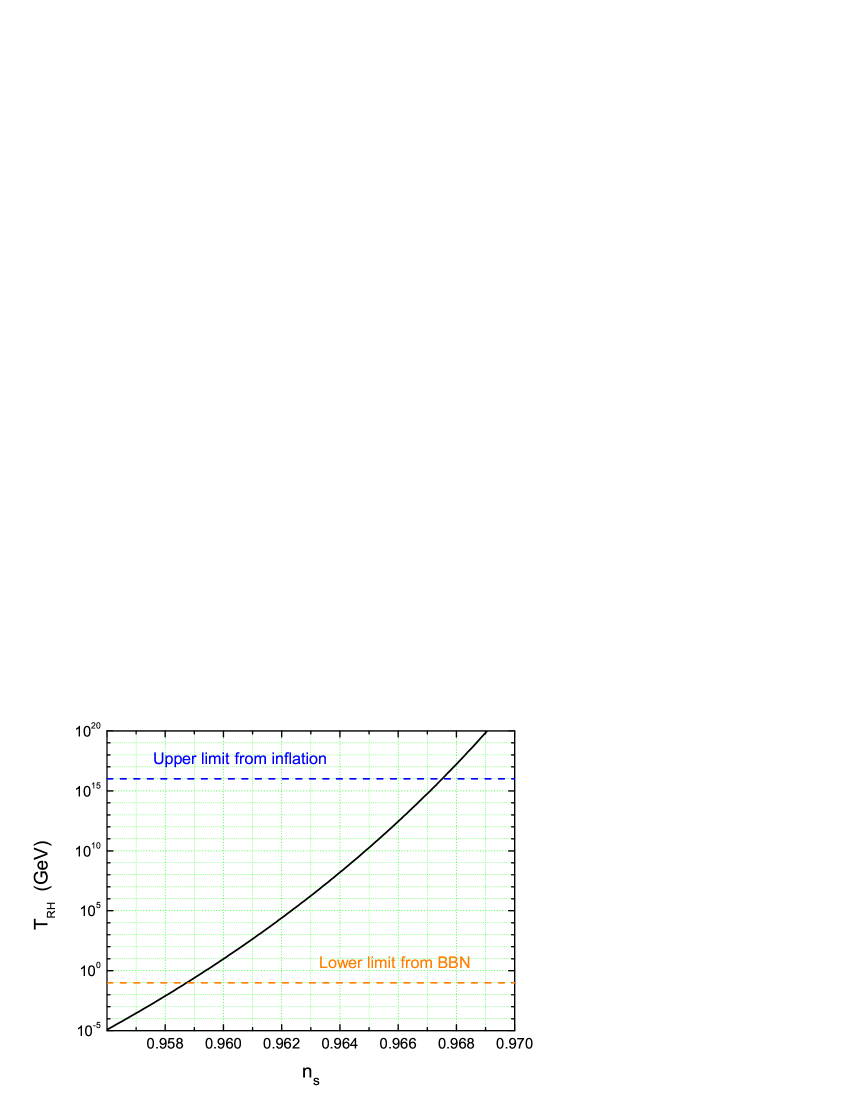
Figure 1: The reheating temperature $T_{\rm{RH}}$ as a function of the scalar spectral index $n_{s}$, where $\beta_{s}=1$ and $g_{\star s}=3.91$ are set.

From the bottom, the big bang nucleosynthesis (BBN) gives a constraint of the reheating temperature $T_{\rm{RH}}\gtrsim 10$ MeV hannestad . From the top, the constraint comes from the energy scale at the end of inflation $T_{\rm{RH}}\lesssim 10^{16}$ GeV. Under these constraints, one can see that the scalar spectral index should locate at the range of $0.959\lesssim n_{s}\lesssim 0.967$.

After the instantaneous reheating, the universe is filled with the relativistic plasma. We assume the expansion of the relativistic gas to be adiabatic, which is valid until the entropy transfer between the radiation and other components can be neglected. Therefore, the conservation of the entropy gives the increase of the scale factor from the reheating till the recombination Mielczarek ,

$$\frac{a_{rec}}{a(\tau_{s})}=\frac{T_{\rm{RH}}}{T_{rec}}\left(\frac{g_{\ast s}}{g_{\star s}}\right)^{1/3},$$ (9)

where $a_{rec}$ and $T_{rec}$ stand for the scale factor and the temperature at the recombination, respectively. $g_{\ast s}$ counts the effective number of relativistic species contributing to the entropy during the reheating. In the standard model of elementary particles, one has $g_{\ast}=g_{\ast s}=106.75$ at the energy scale above $\sim 1$ TeV Yuki , where $g_{\ast}$ counts the effective number of relativistic species contributing to the energy density during the reheating. Moreover, as pointed in Mielczarek , if the temperature of reheating is greater than the electroweak energy scale, $T_{\rm{RH}}\gtrsim 300$ GeV, one may expect that $g_{\ast}\geq 106.75$. Thus, in this paper we set $g_{\ast}=g_{\ast s}=106.75$. Based on Eq. (9), one easily obtain

$$\zeta_{s}=\frac{a(\tau_{2})}{a_{rec}}\frac{a_{rec}}{a(\tau_{s})}=\frac{T_{\rm{RH}}}{T_{CMB}(1+z_{eq})}\left(\frac{g_{\ast s}}{g_{\star s}}\right)^{1/3},$$ (10)

where we have used $T_{rec}=T_{CMB}(1+z_{rec})$. Finally, for the slow-roll inflation, the increase of the scale factor during the preheating stage with $\beta_{s}=1$ is given by Mielczarek

$$\zeta_{1}=\left(\frac{15m^{4}_{Pl}A_{s}(1-n_{s})^{2}}{64\pi^{2}g_{\ast}T_{\rm{RH}}^{4}}\right)^{1/3},$$ (11)

Even though $\zeta_{s}$ and $\zeta_{1}$ are dependent on $g_{\ast}$, $T_{\rm{RH}}$ is independent on $g_{\ast}$ as shown in Eq. (7). For WMAP Seven-year Mean, $n_{s}=0.967$, one has $\zeta_{s}\simeq 2.3\cdot 10^{24}$ and $\zeta_{1}\simeq 4.86$; while for WMAP Seven-year ML, $n_{s}=0.966$, one has $\zeta_{s}\simeq 1.11\cdot 10^{22}$ and $\zeta_{1}\simeq 6.07\cdot 10^{3}$. In the following, the resulting $\zeta_{s}$ and $\zeta_{1}$ under the frame of the slow-roll inflation will serve as referenced tools to obtain the solutions of the RGWs, even though some calculations of RGWs based on quantum normalization are free from the slow-roll inflation.

III RGWs in the accelerating universe

In the presence of the gravitational waves, the perturbed Robertson-Walker metric is given by

$$ds^{2}=a^{2}(\tau)[-d\tau^{2}+(\delta_{ij}+h_{ij})dx^{i}dx^{j}],$$ (12)

where the tensorial perturbation $h_{ij}$ is traceless $h^{i}_{\,\,i}=0$ and transverse $h_{ij,j}=0$. It can be decomposed into the Fourier $k$-modes and into the polarization states, denoted by $\sigma$, as

$$h_{ij}(\tau,{\bf x})=\sum_{\sigma=+,\times}\int\frac{d^{3}k}{(2\pi)^{3/2}}\epsilon^{(\sigma)}_{ij}h_{k}^{(\sigma)}(\tau)e^{i\bf{k}\cdot{x}},$$ (13)

where $h_{-k}^{(\sigma)*}(\tau)=h_{k}^{(\sigma)}(\tau)$ ensuring that $h_{ij}$ be real, the comoving wave number $k$ is related with the wave vector $\mathbf{k}$ by $k=(\delta_{ij}k^{i}k^{j})^{1/2}$, and the polarization tensor $\epsilon^{(\sigma)}_{ij}$ satisfies grishchuk :

$$\epsilon^{(\sigma)}_{ij}\epsilon^{(\sigma^{\prime}){ij}}=2\delta_{\sigma\sigma^{\prime}},\quad\epsilon^{(\sigma)}_{ij}\delta^{ij}=0,\quad\epsilon^{(\sigma)}_{ij}n^{j}=0,\quad\epsilon^{(\sigma)}_{ij}(-\mathbf{k})=\epsilon^{(\sigma)}_{ij}(\mathbf{k}).$$ (14)

In terms of the mode $h^{(\sigma)}_{k}$, the wave equation is

$$h^{(\sigma)}_{k}{{}^{\prime\prime}}(\tau)+2\frac{a^{\prime}(\tau)}{a(\tau)}h^{(\sigma)}_{k}{{}^{\prime}}(\tau)+k^{2}h^{(\sigma)}_{k}(\tau)=0,$$ (15)

where a prime means taking derivative with respect to $\tau$. The two polarizations of $h^{(\sigma)}_{k}(\tau)$ have the same statistical properties and give equal contributions to the unpolarized RGWs background, so the super index $(\sigma)$ can be dropped. Introducing a new notation grishchuk1 ; grishchuk ; zhang2 : $\mu_{k}(\tau)\equiv a(\tau)h_{k}(\tau)$, Eq.(15) reduces to

$$\mu_{k}^{\prime\prime}+\left(k^{2}-\frac{a^{\prime\prime}}{a}\right)\mu_{k}=0.$$ (16)

For the high-frequency limit, i.e., the term $a^{\prime\prime}/a$ can be neglected, the solution to Eq.(16) has the usual oscillatory from: $\mu_{k}(\tau)=A_{k}e^{-ik\tau}+B_{k}e^{ik\tau}$, where the constants $A_{k}$ and $B_{k}$ are determined by the initial conditions, and $h_{k}$ decreases adiabatically with the expansion of the universe:

$$h_{k}\propto\frac{e^{\pm ik\tau}}{a(\tau)}.$$ (17)

On the other hand, when the term $a^{\prime\prime}/a$ is dominant, the dominant solution of Eq.(16) is $\mu_{k}(\tau)=C_{k}a(\tau)$ for growing functions $a(\tau)$ in expanding universes, and

$$h_{k}=const.$$ (18)

In other words, when the wavelength of the mode $h_{k}(\tau)$, $\lambda={2\pi a}/{k}$, is much less than the horizon of the universe, $1/H=a^{2}(\tau)/a^{\prime}(\tau)$, $h_{k}(\tau)$ decays with the expansion of the universe; while if $\lambda\gg 1/H$, $h_{k}(\tau)$ will keep constant grishchuk ; grishchuk1 . The wavelengths of various modes $h_{k}$ are stretched outside the horizon during the inflation stage, and they will be constant until re-enter the horizon again. When the mode $h_{k}$ re-enters the horizon, it will decay as $h_{k}\propto 1/a(\tau)$.

The spectrum of RGWs $h(k,\tau)$ is defined by

$$\langle h^{ij}(\tau,\mathbf{x})h_{ij}(\tau,\mathbf{x})\rangle\equiv\int_{0}^{\infty}h^{2}(k,\tau)\frac{dk}{k},$$ (19)

where the angle brackets mean ensemble average. The dimensionless spectrum $h(k,\tau)$ relates to the mode $h_{k}(\tau)$ as TongZhang

$$h(k,\tau)=\frac{\sqrt{2}}{\pi}k^{3/2}|h_{k}(\tau)|.$$ (20)

The primordial spectrum of RGWs at the time $\tau_{i}$ of the horizon-crossing during the inflation has a power-law form grishchuk ; grishchuk3 ; zhang2 ; Miao :

$$h(k,\tau_{i})=A\left(\frac{k}{k_{H}}\right)^{2+\beta},$$ (21)

where the constant $A$ representing the initial condition is to be determined both from theories and observations. An exact de Sitter expansion, i.e., $\beta=-2$, yields a scale-invariant spectrum. Consider Eqs. (17), (18) and (20), one knows that the spectrum $h(k,\tau)$ will decay as $\propto 1/a(\tau)$ when it reenter the cosmic horizon, $1/H$. In the following, let us discuss the properties of the present RGWs spectrum $h(k,\tau_{0})$ with different frequency bands. The characteristic comoving wave number at a certain conformal time $\tau_{x}$ is give by

$$k_{x}\equiv k(\tau_{x})=\frac{2\pi a(\tau_{x})}{1/H(\tau_{x})}.$$ (22)

It is easily to obtain $k_{H}=2\pi\gamma$. Explicitly, one has following relations:

$$\frac{k_{E}}{k_{H}}=\zeta_{E}^{-\frac{1}{\gamma}},\quad\frac{k_{2}}{k_{E}}=\zeta_{2}^{\frac{1}{2}},\quad\frac{k_{s}}{k_{2}}=\zeta_{s},\quad\frac{k_{1}}{k_{s}}=\zeta_{1}^{\frac{1}{1+\beta_{s}}}.$$ (23)

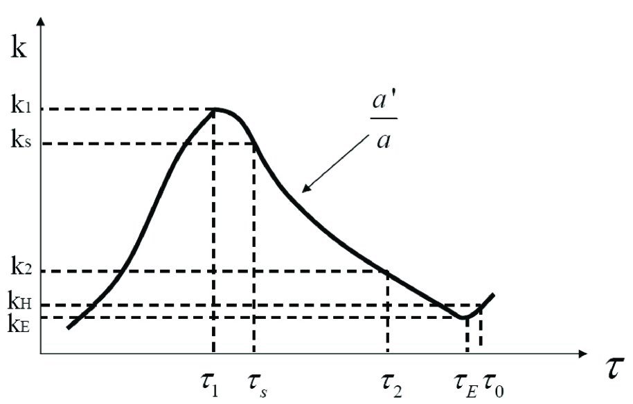
Figure 2: The evolution of $a^{\prime}/a.$

As shown in Fig.2, for the comoving wave number $k<k_{E}$, the modes of RGWs have been outside the horizon all the time. Thus, these modes never decay and keep their original amplitudes at present. For, $k_{E}<k<k_{H}$, the modes entered the horizon before the beginning of the acceleration and went out the horizon again before the present time. We denote the time of the mode $k$ entering and going out of the horizon as $\tau_{\ast}$ and $\tau_{\ast\ast}$, respectively. The corresponding scale factor are marked as $a_{\ast}$ and $a_{\ast\ast}$, respectively. Then, the present spectrum for $k_{E}<k<k_{H}$ can be written as

$$h(k,\tau_{0})=A\left(\frac{k}{k_{H}}\right)^{2+\beta}\frac{a_{\ast}}{a_{\ast\ast}}$$ (24)

According to Eqs.(5), (6) and (22), one can easily obtain $a_{\ast}/a(\tau_{E})=(k_{E}/k)^{2}$ and $a(\tau_{E})/a_{\ast\ast}=(k/k_{E})^{-\gamma}$, which lead to $h(k,\tau_{0})=h(k,\tau_{i})(k/k_{E})^{-(2+\gamma)}$. For $k>k_{H}$, after the modes entering the horizon, they have been inside the horizon up to now. Therefore, the spectrum for all the modes of $k>k_{H}$ has the following form:

$$h(k,\tau_{0})=A\left(\frac{k}{k_{H}}\right)^{2+\beta}\frac{a_{\ast}}{a(\tau_{0})},$$ (25)

where we have still used the notes $a_{\ast}$ standing for the scale factor when the $k-$mode enters the horizon. Using the similar analysis given above, one can get the present spectrum $h(k,\tau_{0})$ for different bands of wave number which correspond to different stages of the universe. Generally, we summarize the approximate solutions of $h(k,\tau_{0})$ uniformly as follows ,

$$h(k,\tau_{0})=A\left(\frac{k}{k_{H}}\right)^{2+\beta},\qquad k\leq k_{E};$$ (26)

$$h(k,\tau_{0})=A\left(\frac{k}{k_{H}}\right)^{\beta-\gamma}(1+z_{E})^{-\frac{2+\gamma}{\gamma}},\qquad k_{E}\leq k\leq k_{H};$$ (27)

$$h(k,\tau_{0})=A\left(\frac{k}{k_{H}}\right)^{\beta}(1+z_{E})^{-\frac{2+\gamma}{\gamma}},\qquad k_{H}\leq k\leq k_{2};$$ (28)

$$h(k,\tau_{0})=A\left(\frac{k}{k_{H}}\right)^{1+\beta}\left(\frac{k_{H}}{k_{2}}\right)(1+z_{E})^{-\frac{2+\gamma}{\gamma}},\qquad k_{2}\leq k\leq k_{s};$$ (29)

$$h(k,\tau_{0})=A\left(\frac{k}{k_{H}}\right)^{1+\beta-\beta_{s}}\left(\frac{k_{s}}{k_{H}}\right)^{\beta_{s}}\left(\frac{k_{H}}{k_{2}}\right)(1+z_{E})^{-\frac{2+\gamma}{\gamma}},\qquad k_{s}\leq k\leq k_{1}.$$ (30)

The factor $(1+z_{E})^{-\frac{2+\gamma}{\gamma}}$ means a reduction due to the accelerating expansion of the universe. The above equations reduce to the corresponding results shown in zhang2 , where $\gamma=1$ was assumed.

Another important quantity often used in constraining RGWs is its present energy density parameter defined by $\Omega_{GW}=<\rho_{g}>/{\rho_{c}}$, where $\rho_{g}=\frac{1}{32\pi G}h_{ij,0}h^{ij}_{,0}$ is the energy density of RGWs, and $\rho_{c}=3H_{0}^{2}/8\pi G$ is the critical energy density. A direct calculation yields grishchuk3 ; Maggiore

$$\Omega_{GW}=\int_{f_{low}}^{f_{upper}}\Omega_{g}(f)\frac{df}{f},$$ (31)

with

$$\Omega_{g}(f)=\frac{2\pi^{2}}{3}h^{2}_{c}(f)\Big{(}\frac{f}{H_{0}}\Big{)}^{2}$$ (32)

being the dimensionless energy density spectrum. We have used a new notation, $h_{c}(f)=h(f,\tau_{0})/\sqrt{2}$, called characteristic strain spectrum Maggiore or chirp amplitude Boyle . The lower and upper limit of integration in Eq.(31) can be taken to be $f_{low}\simeq f_{E}$ and $f_{upper}\simeq f_{1}$, respectively, since only the wavelength of the modes inside the horizon contribute to the total energy density.

In the present universe, the physical frequency relates to a comoving wave number $k$ as

$$f=\frac{k}{2\pi a(\tau_{0})}=\frac{k}{2\pi l_{H}}.$$ (33)

Thus, from Eqs. (23) and (33) one can easily get the each characteristic physical frequency: $f_{H}=H_{0}\simeq 2.28\cdot 10^{-18}$ Hz, $f_{E}\simeq 1.93\cdot 10^{-18}$ Hz, $f_{2}\simeq 9.3\cdot 10^{-17}$ Hz. Moreover, $f_{s}\simeq 2.14\cdot 10^{8}$ Hz and $f_{1}\simeq 4.71\cdot 10^{8}$ Hz for $n_{s}=0.967$; $f_{s}\simeq 1.03\cdot 10^{6}$ Hz and $f_{1}\simeq 8.04\cdot 10^{7}$ Hz for $n_{s}=0.966$. The values of $f_{1}$ are below the constraint from the rate of the primordial nucleosynthesis, $f_{1}\lesssim 3\times 10^{10}$ Hz grishchuk . When the acceleration epoch is considered, the constraint becomes $f_{1}\simeq 4\times 10^{10}$ Hz. Note that, Eq. (23) implies that $f_{1}$ depends on the value of $\beta_{s}$ but not $\beta$. Therefore, $f_{1}$ is a fixed value once $\beta_{s}$ has been chosen.

IV Observational constraints and the detection

As well known, the anisotropies and polarizations of CMB are contributed by two parts: tensor metric perturbations (gravitational waves) and curvature perturbations. Moreover, the B-mode CMB polarization is only produced by tensor perturbations. In literatures Peiris ; Spergel ; Hinshaw ; Komatsu , the tensor-to-scalar ratio $r$ is often introduced

$$r=\frac{\Delta^{2}_{h}(k_{0})}{\Delta^{2}_{\mathcal{R}}(k_{0})},$$ (34)

where $\Delta^{2}_{h}(k_{0})$ and $\Delta^{2}_{\mathcal{R}}(k_{0})$ are the power spectrum of the tensor perturbations and curvature perturbations evaluated at the pivot wavenumber $k^{p}_{0}=k_{0}/a(\tau_{0})=0.002$ Mpc^-1 Komatsu , respectively. The corresponding physical frequency is $f_{0}\simeq 3.09\times 10^{-18}$ Hz. For tensor power spectrum, one has the definition:

$$\Delta^{2}_{h}(k)\equiv h^{2}(k,\tau_{0}).$$ (35)

Hence, the non-zero value of $r$ implies the existence of gravitational wave background, and would be probed with measurements of the B-mode CMB polarization Amarie . Even though there is still no direct observation of $\Delta^{2}_{h}(k_{0})$, $\Delta^{2}_{\mathcal{R}}(k_{0})$ can be fixed by CMB observations, $\Delta^{2}_{\mathcal{R}}(k_{0})\equiv A_{s}=(2.43\pm 0.11)\cdot 10^{-9}$ by WMAP 7 Mean Komatsu . On the other hand, at present only observational constraints on $r$ have been given by WMAP Komatsu ; Hinshaw . The upper bounds of $r$ are recently constrained Komatsu as $r<0.24$ by WMAP+BAO+$H_{0}$ and $r<0.36$ by WMAP 7 only for the vanishing scalar running spectral index $\alpha_{s}$, and $r<0.49$ for the non-vanishing $\alpha_{s}$ by both the combination of WMAP+BAO+$H_{0}$ and the WMAP 7 only, respectively. Furthermore, using a discrete, model-independent measure of the degree of fine-tuning required, if $0.95\lesssim n_{s}<0.98$, in accord with current measurements, the tensor-to-ratio satisfies $r\gtrsim 10^{-2}$ Boyle2 . Therefore, one can normalize the RGWs at $k=k_{0}$ using Eq. (34), if $r$ can be determined definitely.

Since $k_{H}\leq k_{0}\leq k_{2}$, $h(k_{0},\tau_{0})$ re-entered the horizon during the matter domination and is now inside the present horizon. Therefore, $h(k_{0},\tau_{0})$ suffered a decay $\propto 1/a$ from the horizon re-entry to the present time. According to Eq. (28) one has

$$h(k_{0},\tau_{0})\equiv\Delta_{h}(k_{0})=A\left(\frac{k_{0}}{k_{H}}\right)^{\beta}(1+z_{E})^{-\frac{2+\gamma}{\gamma}}.$$ (36)

Therefore, $A$ can be fixed for a determined value of $\Delta_{h}(k_{0})$, given a definite value of $\beta$. Note that, the “thin-horizon” approximation that treats horizon re-entry as a “sudden” or instantaneous event Boyle has been used in Eq.(36). Thus, Eq.(36) is a normalization of RGWs provided by the observations of CMB. On the other hand, from the point of view of theories, the initial condition of RGWs could also be given, or some indirect connections between different parameters would exist. In the following, we discuss two different theories.

Firstly, the constant $A$ appearing in Eq. (21) can be determined by quantum normalization grishchuk :

$$A=b8\sqrt{\pi}\frac{l_{Pl}}{l_{0}},$$ (37)

where $b\equiv\gamma^{2+\beta}/|1+\beta|^{1+\beta}$ in our notation, $l_{Pl}=\sqrt{G}$ is the Plank length, and $l_{0}$ has been fixed to be Miao

$$l_{0}=bH_{0}^{-1}\zeta_{1}^{\frac{\beta-\beta_{s}}{1+\beta_{s}}}\zeta_{s}^{\beta}\zeta_{2}^{\frac{\beta-1}{2}}\zeta_{E}^{-(1+\frac{1+\beta}{\gamma})},$$ (38)

using the continuous conditions of $a(\tau)$ and $a^{\prime}(\tau)$ at the joining moments between two different phases. Here, it should be point out that the values of $\zeta_{s}$ and $\zeta_{1}$ shown in Eq. (38) will be chosen tentatively as those determined by Eqs. (10) and (11), respectively, since they are not known well. With the help of Eqs. (34), (37) and (38), Eq. (36) reduces to

$$\Delta_{\mathcal{R}}(k_{0})r^{1/2}=8\sqrt{\pi}l_{Pl}H_{0}\zeta_{1}^{\frac{\beta_{s}-\beta}{1+\beta_{s}}}\zeta_{s}^{-\beta}\zeta_{2}^{\frac{1-\beta}{2}}\zeta_{E}^{\frac{\beta-1}{\gamma}}\left(\frac{k_{0}}{k_{H}}\right)^{\beta},$$ (39)

which implies a relationship between $\beta$, $\beta_{s}$ and $r$. Given $\beta_{s}=1$, we illustrate $r$ as a function of $\beta$ in the left panel of Fig. 3 for $n_{s}=0.967$, $0.966$ and $0.963$, respectively. Here we plus the case of $n_{s}=0.963$ for comparison. One can see that the $r-\beta$ curves are almost overlap for $\beta\gtrsim-2$ and only small discrepancies exist for lower $\beta$. Taking $n_{s}=0.966$ for example, the constraints $r<0.49$, $r<0.36$ and $r<0.24$ lead to $\beta\gtrsim-2.038$, $\beta\gtrsim-2.035$, and $\beta\gtrsim-2.032$, respectively, while $r>0.01$ gives $\beta\lesssim-2.005$. Note that, these results are based on the validity of quantum normalization Eq. (37), however, it is not the unique initial condition. This is a manifestation of the vacuum ambiguity that is responsible for particle production in cosmological spacetimes Birrell . Furthermore, we have taken the values of $\zeta_{s}$ and $\zeta_{1}$ evaluated by using the slow-roll inflation model with a scalar potential $V(\phi)=\frac{1}{2}m^{2}\phi^{2}$ Mielczarek . If other different values of $\zeta_{s}$ and $\zeta_{1}$ are chosen, we find that the curves plotted in Fig. 3 will change sensitively. For simplicity, in this paper we will not consider these cases.

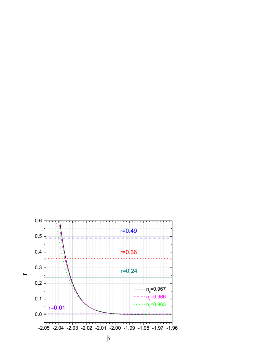
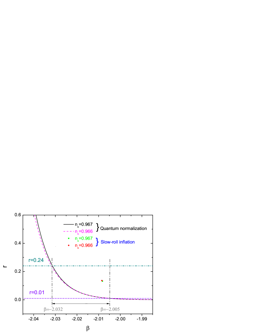
Figure 3: The relation between $r$ and $\beta$. Left: Three $r-\beta$ curves based on the quantum normalization for three different values of the scalar spectral index $n_{s}=0.967$, $n_{s}=0.966$ and $n_{s}=0.963$, respectively. Right: The comparison between the $r-\beta$ relations based on the quantum normalization and those based on the slow-roll inflation.

Secondly, from the point of view of the slow-roll inflation model, there is a natural relation between $n_{s}$ and $r$. For $V(\phi)=\frac{1}{2}m^{2}\phi^{2}$, using Eq. (8) one easily has $\epsilon=\eta$ and

$$n_{s}\approx 1-4\epsilon.$$ (40)

On the other hand, under the slow-roll approximation, the primordial tensor power spectrum and the primordial scalar power spectrum are respectively given as Boyle ; Kuroyanagi :

$$\Delta_{h}^{2}(k,\tau_{\ast})\approx\frac{16}{\pi}\left(\frac{H_{\ast}}{m_{\rm{Pl}}}\right)^{2},$$ (41)

$$\Delta_{\mathcal{R}}^{2}(k,\tau_{\ast})\approx\frac{1}{\pi\epsilon}\left(\frac{H_{\ast}}{m_{\rm{Pl}}}\right)^{2},$$ (42)

where $H_{\ast}$ is the Hubble rate during the inflation stage and is invariable for the slow-roll approximation. $\tau_{\ast}$ stands for the moment when the $k$-mode exits the horizon. According to the original definition of $r$, i.e., the ratio of the primordial tensor power spectrum to the primordial scalar power spectrum, one has Boyle ; Kuroyanagi

$$r\equiv\Delta_{h}^{2}(k,\tau_{\ast})/\Delta_{\mathcal{R}}^{2}(k,\tau_{\ast})=16\epsilon,$$ (43)

with the help of Eqs. (41) and (42). Note that the definition of $r$ in Eq.(43) is little different from that in Eq. (34). We will discuss the difference below. In the literatures of WMAP Peiris ; Spergel ; Komatsu , the primordial power spectrum are often written as

$$\Delta_{h}^{2}(k)=\Delta_{h}^{2}(k_{0})\left(\frac{k}{k_{0}}\right)^{n_{t}},$$ (44)

$$\Delta_{\mathcal{R}}^{2}(k)=\Delta_{\mathcal{R}}^{2}(k_{0})\left(\frac{k}{k_{0}}\right)^{n_{s}-1},$$ (45)

where $n_{t}$ is the tensorial spectral index. Generally, $n_{t}$ is $k-$depedent grishchuk91 ; Kosowsky ; LiddleA ; TongZhang , however, for simplicity we just consider $n_{t}$ as a constant in this paper. With the help of Eq. (21), one easily find that $n_{t}=2\beta+4$. Strictly speaking, based on Eq. (26), Eq. (44) is valid approximately since the mode $k=k_{0}$ has re-entered the horizon at the present time. An analogous case would also exist in Eq. (45), which was used to evaluate the reheating temperature in Mielczarek . However, as a conservative consideration, Eqs. (44) and (45) provide a good approximation to evaluate $r$. Now let us estimate the discrepancy between Eq. (34) and (43) in the following. From Eq. (44), it is straight forward to get $r\equiv\frac{\Delta_{h}^{2}(k_{E})}{\Delta_{\mathcal{R}}^{2}(k_{E})}=\frac{\Delta_{h}^{2}(k_{0})}{\Delta_{\mathcal{R}}^{2}(k_{0})}(k_{E}/k_{0})^{n_{t}+1-n_{s}}$. The differential factor $(k_{E}/k_{0})^{n_{t}+1-n_{s}}\sim 0.992$ for $n_{s}=0.966$ or $n_{s}=0.967$, where we have used Eq. (40) and the well known relation

$$n_{t}\approx-2\epsilon$$ (46)

in the slow-roll inflation. Allowing for the relation $n_{t}=2\beta+4$, the combination of Eqs. (43) and (46) give

$$r=-8n_{t}=-16(\beta+2).$$ (47)

This general linear relation is plotted in the right panel of Fig. 3. For a fixed value of $n_{s}$, $r$ can be determined through Eqs. (40) and (43), and then $\beta$ can also be determined through Eq. (47) correspondingly. We employ a red circle and a green square to stand for the values of $(\beta,r)=(-2.009,0.136)$ and $(\beta,r)=(-2.008,0.132)$ corresponding to the observations $n_{s}=0.966$ and $n_{s}=0.967$, respectively. For comparison, the relation between $r$ and $\beta$ determined by the quantum normalization was shown again, and the constraint of $0.01<r<0.24$ discussed above leads to $\beta$ localizing in the range of $-2.032<\beta<-2.005$. On the other hand, according to Eq. (47), the constraint of $0.01<r<0.24$ forces $\beta$ to lie in the range of $-2.015<\beta<-2.001$. Hence, under the condition $r\gtrsim 0.01$, $\beta$ has a tilt smaller than $-2$ both for the two theoretical bases. In fact, Eq. (47) directly implies $\beta<-2$ due to the definition of $r$ being positive.

In the following, we demonstrate the properties of the energy spectra of RGWs taking some definite values of $r$ and $\beta$ for example. Firstly, setting $n_{s}=0.966$, the approximate energy spectra with three different tensor-to-scalar ratios $r=0.49$, $r=0.01$ and $r=0.001$, which correspond to $\beta=-2.038$, $\beta=-2.005$ and $\beta=-1.985$ according to quantum normalization, respectively, are illustrated in the left panel of Fig. 4. It can be found that all the three cases of energy spectrum have the same amplitudes at $f=f_{1}\simeq 8.04\cdot 10^{7}$ Hz. This is a natural result from the quantum normalization. Plugging Eq. (37) into Eq. (30) with the help of Eqs. (23) and (38), one obtain

$$h_{c}(f_{1})=4\sqrt{2\pi}f_{1}l_{Pl},$$ (48)

and it is straight forward to obtain

$$\Omega_{g}(f_{1})=\frac{64\pi^{3}f_{1}^{4}l_{Pl}^{2}}{3H_{0}^{2}},$$ (49)

according to Eq. (32). We can see that $h_{c}(f_{1})$ and $\Omega_{g}(f_{1})$ are fixed values independent on $\beta$, since $f_{1}$ is independent on $\beta$. On the other hand, as shown in Fig. 4, a smaller $\beta$ leads to larger energy spectrum especially at lower frequencies. This property is contrary to that illustrated in Refs. Miao ; TongZhang ; zhangtong , where a fixed $\beta_{s}$ was chosen but the quantum normalization was not employed. Secondly, let us see the differences between the energy spectra of RGWs based on the quantum normalization and those based on the slow-roll inflation. In the right panel of Fig. 4, we plot the energy spectra of RGWs based on the two different theories for $n_{s}=0.966$ and $n_{s}=0.967$, respectively. For the slow-roll inflation, once $n_{s}$ is given, $r$ and $\beta$ will be determined subsequently. Concretely, as analyzed above, $n_{s}=0.966$ and $n_{s}=0.967$ correspond to $r=0.136$ and $r=0.132$, respectively. For comparison, we also choose the same values of $r$ in the energy spectra based on quantum normalization, and moreover, it is easy to have $\beta\simeq-2.027$ for $r=0.136$ or $r=0.132$ using Eq. (39). As shown in the right panel of Fig. 4, the energy spectra of RGWs based on these two theories are almost the same at $f\leq f_{2}$ both for $n_{s}=0.966$ and $n_{s}=0.967$. This is because of the normalization from the CMB observations at $f=f_{0}$, where $\Omega_{g}(f)/r$ is a fixed value. Therefore, around $f=f_{0}$, $\Omega_{g}(f)$ depends on $r$ sensitively rather than $\beta$, since $\Omega_{g}(f)$ depends on $\beta$ in the way of $\Omega(f)\propto(f/f_{0})^{2\beta}$. Let us take $\Omega_{g}(f_{2})$ for example. With the help of Eqs. (28), (32) and (36), one can easily derive that $\Omega_{g}(f_{2})\propto r(\frac{f_{2}}{f_{0}})^{2\beta}(\frac{f_{2}}{H_{0}})^{2}$. Among the four curves illustrated in the right panel of Fig.4, the biggest relative discrepancy of $\Omega_{g}(f_{2})$, existing between the sets $(r=0.136,\beta=-2.008)$ and $(r=0.132,\beta=-2.027)$, is about $17\%$. Similarly, for the modes which re-entered the horizon during radiation domination, one has $\Omega_{g}(f)\propto r(\frac{f}{f_{0}})^{2\beta}(\frac{f}{H_{0}})^{4}$ due to Eq. (29). Therefore, for fixed $r$, the discrepancies of the energy spectra based on quantum normalization and those based on slow-roll inflation are larger and larger with the increasing frequency, since a difference $\Delta\beta\simeq 0.02$ in the indices between them always exists. In the very high frequency band $f_{s}<f<f_{1}$, not only the discrepancy discussed above is larger, but also the energy spectra manifest different properties for different values of $n_{s}$. The latter phenomenon results from that $n_{s}=0.966$ and $n_{s}=0.967$ lead to different values of $f_{s}$ and $f_{1}$ as analyzed below Eq. (33), either on the basis of quantum normalization or slow-roll inflation. The value of $f_{s}$ depends on $n_{s}$ very sensitively, while $f_{1}$ depends on $n_{s}$ much less sensitively compared to $f_{s}$. These properties would become an effective tool to discriminate the value of $n_{s}$, and could be an interesting object of the high-frequency gravitational wave detectors cruise ; fangyu ; Akutsu .

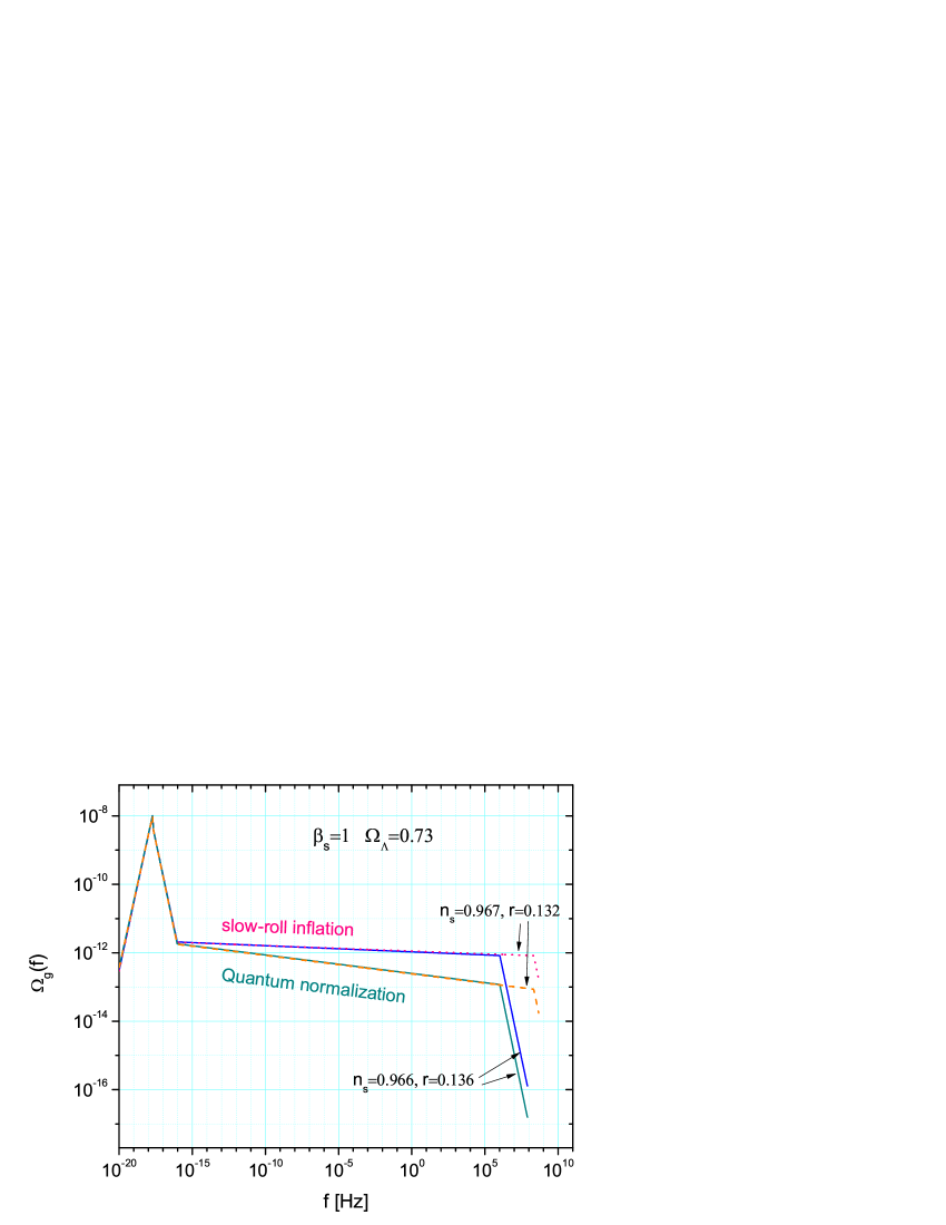
Figure 4: Left: The energy density spectra of RGWs based on the quantum normalization with $r=0.49(\beta=-2.038)$, $r=0.01(\beta=-2.005)$ and $r=0.001(\beta=-1.985)$, respectively, for $n_{s}=0.966$. Right: The comparisons between the energy density spectra based on the quantum normalization and the slow-roll inflation for $n_{s}=0.966$ and $n_{s}=0.967$, respectively.

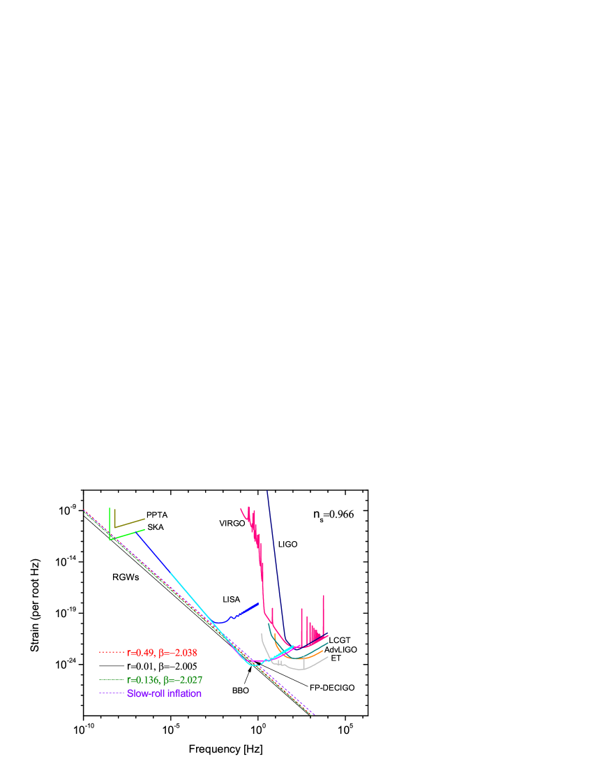
Figure 5: The strain of RGWs with different parameters for $n_{s}=0.966$ confronts against the current and planed GW detectors. The sensitivity curves of PPTA and SKA using pulsar timing technique are taken from Refs.Jenet and Sesana , respectively. The curve of BBO is generated using the online “Sensitivity curve generator” lisa with the parameters in Table II of Ref.Crowder and Table I of Ref.Cutler . The curve of FP-DECIGO is taken from Ref.Kawamura . The sensitivity curves of the ground-based interferometers AdvLIGO, LCGT and ET are taken from Refs.advligo , lcgt and Hild , respectively.

Below, let us discuss the detection of RGWs using the ongoing and planed gravitational detectors which are sensitive at different frequency bands. As shown in the right panel of Fig. 4, there is nearly no difference between the RGWs with $n_{s}=0.966$ and those with $n_{s}=0.967$ at $f<f_{s}$, both based on quantum normalization and slow-roll inflation. Thus, we just take $n_{s}=0.966$ for demonstration in the following. As a conservative evaluation, in Fig. 5 we show the strain sensitivity curves of various gravitational wave detectors and the strain amplitudes, $h_{c}(f)/\sqrt{f}$, of the RGWs for $n_{s}=0.966$ based on quantum normalization and slow-roll inflation, respectively. These detectors contain the PPTA Jenet and SKA Sesana using the pulsar timing technique, the space-based laser interferometers such as LISA lisa , BBO Crowder ; Cutler , and the Fabry-Perot DECIGO Kawamura , the ground-based laser interferometers including the first generation LIGO ligo1 and VIRGO virgocurve , the second generation AdvLIGO advligo and LCGT lcgt , and the third generation ET Hild . One can see that all the ground-based interferometers can hardly detect the theoretical RGWs discussed above. PPTA and LISA also have difficulties to catch RGWs, however, the planed SKA, BBO and DECIGO are promising to detect RGWs since they have relative higher sensitivities. In order to show the detectabilities of RGWs by SKA and DECIGO/BBO more clearly, we enlarge the two parts of SKA and DECIGO/BBO which are shown in Fig. 6. As can be seen in the left panel of Fig. 6, around the frequencies $3-5\times 10^{-9}$ Hz, the spectra of RGWs with different parameters of $r$ (and in turn the different corresponding $\beta$ due to the $r-\beta$ relation) based on quantum normalization have different amplitudes, and they are promising to be distinguished by SKA. However, the spectrum based on slow-roll inflation is hardly distinguished from that based on quantum normalization with $r=0.49(\beta=-2.038)$ by SKA, since two lines almost overlap in the frequency response band of SKA. On the other hand, in the right panel of Fig. 6 one can see that, RGWs based on slow-roll inflation are easier to be distinguished from those based on quantum normalization by DECIGO or BBO in the frequency range $\sim 10^{-2}-10^{0}$ Hz. Furthermore, since DECIGO/BBO has a wider frequency response band in contrast to SKA, the $r-\beta$ has the potential to be examined. In conclusion, the combination of SKA and DECIGO/BBO provides an important tool not only distinguishing different theoretical models of RGWs but also determining the corresponding parameters.

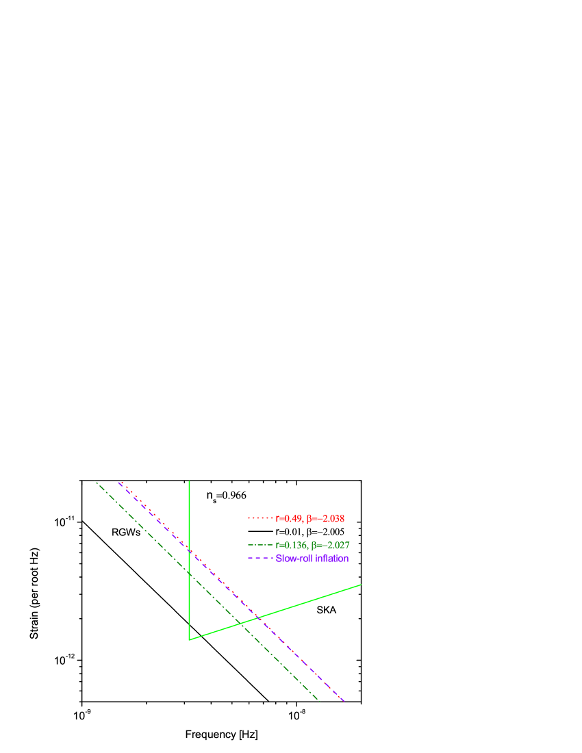
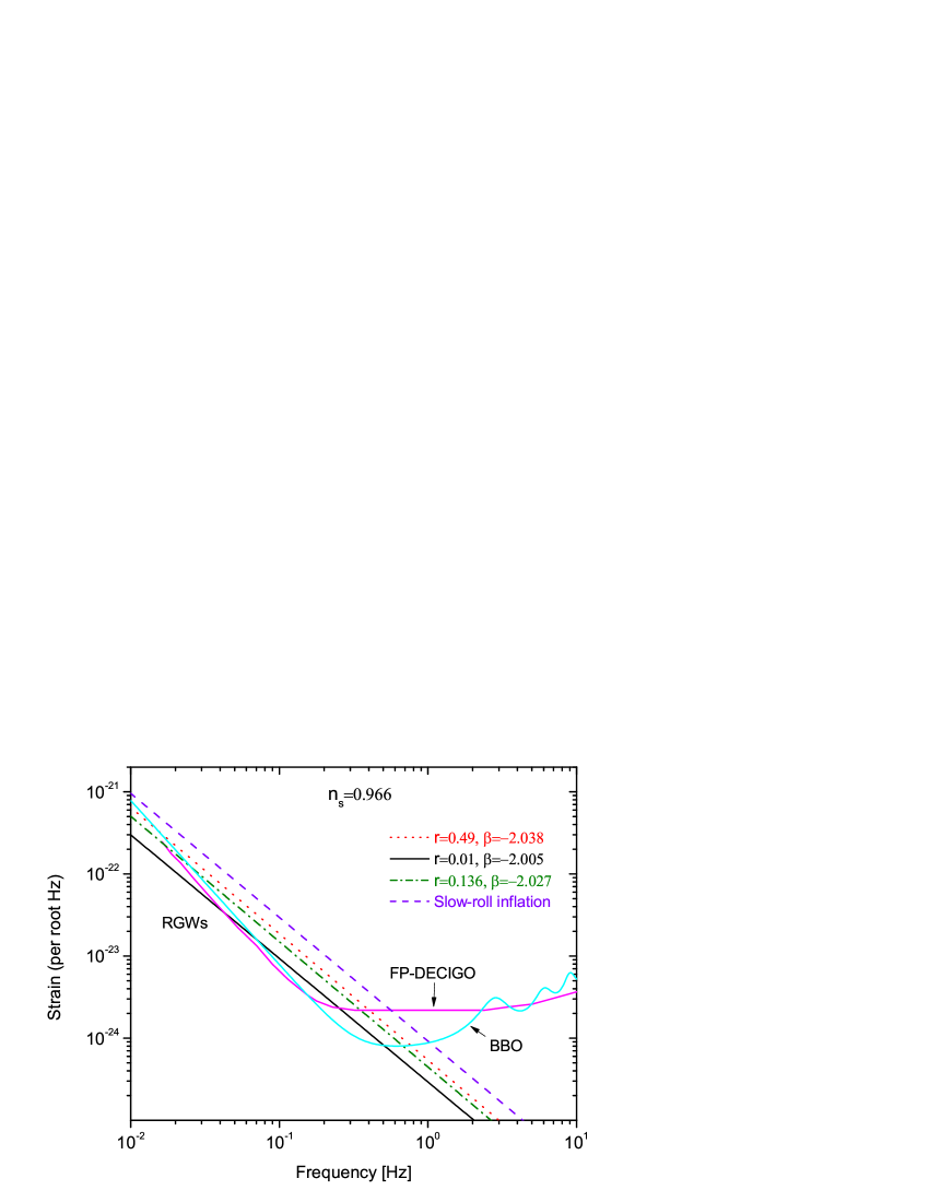
Figure 6: A zoom plot of the two parts of SKA and FP-DCIGO/BBO. All the values of parameters in RGW models and the sensitivity curves of the three gravitational wave detectors are exactly the same as those shown in Fig. 5.

V Discussions

We determined the expansion histories of the preheating stage and the radiation-dominated stage due to the the reheating temperature which is recalculated using the latest observations of WAMP 7-year. Based on that, we illustrated the approximate solutions of RGWs in the current accelerating stage for various frequency bands. We found that the frequency $f_{s}$, describing that the mode re-entered the horizon at the moment of the reheating, is dependent on $n_{s}$ sensitively, however, the upper limit frequency of RGWs depends on the value of $n_{s}$ much less sensitively. Combing the quantum normalization of RGWs with the CMB observations, we obtained a relation between the tensor-to-scalar ratio $r$ and the inflation index $\beta$ for the fixed preheating index $\beta_{s}=1$. According to the relation between $r$ and $\beta$ with a fixed $n_{s}=0.966$, we find that a relatively tight constraint $0.01<r<0.24$ leads to $\beta$ localizing in a range of $-2.032<\beta<-2.005$ based on quantum normalization and in a more narrow range of $-2.015<\beta<-2.001$ based on slow-roll inflation, respectively. We plotted the spectrum and the energy density spectrum of the RGWs for three cases of $r=0.49(\beta=-2.038)$, $r=0.01(\beta=-2.005)$, and $r=0.001(\beta=-1.985)$, respectively. It was found that a lager $r$, i.e., a smaller $\beta$ leads to a larger spectrum of RGWs especially at lower frequencies. For comparison, we also illustrated the spectra of RGWs with the parameters of $r$ and $\beta$ given by the slow-roll inflation. Concretely, for $n_{s}=0.966$, one has $r=0.136$ and $\beta=-2.009$, and for $n_{s}=0.967$, one has $r=0.132$ and $\beta=-2.008$. It was found that, for the same value of $r$, the discrepancy of the energy spectra based on quantum normalization and those based on slow-roll inflation is larger and larger with the increasing frequency. However, our analysis above does not not apply, in general, to less conventional models of inflation where the RGW spectrum and the observed spectrum of scalar perturbations are produced with different primordial mechanisms Bozza ; Gasperini , and, as a consequence, they are in principle completely decoupled.

Among the current and planed GW detectors, only the planed SKA using the pulsar timing technique, and the planed space-based interferometers BBO and DECIGO are promising to detect RGWs. However, these results are based on the referenced values of $\zeta_{1}$ and $\zeta_{s}$ which are obtained from the combination of CMB observations and the slow-roll inflation with a concrete potential $V(\phi)=\frac{1}{2}m^{2}\phi^{2}$. Note that, the values of $\zeta_{1}$ and $\zeta_{s}$ depend sensitively on the reheating temperature $T_{\rm{RH}}$ which is dependent on $n_{s}$ sensitively. However, the $r-\beta$ relation is nearly not dependent on $n_{s}$ once the form of the potential $V(\phi)=\frac{1}{2}m^{2}\phi^{2}$ is given. Hence, for the same value of $r$, different $n_{s}$ only affects the very high frequency RGWs that re-entered the horizon before the radiation-dominant stage. Therefore, to a certain extant, our analysis of the detection in the frequency range $f\leq 10^{3}$ Hz is general, even though the determination of the reheating temperature from CMB has very large uncertainties. As forecasted in Ref. Mielczarek , the future CMB experiments such as the Plank satellite Planck , the ground-based ACTPol Niemack and the planned CMBPol CMBpol will provide significant reductions of the uncertainties of the reheating temperature $T_{\rm{RH}}$. Therefore, one expect accordingly that the expansion histories of the very early universe would be known better. On the other hand, the values of $\zeta_{1}$ and $\zeta_{s}$ could be chosen independently on the slow-roll inflation scenario, which would be studied in the future work.

ACKNOWLEDGMENT: This work is supported by the National Science Foundation of China under Grant No. 11103024, and has been supported in part by the Fundamental Research Fund of Korea Astronomy and Space Science Institute.

References

- (1) L.P. Grishchuk, Sov.Phys.JETP 40, 409 (1975); Class.Quant.Grav.14, 1445 (1997).
- (2) L.P. Grishchuk, in Lecture Notes in Physics, Vol.562, p.167, Springer-Verlag, (2001), arXiv: gr-qc/0002035.
- (3) L.P. Grishchuk, arXiv: gr-qc/0707.3319.
- (4) A.A. Starobinsky, JEPT Lett. 30, 682 (1979); Sov. Astron. Lett. 11, 133 (1985); V.A. Rubakov, M. Sazhin, and A. Veryaskin, Phys. Lett. B 115, 189 (1982); R. Fabbri and M.D. Pollock, Phys. Lett. B 125, 445 (1983); L. F. Abbott and M.B. Wise, Nucl. Phys. B 244, 541 (1984); B. Allen, Phys. Rev. D 37, 2078 (1988); V. Sahni, Phys. Rev. D 42, 453 (1990); H. Tashiro, T. Chiba, and M. Sasaki, Class. Quant. Grav. 21, 1761 (2004); A. B. Henriques, Class. Quant. Grav. 21, 3057 (2004); W. Zhao and Y. Zhang, Phys. Rev. D 74, 043503 (2006).
- (5) M. Maggiore, Phys. Rept. 331, 283 (2000).
- (6) M. Giovannini, PMC Phys. A 4, 1 (2010).
- (7) Y. Zhang et al., Class. Quant. Grav. 22, 1383 (2005); Chin. Phys. Lett. 22, 1817 (2005);
- (8) Y. Zhang et al., Class. Quant. Grav.23, 3783 (2006).
- (9) http://www.ligo.caltech.edu/.
- (10) http://www.ligo.caltech.edu/advLIGO/.
- (11) S. J. Waldman (the LIGO Scientific Collaboration), arXiv:1103.2728.
- (12) A. Freise, et al., Class. Quant. Grav. 22, S869 (2005); http://www.virgo.infn.it/.
- (13) https://wwwcascina.virgo.infn.it/senscurve/.
- (14) B. Willke, et al., Class. Quant. Grav. 19, 1377 (2002); http://geo600.aei.mpg.de/; http://www.geo600.uni-hannover.de/geocurves/.
- (15) J. Degallaix, B. Slagmolen, C. Zhao, L. Ju and D. Blair, Gen. Relativ. Gravit. 37, 1581 (2005); P. Barriga, C. Zhao, and D.G. Blair, Gen. Relativ. Gravit. 37, 1609 (2005).
- (16) K. Kuroda and LCGT Collaboration, Class. Quantum Grav. 23, S215 (2006) .
- (17) M. Punturo et al., Class. Quantum Grav. 27, 194002 (2010).
- (18) S. Hild et al., Class. Quantum Grav. 28, 094013 (2011).
- (19) S.L. Larson, W.A. Hiscock, and R.W. Hellings, Phys. Rev. D, 62, 062001 (2000); S.L. Larson, R.W. Hellings, and W.A. Hiscock, Phys. Rev. D, 66, 062001 (2002).
- (20) http://www.srl.caltech.edu/~shane/sensitivity/.
- (21) J. Crowder and N.J. Cornish, Phys. Rev. D, 72, 083005 (2005).
- (22) C. Cutler and J. Harms, Phys. Rev. D, 73, 042001 (2006).
- (23) S. Kawamura et al., Class. Quantum Grav. 23, S125-S131 (2006); H. Kudoh, A. Taruya, T. Hiramatsu, and Y. Himemoto, Phys. Rev. D, 73, 064006 (2006).
- (24) G. Hobbs, Class. Quant. Grav. 25, 114032 (2008); J. Phys. Conf. Ser. 122, 012003 (2008); R.N. Manchester, AIP Conf. Series. Proc. 983, 584 (2008), arXiv:0710.5026; arXiv:1004.3602.
- (25) F.A. Jenet, et al., Astrophys. J. 653, 1571 (2006).
- (26) M. Kramer et al., New Astr. 48, 993 (2004); www.skatelescope.org.
- (27) A.M. Cruise, Class.Quant.Grav. 17, 2525 (2000) ; A.M. Cruise and R.M.J. Ingley, Class. Quant. Grav. 22, S479 (2005); Class. Quant. Grav. 23, 6185 (2006); M.L. Tong and Y. Zhang, Chin. J. Astron. Astrophys. 8, 314 (2008).
- (28) F.Y. Li, M.X. Tang and D.P. Shi, Phys. Rev. D 67, 104008 (2003); F.Y. Li et al., Eur. Phys. J. C 56, 407 (2008); M.L. Tong, Y. Zhang, and F.Y. Li, Phys. Rev. D 78, 024041 (2008).
- (29) T. Akutsu et al., Phys. Rev. Lett. 101, 101101 (2008).
- (30) M. Zaldarriaga and U. Seljak, Phys.Rev.D55, 1830 (1997); M. Kamionkowski, A. Kosowsky, and A. Stebbins, Phys. Rev. D55, 7368 (1997); B.G. Keating, P.T. Timbie, A. Polnarev, and J. Steinberger, Astrophys. J. 495, 580 (1998); J. R. Pritchard and M. Kamionkowski, Ann. Phys.(N.Y.) 318, 2 (2005); W. Zhao and Y. Zhang, Phys.Rev.D74, 083006 (2006); T.Y Xia and Y. Zhang, Phys. Rev. D78, 123005 (2008); Phys. Rev. D79, 083002 (2009); W. Zhao and D. Baskaran, Phys. Rev. D 79, 083003 (2009).
- (31) H.V. Peiris, et al, Astrophys. J. Suppl. 148, 213 (2003). D.N. Spergel, et al, Astrophys. J. Suppl. 148, 175 (2003).
- (32) D.N. Spergel, et al, Astrophys. J. Suppl. 170, 377 (2007). L. Page, et al, Astrophys.J.Suppl. 170, 335 (2007).
- (33) G. Hinshaw, et al, Astrophys. J. Suppl. 180, 225 (2009); J. Dunkley, et al, Astrophys. J. Suppl. 180, 306 (2009).
- (34) E. Komatsu, et al, Astrophys. J. Suppl. 192, 18 (2011).
- (35) Planck Collaboration, arXiv:astro-ph/0604069; http://www.rssd.esa.int/index.php?project=Planck.
- (36) M.D. Niemack et al., Proc. SPIE, 7741, 77411S (2010).
- (37) J. Dunkley et al., in CMBPol Mission Concept Study: Prospects for Polarized Foreground Removal, 1141, 222 (AIP, New York, 2009).
- (38) E.W. Kolb and M.S. Turner, The Early Universe, (Addison-Wesley, Reading, MA, 1990).
- (39) K. Nakayama, S. Saito, Y. Suwa, and J. Yokoyama, JCAP, 0806, 020 (2008).
- (40) J. Mielczarek, Phys. Rev. D 83, 023502 (2011).
- (41) Y. Zhang, M.L. Tong, and Z.W. Fu, Phys. Rev. D 81, 101501(R), (2010).
- (42) H. X. Miao and Y. Zhang, Phys. Rev. D 75, 104009 (2007).
- (43) Y. Watanabe and E. Komatsu, Phys. Rev. D 73, 123515 (2006).
- (44) Here, the superscript means“physical”, and we use standing for the conmoving number.
- (45) S. Kuroyanagi, T. Chiba, and N. Sugiyama, Phys. Rev. D 79, 103501 (2009).
- (46) M.S. Turner, Phys. Rev. D 28, 1243 (1983).
- (47) J. Martin and C. Ringeval, Phys. Rev. D 82, 023511 (2010).
- (48) A.A. Starobinsky, Phys. Lett. B 91, 99 (1980); S. Kuroyanagi, T. Chiba and N. Sugiyama, Phys. Rev. D 79, 103501 (2009).
- (49) A. R. Liddle and D. H. Lyth, Phys. Lett. B291, 391 (1992); Phys. Rep. 231, 1 (1993); Cosmological inflation and large-scale structure, Cambridge University Press (2000).
- (50) S. Hannestad, Phys. Rev. D 70, 043506 (2004); M. Kawasaki, K. Kohri and N. Sugiyama, Phys. Rev. D 62, 023506 (2000).
- (51) M.L. Tong, Y. Zhang, Phys. Rev. D 80, 084022 (2009).
- (52) L.A. Boyle and P.J. Steinhardt, Phys. Rev. D 77, 063504 (2008).
- (53) M. Amarie, C. Hirata and U. Seljak, Phys. Rev. D 72, 123006 (2005); A. Amblard, A. Cooray and M. Kaplinghat, Phys. Rev. D 75, 083508 (2007).
- (54) L.A. Boyle, P.J. Steinhardt, and N. Turok, Phys. Rev. Lett. 96, 111301 (2006).
- (55) N.D. Birrell and P.C.W. Davies, Quantum Fields in Curved Space (Cambridge University Press, Cambridge, England, 1982).
- (56) A. Kosowsky and M.S. Turner, Phys. Rev. D 52, R1739 (1995).
- (57) L.P. Grishchuk and M. Solokhin, Phys. Rev. D 43, 2566, (1991); W. Zhao, D. Baskaran, and L.P. Grishchuk, Phys. Rev. D 82, 043003 (2010).
- (58) A. Sesana, A. Vecchio, and C.N. Colacino, Mon. Not. R. Astron. Soc. 390, 192 (2008).
- (59) V. Bozza, M. Gasperini, M. Giovannini and G. Veneziano, Phys. Lett. B 543, 14 (2002).
- (60) M. Gasperini, M. Giovannini and G. Veneziano, Nucl. Phys. B 694, 206 (2004).