Steady Schrödinger cat state of a driven Ising chain

Abstract

For short-range interacting systems, no Schrödinger cat state can be stable when their environment is in thermal equilibrium. We show, by studying a chain of two-level systems with nearest-neighbour Ising interactions, that this is possible when the surroundings consists of two heat reservoirs at different temperatures, or of a heat reservoir and a monochromatic field. The asymptotic state of the considered system can be a pure superposition of mesoscopically distinct states, the all-spin-up and all-spin-down states, at low temperatures. The main feature of our model leading to this result is the fact that the Hamiltonian of the chain and the dominant part of its coupling to the environment obey the same symmetry.

1 Introduction

The apparent classical behavior of macroscopic objects is thought to find its origin in the unavoidable interaction of any system with its environment Z ; JZ . For example, non-classical correlations between quantum systems B ; W are expected to be fragile against this influence. This fragility of quantum entanglement is confirmed by studies showing that an initial entanglement between two independent open systems disappears in a finite time DH ; YE ; JJ . As a matter of fact, when several independent systems interact with an environment in thermal equilibrium, their state generically relaxes to their uncorrelated canonical thermal state. Consequently, even classical correlations are destroyed in this situation. This is not necessarily the case with a non-equilibrium surroundings. For an environment consisting simply of two heat reservoirs at different temperatures, the steady state of two non-interacting systems can be entangled EPJB2 . Thus, in this case, an initially uncorrelated state can evolve into a quantum-mechanically entangled one. General results have been obtained concerning the steady state of a Markovian master equation of Lindblad form K ; TV . Within this approach, any pure state can be asymptotically reached with a purely dissipative dynamics, but not all states are attainable if the environment influence is required to be local.

Probably the most amazing predictions of quantum theory arise when the superposition principle is applied to macroscopic objects. All states in the Hilbert space of any system can genuinely exist. There is no a priori restriction, even in the case, for instance, of the Earth’s center of mass. Quantum coherent superpositions of macroscopically distinguishable states were first discussed by E. Schrödinger who considered a cat in a dead-alive state S . Here also, environmental degrees of freedom are thought to play an essential role. Under their influence, such freak states would decay very quickly into statistical mixtures if they would happen to occur CL ; WM ; MNS ; PHPM . Recently, Schrödinger cat states have been realized experimentally as superpositions of motional wavepackets of trapped ions MMKW , microwave cavity coherent fields BH ; DDH , magnetic flux states of superconducting quantum interference devices FPCTL , internal states of trapped ions SM ; LW , photons polarizations ZCZYBP , nuclear spins states in benzene molecules LK , free-propagating light coherent states OTLG , polarization and spatial modes of photons GP . In all these experiments, the dissipative influence of the environment tends to destroy the created superposition of states and is one of the main obstacles to overcome to produce and observe it.

However, considering the positive impact on quantum entanglement of driving the environment out of equilibrium EPJB2 , one can wonder whether a Schrödinger cat state can be stable in a multiple-heat-reservoir surroundings or in the presence of a monochromatic field. We address this issue in this paper by studying a chain of two-level systems (TLS), with nearest-neighbour Ising interactions, coupled to a heat bath and a monochromatic field, as illustrated in Fig.1. Couplings between the TLS are necessary to obtain a steady Schrödinger cat state TV . It is proved below that, for any TLS system, its ground state cannot be a Schrödinger cat state when only short range interactions are present. Consequently, such a superposed state is necessarily unstable with an environment in thermal equilibrium. We will see that, on the contrary, if the surroundings includes a monochromatic field, or a second heat bath, the TLS steady state can be a pure superposition of mesoscopically distinct states, even if the interactions between the TLS are short-ranged.

The paper is organized as follows. The model we consider is presented in the next section. Section 3 is devoted to the study of the TLS Hamiltonian. In the following section, we derive equations that determine the asymptotic state of the TLS in the regime of weak coupling to both the heat reservoir and the monochromatic field. In section 5, we show that, when the field frequency is equal to a particular transition frequency of the TLS system, the TLS asymptotic state is, at low bath temperature, a steady multipartite entangled state that cannot be obtained at thermal equilibrium. Moreover, a TLS-field coupling strength regime can exist, where it is a pure Schrödinger cat state. In the last section, we summarize our results and mention some questions raised by our work. The case of a two-heat-reservoir environment is considered in the last Appendix.

2 Model

We consider a system consisting of $2N$ two-level systems, a heat bath and a monochromatic field, described by the Hamiltonian

$$H=H_{TLS}+\alpha^{-1}\epsilon_{f}\sigma^{x}_{N}(a^{\dagger}+a)+\omega a^{\dagger}a\\ +e\sum_{n=1}^{2N}\sigma^{x}_{n}\pi+\epsilon\sum_{n=1}^{2N}\left(\sigma^{x}_{n}\pi^{x}_{n}+\sigma^{y}_{n}\pi^{y}_{n}+\sigma^{z}_{n}\pi^{z}_{n}\right)+H_{\cal B},$$ (1)

where $\omega$ is the field frequency, $e$, $\epsilon\ll e$ and $\epsilon_{f}\ll e$ are energies characterizing the coupling strengths of the TLS to their environment, $\alpha$ is a dimensionless constant that will be defined below, $H_{\cal B}$ is the bath Hamiltonian, $\pi$ and $\pi^{\nu}_{n}$ where $\nu\in\{x,y,z\}$, are observables of the bath, and

$$H_{TLS}=-J\sum_{n=1}^{2N-1}\sigma^{z}_{n}\sigma^{z}_{n+1}-\sum_{n=1}^{N}h_{n}(\sigma^{z}_{n}-\sigma^{z}_{2N+1-n})$$ (2)

is the TLS Hamiltonian. The coupling constant $J>0$ and the fields $h_{n}$ are assumed to obey $h_{n}>0$ and $\sum_{n}h_{n}<J/2$. The annihilation operator $a$ satisfies the bosonic commutation relation $[a,a^{\dagger}]=1$. In the following, the notation ${\tilde{n}}$ is used for the eigenvalues of the number $a^{\dagger}a$. The Pauli operator $\sigma^{z}_{n}$ has eigenvalues $\pm 1$ and the corresponding eigenstates are denoted by $|\pm\rangle_{n}$. The observables $\sigma_{n}^{x}$ and $\sigma_{n}^{y}$ are then defined by $\sigma_{n}^{x}|\pm\rangle_{n}=|\mp\rangle_{n}$ and $\sigma_{n}^{y}=i\sigma_{n}^{x}\sigma_{n}^{z}$. The main assumption underlying our model is that the dominant contribution to the interaction between the TLS and their environment is a uniform coupling to the heat reservoir, of the form $\pi S_{x}$ where $S_{x}=\sum_{n}\sigma^{x}_{n}$. The term proportional to the energy $\epsilon$ in (1), describes the small deviation, which is assumed local and generic, of the TLS-bath interaction from this ideal form. The coupling to the monochromatic field can be generalized to $\alpha^{-1}\epsilon_{f}\sum_{n,\nu}\sigma^{\nu}_{n}(\lambda_{n\nu}a^{\dagger}+\lambda_{n\nu}^{*}a)$. Our main conclusions remain the same provided $\lambda_{Nx}-i\lambda_{Ny}-\lambda_{N+1x}-i\lambda_{N+1y}\neq 0$.

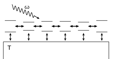
Figure 1: Schematic representation of a chain of two-level systems with nearest-neighbour interactions and coupled to a heat reservoir of temperature $T$ and to a monochromatic field of frequency $\omega$.

The initial state of the total system is

$$\Omega=\sum_{k,l}r_{kl}|k\rangle\langle l|\otimes Z^{-1}e^{-H_{\mathrm{\cal B}}/T}\otimes|\alpha\rangle\langle\alpha|,$$ (3)

where $k$ and $l$ run over the eigenstates of $H_{TLS}$, the density matrix elements $r_{kl}$ are arbitrary, $T$ is the temperature of the heat bath, $Z=\mathrm{Tr}\exp(-H_{\mathrm{\cal B}}/T)$, and $|\alpha\rangle$ is a coherent state of the field, i.e., $a|\alpha\rangle=\alpha|\alpha\rangle$. Throughout this paper, units are used in which $\hbar=k_{B}=1$. We assume that the average boson number $\alpha^{2}$ is large. A time-dependent unitary transformation allows to change the Hamiltonian (1) into $H+2\epsilon_{f}\cos(\omega t)\sigma^{x}_{N}$ where $t$ is the time, and the initial state $|\alpha\rangle$ into the field vacuum state. The time evolution of the TLS with these transformed Hamiltonian and initial field state, is identical to that ensuing from (1) and (3) CDG . The behavior we will find in the following, can thus be also obtained with a classical force in place of the quantum field. Another possible physical interpretation of the large $\alpha$ limit, with the factor $\alpha^{-1}$ in the Hamiltonian (1), is as follows. The strength of a local coupling between the TLS $N$ and a cavity mode is proportional to $V^{-1/2}$ where $V$ is the volume of the cavity, and hence, for a given energy density $\omega\alpha^{2}V^{-1}$, to $\alpha^{-1}$. Thus, large $\alpha$ means large cavity with finite energy density CDG . The thermal average values of the bath operators appearing in (1) are assumed to vanish, i.e., $\mathrm{Tr}(\Omega\pi)=\mathrm{Tr}(\Omega\pi_{n}^{\nu})=0$. This is the case, for example, for baths of spins or fermions in their high-temperature phases PRB1 ; PRL ; PRB2 ; condmat , or for heat reservoirs consisting of harmonic oscillators linearly coupled to the TLS LCDFGZ . In this last example, the bath Hamiltonian reads $H_{\cal B}=\sum_{q}\omega_{q}a^{\dagger}_{q}a_{q}$ where $[a_{q},a^{\dagger}_{q^{\prime}}]=\delta_{qq^{\prime}}$, and the bath observables $\pi_{n}^{\nu}$ and $\pi$ are linear combinations of the operators $a_{q}$ and $a^{\dagger}_{q}$, and hence, the above mentioned average values clearly vanish.

3 TLS Hamiltonian

With the assumptions $J>0$, $h_{n}>0$ and $\sum_{n}h_{n}<J/2$, $E_{0}=-J(2N-1)$ is the ground energy of the TLS system and its degeneracy is $2$. The states

$$|\Uparrow\;\rangle=\mathop{\hbox{\c\char 10\relax}}\limits_{n=1}^{2N}|+\rangle_{n},|\Downarrow\;\rangle=\mathop{\hbox{\c\char 10\relax}}\limits_{n=1}^{2N}|-\rangle_{n}.$$ (4)

constitute a basis of the corresponding eigenspace. More generally, the configuration states $|\mbox{\large$\eta$}\rangle=\mathop{\hbox{\c\char 10\relax}}_{n}|\eta_{n}\rangle_{n}$ where $\eta_{n}\in\{+,-\}$ and $\mbox{\large$\eta$}=(\eta_{1},\ldots,\eta_{2N})$, are eigenstates of $H_{TLS}$. An important property of this Hamiltonian is that it commutes with the symmetry operator $\mathrm{\Pi}$ defined by

$$\mathrm{\Pi}|\mbox{\large$\eta$}\rangle=\mathop{\hbox{\c\char 10\relax}}\nolimits_{n}|\;\overline{\eta_{2N+1-n}}\;\rangle_{n},$$ (5)

where $\overline{\;\pm\;}=\mp$. For example, for $N=2$, $\mathrm{\Pi}{|+++-\rangle}={|+---\rangle}$ and $\mathrm{\Pi}{|++--\rangle}={|++--\rangle}$, with a simplified notation. Clearly, $\mathrm{\Pi}^{2}=1$ and $\mathrm{\Pi}$ has only two eigenvalues, $1$ and $-1$. The Schrödinger cat states

$$|\mathrm{Scs}^{\mp}\rangle=2^{-1/2}\left(|\Uparrow\;\rangle\mp|\Downarrow\;\rangle\right)$$ (6)

are ground states of $H_{TLS}$ and eigenstates of $\mathrm{\Pi}$. For $N=2$ and general values of the coupling constant $J$ and fields $h_{n}$, $H_{TLS}$ has ten eigenvalues $E_{k}$. Four are nondegenerate and correspond to configuration states which are eigenstates of $\mathrm{\Pi}$. The six other ones are doubly degenerate. For larger values of $N$, there are levels with higher degeneracies. For example, for $N=3$, ${|-+----\rangle}$, ${|-+++--\rangle}$, ${|++++-+\rangle}$ and ${|++---+\rangle}$ are eigenstates of $H_{TLS}$ with the same eigenenergy $-J-2h_{2}$.

Specific energy levels will play an important role in the following. Consider a configuration $\eta$ with a single interface, i.e., such that $\eta_{n}=\eta$ for $n$ smaller than a given integer $m<2N$, and $\eta_{n}=\overline{\eta}$ for $n>m$. The corresponding eigenergy is $E_{k}=E_{0}+2J-2\eta\sum_{n=1}^{m^{\prime}}h_{n}$ where $m^{\prime}=m$ if $m<N$ and $m^{\prime}=2N-m$ otherwise. For general values of $J$ and $h_{n}$, the degeneracy of such a level is, for any $N$, $1$ if $m=N$ and $2$ otherwise. These levels are the lowest ones, see Fig.2. In this figure and in the following, we use the notations

$$|a\rangle=|+\rangle_{1}\ldots|-\rangle_{N+1}\ldots,|b\rangle=|-\rangle_{1}\ldots|+\rangle_{N+1}\ldots,$$ (7)

$$|c^{\pm}\rangle={\cal I}_{\pm}|+\rangle_{1}\ldots|-\rangle_{N}\ldots,|d^{\pm}\rangle={\cal I}_{\pm}|-\rangle_{1}\ldots|+\rangle_{N}\ldots,$$

where ${\cal I}_{\pm}=2^{-1/2}(1\pm\mathrm{\Pi})$ and $\ldots$ means that the state of TLS $n$ is that of TLS $n-1$. These states are eigenstates of both $H_{TLS}$ and $\mathrm{\Pi}$. The corresponding eigenenergies are denoted by $E_{a}$, $E_{b}$, $E_{c}$ and $E_{d}$.

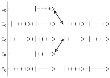
Figure 2: Lowest lying eigenstates of both the TLS Hamiltonian $H_{TLS}$ and the symmetry operator $\mathrm{\Pi}$ for $4$ two-level systems. The eigenenergies are $E_{0}=-3J$, $E_{a}=-J-2h_{1}-2h_{2}$, $E_{c}=-J-2h_{1}$, $E_{d}=-J+2h_{1}$ and $E_{b}=-J+2h_{1}+2h_{2}$. The states on the left (right) correspond to the eigenvalue $1$ ($-1$) of $\mathrm{\Pi}$. The arrowed lines connect the ’left’ and ’right’ states which are coupled by the monochromatic field.

4 TLS asymptotic state

For a large average boson number $\alpha^{2}$, there exists a time regime where its variation is negligible and the TLS chain reaches an asymptotic state $\rho_{\infty}$ CDG . To determine $\rho_{\infty}$, we first write the reduced density matrix of the system made up of the TLS and the monochromatic field, at positive times $t$, as

$$\rho_{TLS+F}(t)=\frac{i}{2\pi}\int_{\R+i\xi}dze^{-izt}\mathrm{Tr}_{\cal B}\left[\left(z-{\cal L}\right)^{-1}\Omega\right]$$ (8)

where $\mathrm{Tr}_{\cal B}$ denotes the partial trace over the heat bath, $\xi$ is a positive real number, and the Liouvillian ${\cal L}$ is defined by ${\cal L}\ldots=[H,\ldots]$. The matrix elements ${\hat{r}}_{k{\tilde{n}}l{\tilde{s}}}(z)={\langle k|\langle{\tilde{n}}|\mathrm{Tr}_{\cal B}[(z-{\cal L})^{-1}\Omega]|l\rangle|{\tilde{s}}\rangle}$ of the Laplace transform of $\rho_{TLS+F}$, can be written as

$${\hat{r}}_{k{\tilde{n}}l{\tilde{s}}}(z)=\sum_{k^{\prime},{\tilde{n}}^{\prime},l^{\prime},{\tilde{s}}^{\prime}}\Gamma_{k{\tilde{n}}l{\tilde{s}},k^{\prime}{\tilde{n}}^{\prime}l^{\prime}{\tilde{s}}^{\prime}}(z)r_{k^{\prime}l^{\prime}}\frac{\alpha^{{\tilde{n}}^{\prime}+{\tilde{s}}^{\prime}}}{\sqrt{{\tilde{n}}^{\prime}!{\tilde{s}}^{\prime}!}}e^{-\alpha^{2}}$$ (9)

where the functions $\Gamma_{k{\tilde{n}}l{\tilde{s}},k^{\prime}{\tilde{n}}^{\prime}l^{\prime}{\tilde{s}}^{\prime}}(z)$ depend only on the heat bath part of the initial state (3) EPJB2 . The right hand side of this equation can be read as the product of a square matrix ${\bf\Gamma}(z)$ with a column vector. A master equation for $\rho_{TLS+F}$ can then be derived with the help of the inverse matrix ${\bf\Sigma}={\bf\Gamma}^{-1}$, see Appendix A.

We are concerned with the limit of weak coupling of the TLS to their environment and with $\epsilon,\epsilon_{f}\ll e$. It is only in the limit of weak coupling to its surroundings, that the density matrix of an open system with Hamiltonian ${\cal H}$, relaxes to the canonical equilibrium state $\rho_{eq}\propto\exp(-{\cal H}/T)$ when its environment is in equilibrium with temperature $T$. To obtain $\rho_{\infty}$ in the regime of interest, the expansion of ${\bf\Sigma}$ to first order in $\epsilon_{f}$ and to second order in $e$ and $\epsilon$, is required. We find ${\bf\Sigma}={\bf\Sigma}^{0}+{\bf\Sigma}^{TLS\;{\cal B}}+\alpha^{-1}\epsilon_{f}{\bf\Sigma}^{TLS\;F}+\ldots$ where

$$\Sigma^{0}_{k{\tilde{n}}l{\tilde{s}},k^{\prime}{\tilde{n}}^{\prime}l^{\prime}{\tilde{s}}^{\prime}}= [z-\omega_{kl}+({\tilde{s}}-{\tilde{n}})\omega]\delta_{k^{\prime}k}\delta_{l^{\prime}l}\delta_{{\tilde{n}}^{\prime}{\tilde{n}}}\delta_{{\tilde{s}}^{\prime}{\tilde{s}}}$$ (10)

$$\Sigma^{TLS\;{\cal B}}_{k{\tilde{n}}l{\tilde{s}},k^{\prime}{\tilde{n}}^{\prime}l^{\prime}{\tilde{s}}^{\prime}}= -i\gamma_{kl,k^{\prime}l^{\prime}}\big{(}z+({\tilde{s}}-{\tilde{n}})\omega\big{)}\delta_{{\tilde{n}}^{\prime}{\tilde{n}}}\delta_{{\tilde{s}}^{\prime}{\tilde{s}}}$$ (11)

$$\Sigma^{TLS\;F}_{k{\tilde{n}}l{\tilde{s}},k^{\prime}{\tilde{n}}^{\prime}l^{\prime}{\tilde{s}}^{\prime}}= \delta_{k^{\prime}k}\sigma_{l^{\prime}l}\delta_{{\tilde{n}}^{\prime}{\tilde{n}}}\sqrt{{\tilde{s}}^{\prime}\delta_{{\tilde{s}}^{\prime}{\tilde{s}}+1}+{\tilde{s}}\delta_{{\tilde{s}}^{\prime}{\tilde{s}}-1}}\;$$

$$-\delta_{l^{\prime}l}\sigma_{kk^{\prime}}\delta_{{\tilde{s}}^{\prime}{\tilde{s}}}\sqrt{{\tilde{n}}\delta_{{\tilde{n}}^{\prime}{\tilde{n}}-1}+{\tilde{n}}^{\prime}\delta_{{\tilde{n}}^{\prime}{\tilde{n}}+1}}.$$

In these expressions, the notations $\omega_{kl}=E_{k}-E_{l}$ and $\sigma_{kl}=\langle k|\sigma_{N}^{x}|l\rangle$ have been used. The functions $\gamma_{kl,k^{\prime}l^{\prime}}$, which describe the influence of the heat bath, can be expressed in terms of bath time-dependent correlation functions, see Appendix B EPJB2 ; QDS ; CDG . For a large number $\alpha^{2}$ and a finite time $t$, the matrix element ${\langle k|\langle{\tilde{n}}|\rho_{TLS+F}|l\rangle|{\tilde{s}}\rangle}$ is non-negligible only if ${\tilde{n}}$ and ${\tilde{s}}$ are close to $\alpha^{2}$. Consequently, these integers can be replaced by $\alpha^{2}$ in (4). Since they appear in (10) and (11) only via the difference ${\tilde{s}}-{\tilde{n}}$, it is convenient to define

$${\hat{r}}^{(p)}_{kl}(z)=\sum_{{\tilde{n}}}{\hat{r}}_{k{\tilde{n}}l{\tilde{n}}+p}(z).$$ (13)

For $p=0$, this expression gives the matrix elements of the Laplace transform of the TLS chain state

$$\rho(t)=\mathrm{Tr}_{F}\rho_{TLS+F}(t)$$ (14)

where $\mathrm{Tr}_{F}$ denotes the partial trace over the monochromatic field.

As we are interested in the TLS asymptotic state, we write the column vector ${\bf r}(z)$ of elements ${\hat{r}}_{k{\tilde{n}}l{\tilde{s}}}(z)$ as ${\bf r}(z)=\sum_{x}{\bf r}_{x}/(z-x)+{\bf\tilde{r}}(z)$ where $x$ is real and ${\bf\tilde{r}}(z)$ has no singularity on the real axis. The potential pole at $z=x$, gives an undamped component of the TLS state, of frequency $x$, and hence contributes to $\rho_{\infty}$. Since the elements of the vector ${\bf\Sigma}(z){\bf r}(z)$ are equal to matrix elements of the TLS+field initial state, it is non-singular, and thus the vector ${\bf r}_{x}$ must fulfill ${\bf\Sigma}(i0^{+}+x){\bf r}_{x}=0$. Let us focus on the term $x=0$, which always exists, and denote by ${\bf u}$ the zeroth order of ${\bf r}_{0}$ in an expansion in terms of $e$, $\epsilon$ and $\epsilon_{f}$. Similarly to (13), we define $u^{(p)}_{kl}$ from the elements of ${\bf u}$. From ${\bf\Sigma}^{0}(i0^{+}){\bf u}=0$, it ensues that $u^{(p)}_{kl}$ is non-vanishing only if $\omega_{kl}=p\omega$. Then, from the next order terms of ${\bf\Sigma}(i0^{+}){\bf r}_{0}=0$, we obtain

$$\epsilon_{f}\sum_{j}\Big{[}\sigma_{jl}\big{(}{u}^{(p+1)}_{kj}+{u}^{(p-1)}_{kj}\big{)}-\sigma_{kj}\big{(}{u}^{(p+1)}_{jl}+{u}^{(p-1)}_{jl}\big{)}\Big{]}\\ -i\sum_{k^{\prime},l^{\prime}}\gamma_{kl,k^{\prime}l^{\prime}}(i0^{+}+p\omega){u}^{(p)}_{k^{\prime}l^{\prime}}=0,$$ (15)

where $k$, $l$ and $p$ are such that $\omega_{kl}=p\omega$ and ${u}^{(p^{\prime})}_{k^{\prime}l^{\prime}}=0$ if $\omega_{k^{\prime}l^{\prime}}\neq p^{\prime}\omega$. If $\omega$ is chosen arbitrarily and is not equal to any $\omega_{kl}/p$ then the only non-vanishing ${u}^{(p)}_{kl}$ obey $p=0$ and $E_{k}=E_{l}$, and are solutions of equation (15) with no monochromatic field term. In this case, the field influence manifests itself only through higher order corrections. In the opposite case, for a resonant field frequency, the dominant contribution to the asymptotic behavior is affected by the coupling to the monochromatic field. For the more general TLS-field coupling $\alpha^{-1}\epsilon_{f}\sum_{n,\nu}\sigma^{\nu}_{n}(\lambda_{n\nu}a^{\dagger}+\lambda_{n\nu}^{*}a)$, in the first line of equation (15), $\sigma_{kl}$ is replaced by $\sum_{n,\nu}\lambda_{n\nu}\langle k|\sigma_{n}^{\nu}|l\rangle$ in the first and third terms, and by $\sum_{n,\nu}\lambda_{n\nu}^{*}\langle k|\sigma_{n}^{\nu}|l\rangle$ in the second and fourth ones.

Since ${u}^{(0)}_{kl}=0$ if $\omega_{kl}\neq 0$, the matrix elements $\langle k|\rho|l\rangle$ of the TLS state (14) such that $E_{k}\neq E_{l}$, have no steady component. Moreover, it is clear from the expression (10), that, for $\omega_{kl}=0$, the only possible undamped component of $\langle k|\rho|l\rangle$ is of zero frequency, and hence

$$\langle k|\rho_{\infty}|l\rangle={u}^{(0)}_{kl}$$ (16)

for $E_{k}=E_{l}$. Actually, the other non-vanishing ${u}^{(p)}_{kl}$ give also contributions to $\rho_{\infty}$. This can be seen as follows. Let us define the vector ${\bf r}_{P\omega}$ of elements $({\bf r}_{0})_{k{\tilde{n}}l{\tilde{s}}+P}$. It satisfies ${\bf\Sigma}(i0^{+}+P\omega){\bf r}_{P\omega}=0$ with the approximate ${\bf\Sigma}$ discussed above, and thus, corresponds to a pole of ${\bf r}(z)$ on the real axis at $z=P\omega$. Moreover, $\sum_{\tilde{n}}({\bf r}_{P\omega})_{k{\tilde{n}}l{\tilde{n}}}=\sum_{\tilde{n}}({\bf r}_{0})_{k{\tilde{n}}l{\tilde{n}}+P}$ is equal to $u_{kl}^{(P)}$ to zeroth order, and hence (16) generalizes to $\langle k|\rho_{\infty}|l\rangle={u}^{(p)}_{kl}\exp(-ip\omega t)$ for $E_{k}=E_{l}+p\omega$. In Appendix A, we derive from (10)-(4), a Markovian master equation for $\rho(t)$ which reduces to Redfield equation when $\epsilon_{f}=0$, and show that a time-periodic $\rho=\sum_{p}\exp(-ip\omega t)\varrho^{(p)}$ satisfies this equation only if $\varrho^{(p)}_{kl}=u_{kl}^{(p)}$ to lowest order in $e$, $\epsilon$ and $\epsilon_{f}$. In this Appendix, we also show that, in the case of a single TLS coupled to a zero-temperature bath, (15) gives the same asymptotic state as that obtained from the optical Bloch equations in the rotating wave approximation CDG .

5 Schrödinger cat regime

In this section, we consider the case of a field frequency

$$\omega=2h_{N}=E_{c}-E_{a}=E_{b}-E_{d},$$ (17)

see Fig.2, and of a low heat bath temperature,

$$T\ll h_{n}<J.$$ (18)

We will see that, in this limit, the asymptotic state $\rho_{\infty}$ is a steady state of the form

$$\rho_{\infty}=p|\mathrm{Scs}^{-}\rangle\langle\mathrm{Scs}^{-}|+(1-p)|\mathrm{Scs}^{+}\rangle\langle\mathrm{Scs}^{+}|$$ (19)

where the Schrödinger cat states $|\mathrm{Scs}^{\mp}\rangle$ are given by (6). For vanishing coupling to the monochromatic field, $\epsilon_{f}=0$, $p=1/2$ and $\rho_{\infty}=({|\!\Uparrow\rangle}{\langle\Uparrow\!|}+{|\!\Downarrow\rangle}{\langle\Downarrow\!|})/2$ is simply the zero temperature thermal state corresponding to the TLS Hamiltonian $H_{TLS}$. For $\epsilon_{f}\gg\epsilon$, $p=1$ and the TLS asymptotic state is a pure Schrödinger cat state. At the end of this section, it is shown that, provided $p\neq 1/2$, the mixed state (19) is not as highly entangled but remains nevertheless multipartite entangled. To obtain (19), we first define $\rho_{s}=\sum_{k,l}{u}^{(0)}_{kl}|k\rangle\langle l|$, which is the steady component of $\rho_{\infty}$. From (16) and Cauchy-Schwarz inequality, it follows that any matrix element of $\rho_{\infty}$ satisfies $|\langle k|\rho_{\infty}|l\rangle|^{2}\leq\langle k|\rho_{s}|k\rangle\langle l|\rho_{s}|l\rangle$, and that $\langle k|\rho_{\infty}|l\rangle=\langle k|\rho_{s}|l\rangle$ if $E_{k}=E_{l}$. In the following, we focus on $\rho_{s}$ and show that its only nonvanishing elements in the limit (18), are $\langle\mathrm{Scs}^{\mp}|\rho_{s}|\mathrm{Scs}^{\mp}\rangle$, which leads to the result (19).

5.1 No thermal equilibrium Schrödinger cat

Before embarking on the determination of $\rho_{\infty}$, let us first show that the thermal equilibrium state $\rho_{eq}$ of any TLS system cannot be of the form (19) with $p\neq 1/2$, in the absence of long range interactions. At temperature $T$, $\rho_{eq}\propto\sum_{k}|k\rangle\langle k|\exp(-E_{k}/T)$ where $|k\rangle$ and $E_{k}$ are the eigenstates and eigenenergies of the TLS Hamiltonian ${\cal H}$. If the temperature is too high, $\rho_{eq}$ is a mixture of a large number of states. At zero temperature, $\rho_{eq}$ is the equal-weight mixture of the ground states of ${\cal H}$. Thus, in this case, $\rho_{eq}$ can be of the form (19) but with $p=1/2$ only. The thermal state is given by $\rho_{eq}=p{|0\rangle\langle 0|}+(1-p){|1\rangle\langle 1|}$ with $p\neq 1/2$, only if $|0\rangle$ and $|1\rangle$ are the ground state and first excited state of ${\cal H}$, and are non-degenerate, and only in the limit $E_{2}\gg T$. We thus assume that ${\cal H}$ has a nondegenerate ground state $|0\rangle$. When no long range interaction is present, ${\cal H}$ can be decomposed as ${\cal H}={\cal H}_{1}+{\cal H}^{\prime}$ where no observable of TLS $1$ appears in ${\cal H}^{\prime}$ and there exists a TLS $n\neq 1$ which is not affected by ${\cal H}_{1}$. It can be proved that $|0\rangle$ cannot be ${|\mathrm{Scs}^{\mp}\rangle}$ by evaluating the average value $A={\langle\mathrm{Scs}^{\mp}|{\cal H}|\mathrm{Scs}^{\mp}\rangle}$ as follows. Since ${\langle\Downarrow\!|{\cal H}^{\prime}|\!\Uparrow\rangle}\propto{{{}_{1}\langle}-|+\rangle_{1}}=0$, and similarly for ${\cal H}_{1}$, $A=[{\langle\Downarrow\!|{\cal H}|\!\Downarrow\rangle}+{\langle\Uparrow\!|{\cal H}|\!\Uparrow\rangle}]/2$. Consequently, $A>{\langle 0|{\cal H}|0\rangle}$, as this last value is the minimum possible one for the average energy, and $|0\rangle$ cannot be both ${|\!\Uparrow\rangle}$ and ${|\!\Downarrow\rangle}$. Thus, $|0\rangle$ is not $|\mathrm{Scs}^{\mp}\rangle$. This result generalizes to all Schmidt decomposable states, see Appendix C.

5.2 Uniform coupling to the heat bath

As we are interested in the limits $\epsilon,\epsilon_{f}\ll e$, we first consider the case $\epsilon=\epsilon_{f}=0$. For these particular values, the total Hamiltonian (1) commutes with the symmetry operator $\mathrm{\Pi}$ defined by (5), and there thus exist several TLS asymptotic states. This can be seen as follows. Consider that the TLS initial state $\sum_{k,l}r_{kl}|k\rangle\langle l|$ is a statistical mixture of eigenstates of $\mathrm{\Pi}$ with eigenvalue $1$. Since $[H,\mathrm{\Pi}]=0$, the TLS reduced state at any time is also such a mixture. The conclusion is obviously similar for the eigenvalue $-1$ and hence the asymptotic state cannot be the same for these two kinds of initial states. Note that this argument is valid for any coupling strength $e$. We remark that, though $H_{TLS}$ and $S_{x}=\sum_{n}\sigma^{x}_{n}$ both commute with the symmetry operator $\mathrm{\Pi}$, they do not have, for general values of $J$ and $h_{n}$, any common eigenvector, and hence that there is no decoherence-free subspace in the TLS Hilbert space ZR , see Appendix D.

For $\epsilon_{f}=0$, equations (15) separate into the independent equation sets $\sum_{k^{\prime},l^{\prime}}\gamma_{kl,k^{\prime}l^{\prime}}(i0^{+}+p\omega){u}^{(p)}_{k^{\prime}l^{\prime}}=0$, where $k$ and $l$ are such that $\omega_{kl}=p\omega$, and ${u}^{(p)}_{k^{\prime}l^{\prime}}=0$ if $\omega_{k^{\prime}l^{\prime}}\neq p\omega$. The equation set $p=0$ gives the steady component $\rho_{s}=\sum_{k,l}{u}^{(0)}_{kl}|k\rangle\langle l|$ of $\rho_{\infty}$. Up to now, the basis set $\{|k\rangle\}$ has not been fully specified. The states $|k\rangle$ are eigenstates of $H_{TLS}$, but, for a degenerate energy level $E_{k}$, infinitely many choices are possible. To obtain the expression of $\rho_{s}$, we consider the diagonalized form of this density matrix in the appropriate unknown basis set $\{|k\rangle\}$. The equations

$$\sum_{k^{\prime}}\gamma_{kl,k^{\prime}k^{\prime}}(i0^{+}){u}^{(0)}_{k^{\prime}k^{\prime}}=0$$ (20)

where $k$ and $l$ are such that $E_{k}=E_{l}$, then determine both $\{|k\rangle\}$ and the populations $u^{(0)}_{kk}$. Let us introduce the coefficients $\Upsilon_{kl}=\gamma_{kk,ll}(i0^{+})\exp(-E_{l}/T)$. They obey $\Upsilon_{lk}=\Upsilon_{kl}$ and $\sum_{k}\Upsilon_{kl}=0$, see Appendix B, and hence, for any set $\{\varphi_{k}\}$,

$$\sum_{k,l}\Upsilon_{kl}\varphi_{k}\varphi_{l}=-\frac{1}{2}\sum_{k,l}\Upsilon_{kl}(\varphi_{k}-\varphi_{l})^{2}.$$ (21)

By definition of $\Upsilon_{kl}$, this sum vanishes for $\varphi_{k}=u_{kk}^{(0)}\times\exp(E_{k}/T)$. Since $\Upsilon_{lk}=\Upsilon_{kl}$ and $\Upsilon_{kl}\geq 0$ for $k\neq l$, the vanishing of (21) is equivalent to $\sum_{l}\Upsilon_{kl}\varphi_{l}=0$ . As shown in Appendix B, for $k\neq l$, $\Upsilon_{kl}$ is proportionnal to $S_{kl}=\langle k|S_{x}|l\rangle^{2}$ when $\epsilon=0$. Since the right hand side of (21) is equal to zero only if $\varphi_{k}=\varphi_{l}$ when $\Upsilon_{kl}\neq 0$, $u^{(0)}_{kk}/u^{(0)}_{ll}=\exp(-\omega_{kl}/T)$ when $S_{kl}\neq 0$. This relation ensures that the equations (20) with $k\neq l$, are satisfied, see Appendix B.

Thus, $\rho_{s}$ is determined by the equations (20) with $k=l$, or, equivalently, by the vanishing of the sum (21). It can always be written as

$$\rho_{s}=\sum_{q}\frac{p_{q}}{z_{q}}\sum_{k\in{\cal E}_{q}}e^{-E_{k}/T}|k\rangle\langle k|,$$ (22)

where $z_{q}=\sum_{k\in{\cal E}_{q}}\exp(-E_{k}/T)$ and $\sum_{q}p_{q}=1$. This expression satisfies (20) if the states $|k\rangle$ and the sets ${\cal E}_{q}$ are such that $S_{kl}=0$ for any $k\in{\cal E}_{q}$ and $l\in{\cal E}_{q^{\prime}}$ where $q^{\prime}\neq q$. Obviously, as soon as there exist more than one set ${\cal E}_{q}$, the decomposition (22) is not unique, as a new family of sets ${\cal E}_{q}$ can be simply defined by unioning sets. Thus, we assume that a set ${\cal E}_{q}$ cannot be divided into subsets ${\cal E}_{q^{\prime}}$ and ${\cal E}_{q^{\prime\prime}}$ such that $S_{kl}=0$ for any $k\in{\cal E}_{q}^{\prime}$ and $l\in{\cal E}_{q^{\prime\prime}}$. In this case, every state $|k\rangle$ in (22), is eigenstate of $\mathrm{\Pi}$ and the value of the corresponding eigenvalue depends only on the set ${\cal E}_{q}$ to which $k$ belongs. This can be shown as follows. Consider the subspace ${\cal S}_{q}$ of the TLS Hilbert space, spanned by $\{|k\rangle\}$ where $k\in{\cal E}_{q}$. It can always be decomposed as ${\cal S}_{q}={\cal S}_{q+}\oplus{\cal S}_{q-}$ where ${\cal S}_{q\pm}$ is spanned by the states $(1\pm\mathrm{\Pi}){|k\rangle}$, which are eigenstates of both $H_{TLS}$ and $\mathrm{\Pi}$. Since $[S_{x},\mathrm{\Pi}]=0$, $\langle\psi|S_{x}|\psi^{\prime}\rangle=0$ for any $|\psi\rangle\in{\cal S}_{q+}$ and $|\psi^{\prime}\rangle\in{\cal S}_{q-}$. As ${\cal E}_{q}$ cannot be subdivided, as assumed above, ${\cal S}_{q}={\cal S}_{q+}$ or ${\cal S}_{q}={\cal S}_{q-}$. In other words, all the states $|k\rangle$ given by ${\cal E}_{q}$, are such that $\mathrm{\Pi}|k\rangle=\pm|k\rangle$. For $N=2$, the number of levels $E_{k}$ is small enough to allow the complete determination of the minimal sets ${\cal E}_{q}$. For general values of $J$ and $h_{n}$, there are only two sets, corresponding to the two eigenvalues of $\mathrm{\Pi}$. For $h_{2}=0$, there are three sets, one giving only the state $({|+-++\rangle}-{|--+-\rangle}-{|++-+\rangle}+{|-+--\rangle})/2$. We remark that, since this state is eigenstate of both $H_{TLS}$ and $S_{x}$, it is decoherence-free, see Appendix D. The situation is similar for $h_{1}=0$ and $h_{2}=h_{1}$.

For our purpose, we only need to know a few states $|k\rangle$ and the corresponding two sets ${\cal E}_{q}$. The two ground states $|\mathrm{Scs}^{-}\rangle$ and $|\mathrm{Scs}^{+}\rangle$ are eigenstates of $\mathrm{\Pi}$ with eigenvalues $-1$ and $1$, respectively. Thus, they are given by two different sets, ${\cal E}_{-}$ and ${\cal E}_{+}$. Consider the doubly degenerate energy levels $E_{e}$ and $E_{f}$ corresponding, respectively, to the states $|e^{\pm}\rangle={\cal I}_{\pm}|+\rangle_{1}|-\rangle_{2}\ldots$ and $|f^{\pm}\rangle={\cal I}_{\pm}|-\rangle_{1}|+\rangle_{2}\ldots$, where ${\cal I}_{\pm}=2^{-1/2}(1\pm\mathrm{\Pi})$ . Since $S_{\mathrm{Scs}^{\pm}e^{\pm}}=S_{\mathrm{Scs}^{\pm}f^{\pm}}=1$, $e^{\pm}$ and $f^{\pm}$ belong to ${\cal E}_{\pm}$. By evaluating the matrix elements of $S_{x}$ between the one-interface states discussed at the end of section 3, and noting that the degeneracy of a one-interface level is $1$ or $2$, it can be shown that ${\cal E}_{+}$ gives all the states ${\cal I}_{+}|\mbox{\large$\eta$}\rangle$ where $|\mbox{\large$\eta$}\rangle$ is a one-interface configuration state which is not eigenstate of $\mathrm{\Pi}$, $|a\rangle$, $|b\rangle$, and $|\mathrm{Scs}^{+}\rangle$. Similarly, ${\cal E}_{-}$ gives all the states ${\cal I}_{-}|\mbox{\large$\eta$}\rangle$ and $|\mathrm{Scs}^{-}\rangle$.

5.3 General coupling to the heat bath

The non-uniqueness of $\rho_{s}$ for $\epsilon=\epsilon_{f}=0$ stems from the particular form of the coupling to the environment in this case. If the uniformity of this coupling is broken, even slightly, this indeterminacy disappears, as we show here. For $\epsilon\neq 0$ and $\epsilon_{f}=0$, the potential sets ${\cal E}_{q}$, appearing in the decomposition (22), are determined by $e\langle k|S_{x}|l\rangle\langle A|\pi|B\rangle+\epsilon\sum_{n,\nu}\langle k|\sigma^{\nu}_{n}|l\rangle\langle A|\pi^{\nu}_{n}|B\rangle=0$ where $|A\rangle$ and $|B\rangle$ are any eigenstates of the bath Hamiltonian $H_{\cal B}$, since $\Upsilon_{kl}$ vanishes only if this condition is satisfied, see Appendix B. In general, it is equivalent to $\langle k|\sigma^{\nu}_{n}|l\rangle=0$ for any $n$ and $\nu$. In other words, $k$ and $l$ belong to the same set ${\cal E}_{q}$ if $\langle k|\sigma^{\nu}_{n}|l\rangle\neq 0$ for some $n$ and $\nu$. As a consequence, $k$ and $l$ belong to the same set ${\cal E}_{q}$ if there exist ${\tilde{\jmath}}_{1}$, …, ${\tilde{\jmath}}_{s}$, $n_{1}$, …, $n_{s}$, $n$, $\nu_{1}$, …, $\nu_{s}$ and $\nu$ such that $\langle k|\otimes_{r}(\sigma_{n_{r}}^{\nu_{r}}|{\tilde{\jmath}}_{r}\rangle\langle{\tilde{\jmath}}_{r}|)\sigma_{n}^{\nu}|l\rangle\neq 0$, which means that there is a bath-induced transition path between the states $|k\rangle$ and $|l\rangle$. Since

$$\sum_{j_{1},\ldots,j_{s}}\Big{|}\langle k|\sigma_{n_{1}}^{\nu_{1}}|j_{1}\rangle\prod_{r=2}^{s}\langle j_{r-1}|\sigma_{n_{r}}^{\nu_{r}}|j_{r}\rangle\langle j_{s}|\sigma_{n}^{\nu}|l\rangle\Big{|}\\ \geq\Big{|}\langle k|\otimes_{r=1}^{s}\sigma_{n_{r}}^{\nu_{r}}\sigma_{n}^{\nu}|l\rangle\Big{|},$$ (23)

$k$ and $l$ belong to the same set ${\cal E}_{q}$ if there exist $n_{1}$, …, $n_{s}$, $n$, $\nu_{1}$, …, $\nu_{s}$ and $\nu$ such that $\langle k|\otimes_{r}\sigma_{n_{r}}^{\nu_{r}}\sigma_{n}^{\nu}|l\rangle\neq 0$. Consider any state $|k\rangle$ appearing in (22). It can be expanded on the basis of configuration states ${|\mbox{\large$\eta$}_{r}\rangle}=\mathop{\hbox{\c\char 10\relax}}_{n}{|\eta_{rn}\rangle_{n}}$ as ${|k\rangle}=\sum_{r}\lambda_{r}{|\mbox{\large$\eta$}_{r}\rangle}$, which can be rewritten as ${|k\rangle}=\sum_{r}\lambda_{r}\otimes_{n}{(\sigma^{x}_{n})^{\tau_{rn}}}{|a\rangle}$ where ${|a\rangle}={|+\rangle_{1}\ldots|-\rangle_{N+1}\ldots}$, and $\tau_{rn}$ is equal to $1/2+\eta_{rn}/2$ for $n>N$ and to $1/2-\eta_{rn}/2$ otherwise. As the eigenenergy $E_{a}$ is nondegenerate, $|a\rangle$ is necessarily present in (22). Since at least one $\lambda_{r}$ is nonzero and $\langle a|\otimes_{n}(\sigma^{x}_{n})^{\tau_{rn}}|k\rangle=\lambda_{r}$ for any $r$, $a$ and $k$ belong to the same set ${\cal E}_{q}$. Thus, there is a unique set ${\cal E}_{q}$ and $\rho_{s}=\rho_{eq}\propto\sum_{k}\exp(-E_{k}/T){|k\rangle}{\langle k|}$ is the thermal state of the TLS system. Consequently, in the low temperature limit (18), $\rho_{\infty}=\rho_{s}=({|\!\Uparrow\rangle}{\langle\Uparrow\!|}\pm{|\!\Downarrow\rangle}{\langle\Downarrow\!|})/2$, which can be written as (19) with $p=1/2$. We remark that the above proof applies even if $\pi_{n}^{y}=\pi_{n}^{z}=0$, and that the only required assumption on the parameters of $H_{TLS}$ is that they are generic enough that $E_{a}$ is non-degenerate.

5.4 Low temperature limit

In this section, we show that, for any $\epsilon_{f}$ and any ${\epsilon\neq 0}$, $\langle k|\rho_{s}|l\rangle$ vanishes in the low temperature limit (18), if $E_{k}=E_{l}$ is larger than $E_{0}+3J$. This result, together with those of section 5.2, lead, for $\epsilon,\epsilon_{f}\ll e$, to the form (19) for $\rho_{\infty}$. Let us first write $\rho_{s}=\sum_{k}u_{kk}^{(0)}|k\rangle\langle k|$ in diagonal form, and observe that, if $E_{l}<E_{k}$, $\gamma_{kk,ll}(i0^{+})$ vanishes at low temperatures, see expression (B), and that, for any $l$ such that $E_{l}>E_{a}$, there exists $k$ such that $E_{k}<E_{l}$ and $\gamma_{kk,ll}(i0^{+})\neq 0$. In other words, the upward transition rates vanish at zero temperature, and there is a downward transition from any excited state but the first one ${|a\rangle}={|+\rangle_{1}\ldots|-\rangle_{N+1}\ldots}$. This last property can be seen as follows. Except the ground states ${|\!\Uparrow\rangle}$ and ${|\!\Downarrow\rangle}$, and the one-interface states ${|\pm\rangle_{1}|\mp\rangle_{2}\ldots}$ and ${\ldots|\pm\rangle_{2N-1}|\mp\rangle_{2N}}$, any configuration state ${|\mbox{\large$\eta$}\rangle}$ presents a sequence ${|\pm\rangle_{n}}{|\mp\rangle_{n+1}}$ where $n\notin\{1,2N-1\}$. Thus, if ${|\mbox{\large$\eta$}\rangle}$ is neither one of the states mentioned above, nor ${|\pm\rangle_{1}\ldots|\mp\rangle_{N+1}\ldots}$, it contains a sequence ${|\mp\rangle_{n-1}|\pm\rangle_{n}|\mp\rangle_{n+1}}$ where $n\notin\{1,2N-1\}$, or a sequence ${|\pm\rangle_{n-1}|\pm\rangle_{n}|\mp\rangle_{n+1}|\mp\rangle_{n+2}}$ where $n\notin\{1,N,2N-1\}$. In the first case, the energy of $\sigma_{n}^{x}{|\mbox{\large$\eta$}\rangle}$ is lower than that of ${|\mbox{\large$\eta$}\rangle}$ of $-2J\pm 2{\tilde{h}}_{n}$ where ${\tilde{h}}_{n}=-h_{2N+1-n}$ for $n>N$ and $h_{n}$ otherwise. In the second case, the difference between the energies of ${|\mbox{\large$\eta$}\rangle}$ and of $\sigma_{n}^{x}{|\mbox{\large$\eta$}\rangle}$ is $\pm 2{\tilde{h}}_{n}$, and that between the energies of ${|\mbox{\large$\eta$}\rangle}$ and of $\sigma_{n+1}^{x}{|\mbox{\large$\eta$}\rangle}$ is $\mp 2{\tilde{h}}_{n+1}$. Consequently, since $h_{n}>0$, there always exists a configuration state $\sigma_{n}^{x}{|\mbox{\large$\eta$}\rangle}$ with one TLS flipped, of energy lower than that of ${|\mbox{\large$\eta$}\rangle}$. This result can be extended to the states ${|\pm\rangle_{1}|\mp\rangle_{2}\ldots}$ and ${\ldots|\pm\rangle_{2N-1}|\mp\rangle_{2N}}$, since flipping, respectively, the first and the last TLS, leads to one of the two ground states ${|\!\Uparrow\rangle}$ or ${|\!\Downarrow\rangle}$, and to ${|b\rangle}={|-\rangle_{1}\ldots|+\rangle_{N+1}\ldots}$, since the energy of $\sigma_{N}^{x}{|b\rangle}$ and $\sigma_{N+1}^{x}{|b\rangle}$ is $E_{d}=E_{b}-2h_{N}$, see Fig.2. Thus, $|a\rangle$ is the only exception. Consider now any $l\neq a$ and expand the corresponding state on the appropriate configuration state basis as $|l\rangle=\sum_{r=1}^{s}\lambda_{r}{|\mbox{\large$\eta$}_{r}\rangle}$. As seen above, there exists $n$ such that the energy $E_{k}$ of $\sigma_{n}^{x}{|\mbox{\large$\eta$}_{1}\rangle}$ is lower than $E_{l}$. There are possibly $s^{\prime}$ states $\sigma_{n}^{x}{|\mbox{\large$\eta$}_{r}\rangle}$ of energy $E_{k}$. The state ${|\psi\rangle}=\sum_{r=1}^{s^{\prime}}\lambda_{r}\sigma_{n}^{x}{|\mbox{\large$\eta$}_{r}\rangle}$ belongs to the TLS Hilbert subspace spanned by the states $|k\rangle$ of energy $E_{k}$. Consequently, there is at least one $|k\rangle$ such that ${\langle k|\sigma_{n}^{x}|l\rangle}={\langle k|\psi\rangle}\neq 0$, and hence, such that $\gamma_{kk,ll}(i0^{+})\neq 0$.

We now consider equation (15) with $p=0$ and $T=0$. Any eigenenergy $E_{k}$ is of the form $E_{k}=E_{0}+2mJ+\sum_{n}h_{n}\tau_{n}$ where $\tau_{n}\in\{-2,0,2\}$ and $m$ is the number of interfaces of the corresponding configuration states. Consequently, for general values of $J$ and $h_{n}$, if $\omega_{kl}=\pm\omega=\pm 2h_{N}$ then $k$ and $l$ correspond to the same number $m$ of interfaces. In particular, the monochromatic field does not couple one-interface states to multi-interface states. Therefore, at $T=0$,

$$\epsilon_{f}\sum_{l\in{\cal A}_{H}}\Big{[}\sigma_{lk}\big{(}{u}^{(1)}_{kl}+{u}^{(-1)}_{kl}\big{)}-\sigma_{kl}\big{(}{u}^{(1)}_{lk}+{u}^{(-1)}_{lk}\big{)}\Big{]}\\ -i\sum_{l\in{\cal A}_{H}}(\gamma_{kl}{u}^{(0)}_{ll}-\gamma_{lk}{u}^{(0)}_{kk})+i\sum_{l\in{\cal A}_{L}}\gamma_{lk}{u}^{(0)}_{kk}=0,$$ (24)

where $\gamma_{kl}$ is the zero temperature limit of $\gamma_{kk,ll}(i0^{+})$, ${\cal A}_{H}=\{k:E_{k}>E_{0}+3J\}$, ${\cal A}_{L}=\{k:E_{k}<E_{0}+3J\}$, and $k\in{\cal A}_{H}$. The solution to this equation set can be interpreted as the asymptotic state of a system evolving under the influence of a zero temperature heat bath, a monochromatic field, and an additional decay mechanism characterized by the rates $\sum_{l\in{\cal A}_{L}}\gamma_{lk}$. Equation (24) leads to $\sum_{k\in{\cal A}_{H},l\in{\cal A}_{L}}\gamma_{lk}{u}^{(0)}_{kk}=0$. Since all the coefficients $\gamma_{lk}$ in this sum are positive, ${u}^{(0)}_{kk}=0$ if one $\gamma_{lk}$ is different from zero. The results obtained above show that this is the case for $k\in{\cal A}_{H}$ corresponding to the lowest $E_{k}$ given by this set. Thus, ${u}^{(0)}_{kk}={u}^{(\pm 1)}_{kl}={u}^{(\pm 1)}_{lk}=0$ for these $k$, and, in the equations (24) determining the other ${u}^{(0)}_{kk}$ where $k\in{\cal A}_{H}$, the sets ${\cal A}_{H}$ and ${\cal A}_{L}$ can be replaced by the sets ${\cal A}^{\prime}_{H}$ and ${\cal A}^{\prime}_{L}$ obtained by, respectively, removing these $k$ from ${\cal A}_{H}$ and adding them to ${\cal A}_{L}$. This new equation set leads to ${u}^{(0)}_{kk}={u}^{(\pm 1)}_{kl}={u}^{(\pm 1)}_{lk}=0$ for $k\in{\cal A}^{\prime}_{H}$ corresponding to the lowest $E_{k}$ given by this set. By repeating this procedure, it can be shown that ${u}^{(0)}_{kk}=0$ for all $k\in{\cal A}_{H}$, i.e., such that $E_{k}>E_{0}+3J$.

For $\epsilon,\epsilon_{f}\ll e$, we know that $\rho_{s}$ is given by (22). The results of this section show that the probabilities $p_{q}$ where $q\neq\pm$, vanish at low temperatures, since the corresponding sets ${\cal E}_{q}$ give states with more than one interface. Thus, the low temperature TLS asymptotic state is of the form (19). By slightly modifying the above derivation, it can be shown that $p_{q}\ll\exp(-3J/T)$ where $q\neq\pm$. At low temperatures, $\gamma_{kk,ll}(i0^{+})\simeq\gamma_{lk}\exp(-\omega_{kl}/T)$ if $E_{l}<E_{k}$, see expression (B). Hence, the terms neglected in equation (24), are approximatively given by $-i\sum_{l\in{\cal A}_{L}}\gamma_{lk}\times\exp(-\omega_{kl}/T){u}^{(0)}_{ll}$. Since ${u}^{(0)}_{ll}\simeq p_{\pm}\exp[-(E_{l}-E_{0})/T]$ for $l\in{\cal E}_{\pm}$, and ${\cal A}_{L}\subset{\cal E}_{+}\cup{\cal E}_{-}$, the above sum is far smaller than $\exp(-3J/T)$, and hence $\exp(3J/T){u}^{(0)}_{kk}$ where $k\in{\cal A}_{H}$, vanishes in the zero temperature limit. This result will be useful in the following.

5.5 Steady Schrödinger cat state

We assume here that $\epsilon\ll\epsilon_{f}\ll e$. To obtain $\rho_{s}$ in this case, it is convenient to first rewrite equations (15) in matrix form as ${\bf G}_{0}^{(p)}{\bf u}^{(p)}+\epsilon_{f}{\bf G}_{1}^{(p)}{\bf u}^{(p+1)}+\epsilon_{f}{\bf G}_{-1}^{(p)}{\bf u}^{(p-1)}{=0}$ where ${\bf u}^{(p)}$ is the column vector whose elements are the non-vanishing $u^{(p)}_{kl}$, i.e., such that $\omega_{kl}=p\omega$. In the following, we use the inverse matrices $({\bf G}_{0}^{(p)})^{-1}$ where $p\neq 0$. Their existence can be shown as follows. If $0$ were an eigenvalue of ${\bf G}_{0}^{(p)}$, possible asymptotic states for $\epsilon_{f}=0$, would be $\rho_{\infty}=\rho_{eq}+x\rho_{osc}$ where $\rho_{osc}$ is a matrix with only nondiagonal elements, oscillating at frequency $p\omega$, constructed from an eigenvector of ${\bf G}_{0}^{(p)}$ with eigenvalue $0$, and $x$ is any real number. But, since $\rho_{\infty}$ is a density matrix, its off-diagonal elements obey $x^{2}|\langle k|\rho_{osc}|l\rangle|^{2}<1$, which is not possible for any $x$ if $\rho_{osc}\neq 0$. Thus, $0$ is not an eigenvalue of ${\bf G}_{0}^{(p)}$, which is hence invertible. Physically, this means that the possible oscillating components of $\rho_{\infty}$ with frequencies $p\omega$, are induced by the monochromatic field and disappear when the coupling to it vanishes. As a consequence, the contribution to $\rho_{\infty}$ which oscillates at frequency $\omega$ has an amplitude of the order of $\epsilon_{f}$, and, more generally, ${\bf u}^{(p)}$ is of the order of $\epsilon_{f}^{|p|}$. Thus, ${\bf u}^{(0)}$ satisfies

$$\left[{\bf G}_{0}^{(0)}-\epsilon_{f}^{2}{\bf G}_{1}^{(0)}\left({\bf G}_{0}^{(1)}\right)^{-1}{\bf G}_{-1}^{(1)}\right.\\ \left.-\epsilon_{f}^{2}{\bf G}_{-1}^{(0)}\left({\bf G}_{0}^{(-1)}\right)^{-1}{\bf G}_{1}^{(-1)}\right]{\bf u}^{(0)}=0,$$ (25)

where terms of order $\epsilon_{f}^{3}$ and higher have been neglected.

We denote by ${\bf\tilde{G}}_{0}^{(p)}$ the matrix ${\bf G}_{0}^{(p)}$ with $\epsilon$ set to zero. As seen in section 5.2, ${\bf\tilde{G}}_{0}^{(0)}$ has several eigenvectors ${\bf\Psi}_{q}$ with eigenvalue $0$, whose elements are $z_{q}^{-1}\exp(-E_{k}/T)\delta_{kl}$ if $k\in{\cal E}_{q}$ and $0$ otherwise, with the basis set $\{|k\rangle\}$ considered in section 5.2. There also exist column vectors ${\bf\Phi}_{q}$ which obey ${\bf\Phi}_{q}^{T}{\bf\tilde{G}}^{(0)}_{0}=0$ and ${\bf\Phi}_{q}^{T}{\bf\Psi}_{q^{\prime}}=\delta_{qq^{\prime}}$, and whose elements are $\delta_{kl}$ if $k\in{\cal E}_{q}$ and $0$ otherwise, see Appendix B. To zeroth order in $\epsilon_{f}$ and $\epsilon$, ${\bf u}^{(0)}=\sum_{q}p_{q}{\bf\Psi}_{q}$. Replacing ${\bf u}^{(0)}$ by this expression in (25) and neglecting terms proportional to powers of $\epsilon$, leads to $\sum_{q^{\prime}}r_{qq^{\prime}}p_{q^{\prime}}=0$ with

$$r_{qq^{\prime}}={\bf\Phi}_{q}^{T}\left[{\bf G}_{1}^{(0)}{\bf F}^{(1)}{\bf G}_{-1}^{(1)}+{\bf G}_{-1}^{(0)}{\bf F}^{(-1)}{\bf G}_{1}^{(-1)}\right]{\bf\Psi}_{q^{\prime}}$$ (26)

where ${\bf F}^{(\pm 1)}=({\bf\tilde{G}}_{0}^{(\pm 1)})^{-1}$. Since the monochromatic field couples states given by different sets ${\cal E}_{q}$, see Fig.2, the probabilities $p_{q}$ appearing in (22) are no longer independent from each other.

With the explicit expressions of the matrices ${\bf\tilde{G}}_{\pm 1}^{(0)}$ and ${\bf G}_{\mp 1}^{(\pm 1)}$, and of the vectors ${\bf\Phi}_{q}$ and ${\bf\Psi}_{q}$, we find

$$r_{qq^{\prime}}=\frac{2}{z_{q^{\prime}}}\mathrm{Re}\sum_{k,l,k^{\prime},l^{\prime}\atop p=\pm 1}e^{-E_{k^{\prime}}/T}\big{[}\delta_{qq^{\prime}}\delta_{q}^{k^{\prime}}-\delta_{q}^{l}\delta_{q^{\prime}}^{k^{\prime}}\big{]}\sigma^{(p)}_{kl}\sigma^{(p)}_{k^{\prime}l^{\prime}}{\bf F}^{(p)}_{kl,k^{\prime}l^{\prime}}$$ (27)

where $\sigma^{(\pm 1)}_{kl}=\langle k|\sigma_{N}^{x}|l\rangle$ when $\omega_{kl}=\pm\omega$ and $0$ otherwise, and $\delta_{q}^{k}=1$ when $k\in{\cal E}_{q}$ and $0$ otherwise. For the more general TLS-field coupling $\alpha^{-1}\epsilon_{f}\sum_{n,\nu}\sigma^{\nu}_{n}(\lambda_{n\nu}a^{\dagger}+\lambda_{n\nu}^{*}a)$, $\sigma_{kl}^{(1)}=\sum_{n,\nu}\lambda_{n\nu}\langle k|\sigma_{n}^{\nu}|l\rangle$ and $\sigma_{kl}^{(-1)}=(\sigma_{lk}^{(1)})^{*}$, which gives $\sigma_{c^{-}a}^{(1)}=2^{-1/2}(\lambda_{Nx}-i\lambda_{Ny}-\lambda_{N+1x}-i\lambda_{N+1y})$. To obtain the expression (27), we have used the fact that ${\bf F}^{(p)}_{kl,k^{\prime}l^{\prime}}$ vanishes if $k$ and $k^{\prime}$ do not belong to the same set ${\cal E}_{q}$, or if $l$ and $l^{\prime}$ are elements of different sets, and ${\bf F}_{kl,k^{\prime}l^{\prime}}^{(-p)}=({\bf F}_{lk,l^{\prime}k^{\prime}}^{(p)})^{*}$, see Appendix B. The coefficients (27) satisfy $\sum_{q}r_{qq^{\prime}}=0$. We have seen in the previous section that $p_{q}$ where $q\neq\pm$, vanishes at low temperatures, faster than $\exp(-3J/T)$. The populations $p_{-}$ and $p_{+}$ obey $r_{--}p_{-}+r_{-+}p_{+}+\sum_{q\neq\pm}r_{-q}p_{q}=0$. For low temperatures, $r_{\pm+}\simeq\pm\exp(-E_{a}/T)r$ and $r_{\mp-}\simeq\pm\exp(-E_{c}/T)r$ where

$$r=e^{E_{0}/T}\mathrm{Re}\Big{[}\big{(}\gamma_{c^{-}a,c^{-}a}(i0^{+}+\omega)\big{)}^{-1}\Big{]},$$ (28)

since ${\bf F}^{(1)}_{kl,c^{-}a}\propto\delta_{kc^{-}}\delta_{la}$ at zero temperature, see Appendix B. Consequently, $p_{+}/p_{-}\simeq-r_{--}/r_{-+}\simeq\exp(-\omega/T)$ vanishes in the low temperature limit (18), and thus the asymptotic state $\rho_{\infty}=|\mathrm{Scs}^{-}\rangle\langle\mathrm{Scs}^{-}|$ is a pure Schrödinger cat state. We remark that, at strictly zero temperature, there is no upward transition depopulating the ground state $|\mathrm{Scs}^{+}\rangle$ and hence the TLS system does not necessarily relax into the pure state $|\mathrm{Scs}^{-}\rangle$. A steady pure Schrödinger cat state can also be obtained by coupling the TLS to a second heat bath instead of a monochromatic field, see Appendix E.

5.6 Steady multipartite entangled state

As shown in the previous section, the TLS asymptotic state $\rho_{\infty}$ is a pure Schrödinger cat state when $\epsilon/\epsilon_{f}\ll 1$. For finite values of this ratio, $\rho_{\infty}$ is given by (19), and is not such a pure superposition of mesoscopically distinct states. However, it remains multipartite entangled as long as $p\neq 1/2$. More precisely, there is no partition of the TLS system, with respect to which, it is separable. It is enough to prove it for an arbitrary bipartite splitting. Let us then consider such a partition, i.e., any two subsets of $\{1,\ldots,2N\}$, and name $TLS_{1}$ and $TLS_{2}$ the corresponding TLS systems. The asymptotic state of $TLS_{1}$ is $\rho_{1}=\mathrm{Tr}_{TLS_{2}}\rho_{\infty}$, and that of $TLS_{2}$ is obtained by tracing over $TLS_{1}$. The expression (19) can be rewritten as

$$\rho_{\infty}=\frac{1}{2}\big{(}|\!\!\Uparrow\rangle\langle\Uparrow\!\!|+|\!\!\Downarrow\rangle\langle\Downarrow\!\!|\big{)}+\Big{(}\frac{1}{2}-p\Big{)}\big{(}|\!\!\Uparrow\rangle\langle\Downarrow\!\!|+|\!\!\Downarrow\rangle\langle\Uparrow\!\!|\big{)},$$ (29)

which shows that $\rho_{\tau}$ is an equal-weight mixture of the all-spin-up and all-spin-down states of $TLS_{\tau}$. Consequently, the von Neumann entropy of $\rho_{\tau}$ is $S(\rho_{\tau})=-\mathrm{Tr}(\rho_{\tau}\ln\rho_{\tau})=\ln 2$. On the other hand, the entropy of the complete TLS system state (19) is $S(\rho_{\infty})=-p\ln p-(1-p)\ln(1-p)$. For $p\neq 1/2$, $S(\rho_{\tau})>S(\rho_{\infty})$, and hence, the systems $TLS_{1}$ and $TLS_{2}$ are entangled HHHH .

6 Conclusion

In this paper, we have seen that, for any TLS system with short-range interactions, no Schrödinger cat state can be stable when the system environment is in thermal equilibrium. To examine whether this is possible when the environment is out of equilibrium, we have studied a chain of two-level systems coupled to a heat reservoir and to a monochromatic field. For any even number of TLS, we found a regime of Hamiltonian parameters where the asymptotic state of the TLS chain is a pure Schrödinger cat state at low temperatures. Though obtained for a specific model, this result, together with that of Ref.EPJB2 , suggests that, more generally, driving the environment out of equilibrium can enhance considerably non-classical features of an open system. It would be interesting, for other models, to study how diverse non-classicality criteria, based on Wigner function for example PHPM , or entanglement measures, evaluated for the system steady state, change with the distance from equilibrium of the environment.

The existence of a Schrödinger cat regime may not be specific to the TLS chain studied in this paper. It ensues from some main features other systems can present, which are the following. The ground level of the system is degenerate. This is essential since, as we have seen, a non-degenerate ground state cannot be a superposition of macroscopically distinct states. The system Hamiltonian and the dominant component of the interaction with the environment commute with the same symmetry operator. This leads to the possibility of unequal steady-state populations for equal-energy eigenstates of the system Hamiltonian. The relation between the populations of the ground states is determined by the non-symmetric part of the system-environment coupling. The presence of non-degenerate energy levels plays an important role in the existence of a regime where one of these two populations vanishes. It would be of interest to study other systems showing the same features.

Appendix A Markovian master equation

By inverting the matrix ${\bf\Gamma}(z)$ in (9), one obtains the master equation

$$\sum_{k^{\prime},{\tilde{n}}^{\prime},l^{\prime},{\tilde{s}}^{\prime}}\Sigma_{k{\tilde{n}}l{\tilde{s}},k^{\prime}{\tilde{n}}^{\prime}l^{\prime}{\tilde{s}}^{\prime}}(z){\hat{r}}_{k^{\prime}{\tilde{n}}^{\prime}l^{\prime}{\tilde{s}}^{\prime}}(z)=r_{kl}\frac{\alpha^{{\tilde{n}}+{\tilde{s}}}}{\sqrt{{\tilde{n}}!{\tilde{s}}!}}e^{-\alpha^{2}}$$ (30)

where ${\bf\Sigma}={\bf\Gamma}^{-1}$. Expanding this matrix as ${\bf\Sigma}={\bf\Sigma}^{0}+{\bf\Sigma}^{TLS\;{\cal B}}+\alpha^{-1}\epsilon_{f}{\bf\Sigma}^{TLS\;F}+\ldots$ where ${\bf\Sigma}^{0}$, ${\bf\Sigma}^{TLS\;{\cal B}}$ and ${\bf\Sigma}^{TLS\;F}$ are given by the expressions (10)-(4) and taking into account that the number $\alpha^{2}$ is large, leads to

$$\partial_{t}r^{(p)}_{kl}+i(\omega_{kl}-p\omega){r}^{(p)}_{kl}\\ -i\epsilon_{f}\sum_{j}\Big{[}\sigma_{jl}\big{(}{r}^{(p+1)}_{kj}+{r}^{(p-1)}_{kj}\big{)}-\sigma_{kj}\big{(}{r}^{(p+1)}_{jl}+{r}^{(p-1)}_{jl}\big{)}\Big{]}\\ -\sum_{k^{\prime},l^{\prime}}\int_{0}^{t}dt^{\prime}K_{kl,k^{\prime}l^{\prime}}(t^{\prime})e^{ip\omega t^{\prime}}{r}^{(p)}_{k^{\prime}l^{\prime}}(t-t^{\prime})=0$$ (31)

where $r^{(p)}_{kl}=\sum_{\tilde{n}}\langle k|\langle{\tilde{n}}|\rho_{TLS+F}|l\rangle|{\tilde{n}}+p\rangle$, which is related to (13) by Laplace transform. The time functions $K_{kl,k^{\prime}l^{\prime}}$ are given by

$$K_{kl,k^{\prime}l^{\prime}}(t)=e^{it\omega_{l^{\prime}k}}C^{l^{\prime}l}_{kk^{\prime}}(t)+e^{it\omega_{lk^{\prime}}}C^{l^{\prime}l}_{kk^{\prime}}(-t)\\ -\sum_{j}\big{[}\delta_{ll^{\prime}}e^{it\omega_{lj}}C^{kj}_{jk^{\prime}}(t)+\delta_{kk^{\prime}}e^{it\omega_{jk}}C^{l^{\prime}j}_{jl}(-t)]$$ (32)

where $C^{kl}_{k^{\prime}l^{\prime}}(t)=\mathrm{Tr}[\Omega\pi_{kl}(t)\pi_{k^{\prime}l^{\prime}}]$ are bath correlation functions CDG ; EPJB2 , and, with the Hamiltonian (1),

$$\pi_{kl}=e\sum_{n}\langle k|\sigma^{x}_{n}|l\rangle\pi+\epsilon\sum_{n,\nu}\langle k|\sigma^{\nu}_{n}|l\rangle\pi^{\nu}_{n},$$ (33)

and $\pi_{kl}(t)=\exp(-itH_{\cal B})\pi_{kl}\exp(itH_{\cal B})$. It is clear from the above definition that the components $r^{(0)}_{kl}=\langle k|\rho|l\rangle$ are the matrix elements of the TLS reduced density matrix $\rho=\mathrm{Tr}_{F}\rho_{TLS+F}$.

For a large boson number $\alpha^{2}$, the time evolution of the monochromatic field is essentially not affected by its interaction with the TLS and $r^{(p)}_{kl}\simeq\exp(ip\omega t)r^{(0)}_{kl}$. Moreover, since the coupling of the TLS to the heat reservoir is weak, the Markovian approximation $r^{(0)}_{kl}(t-t^{\prime})\simeq\exp(i\omega_{kl}t^{\prime})r^{(0)}_{kl}(t)$ can be used in the right hand side of (31). These two approximations give the Markovian master equation

$$\partial_{t}r_{kl}+i\omega_{kl}{r}_{kl}-\sum_{k^{\prime},l^{\prime}}\gamma_{kl,k^{\prime}l^{\prime}}(i0^{+}+\omega_{k^{\prime}l^{\prime}}){r}_{k^{\prime}l^{\prime}}\\ -2i\epsilon_{f}\cos(\omega t)\sum_{j}\big{(}\sigma_{jl}{r}_{kj}-\sigma_{kj}{r}_{jl}\big{)}=0$$ (34)

where $r_{kl}=r^{(0)}_{kl}=\langle k|\rho|l\rangle$ and the functions $\gamma_{kl,k^{\prime}l^{\prime}}$ are given by (37), which reduces to Redfield equation QDS ; CDG for $\epsilon_{f}=0$. Assuming time periodic $r_{kl}=\sum_{p}\exp(-ip\omega t)\varrho^{(p)}_{kl}$ leads to

$$i(\omega_{kl}-p\omega)\varrho^{(p)}_{kl}-\sum_{k^{\prime},l^{\prime}}\gamma_{kl,k^{\prime}l^{\prime}}(i0^{+}+\omega_{k^{\prime}l^{\prime}})\varrho^{(p)}_{k^{\prime}l^{\prime}}\\ -i\epsilon_{f}\sum_{j}\Big{[}\sigma_{jl}\big{(}\varrho^{(p+1)}_{kj}+\varrho^{(p-1)}_{kj}\big{)}-\sigma_{kj}\big{(}\varrho^{(p+1)}_{jl}+\varrho^{(p-1)}_{jl}\big{)}\Big{]}=0,$$ (35)

for any $k$, $l$ and $p$. We solve this equation set perturbatively in both the coupling to the heat bath and to the monochromatic field, and name $u^{(p)}_{kl}$ the zeroth order of $\varrho^{(p)}_{kl}$. The first term of (35) imposes that $u^{(p)}_{kl}=0$ if $\omega_{kl}\neq p\omega$. Then the lowest order of (35) for $k$, $l$ and $p$ such that $\omega_{kl}=p\omega$, gives equation (15).

For a single TLS coupled to a zero-temperature heat bath and to a field of frequency $\omega=2h$, described by the Hamiltonian $H=-h\sigma^{z}+\alpha^{-1}\epsilon_{f}\sigma^{x}(a^{\dagger}+a)+\omega a^{\dagger}a+\pi\sigma^{x}+H_{\cal B}$, (15) reads

$$\gamma u^{(0)}_{--}+i\epsilon_{f}\big{(}u^{(-1)}_{+-}-u^{(1)}_{-+}\big{)} = 0$$

$$-\gamma u^{(0)}_{--}+i\epsilon_{f}\big{(}u^{(1)}_{-+}-u^{(-1)}_{+-}\big{)} = 0$$ (36)

$$-(\gamma/2+i\theta)u^{(-1)}_{+-}+i\epsilon_{f}\big{(}u^{(0)}_{++}-u^{(0)}_{--}\big{)} = 0$$

where $\gamma=\sum_{A,B}\delta(E_{A})\delta(E_{B}-2h)|\langle A|\pi|B\rangle|^{2}$ and $\theta=\sum_{A,B}\delta(E_{A})|\langle A|\pi|B\rangle|^{2}2\omega/(E_{B}^{2}-\omega^{2})$, which give the asymptotic solution of the well-known optical Bloch equations in the rotating wave approximation. We recall that these equations are obtained by neglecting the non-secular terms of the Redfield part of (34) and the non-resonant coupling terms to the monochromatic field, which is valid in the limit of weak coupling to the heat bath and to the monochromatic field CDG .

Appendix B Heat bath influence

The functions $\gamma_{kl,k^{\prime}l^{\prime}}$ which appear in (11), are related to the time functions $K_{kl,k^{\prime}l^{\prime}}$ given by (32), by

$$\gamma_{kl,k^{\prime}l^{\prime}}(z)=\int_{0}^{\infty}dte^{izt}K_{kl,k^{\prime}l^{\prime}}(t).$$ (37)

If the correlation functions $C^{kl}_{k^{\prime}l^{\prime}}$ vanish fast enough in the long time limit, the functions (37) are non-singular on the real axis where they can be written as

$$\gamma_{kl,k^{\prime}l^{\prime}}(i0^{+}+\omega)=\pi\sum_{A,B}P_{A}\bigg{\{}\langle A|\pi_{l^{\prime}l}|B\rangle\langle B|\pi_{kk^{\prime}}|A\rangle\\ \times\Big{[}{\tilde{\delta}}(E_{A}-E_{B}+\omega+\omega_{l^{\prime}k})+{\tilde{\delta}}(-E_{A}+E_{B}+\omega+\omega_{lk^{\prime}})\Big{]}\\ -\delta_{ll^{\prime}}\sum_{j}\langle A|\pi_{kj}|B\rangle\langle B|\pi_{jk^{\prime}}|A\rangle{\tilde{\delta}}(E_{A}-E_{B}+\omega+\omega_{lj})\\ -\delta_{kk^{\prime}}\sum_{j}\langle A|\pi_{l^{\prime}j}|B\rangle\langle B|\pi_{jl}|A\rangle{\tilde{\delta}}(-E_{A}+E_{B}+\omega+\omega_{jk})\bigg{\}},$$ (38)

where ${\tilde{\delta}}(\omega)=\delta(\omega)+(i/\pi)\omega^{-1}$, since $[\Omega,H_{\cal B}]=0$. In this expression, $E_{A}$ and $|A\rangle$ denote the eigenvalues and eigenstates of the bath Hamiltonian $H_{\mathrm{\cal B}}$, $P_{A}=\mathrm{Tr}[\Omega|A\rangle\langle A|]$ is the initial population of state $|A\rangle$. For the initial state (3), $P_{A}=Z^{-1}\exp(-E_{A}/T)$.

For $\omega=0$, $l^{\prime}=k^{\prime}$ and $E_{l}=E_{k}$, expression (38) simplifies to

$$\gamma_{kl,k^{\prime}k^{\prime}}(i0^{+})=\sum_{A,B}P_{A}\bigg{\{}-\sum_{j}\langle A|\pi_{kj}|B\rangle\langle B|\pi_{jl}|A\rangle\\ \times\Big{[}\pi(\delta_{lk^{\prime}}+\delta_{kk^{\prime}})\delta(E_{A}-E_{B}+\omega_{kj})+i\frac{\delta_{lk^{\prime}}-\delta_{kk^{\prime}}}{E_{A}-E_{B}+\omega_{kj}}\Big{]}\\ +2\pi\langle A|\pi_{k^{\prime}l}|B\rangle\langle B|\pi_{kk^{\prime}}|A\rangle\delta(E_{A}-E_{B}+\omega_{k^{\prime}k})\bigg{\}},$$ (39)

which leads to

$$\Upsilon_{kl} = \gamma_{kk,ll}(i0^{+})e^{-E_{l}/T}$$

$$= 2\pi\sum_{A,B}P_{A}e^{-E_{l}/T}\bigg{\{}|\langle A|\pi_{lk}|B\rangle|^{2}\delta(E_{A}-E_{B}+\omega_{lk})$$

$$-\delta_{kl}\sum_{j}|\langle A|\pi_{kj}|B\rangle|^{2}\delta(E_{A}-E_{B}+\omega_{kj})\bigg{\}}.$$

For $P_{A}\propto\exp(-E_{A}/T)$, since $\omega_{lk}=E_{l}-E_{k}$, $\Upsilon_{lk}=\Upsilon_{kl}$. For $\epsilon=0$, $\pi_{kl}=e\pi\langle k|S_{x}|l\rangle$ where $S_{x}=\sum_{n}\sigma^{x}_{n}$, and hence, for $k\neq l$, $\Upsilon_{kl}\propto S_{kl}$ where $S_{kl}=\langle k|S_{x}|l\rangle^{2}$. Using (39), one finds, for $E_{l}=E_{k}$,

$$\sum_{k^{\prime}}\gamma_{kl,k^{\prime}k^{\prime}}(i0^{+})p_{k^{\prime}}=-\pi\sum_{A,B,k^{\prime}}P_{A}\langle A|\pi_{kk^{\prime}}|B\rangle\langle B|\pi_{k^{\prime}l}|A\rangle\\ \times\left[\left(p_{k}+p_{l}-2\frac{P_{B}}{P_{A}}p_{k^{\prime}}\right)\delta(\omega_{AB}+\omega_{kk^{\prime}})+\frac{i}{\pi}\frac{p_{l}-p_{k}}{\omega_{AB}+\omega_{kk^{\prime}}}\right]$$ (41)

where $\omega_{AB}=E_{A}-E_{B}$. For $\epsilon=0$, the above summand vanishes if $S_{kk^{\prime}}=0$, $S_{k^{\prime}l}=0$, or $p_{k^{\prime}}=\exp(\omega_{kk^{\prime}}/T)p_{k}=\exp(\omega_{kk^{\prime}}/T)p_{l}$, which ensures that (22) is the solution to (20). Similarly, one finds, for $E_{l^{\prime}}=E_{k^{\prime}}$,

$$\sum_{k}p_{k}\gamma_{kk,k^{\prime}l^{\prime}}(i0^{+})=\pi\sum_{A,B,k}P_{A}\langle A|\pi_{l^{\prime}k}|B\rangle\langle B|\pi_{kk^{\prime}}|A\rangle\\ \times\left[\left(2p_{k}-p_{k^{\prime}}-p_{l^{\prime}}\right)\delta(\omega_{AB}+\omega_{k^{\prime}k})+\frac{i}{\pi}\frac{p_{k^{\prime}}-p_{l^{\prime}}}{\omega_{AB}+\omega_{k^{\prime}k}}\right].$$ (42)

For $\epsilon=0$, this sum vanishes if $p_{k}=p_{l}$ when $S_{kl}\neq 0$, which gives the left eigenvectors ${\bf\Phi}_{q}$ introduced in section 5.5.

The elements of the matrix ${\bf\tilde{G}}_{0}^{(p)}$, defined in section 5.5, are given by

$$\left({\bf\tilde{G}}_{0}^{(p)}\right)_{kl,k^{\prime}l^{\prime}}=\gamma_{kl,k^{\prime}l^{\prime}}(i0^{+}+\omega_{kl})\\ =\pi e^{2}\sum_{A,B}P_{A}|\langle A|\pi|B\rangle|^{2}\bigg{\{}2s_{l^{\prime}l}s_{kk^{\prime}}\delta(\omega_{ABl^{\prime}l})\\ -\sum_{j}\Big{[}\delta_{ll^{\prime}}s_{kj}s_{jk^{\prime}}{\tilde{\delta}}(\omega_{ABkj})+\delta_{kk^{\prime}}s_{l^{\prime}j}s_{jl}{\tilde{\delta}}(-\omega_{ABlj})\Big{]}\bigg{\}},$$ (43)

where $s_{kl}=\langle k|S_{x}|l\rangle$ and $\omega_{ABkl}=\omega_{AB}+\omega_{kl}=E_{A}-E_{B}+E_{k}-E_{l}$. The equalities $\omega_{kl}=\omega_{k^{\prime}l^{\prime}}=p\omega$ have been used to simplify this expression. The integer $p$ does not appear explicitly in (43), but this expression is meaningful, for a given $p$, only for pairs $(k,l)$ and $(k^{\prime},l^{\prime})$ such that $\omega_{kl}=\omega_{k^{\prime}l^{\prime}}=p\omega$. Since $s_{kl}=0$ when $k$ and $l$ do not belong to the same set ${\cal E}_{q}$, the element (43) is nonvanishing only when $k$ and $k^{\prime}$ belong to the same set, and $l$ and $l^{\prime}$ also. It can be seen, by writing ${\bf\tilde{G}}_{0}^{(p)}$ in block diagonal form, that this property is also satisfied by the inverse matrix ${\bf F}^{(p)}=({\bf\tilde{G}}_{0}^{(p)})^{-1}$. Another useful property of the matrices ${\bf\tilde{G}}_{0}^{(p)}$ is the following. We see that permuting $k$ and $l$, and $k^{\prime}$ and $l^{\prime}$ in (43), is equivalent to complex conjugation. Consequently, $({\bf\tilde{G}}_{0}^{(-p)})_{lk,l^{\prime}k^{\prime}}=({\bf\tilde{G}}_{0}^{(p)})^{*}_{kl,k^{\prime}l^{\prime}}$, and similarly for the inverses ${\bf F}^{(p)}$. At zero temperature, $({\bf\tilde{G}}_{0}^{(p)})_{kl,k^{\prime}l^{\prime}}$ vanishes if $E_{l}>E_{l^{\prime}}$, and hence $({\bf F}^{(p)})_{kl,k^{\prime}l^{\prime}}=0$ for $E_{l}>E_{l^{\prime}}$. Thus, in particular, $({\bf F}^{(1)})_{kl,c^{-}a}=\delta_{kc^{-}}\delta_{la}/({\bf\tilde{G}}_{0}^{(1)})_{c^{-}a,c^{-}a}$.

Appendix C No thermal equilibrium Schmidt decomposable state

We consider a composite system consisting of ${\cal N}$ subsystems, with no long-range interaction between these subsystems. The Hamiltonian ${\cal H}$ of the complete system can thus be decomposed as ${\cal H}={\cal H}_{1}+{\cal H}^{\prime}$ where no observable of subsystem $1$ appears in ${\cal H}^{\prime}$ and there exists a subsystem $n\neq 1$ which is not affected by ${\cal H}_{1}$. The Hamiltonian ${\cal H}$ is assumed to have a nondegenerate ground state $|0\rangle$. The thermal equilibrium state of the sytem is thus pure in the zero temperature limit. We show that $|0\rangle$ is not a Schmidt decomposable state $|\Psi\rangle=\sum_{r=1}^{s}\lambda_{r}\otimes_{n=1}^{\cal N}|\psi_{n}^{(r)}\rangle$ where $\langle\psi_{n}^{(r)}|\psi_{n}^{(r^{\prime})}\rangle=\delta_{rr^{\prime}}$, $s\in\{2,\ldots,\mathrm{min}_{n}(d_{n})\}$, and $d_{n}$ is the dimension of the subsystem $n$ Hilbert space P ; T , as follows. Since $\langle\Phi_{r}|{\cal H}^{\prime}|\Phi_{r^{\prime}}\rangle\propto\langle\psi_{1}^{(r)}|\psi_{1}^{(r^{\prime})}\rangle=\delta_{rr^{\prime}}$ where $|\Phi_{r}\rangle=\otimes_{n=1}^{N}|\psi_{n}^{(r)}\rangle$, and similarly for ${\cal H}_{1}$, $A=\langle\Psi|{\cal H}|\Psi\rangle=\sum_{r}|\lambda_{r}|^{2}\langle\Phi_{r}|{\cal H}|\Phi_{r}\rangle$. Consequently, $A>{\langle 0|{\cal H}|0\rangle}$, as this last value is the minimum possible one for the average energy, and $|0\rangle$ is unique. Thus, $|0\rangle$ is not $|\Psi\rangle$.

Appendix D No decoherence-free subspace

We show here that, even in the limiting case $\epsilon_{f}=\epsilon=0$, there is no decoherence-free subspace in the TLS Hilbert space. This can be directly proved from the corresponding Hamiltonian expression. For $\epsilon_{f}=\epsilon=0$, the Hamiltonian (1) simplifies to $H=H_{TLS}+H_{\cal B}+e\pi S_{x}$ where $S_{x}=\sum_{n}\sigma_{n}^{x}$, and hence, the coupling of the TLS to their environment, is described by a product term $\pi S_{x}$ where $\pi$ is an observable of the environment and $S_{x}$ is an observable of the TLS system. Thus, a decoherence-free subspace ${\cal S}$ would be a space spanned by eigenvectors of $S_{x}$ with the same eigenvalue and invariant under the TLS Hamiltonian $H_{TLS}$. In such a vector space ${\cal S}$, there would exist a basis consisting of eigenstates of $H_{TLS}$. In other words, $H_{TLS}$ and $S_{x}$ would have common eigenvectors. Such a state is also eigenvector of $[H_{TLS},S_{x}]$ with eigenvalue $0$.

For any state $|\psi\rangle=\sum_{r}\lambda_{r}\mathop{\hbox{\c\char 10\relax}}_{n}|\eta^{(r)}_{n}\rangle_{n}$, the state $|\psi^{\prime}\rangle=[H_{TLS},S_{x}]|\psi\rangle$ is given by

$$|\psi^{\prime}\rangle=2\sum_{r}\lambda_{r}\sum_{n=1}^{2N}\left[J\eta_{n}^{(r)}\big{(}\eta_{n-1}^{(r)}+\eta_{n+1}^{(r)}\big{)}+h_{n}\eta_{n}^{(r)}\right]\sigma_{n}^{x}|\mbox{\large$\eta$}_{r}\rangle$$ (44)

where $|\mbox{\large$\eta$}_{r}\rangle=\mathop{\hbox{\c\char 10\relax}}_{n}|\eta_{n}^{(r)}\rangle_{n}$, with the conventions $h_{2N+1-n}=-h_{n}$ and $\eta^{(r)}_{-1}=\eta^{(r)}_{2N+1}=0$. We now assume that $|\psi\rangle$ is an eigenstate of $H_{TLS}$. In this case, all the configuration states $|\mbox{\large$\eta$}_{r}\rangle$ have the same energy. Since, for $h_{n}\neq 0$, no coefficient in the decomposition (44) vanishes, a term in this sum does not contribute only if it is the opposite of another one. This is only possible if there exist $n^{\prime}$ and $r^{\prime}$ such that $\sigma_{n^{\prime}}^{x}|\mbox{\large$\eta$}_{r^{\prime}}\rangle=\sigma_{n}^{x}|\mbox{\large$\eta$}_{r}\rangle$. For general values of the fields $h_{n}$, $|\mbox{\large$\eta$}_{r^{\prime}}\rangle=\sigma_{n^{\prime}}^{x}\sigma_{n}^{x}|\mbox{\large$\eta$}_{r}\rangle$ and $|\mbox{\large$\eta$}_{r}\rangle$ can have the same energy only if $n^{\prime}=2N+1-n$, $\eta^{(r)}_{2N+1-n}=\eta^{(r)}_{n}$, and $\eta^{(r)}_{2N-n}+\eta^{(r)}_{2N-n+2}=-\eta^{(r)}_{n-1}-\eta^{(r)}_{n+1}$ if $n\notin\{N,N+1\}$ replaced by $\eta^{(r)}_{N+2}=-\eta^{(r)}_{N-1}$ if $n=N$ or $N+1$. Consequently, for given $n$ and $r$, if $n^{\prime}$ and $r^{\prime}$ exist, they are unique. Consider now a given $r$. The conditions on $\mbox{\large$\eta$}_{r}$ found above, clearly show that there cannot exist $n_{-1}$, $r_{-1}$, $n_{0}$, $r_{0}$, $n_{1}$ and $r_{1}$ such that $\sigma_{n_{\tau}}^{x}|\mbox{\large$\eta$}_{r_{\tau}}\rangle=\sigma_{n+\tau}^{x}|\mbox{\large$\eta$}_{r}\rangle$. Thus, there always remains at least one non-vanishing $(\langle\mbox{\large$\eta$}_{r}|\sigma_{n}^{x})[H_{TLS},S_{x}]|\psi\rangle$. Therefore, $[H_{TLS},S_{x}]|\psi\rangle\neq 0$, and hence $H_{TLS}$ and $S_{x}$ have no common eigenvector. There is thus no decoherence-free subspace in the TLS Hilbert space. This can happen in particular cases. For example, for $N=2$ and $h_{2}=0$, $({|+-++\rangle}-{|--+-\rangle}-{|++-+\rangle}+{|-+--\rangle})/2$ is eigenstate of both $H_{TLS}$ and $S_{x}$, and hence of $H=H_{TLS}+H_{\cal B}+e\pi S_{x}$. If the TLS are initially prepared in this state, they remain in it for ever.

Appendix E Two-heat-reservoir environment

In this Appendix, we show that the TLS asymptotic state $\rho_{\infty}$ can be a pure Schrödinger cat state if the monochromatic field is replaced by a second heat bath ${\cal B}^{\prime}$. We consider the Hamiltonian

$$H=H_{TLS}+H_{\cal B}+H_{{\cal B}^{\prime}}+e\sum_{n=1}^{2N}\sigma^{x}_{n}\pi+\epsilon^{\prime}\sum_{n=1}^{2N}\sigma^{x}_{n}\pi_{n}$$ (45)

where $\pi$ is an observable of bath ${\cal B}$ and $\pi_{n}$ are observables of bath ${\cal B}^{\prime}$, and the initial state

$$\Omega=\sum_{k,l}r_{kl}|k\rangle\langle l|\otimes Z^{-1}e^{-H_{\mathrm{\cal B}}/T}\otimes(Z^{\prime})^{-1}e^{-H_{\mathrm{{\cal B}^{\prime}}}/T^{\prime}}$$ (46)

where $Z^{\prime}=\mathrm{Tr}\exp(-H_{\mathrm{{\cal B}^{\prime}}}/T)$ and $T^{\prime}$ is the temperature of bath ${\cal B}^{\prime}$. We are concernerd with the regime ${\epsilon\ll\epsilon^{\prime}\ll e}$, which is the analog of that considered in section 5.5. In this regime, the deviation of the coupling to bath ${\cal B}$ from the ideal form $S_{x}\pi$, can be neglected, and $\epsilon$ has been set to zero in the above expression of $H$. Here, $\rho_{\infty}$ is a steady state. From section 5.2, we know that it is of the form (22). As in section 5.4, it can be shown that the potential probabilities $p_{q}$ where $q\neq\pm$, vanish in the low temperature limit, faster than $\exp(-3J/T)$. The difference is simply that here the downward transitions are induced by bath ${\cal B}^{\prime}$.

The ratio $p_{+}/p_{-}$ can be determined by a perturbative calculation similar to that done in section 5.5. The state $\rho_{\infty}$ obeys $\sum_{k^{\prime},l^{\prime}}\gamma_{kl,k^{\prime}l^{\prime}}(i0^{+}){u}^{(0)}_{k^{\prime}l^{\prime}}=0$, where $k$ and $l$ are such that $E_{k}=E_{l}$, $k^{\prime}$ and $l^{\prime}$ are such that $E_{k^{\prime}}=E_{l^{\prime}}$, and $\gamma_{kl,k^{\prime}l^{\prime}}(i0^{+})$ is given by an expression of the form (38) but with sums over eigenstates of both baths ${\cal B}$ and ${\cal B}^{\prime}$. This equation set can be written in matrix form as $[{e^{2}{\bf G}}+{(\epsilon^{\prime})^{2}{\bf G}^{\prime}}]{\bf u}=0$ where ${\bf G}$ is the matrix ${\bf\tilde{G}}_{0}^{(0)}$ introduced in section 5.5. The matrix term proportional to $e\epsilon^{\prime}$, vanishes under the assumptions $\mathrm{Tr}(\Omega\pi)=\mathrm{Tr}(\Omega\pi_{n}^{x})=0$. Using the left and right eigenvectors of ${\bf G}$, ${\bf\Phi}_{q}$ and ${\bf\Psi}_{q}$, it can be shown that $\sum_{q^{\prime}}r_{qq^{\prime}}p_{q^{\prime}}=0$. Here the rates $r_{qq^{\prime}}$ are given by, for $q\neq q^{\prime}$,

$$r_{qq^{\prime}}=\frac{2\pi}{Z^{\prime}z_{q^{\prime}}}\sum_{{k\in{\cal E}_{q}\atop l\in{\cal E}_{q^{\prime}}}}\sum_{A,B}e^{-E_{A}/{T^{\prime}}}e^{-E_{l}/T}\delta(E_{A}-E_{B}+\omega_{lk})\\ \times\Big{|}\sum_{n,\nu}\langle l|\sigma^{x}_{n}|k\rangle\langle A|\pi_{n}^{x}|B\rangle\Big{|}^{2},$$ (47)

where $A$ and $B$ run over the eigenstates of bath ${\cal B}^{\prime}$, and by $r_{q^{\prime}q^{\prime}}=-\sum_{q\neq q^{\prime}}r_{qq^{\prime}}$. All transitions, induced by bath ${\cal B}^{\prime}$, from a state $|l\rangle$ given by ${\cal E}_{q^{\prime}}$ to a state $|k\rangle$ given by ${\cal E}_{q}$, contribute to (47). For $T^{\prime}=T$, $z_{q^{\prime}}r_{qq^{\prime}}=z_{q}r_{q^{\prime}q}$, which ensures that the equilibrium density matrix $\rho_{eq}\propto\exp(-H_{TLS}/T)$ is a steady state of the TLS system. We consider the low temperature regime $T^{\prime}\ll T\ll h_{n}<J$. In the sum (47), the terms such that $E_{l}<E_{k}$, vanish in the zero $T^{\prime}$ limit, whereas the terms such that $E_{l}>E_{k}$, reach finite values. Thus, in the regime considered, the upward transitions induced by bath ${\cal B}^{\prime}$ are negligible and only the downward transitions contribute to (47). Consequently, $r_{+-}\sim\exp[-(E_{c}-E_{0})/T]$, $r_{++}\simeq-r_{-+}\ll r_{+-}$ (for $N\geq 3$), and hence, since $p_{q}\ll\exp(-3J/T)$ for $q\neq\pm$, $p_{-}$ vanishes, and the TLS steady state is $|\mathrm{Scs}^{+}\rangle$.

References

- (1) W.H. Zurek, Phys. Rev. D 26, 1862 (1982)
- (2) E. Joos and H.D. Zeh, Z. Phys. B 59, 223 (1985)
- (3) J.S. Bell, Physics (Long Island City, NY) 1, 195 (1964)
- (4) R.F. Werner, Phys. Rev. A 40, 4277 (1989)
- (5) P.J. Dodd and J.J. Halliwell, Phys. Rev. A 69, 052105 (2004)
- (6) T. Yu and J.H. Eberly, Phys. Rev. Lett. 93, 140404 (2004)
- (7) L. Jacóbczyk and A. Jamróz, Phys. Lett. A 333, 35 (2004)
- (8) S. Camalet, Eur. Phys. J. B 84, 467 (2011)
- (9) B. Kraus et al, Phys. Rev. A 78, 042307, (2008)
- (10) F. Ticozzi and L. Viola, arXiv:1112.4860
- (11) E. Schrödinger, Naturwissenschaften 23, 807 (1935); 23 823 (1935); 23, 844 (1935)
- (12) A.O. Caldeira and A.J. Leggett, Phys. Rev. A 31, 1059 (1985)
- (13) D.F. Walls and G.J. Milburn, Phys. Rev. A 31, 2403 (1985)
- (14) M. Mohammadi, M.H. Naderi and M. Soltanolkotabi, Eur. Phys. J. D 47, 295 (2008)
- (15) J. Paavola, M.J.W. Hall, M.G.A. Paris and S. Maniscalco, Phys. Rev. A 84, 012121 (2011)
- (16) C. Monroe, D.M. Meekhof, B.E. King, and D.J. Wineland, Science 272, 1131 (1996)
- (17) M. Brune et al, Phys. Rev. Lett. 77, 4887 (1996)
- (18) S. Deléglise et al, Nature 455, 510 (2008)
- (19) J.R. Friedman, V. Patel, W. Chen, S.K. Tolpygo and J.E. Lukens, Nature 406, 43 (2000)
- (20) C.A. Sackett et al, Nature 404, 256 (2000)
- (21) D. Leibfried et al, Nature 438, 639 (2005)
- (22) Z. Zhao., Y.-A. Chen, A.-N. Zhang, T. Yang, H.J. Briegel and J.-W. Pan, Nature 430, 54 (2004)
- (23) J.S. Lee and A.K. Khitrin, Appl. Phys. Lett. 87, 204109 (2005)
- (24) A. Ourjoumtsev, R. Tualle-Brouri, J. Laurat and P. Grangier, Science 312, 83 (2006)
- (25) W.-B. Gao et al, Nature Physics 6, 331 (2010)
- (26) C. Cohen-Tannoudji, J. Dupont-Roc and G. Grynberg, Processus d’interaction entre photons et atomes, (CNRS Editions, Paris, 1988)
- (27) S. Camalet and R. Chitra, Phys. Rev. B 75, 094434 (2007)
- (28) S. Camalet and R. Chitra, Phys. Rev. Lett. 99, 267202 (2007)
- (29) J. Restrepo, R. Chitra, S. Camalet and E. Dupont, Phys. Rev. B 84, 245109 (2011)
- (30) J. Restrepo, S. Camalet and R. Chitra, arXiv:1207.0726
- (31) A.J. Leggett, S. Chakravarty, A.T. Dorsey, M.P.A. Fisher, A. Garg and W. Zwerger, Rev. Mod. Phys. 59, 1 (1987)
- (32) U. Weiss, Quantum dissipative systems (World Scientific, Singapore, 1993)
- (33) P. Zanardi and M. Rasetti, Phys. Rev. Lett. 79, 3306 (1997)
- (34) R. Horodecki, P. Horodecki, M. Horodecki and K. Horodecki, Rev. Mod. Phys. 81, 865 (2009)
- (35) A. Peres, Phys. Lett. A 202, 16 (1995)
- (36) A.V. Thapliyal, Phys. Rev. A 59, 3336 (1999)