Acoustic phonon limited mobility in two-dimensional semiconductors: Deformation potential and piezoelectric scattering in monolayer MoS₂ from first principles

Abstract

We theoretically study the acoustic phonon limited mobility in $n$-doped two-dimensional MoS₂ for temperatures $T<100$ K and high carrier densities using the Boltzmann equation and first-principles calculations of the acoustic electron-phonon (el-ph) interaction. In combination with a continuum elastic model, analytic expressions and the coupling strengths for the deformation potential and piezoelectric interactions are established. We furthermore show that the deformation potential interaction has contributions from both normal and umklapp processes and that the latter contribution is only weakly affected by carrier screening. Consequently, the calculated mobilities show a transition from a high-temperature $\mu\sim T^{-1}$ behavior to a stronger $\mu\sim T^{-4}$ behavior in the low-temperature Bloch-Grüneisen regime characteristic of unscreened deformation potential scattering. Intrinsic mobilities in excess of $10^{5}$ cm² V^-1 s^-1 are predicted at $T<10$ K and high carrier densities ($n\gtrsim 10^{11}$ cm^-2). At $100$ K, the mobility does not exceed $\sim 7\times 10^{3}$ cm² V^-1 s^-1. Our findings provide new and important understanding of the acoustic el-ph interaction and its screening by free carriers, and is of high relevance for the understanding of acoustic phonon limited mobilities in general.

I Introduction

Two-dimensional (2D) atomic crystals Novoselov et al. (2005) such as graphene Geim and Novoselov (2007); Neto et al. (2009); Das Sarma et al. (2011) are promising candidates for future electronic applications. Monolayers of semiconducting transition metal dichalcogenides (MX₂) constitute a new family of 2D materials Wang et al. (2012); Chhowalla et al. (2013) which have interesting electronic and optical properties Podzorov et al. (2004); Mak et al. (2010); Splendiani et al. (2010); Radisavljevic et al. (2011); Korn et al. (2011); Zhang et al. (2012); Xiao et al. (2012); Cao et al. (2012); Mak et al. (2012); Zeng et al. (2012). In conjunction with the excellent gate control inherent to atomically thin materials their finite gap makes them desirable materials for various electronic applications. However, in spite of the recent progress in sample fabrication and transport measurements on gated single to few-layer samples Novoselov et al. (2005); Ayari et al. (2007); Matte et al. (2010); Radisavljevic et al. (2011); Zhang et al. (2012); Liu et al. (2012); Liu and Ye (2012); Kim et al. (2012); Fallahazad and Tutuc (2012), little is so far known about the intrinsic carrier properties such as factors limiting the achievable mobilities.

Experimentally, monolayer MoS₂ has been demonstrated to be a direct-gap semiconductor with a band gap of $\sim$1.8 eV Mak et al. (2010) and a room-temperature mobility in $n$-type samples ranging from $\sim$1 to $\sim$200 cm² V^-1 s^-1 depending on the device structure Novoselov et al. (2005); Ayari et al. (2007); Matte et al. (2010); Radisavljevic et al. (2011); Fuhrer and Hone (2013); Radisavljevic and Kis (2013). The highest values have been obtained in top-gated samples with a high-$\kappa$ gate dielectric Radisavljevic et al. (2011); Radisavljevic and Kis (2013), indicating that impurity scattering can be strongly suppressed by dielectric engineering Jena and Konar (2007), and mobilities close to our theoretically predicted intrinsic phonon limited mobility of $\sim 410$ cm² V^-1 s^-1 can be achieved Kaasbjerg et al. (2012a). Other theoretical studies have addressed different issues related to the performance of monolayer MoS₂ transistors Yoon et al. (2011); Popov et al. (2012).

At low temperatures where optical phonon scattering is suppressed, scattering by acoustic phonons can be expected to become an important limiting factor for the mobility of the two-dimensional electron gas (2DEG) confined to the atomic layer of an extrinsic 2D semiconductor. This is the case in conventional heterostructure-based 2DEGs where impurity and acoustic phonon scattering are dominating scattering mechanisms at low temperatures Hwang and Das Sarma (2008a). In contrast to impurity scattering which can be suppressed by e.g. dielectric engineering, scattering by acoustic phonons is intrinsic to the semiconductor and cannot be eliminated. The intrinsic mobility determined by acoustic phonon scattering alone therefore provides an important upper limit for the achievable mobilities.

In the low-temperature regime, acoustic phonon-dominated transport manifests itself in a strong change in the temperature dependence of the carrier mobility once the temperature is lowered below the Bloch-Grüneisen (BG) temperature $T_{\text{BG}}$. It is given by $k_{\text{B}}T_{\text{BG}}=2\hbar c_{\lambda}k_{F}$, where $k_{F}$ is the Fermi wave vector, $c_{\lambda}$ is the acoustic sound velocity, and $k_{\text{B}}$ is the Boltzmann constant, and marks the temperature below which full backscattering at the Fermi surface by acoustic phonons is frozen out (see Fig. 1). For heterostructure-based 2DEGs the BG regime is well established Price (1984); Stormer et al. (1990), and recently, transport in the BG regime has been studied in graphene both experimentally Efetov and Kim (2010) and theoretically Hwang and Das Sarma (2008b); Castro et al. (2010); Kaasbjerg et al. (2012b).

In a 2DEG the Fermi wave vector $k_{F}$ scales with the carrier density as $\sqrt{n}$ and the Bloch-Grüneisen temperature acquires a similar density dependence $k_{\text{B}}T_{\text{BG}}=2\hbar c_{\lambda}\sqrt{4\pi n/g_{s}g_{v}}$ with $g_{s}$ and $g_{v}$ denoting the spin and valley degeneracy, respectively foo (a). For monolayer MoS₂ ($g_{v}=2$) this results in BG temperatures

$$T_{\text{BG}}^{\text{TA}}\approx 11\sqrt{\tilde{n}}\;\mathrm{K}\quad\text{and}\quad T_{\text{BG}}^{\text{LA}}\approx 18\sqrt{\tilde{n}}\;\mathrm{K},$$ (1)

for the transverse (TA) and longitudinal (LA) acoustic phonon, respectively, with the carrier density $\tilde{n}=n/10^{12}$ cm^-2 measured in units of $10^{12}$ cm^-2. These numbers are on the same order of magnitude as those for graphene Castro et al. (2010), and transport in the high-mobility BG regime should be achievable in monolayer MoS₂ (and other 2D transition metal dichalcogenides). However, the above considerations also emphasize the importance of high extrinsic carrier densities $n\gtrsim 10^{12}$ cm^-2 in order for the BG transition to occur at sufficiently high temperatures where acoustic phonon scattering is significant Hwang and Das Sarma (2008a). Such large carrier densities can be achieved with e.g. advanced electrolytic gating where densities on the order of $n\sim 10^{14}$ cm^-2 have been reached in 2D samples of graphene and MoS₂ Das et al. (2008); Efetov and Kim (2010); Zhang et al. (2012); Chakraborty et al. (2012).

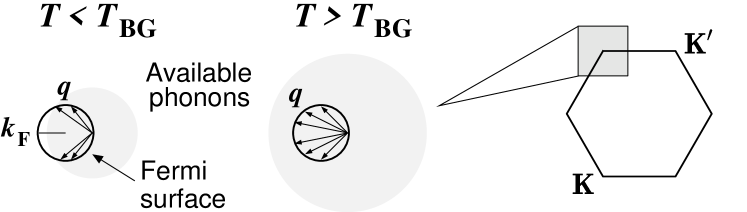
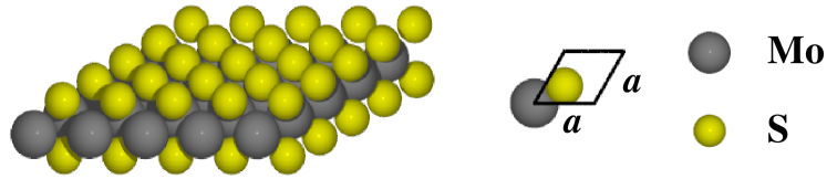
Figure 1: (Color online) Top: Illustration of acoustic phonon scattering in the $K,K^{\prime}$ valleys of the Brillouin zone showing the phase space available for scattering below and above the Bloch-Grüneisen temperature $T_{\text{BG}}$. The part of the hexagonal Brillouin zone marked by the gray-shaded box indicates the plotting range for the contour plots in Fig. 2. Bottom: Lattice and primitive unit cell of 2D hexagonal MoS₂.

In the present work, we study the acoustic phonon limited mobility of $n$-type 2D MoS₂ at low temperatures ($T<100$ K) taking into account both deformation potential (DP) and piezoelectric (PE) scattering. The flexural phonon couples weakly to charge carriers and is here neglected. In our previous work considering scattering of both acoustic and optical phonons Kaasbjerg et al. (2012a), only the deformation potential interaction was taken into account in the coupling to the acoustic phonons. There we found that the mobility at higher temperatures ($T>100$ K) was dominated by optical phonon scattering. With piezoelectric interaction included this is still the case, however, with a slightly lower room-temperature mobility of 320 cm² V^-1 s^-1 at $n=10^{11}$ cm^-2. Otherwise the conclusions of Ref. Kaasbjerg et al., 2012a remain unaffected. For the temperatures considered in this work, scattering by intervalley acoustic phonons and optical phonons is strongly suppressed and can be neglected Kaasbjerg et al. (2012a).

Using a first-principles approach, we calculate the deformation potential and piezoelectric interactions in 2D MoS₂. Supported by continuum model calculations of the acoustic el-ph interaction in 2D hexagonal lattices, this allows us to establish analytic expressions and the individual coupling strengths for the two scattering mechanisms. The calculated intrinsic low-temperature mobility provides a platform for comparison with future measurements of the carrier mobility in monolayer MoS₂ which can (i) lead to an experimental verification of the theoretical deformation potentials and piezoelectric constant reported here Kawamura and Das Sarma (1990), (ii) reveal to what extent the mobility is affected by extrinsic surface acoustic/optical phonons Knäbchen (1997); Mori and Ando (1989) which have turned out to be important in substrate-supported graphene samples Chen et al. (2008); Fratini and Guinea (2008); Konar et al. (2010); Zhang et al. (2013), and (iii) address the importance of the interplay between scattering of acoustic phonons and impurities which results in a complex temperature and density dependence of the mobility Min et al. (2012). In this context previous studies have emphasized the importance of including both the TA and LA phonon in order to obtain good agreement with experiment Stormer et al. (1990). With the present work we uncover new important aspects of the acoustic el-ph interaction and how it is affected by carrier screening. These are issues of high relevance for the understanding of acoustic phonon limited 2DEG mobilities in semiconductors and, in particular, monolayers of transition metal dichalcogenides.

The paper is organized as follows. Section II briefly summarizes the Boltzmann transport theory for acoustic phonon scattering. In Sec. III the first-principles results for the acoustic electron-phonon (el-ph) interaction are presented and the deformation potential and piezoelectric interactions are discussed in closer detail along with a microscopic description of carrier screening. Finally, the results for temperature and density dependence of the acoustic phonon limited mobility are presented in Sec. IV.

II Boltzmann Theory

Two-dimensional MoS₂ has a hexagonal lattice structure like graphene with the bottom of the conduction band residing in the $K,K^{\prime}$ points at the corners of the Brillouin zone Lebègue and Eriksson (2009); Cheiwchanchamnangij and Lambrecht (2012). The two $K,K^{\prime}$ valleys are perfectly isotropic with an effective electron mass of $m^{*}=0.48\;m_{e}$ Kaasbjerg et al. (2012a). The satellite valleys located at the $\Gamma$-$K$ path inside the Brillouin zone are well separated in energy from the $K,K^{\prime}$-valleys and therefore not important for the low-field transport properties Cheiwchanchamnangij and Lambrecht (2012); Kaasbjerg et al. (2012a). The conduction band spin splitting of a few meV due to the intrinsic spin-orbit interaction in 2D transition metal dichalcogenides Zhu et al. (2011); Cheiwchanchamnangij and Lambrecht (2012) can be safely neglected here. At the same time we note that a Rashba-type spin-orbit interaction can affect the phonon limited 2DEG mobility Chen et al. (2007); Biswas and Ghosh (2013).

In Boltzmann theory, the drift mobility $\mu_{xx}=\sigma_{xx}/ne$, where $\sigma_{xx}$ is the conductivity, is in the presence of (quasi) elastic scattering given by the Drude-like expression Kawamura and Das Sarma (1992)

$$\mu_{xx}=\frac{e\langle\tau_{k}\rangle}{m^{*}},$$ (2)

where $\tau_{k}$ is the energy-dependent relaxation time and the energy-weighted average $\langle\cdot\rangle$ is defined by

$$\langle A\rangle=\frac{1}{n}\int\!d\varepsilon_{\mathbf{k}}\;\rho(\varepsilon_{\mathbf{k}})\varepsilon_{\mathbf{k}}A(\varepsilon_{\mathbf{k}})\left(-\frac{\partial f}{\partial\varepsilon_{\mathbf{k}}}\right).$$ (3)

Here, $n$ is the two-dimensional carrier density, $\rho=g_{s}g_{v}m^{*}/2\pi\hbar^{2}$ is the density of states in 2D, $g_{s}=2$ and $g_{v}=2$ are the spin and valley degeneracy, respectively, $\varepsilon_{\mathbf{k}}=\hbar^{2}k^{2}/2m^{*}$ is the carrier energy, $f(\varepsilon_{\mathbf{k}})=\left\{1+\exp{[(\varepsilon_{\mathbf{k}}-\mu)/k_{\text{B}}T]}\right\}^{-1}$ is the equilibrium Fermi-Dirac distribution function, and $\mu$ is the chemical potential. For a degenerate electron gas, only scattering within a shell of width $k_{\text{B}}T$ around the Fermi level is relevant and $\mu_{xx}\approx e\tau_{k_{F}}/m^{*}$ applies.

In valley-degenerate semiconductors scattering in inequivalent valleys is not necessarily identical. In such cases the Boltzmann equation must be solved explicitly in all inequivalent valleys. In the absence of intervalley scattering this amounts to replacing the relaxation time in (2) with a valley-averaged relaxation time: $\tau=\sum_{v}\tau_{v}/N_{v}$, where $v$ denotes the valley index, $N_{v}$ is the number of inequivalent valleys, and $\tau_{v}$ denotes the individual valley relaxation times.

For acoustic phonon scattering, which to a good approximation can be treated as a quasielastic scattering process, the relaxation time for the individual acoustic phonons is given by Kawamura and Das Sarma (1992); Kaasbjerg et al. (2012a)

$$\frac{1}{\tau_{\lambda}(\varepsilon_{\mathbf{k}})}=\sum_{\mathbf{k}^{\prime}}\left(1-\cos{\theta_{\mathbf{k}\mathbf{k}^{\prime}}}\right)P_{\mathbf{k}\mathbf{k}^{\prime}}^{\lambda}\frac{1-f_{\mathbf{k}^{\prime}}}{1-f_{\mathbf{k}}},$$ (4)

where $\lambda$ denotes the branch index ($\lambda=$TA, LA), $\theta_{\mathbf{k}\mathbf{k}^{\prime}}$ is the scattering angle, and $f_{\mathbf{k}}=f(\varepsilon_{\mathbf{k}})$ is understood. The transition matrix element is given by

$$P_{\mathbf{k}\mathbf{k}^{\prime}}^{\lambda} =\frac{2\pi}{\hbar}\left|\frac{g_{\mathbf{k}\mathbf{q}}^{\lambda}}{\epsilon(q,T)}\right|^{2}\bigg{[}N_{\mathbf{q}\lambda}\delta(\varepsilon_{\mathbf{k}^{\prime}}-\varepsilon_{\mathbf{k}}-\hbar\omega_{\mathbf{q}\lambda})\bigg{.}$$

$$\quad+\bigg{.}\left(1+N_{\mathbf{q}\lambda}\right)\delta(\varepsilon_{\mathbf{k}^{\prime}}-\varepsilon_{\mathbf{k}}+\hbar\omega_{\mathbf{q}\lambda})\bigg{]},$$ (5)

where $\mathbf{q}=\mathbf{k}^{\prime}-\mathbf{k}$, $g_{\mathbf{k}\mathbf{q}}^{\lambda}$ is the el-ph coupling, $\epsilon(q,T)$ is the wave vector and temperature dependent static dielectric function of the 2DEG, and $\hbar\omega_{\mathbf{q}\lambda}=\hbar c_{\lambda}q$ is the acoustic phonon energy. The phonons are assumed to be in equilibrium and populated according to the Bose-Einstein distribution function $N_{\mathbf{q}\lambda}=N(\hbar\omega_{\mathbf{q}\lambda})$.

Screening of the el-ph interaction by the carriers themselves is accounted for by the dielectric function $\epsilon(q,T)$. As we here show, the presence of both normal and umklapp processes in the acoustic deformation potential interaction requires a microscopic description of carrier screening. The consequence of this is a central result of this work, and will be discussed in further detail in Sec. III.3.

In the present work the expression for the relaxation time in Eq. (4) is evaluated numerically assuming quasielastic scattering; i.e., the phonon energies are omitted in the $\delta$ functions of Eq. (II) (implying $q=2k\sin{\theta_{\mathbf{k}\mathbf{k}^{\prime}}/2}$) but included in the Fermi function $f_{\mathbf{k}^{\prime}}=f(\varepsilon_{\mathbf{k}}\pm\hbar\omega_{\mathbf{q}\lambda})$ of Eq. (4). This is particularly important in the BG regime where the phonon energy becomes comparable to the thermal smearing at the Fermi level; i.e., $\hbar\omega_{\mathbf{q}\lambda}\sim k_{\text{B}}T$.

III Interaction with acoustic phonons

In the following, we present first-principles calculations of the el-ph interaction in 2D MoS₂ obtained with the density-functional based method outlined in Ref. Kaasbjerg et al., 2012a and implemented in the GPAW electronic structure package Mortensen et al. (2005); Larsen et al. (2009); Enkovaara et al. (2010). As a complement to our first-principles calculations, we calculate in App. B the acoustic el-ph interaction in 2D materials using an elastic continuum model.

III.1 First-principles calculations

The interaction with the acoustic phonons can be written in the general form

$$g_{\mathbf{k}\mathbf{q}}^{\lambda}=\sqrt{\frac{\hbar}{2A\rho\omega_{\mathbf{q}\lambda}}}M_{\mathbf{k}\mathbf{q}}^{\lambda},$$ (6)

where $A$ is the area of the sample, $\rho$ is the mass density, $M_{\mathbf{k}\mathbf{q}}^{\lambda}=\langle\mathbf{k}+\mathbf{q}\rvert\delta V_{\mathbf{q}\lambda}\lvert\mathbf{k}\rangle$ is the matrix element between the Bloch states with wave vectors $\mathbf{k}$ and $\mathbf{k}+\mathbf{q}$, and $\delta V_{\mathbf{q}\lambda}$ is the change in the crystal potential due to a phonon with wave vector $\mathbf{q}$ and branch index $\lambda$. The couplings in the $K,K^{\prime}$ valleys are related through time-reversal symmetry as $\lvert M_{\mathbf{q}\lambda}^{K}\rvert=\lvert M_{-\mathbf{q}\lambda}^{K^{\prime}}\rvert$. As the hexagonal lattice of two-dimensional MoS₂ lacks a center of symmetry, charge carriers in monolayer MoS₂ interact with acoustic phonons through both the deformation potential and the piezoelectric interaction. The coupling matrix element therefore has contributions from both coupling mechanisms, i.e.

$$M_{\mathbf{q}\lambda}=M_{\mathbf{q}\lambda}^{\text{DP}}+M_{\mathbf{q}\lambda}^{\text{PE}}.$$ (7)

The two coupling mechanisms are often assumed to be out of phase, i.e. one is real and the other imaginary Mahan (2010) (see also App. B). This implies that piezoelectric and deformation potential interactions do not interfere in lowest-order perturbation theory, i.e. $\lvert M_{\mathbf{q}\lambda}\rvert^{2}=\lvert M_{\mathbf{q}\lambda}^{\text{DP}}+M_{\mathbf{q}\lambda}^{\text{PE}}\rvert^{2}=\lvert M_{\mathbf{q}\lambda}^{\text{DP}}\rvert^{2}+\lvert M_{\mathbf{q}\lambda}^{\text{PE}}\rvert^{2}$, and can therefore be treated as separate scattering mechanisms.

Deformation potential interaction

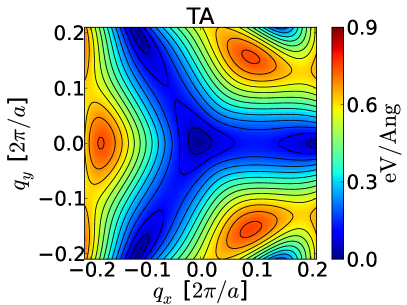
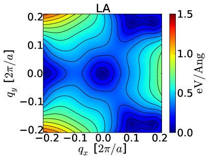
Piezoelectric interaction

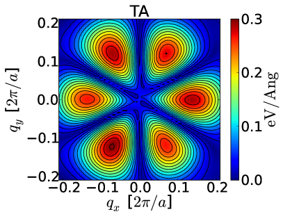
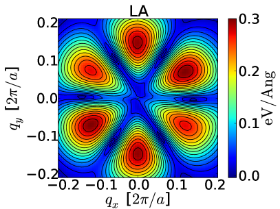
Relative phase $\lvert\phi\rvert$

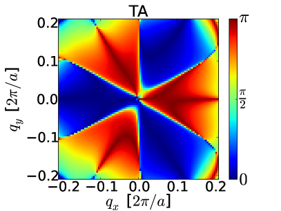
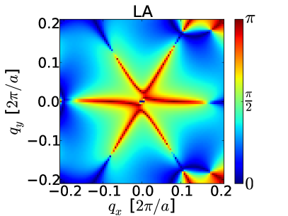
Figure 2: (Color online) Calculated deformation potential and piezoelectric interactions in the $K$-valley of the conduction band in monolayer MoS₂. The contour plots show the absolute value of the calculated coupling matrix elements $M_{\mathbf{q}\lambda}^{\text{DP/PE}}$ at $\mathbf{k}=\mathbf{K}$ for the TA (left) and LA (right) phonons as a function of the two-dimensional phonon wave vector $\mathbf{q}$. The absolute value of the relative phase $\phi$ between the two interactions (see Eq. (8)) is shown in the bottom plots.

In Fig. 2 we show our first-principles results for the deformation potential and piezoelectric interactions with the TA and LA phonons in 2D MoS₂ for $\mathbf{k}=\mathbf{K}$ foo (b). The two coupling mechanisms have been obtained from the total coupling matrix element in Eq. (7) using the real-space partitioning scheme outlined in App. C.1. The scheme is based on the observation that the deformation potential is short range while the piezoelectric interaction is long range, and can therefore be separated in real space. While the deformation potential couplings have the three fold rotational symmetry of the conduction band in the vicinity of the $K,K^{\prime}$ points, the six-fold rotational symmetry of the piezoelectric couplings stems from the hexagonal crystal lattice.

The interference between the deformation potential and piezoelectric interaction can be inferred from the relative phase $\phi$ between their complex-valued matrix elements,

$$\phi=\text{Im}[\ln{(M_{\mathbf{q}\lambda}^{\text{PE}}/M_{\mathbf{q}\lambda}^{\text{DP}})}].$$ (8)

The absolute value of the relative phase is shown in the bottom row of Fig. 2. At long wavelengths, we find that the above-mentioned out-of-phase property ($\phi=\pi/2$) holds for the LA phonon only. For the TA phonon the two coupling mechanisms interfere ($\phi=0,\pi$) and must hence be considered together. Deviations from this behavior occur at short wavelengths where the strictly transverse and longitudinal character of the TA and LA phonons vanishes. However, for long-wavelength acoustic phonon scattering, the interaction with the TA and LA phonons is given by fully interfering and noninterfering couplings, respectively.

III.1.1 Normal and umklapp contributions

In order to gain further understanding of the deformation potential interaction, we here quantify the contributions from normal and umklapp processes. Formally, the two are associated with terms in the Fourier expansion of the short-range phonon-induced change in the crystal potential,

$$\delta V_{\mathbf{q}\lambda}(\mathbf{r})=\sum_{\mathbf{G}}e^{i(\mathbf{q}+\mathbf{G})\cdot\mathbf{r}}\delta V_{\mathbf{q}+\mathbf{G}}^{\lambda},$$ (9)

with $\mathbf{G}=\mathbf{0}$ and $\mathbf{G}\neq\mathbf{0}$ for normal and umklapp processes, respectively ($\mathbf{G}$ is a reciprocal lattice vector, see also App. C.2). Since the coupling to the TA phonon vanishes when umklapp processes are neglected altogether Madelung (1996), they are essential for a correct description of the acoustic el-ph interaction.

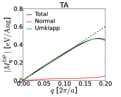
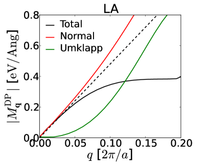
Figure 3: (Color online) Normal and umklapp contributions to the deformation potential interaction for the TA (left) and LA (right) phonon. The plots show the angular average of the deformation potential interactions in Fig. 2 and their contributions from normal and umklapp processes given by Eq. (10) (full lines). The dashed lines show the analytic deformation potential interaction in Eq. (11).

In Fig. 3 we show the normal and umklapp contributions to the acoustic deformation potential interactions obtained with the Fourier filtering method outlined in App. C.2. The plots show the absolute value of the $\mathbf{q}$-direction average of the matrix element

$$M_{\mathbf{q}\lambda}^{\text{DP},X}=\langle\mathbf{k}+\mathbf{q}\rvert\delta V_{\mathbf{q}\lambda}^{X}\lvert\mathbf{k}\rangle,\quad X=N,U,$$ (10)

where $\delta V_{\mathbf{q}\lambda}^{X}$ denotes the phonon-induced potential with normal ($N$) and umklapp ($U$) processes included, respectively. Due to the complex-valued matrix elements, the absolute values of the normal and umklapp contributions do not add up to the total matrix element. In accordance with the statement below Eq. (9), we find that in the long-wavelength limit the deformation potential interactions for the TA and LA phonons are completely dominated by umklapp and normal processes, respectively. At shorter wavelengths both processes contribute.

The separation of the deformation potential interaction into contributions from normal and umklapp processes is not only of technical character. As we show below in Sec. III.3, it has important consequences for the screening of the deformation potential interaction.

III.2 Analytic expressions for the acoustic el-ph interaction

In the following, the analytic expressions for the deformation potential and piezoelectric couplings obtained in App. B are introduced and the coupling strengths are determined from the first-principles el-ph couplings.

III.2.1 Deformation potential interaction

The deformation potential originates from the local changes of the crystal potential caused by the atomic displacements due to an acoustic phonon. The determination of the interaction strength thus requires a microscopic calculation, such as the first-principles approach used in this work.

The interaction with acoustic phonons via the deformation potential interaction is most commonly assumed to be isotropic and linear in the phonon wave vector, i.e.

$$\lvert M_{\mathbf{q}\lambda}^{\text{DP}}\rvert=\Xi_{\lambda}q,$$ (11)

where $\Xi_{\lambda}$ is the acoustic deformation potential Mahan (2010). Since the true deformation potential couplings in Fig. 2 are anisotropic and show a more complex $q$-dependence at shorter wavelengths, the deformation potential of Eq. (11) must be regarded as an effective coupling parameter. In valley-degenerate semiconductors where the couplings in the different valleys are related through time-reversal symmetry, the effective deformation potential furthermore accounts for the variation in the angular dependence of the coupling between inequivalent valleys. We have here recalculated the acoustic deformation potentials from Ref. Kaasbjerg et al., 2012a in order to avoid undesired contributions from the piezoelectric interaction that potentially were included there. The new deformation potentials are given in Tab. 1 and the couplings are shown in Fig. 3 (dashed lines) together with the angular average of the first-principles couplings.

For deformation potential scattering above the BG temperature where the equipartition approximation $N_{\mathbf{q}}\sim k_{\text{B}}T/\hbar\omega_{\mathbf{q}}\gg 1$ applies and with screening neglected, the relaxation time in Eq. (4) becomes independent of the carrier energy and is given by Kaasbjerg et al. (2012a)

$$\frac{1}{\tau_{\lambda}(\varepsilon_{\mathbf{k}})}=\frac{m^{*}\Xi_{\lambda}^{2}k_{\text{B}}T}{\hbar^{3}\rho c_{\lambda}^{2}}.$$ (12)

This results in a $\mu\sim T^{-1}$ temperature dependence of the 2DEG mobility characteristic of acoustic deformation potential scattering in the high-temperature regime.

III.2.2 Piezoelectric interaction

Piezoelectric coupling to acoustic phonons occurs in crystals lacking an inversion center and originates from the macroscopic polarization that accompanies an applied strain $\epsilon_{ij}$. The strength of the interaction is given by the piezoelectric tensor $e_{ij}$ here given in Voigt notation.

Table 1: Material parameters for monolayer MoS₂ used in the present work. Apart from the acoustic deformation potentials and the piezoelectric constant all parameters have been adopted from Ref. Kaasbjerg et al., 2012a.

Parameter	Symbol	Value
Lattice constant	$a$	3.14 Å
Ion mass density	$\rho$	$3.1\times 10^{-7}$ g/cm2
Effective electron mass	$m^{*}$	0.48 $m_{e}$
Transverse sound velocity	$c_{\text{TA}}$	$4.2\times 10^{3}$ m/s
Longitudinal sound velocity	$c_{\text{LA}}$	$6.7\times 10^{3}$ m/s
Acoustic deformation potentials
TA	$\Xi_{\text{TA}}$	$1.5$ eV
LA	$\Xi_{\text{LA}}$	$2.4$ eV
Piezoelectric constant	$e_{11}$	$3.0\times 10^{-11}$ C/m
Effective layer thickness	$\sigma$	5.41 Å

In App. B.2 we obtain the piezoelectric interaction in a 2D hexagonal lattice using continuum theory. We find that the piezoelectric interaction is given by

$$\lvert M_{\mathbf{q}\lambda}^{\text{PE}}\rvert=\frac{e_{11}e}{\epsilon_{0}}q\times\text{erfc}(q\sigma/2)\lvert A_{\lambda}(\hat{\mathbf{q}})\rvert,$$ (13)

where $e_{11}$ (units of C/m) is the only independent component of the piezoelectric tensor of the 2D hexagonal lattice Sai and Mele (2003), $\epsilon_{0}$ is the vacuum permeability, erfc is the complementary error function, $\sigma$ is an effective width of the electronic wave functions, and $A_{\lambda}(\hat{\mathbf{q}})$ is an anisotropy factor that accounts for the angular dependence of the piezoelectric interaction. It is given by

$$A_{\text{TA}}(\hat{\mathbf{q}})=-\sin{3\theta_{\mathbf{q}}}\quad\text{and}\quad A_{\text{LA}}(\hat{\mathbf{q}})=\cos{3\theta_{\mathbf{q}}}$$ (14)

for the TA and LA phonon, respectively, and results in a highly anisotropic piezoelectric interaction.

The first-principles results for the piezoelectric interaction in Fig. 2 are in overall good agreement with the analytic expression in Eq. (13) (see also Figs. 8 and 10) foo (c). From a fit to the first-principles results, the piezoelectric constant of 2D MoS₂ is estimated to be $e_{11}\sim 3.0\times 10^{-11}$ C/m ($\sim$0.01 $e$/bohr). This is an order of magnitude smaller than a recently reported value ($e_{11}=3.06\times 10^{-10}$) obtained with a Berry’s phase approach Duerloo et al. (2012). We are at present, however, not able to clarify the origin of this disagreement.

The $q$-dependence of the 2D piezoelectric interaction in Eq. (13) is qualitatively different from the one in 3D bulk systems where $M_{\mathbf{q}\lambda}^{\text{PE}}\sim\text{constant}$ Mahan (2010). In the long-wavelength limit where $\text{erfc}(q\sigma/2)\sim 1-q\sigma/\sqrt{2\pi}$, the 2D piezoelectric interaction acquires a linear $q$-dependence $M_{\mathbf{q}\lambda}^{\text{PE}}\sim q$. Hence, the deformation potential and piezoelectric interaction in a 2D lattice behave qualitatively the same in the long-wavelength limit. Assuming that the linear long-wavelength behavior holds, the high-temperature relaxation time for piezoelectric scattering is given by Eq. (12) with the replacement

$$\Xi_{\lambda}^{2}\rightarrow\frac{1}{2}\left(\frac{e_{11}e}{\epsilon_{0}}\right)^{2},$$ (15)

where the factor $1/2=\langle A_{\lambda}^{2}\rangle$ stems from the angular mean of the piezoelectric interaction foo (d). This corresponds to an effective isotropic piezoelectric coupling with $A_{\lambda}(\hat{\mathbf{q}})=1/\sqrt{2}$ in Eq. (13). The relative strength of the deformation potential and piezoelectric interactions is thus governed by the ratio $(e_{11}e/\epsilon_{0})/\Xi_{\lambda}$ of the prefactors in Eqs. (11) and (13). Since this is of the order of unity with the parameters for 2D MoS₂ listed in Table 1, both coupling mechanisms must be taken into account.

III.3 Screening of the acoustic el-ph interaction

The first-principles el-ph interactions presented above have been obtained for the neutral material and therefore do not take into account screening by the 2DEG in extrinsic 2D MoS₂. In the following we apply a microscopic theory for carrier screening and show that the normal and umklapp contributions to the deformation potential interaction are screened differently.

Formally, the screened el-ph interaction can be obtained by replacing the phonon-induced potential $\delta V_{\mathbf{q}\lambda}$ in the matrix element $M_{\mathbf{k}\mathbf{q}}^{\lambda}$ of Eq. (6) with its screened counterpart

$$\delta V^{\text{scr}}_{\mathbf{q}\lambda}(\mathbf{r})=\int\!d\mathbf{r}^{\prime}\,\epsilon^{-1}(\mathbf{r},\mathbf{r}^{\prime})\delta V_{\mathbf{q}\lambda}(\mathbf{r}^{\prime}),$$ (16)

where $\epsilon^{-1}$ is the (static) microscopic dielectric function of the 2DEG. Inserting (9), this can be recast in Fourier space in terms of the $\mathbf{q}$-dependent dielectric matrix $\epsilon_{\mathbf{G}\mathbf{G}^{\prime}}^{-1}$ Hybertsen and Louie (1987) as

$$\delta V_{\mathbf{q}\lambda}^{\text{scr}}(\mathbf{r}) =\sum_{\mathbf{G}}e^{i(\mathbf{q}+\mathbf{G})\cdot\mathbf{r}}\sum_{\mathbf{G}^{\prime}}\epsilon_{\mathbf{G}\mathbf{G}^{\prime}}^{-1}(\mathbf{q})\delta V_{\mathbf{q}+\mathbf{G}^{\prime}}^{\lambda}$$

$$\simeq\sum_{\mathbf{G}}e^{i(\mathbf{q}+\mathbf{G})\cdot\mathbf{r}}\epsilon_{\mathbf{G}\mathbf{G}}^{-1}(\mathbf{q})\delta V_{\mathbf{q}+\mathbf{G}}^{\lambda},$$ (17)

where $\mathbf{G}$ and $\mathbf{G}^{\prime}$ are reciprocal lattice vectors and the second equality holds in the diagonal approximation $\epsilon_{\mathbf{G}\mathbf{G}^{\prime}}^{-1}=\delta_{\mathbf{G}\mathbf{G}^{\prime}}\epsilon_{\mathbf{G}\mathbf{G}}^{-1}$. To a good approximation, the screened phonon-induced potential thus follows by dividing the individual Fourier components in Eq. (9) by the components $\epsilon_{\mathbf{G}\mathbf{G}}$ of the diagonal dielectric matrix. The latter is related to the 2DEG polarizability $\chi^{0}_{\mathbf{G}\mathbf{G}}(\mathbf{q})$ through the expression Hybertsen and Louie (1987)

$$\epsilon_{\mathbf{G}\mathbf{G}}(\mathbf{q})=1-\frac{e^{2}}{2\epsilon_{0}\lvert\mathbf{q}+\mathbf{G}\rvert}\chi^{0}_{\mathbf{G}\mathbf{G}}(\mathbf{q}),$$ (18)

which is similar to the standard long-wavelength expression for the dielectric function in Eq. (19), however, with the important difference that the denominator in the second term of Eq. (18) contains a factor $\lvert\mathbf{q}+\mathbf{G}\rvert$ instead of a factor $q$. For intravalley scattering where $q\ll\lvert\mathbf{G}\rvert$, this implies that $\epsilon_{\mathbf{G}\mathbf{G}}(\mathbf{q})$ behaves differently at long ($\mathbf{G}=\mathbf{0}$) and short ($\mathbf{G}\neq\mathbf{0}$) wavelengths; while it diverges as $1/q$ in the $q\rightarrow 0$ limit in the former case, it approaches a finite value in the latter. As an immediate consequence, normal and umklapp components of the el-ph interaction are renormalized differently with a significantly stronger screening of the former.

While a correct description of the screened el-ph interaction can only be obtained from Eq. (III.3), the calculation of the microscopic dielectric function from first principles is, however, beyond the scope of the present study. Instead, we adopt the following ad hoc approach to carrier screening.

III.3.1 Effective screening scheme

In order to account for the qualitative difference between the screening of normal and umklapp processes, the dielectric function of the 2DEG in Eq. (18) is approximated as follows.

For the long-wavelength component ($\mathbf{G}=\mathbf{0}$) of the dielectric function, well-established approximations exist in the literature Ando et al. (1982). We here apply the finite-temperature RPA theory due to Maldague Maldague (1978),

$$\epsilon(q,T,\mu)=1-\frac{e^{2}}{2\epsilon_{0}q}\chi^{0}(q,T,\mu),$$ (19)

where $\mu$ is the chemical potential and the static polarizability at finite temperatures is obtained as

$$\chi^{0}(q,T,\mu)=\int_{0}^{\infty}\!d\mu^{\prime}\,\frac{\chi^{0}(q,0,\mu^{\prime})}{4k_{\text{B}}T\cosh^{2}{\frac{\mu-\mu^{\prime}}{2k_{\text{B}}T}}}.$$ (20)

Here, $\chi^{0}(q,0,\mu)$ is the zero-temperature RPA polarizability given by the density of states $\chi^{0}(q,0,\mu)=-\rho$ for $q<2k_{F}$ (see also App. A) Ando et al. (1982). The integral in Eq. (20) is evaluated numerically using the approach of Ref. Flensberg and Hu, 1995. We have here neglected the form factor in the polarizability arising from the finite thickness of the electronic Bloch functions. First-principles calculations of the RPA dielectric function (see e.g. Refs. Hybertsen and Louie, 1987; Yan et al., 2011) could be helpful in clarifying to which extent this leads to an overestimation of the screening strength.

For the short-wavelength part ($\mathbf{G}\neq\mathbf{0}$) of the dielectric function, we introduce an effective dielectric constant $\epsilon_{\text{eff}}$ which acts as a simple scaling parameter for the $\mathbf{G}\neq\mathbf{0}$ components of the potential in Eq. (III.3). From the relations $\lvert\mathbf{G}\rvert\gtrsim q_{\text{TF}}\gg e^{2}/2\epsilon_{0}\lvert\chi^{0}_{\mathbf{G}\mathbf{G}}\rvert$, where $q_{\text{TF}}$ is the Thomas-Fermi screening wave vector (see App. A) and the latter inequality follows from the expression for the microscopic polarizability Hybertsen and Louie (1987), we observe that the short-wavelength screening efficiency is relatively weak; i.e. $\epsilon_{\mathbf{G}\mathbf{G}}\sim 1$. We can hence to a good approximation set $\epsilon_{\text{eff}}=1$ thus leaving the umklapp contribution to the deformation potential interaction unscreened.

III.3.2 Total screened el-ph couplings

With our findings above, the screened matrix element for the acoustic el-ph interaction can be written as

$$M_{\mathbf{q}\lambda}^{\text{scr}}(n,T)=\frac{M_{\mathbf{q}\lambda}^{\text{DP},N}}{\epsilon(q,T,\mu)}+\frac{M_{\mathbf{q}\lambda}^{\text{DP},U}}{\epsilon_{\text{eff}}}+\frac{M_{\mathbf{q}\lambda}^{\text{PE}}}{\epsilon(q,T,\mu)}.$$ (21)

Here, the normal contribution to the deformation potential interaction and the long-range piezoelectric interaction are screened by the long-wavelength dielectric function in Eq. (19), while the umklapp contribution to the deformation potential interaction is screened by $\epsilon_{\text{eff}}$. It should be noted that this differs from conventional descriptions of the screened acoustic el-ph interaction where the deformation potential interaction is either screened with a long-wavelength dielectric function or left unscreened (see e.g. Refs. Walukiewicz et al., 1984; Kawamura and Das Sarma, 1992).

As the deformation potential interactions for the TA and LA phonons are largely dominated by umklapp and normal processes, they can to a good approximation be screened by $\epsilon_{\text{eff}}$ and $\epsilon$ in Eq. (19), respectively, thus leaving the deformation potential interaction for the TA phonon unscreened. Taking into account the interference between the deformation potential and piezoelectric interaction, we can hence approximate the coupling matrix elements for the TA and LA phonon as

$$M_{\mathbf{q}\text{TA}}^{\text{scr}}(n,T)\approx\frac{M_{\mathbf{q}\text{TA}}^{\text{DP}}}{\epsilon_{\text{eff}}}+\frac{M_{\mathbf{q}\text{TA}}^{\text{PE}}}{\epsilon(q,T,\mu)}$$ (22)

and

$$M_{\mathbf{q}\text{LA}}^{\text{scr}}(n,T)\approx i\frac{M_{\mathbf{q}\text{LA}}^{\text{DP}}}{\epsilon(q,T,\mu)}+\frac{M_{\mathbf{q}\text{LA}}^{\text{PE}}}{\epsilon(q,T,\mu)},$$ (23)

respectively, where $M_{\mathbf{q}\lambda}^{\text{DP/PE}}$ are given by Eqs. (11) and (13).

III.3.3 Efficiency of long-wavelength screening

In the following we provide a qualitative estimate of the efficiency of long-wavelength carrier screening given by the dielectric function in Eq. (19). The screening strength is in this case governed by the dimensionless parameter

$$q_{s}(T)=\frac{q_{\text{TF}}(T)}{{\tilde{q}}(T)},$$ (24)

where $q_{\text{TF}}(T)$ is the finite-temperature Thomas-Fermi wave vector and $\tilde{q}$ denotes a typical scattering wave vector. In the case of acoustic phonon scattering $\tilde{q}$ is given by

$$\tilde{q}=\bigg{\{}\begin{array}[]{l}\mathrm{min}(k_{F},q_{\text{th}}),\quad T\lesssim T_{F}\\ \mathrm{min}(k_{\text{avg}},q_{\text{th}}),\quad T\gtrsim T_{F},\end{array}$$ (25)

in the degenerate ($T\lesssim T_{F}$) and nondegenerate ($T\gtrsim T_{F}$) regime, respectively, and where $T_{F}$ is the Fermi temperature. Here $q_{\text{th}}=k_{\text{B}}T/2\hbar c_{\text{ph}}$ is a typical scattering wave vector in the BG regime where the accessible phase space is restricted by the availability of thermally excited phonons. Above the BG temperature where scattering on the full Fermi surface is possible, $k_{F}$ becomes a typical scattering wave vector. In the case of a nondegenerate 2DEG where the average carrier energy is $\langle\varepsilon_{\mathbf{k}}\rangle=k_{\text{B}}T$, $k_{\text{avg}}=\sqrt{2m^{*}k_{\text{B}}T/\hbar^{2}}$ is a typical wave vector.

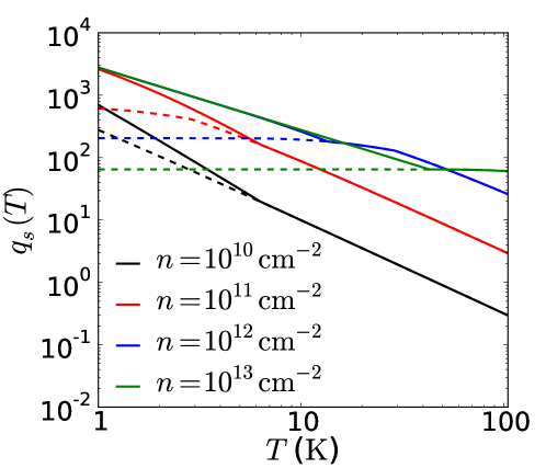
Figure 4: (Color online) Temperature and density dependence of the dimensionless screening parameter $q_{s}(T)$ in Eq. (24) for acoustic phonon (full lines) and charged impurity (dashed lines) scattering in 2D MoS₂.

In the low-temperature limit, the screening parameter for acoustic phonon scattering is given by

$$q_{s}(T\rightarrow 0)\approx\frac{q_{\text{TF}}}{q_{\text{th}}}=\frac{g_{s}g_{v}e^{2}m^{*}c_{\text{ph}}}{2\pi\epsilon_{0}\hbar k_{\text{B}}T},$$ (26)

which is independent of the carrier density. The $T^{-1}$ divergence of the low-temperature screening parameter implies that scattering of acoustic phonons via normal process deformation potential and piezoelectric interaction is strongly suppressed for a degenerate 2DEG in the BG regime.

It is interesting to compare this with the screening parameter for charged impurity scattering. In this case, scattering on the full Fermi surface is possible at low temperatures. Hence, $\tilde{q}=k_{F/\text{avg}}$ in the degenerate/nondegenerate regime and the low-temperature limit of the screening parameter becomes

$$q_{s}(T\rightarrow 0)\approx\frac{q_{\text{TF}}}{k_{F}}=\frac{(g_{s}g_{v})^{3/2}e^{2}m^{*}}{4\pi\epsilon_{0}\hbar^{2}\sqrt{4\pi n}},$$ (27)

which is independent of temperature and decreases with the carrier density. This results in a less efficient screening of impurity scattering compared to acoustic phonon scattering at high densities and low temperatures.

The full temperature dependence of the screening parameter for scattering of acoustic phonons (full lines) and impurities (dashed lines) is shown in Fig. 4 for different carrier densities and $c_{\text{ph}}=5\times 10^{3}$ m/s representative of the acoustic sound velocities in 2D MoS₂. In the low temperature regime, the limits in Eqs. (26) and (27) are approached. Due to the density and temperature dependence of the Debye-Hückel wave vector, $q_{\text{D}}\propto n/k_{\text{B}}T$, the screening strength becomes independent of the scattering mechanism and increases (decreases) with the carrier density (temperature) in the nondegenerate high-temperature regime.

The overall large values of the screening parameter ($q_{s}(T)\gg 1$) in Fig. 4 follow from a large effective mass and valley degeneracy. Carrier screening in monolayer MoS₂ and other 2D transition metal dichalcogenides is therefore inherently strong and the screening strength exceeds that of e.g. Si and GaAs based 2DEGs Das Sarma et al. (2011). For scattering of acoustic phonons this has the important consequence that normal process deformation potential and piezoelectric interaction is strongly reduced already at relative low carrier densities $n\gtrsim 10^{11}$ cm^-2.

IV Results

In the following we use the Boltzmann equation approach outlined in Section II to study the temperature and density dependence of the acoustic phonon limited mobility in 2D MoS₂ for temperatures $T<100$ K and high carrier densities $10^{10}$ to $3\times 10^{13}$ cm^-2. The mobility limited by scattering of acoustic phonons follows a generic temperature dependence $\mu\sim T^{-\gamma}$ where the exponent $\gamma$ depends on temperature, carrier density, and the dominating scattering mechanism. The same holds for the resistivity $\rho=(ne\mu)^{-1}$ with a change in the sign of the exponent.

In order to establish the relative strength of deformation potential and piezoelectric scattering in 2D MoS₂, we start by considering the scattering rate given by the expression for the inverse relaxation time in Eq. (4) with the replacement $(1-\cos{\theta_{\mathbf{k}\mathbf{k}^{\prime}}})\rightarrow 1$. Figure 5 shows energy dependence of the individual scattering rates due to deformation potential (dashed lines) and piezoelectric (full lines) scattering for carrier densities $n=10^{11}$ cm^-2 (left) and $n=10^{13}$ cm^-2 (right) and temperatures $T=10$ K and $T=50$ K. With the Fermi temperature given by $T_{F}\approx 29\,\tilde{n}$ K ($E_{F}\approx 2.5\,\tilde{n}$ meV), the two plots correspond to a nondegenerate and degenerate carrier distribution, respectively. The BG temperatures for the TA and LA phonons are in the two plots: (left) $<10$ K, and (right) $\sim$36 K and $\sim$57 K, respectively.

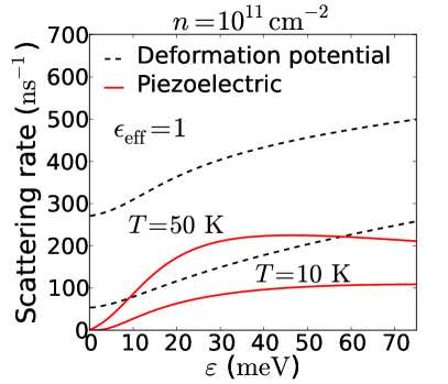
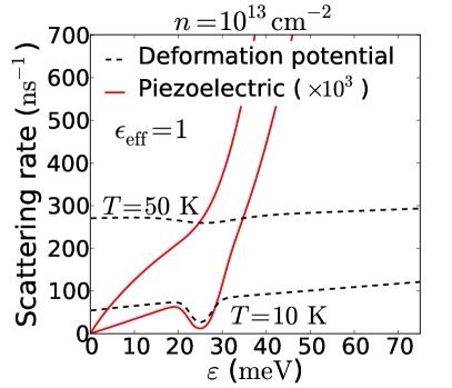
Figure 5: (Color online) Scattering rate for deformation potential (dashed lines) and piezoelectric (full lines) interaction in 2D MoS₂ at temperatures $T=10$ K and $T=50$ K and carrier densities $n=10^{11}$ cm^-2 (left) and $n=10^{13}$ cm^-2 (right). This corresponds to Fermi energies of $E_{F}\approx 0.25$ meV and $E_{F}\approx 25$ meV, respectively. In the right plot, the BG temperature is $T_{\text{BG}}\approx 36$ $(57)$ K for the TA (LA) phonon. At $T=10$ K, the dip in the scattering rate that appears at the Fermi energy is a clear fingerprint of Bloch-Grüneisen physics.

In the nondegenerate regime shown in the left plot of Fig. 5, carrier screening is weak implying that deformation potential and piezoelectric scattering are of the same order of magnitude. At low energies, however, deformation potential scattering of the LA phonon and piezoelectric scattering are strongly screened and unscreened deformation potential scattering of the TA phonon dominates the scattering rate. The saturation of the piezoelectric scattering rate at high energies is a consequence of the nonmonotonic $q$-dependence of the matrix element in Eq. (13) (see also Fig. 10).

In the degenerate high-density regime shown in the right plot of Fig. 5, carrier screening is so strong that the piezoelectric scattering rate is diminished by almost three orders of magnitude relative to the low-density scattering rate (note the scaling factor in the legend of the right plot in Fig. 5). In this regime, unscreened deformation potential scattering of the TA phonon therefore completely dominates. The dip in the scattering rate that develops at the Fermi level with decreasing temperature is a signature of transport in the BG regime. In this temperature regime the freezing out of short-wavelength acoustic phonons and the sharpening of the Fermi surface strongly limit the phase space available for acoustic phonon scattering resulting in a strong suppression of scattering at the Fermi level.

Next, we consider the temperature and density dependence of the mobility. Due to the strong anisotropy of the piezoelectric interaction, the mobility in 2D MoS₂ is slightly anisotropic. Along the different high-symmetry directions of the hexagonal lattice we find that the variation in the mobility is less than $\sim$10%. In the following we shall focus on a single direction of the applied electric field foo (e).

The temperature dependence of the mobility is shown in Fig. 6 for carrier densities $10^{10}$ to $3\times 10^{13}$ cm^-2 corresponding to BG temperatures up to $\sim$62 K ($\sim$99 K) for the TA (LA) phonon. Both the mobility (upper) and the exponent $\gamma=-d\log{\mu}/d\log{T}$ (lower) of its power-law dependence $\mu\sim T^{-\gamma}$ are shown. At the lowest densities the characteristic temperatures $T_{\text{BG}}$ and $T_{F}$ are comparable while $T_{F}>T_{\text{BG}}$ for $n\gtrsim 10^{12}$ cm^-2. As a consequence, the crossover to the high-mobility BG regime at $T\sim T_{\text{BG}}$, marked by the dots in the lower plot, appears clearly for all carrier densities.

In the high-temperature regime $T\gtrsim T_{\text{BG}}$, the mobility shows an approximate linear temperature dependence with $1\lesssim\gamma\lesssim 1.5$. This is in good agreement with the individual high-temperature limits for unscreened deformation potential and piezoelectric scattering which we find to be $\gamma=1$ and $\gamma\lesssim 1$, respectively. At the lowest carrier densities, the larger value of $\gamma\sim 1.5$ appearing at $T>T_{\text{BG}}$ originates from the temperature dependence of the dielectric function for a nondegenerate carrier distribution.

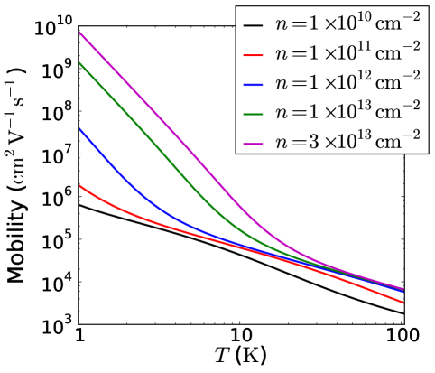
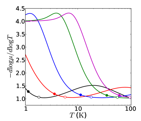
Figure 6: (Color online) Acoustic phonon limited mobility vs temperature. Top: Mobility vs temperature for different carrier densities. Bottom: Temperature dependence of the exponent $\gamma$ in $\mu\sim T^{-\gamma}$ for the same set of carrier densities. The dots mark the BG temperatures of the TA ($\bullet$) and LA ($\circ$) phonons, respectively.

In the low-temperature BG regime $T<T_{\text{BG}}$, a stronger temperature dependence with $1<\gamma\lesssim 4$ appears and the mobility approaches a $\mu\sim T^{-4}$ limiting behavior at $T\ll T_{\text{BG}}$. Numerically, we find that the $\gamma=4$ limiting behavior is characteristic of unscreened deformation potential scattering. Screened deformation potential and piezoelectric scattering share the same $\gamma=6$ limit due the identical long-wavelength limits of their respective couplings in Eqs. (11) and (13). The mobility at $T\ll T_{\text{BG}}$ is thus completely dominated by unscreened deformation potential scattering of the TA phonon. Our findings for the low-temperature limits of the mobility due to scattering of 2D phonons differ from the usual low-temperature limits of the 2DEG mobility with scattering of bulk 3D phonons in heterostructures. In this case, the limits are given by $\gamma=5$ for unscreened deformation potential scattering and $\gamma=7$ and $\gamma=5$ for screened deformation potential and piezoelectric scattering, respectively Price (1984); Stormer et al. (1990). As the low-temperature limits of the mobility are only realized deep inside the BG regime $T\ll T_{\text{BG}}$, they may, however, be difficult to observe experimentally.

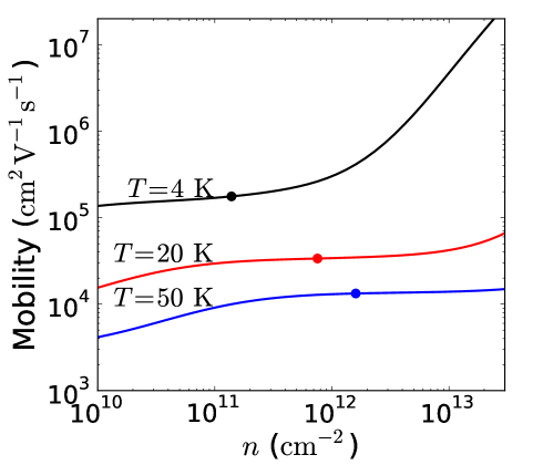
Figure 7: (Color online) Acoustic phonon limited mobility vs carrier density for temperatures $T=4$, 20, 50 K. The dots mark the quantum-classical crossover from a nondegenerate to a degenerate carrier distribution at $T=T_{F}$.

In Fig. 7 we show the calculated density dependence of the mobility for temperatures $T=4$, 20, 50 K. In the nondegenerate low-density regime, the density dependence of Debye-Hückel screening results in a mobility that increases with the density. For the lowest temperature where carrier screening becomes strong, unscreened deformation potential scattering of the TA phonon dominates the mobility resulting in a weaker density dependence. The same holds for densities in the vicinity of the quantum-classical crossover at $T\sim T_{F}$ (marked by dots in Fig. 7) where the mobility shows almost no density dependence. In the degenerate high-density regime, the mobility approaches a $\mu\sim n^{1.5}$ behavior at low temperatures. The strong density dependence of the mobility in this regime can be ascribed to two factors: (i) a Fermi velocity that increases with the carrier density as $v_{F}\sim\sqrt{n}$, and (ii) transport in the Bloch-Grüneisen regime where the scattering rate for fixed temperature $T$ decreases with the density. The latter is a consequence of a reduction in the fraction of the Fermi surface that is probed by acoustic phonon scattering when the density (Fermi wave vector) increases.

We end by briefly commenting on the applicability of the expression $1/\mu=1/\mu_{0}+\alpha T$ often used to fit experimental mobilities Stormer et al. (1990); Kawamura and Das Sarma (1990, 1992) in the linear high-temperature regime. Here, $\mu_{0}$ is the residual mobility due to e.g. impurity scattering and $\alpha$ is the density-dependent slope of the linear temperature dependence. In Fig. 6 it is seen to apply at $T>T_{\text{BG}}$ except for the lowest densities where the inverse mobility becomes slightly nonlinear. From the density dependence of the mobility in Fig. 7 we conclude that the temperature coefficient $\alpha$ is a monotonically decreasing function of the carrier density.

V Conclusions

In this work we have combined analytic and first-principles calculations of the el-ph interaction with an semianalytic solution of the Boltzmann equation to study the temperature and density dependence of the acoustic phonon limited mobility in 2D $n$-type MoS₂. The acoustic deformation potentials for the TA and LA phonons and the piezoelectric constant in 2D MoS₂ were extracted from the first-principles el-ph interaction and from a microscopic description of carrier screening it was shown that the umklapp contribution to the deformation potential interaction is not affected by screening.

Due to strong screening of deformation potential scattering of the LA phonon and piezoelectric scattering of both the TA and LA phonon, the mobility was found to be dominated by unscreened deformation potential scattering of the TA phonon at high densities. At low carrier densities $10^{10}$–$10^{11}$ cm^-2 deformation potential and piezoelectric scattering were found to be comparable. For $T<10$ K and moderate to high carrier densities $n\gtrsim 10^{11}$ cm^-2, intrinsic mobilities in excess of $~{}10^{5}$ cm² V^-1 s^-1 were predicted. At temperatures $T\sim 100$ K, the acoustic phonon limited mobility does not exceed $\sim 7\times 10^{3}$ cm² V^-1 s^-1. In the low-temperature BG regime $T\ll T_{\text{BG}}$, the mobility acquires a $\mu\sim T^{-4}$ dependence characteristic of unscreened deformation potential scattering of 2D phonons. The mobility was furthermore found to increase monotonically with the carrier density. Similar conclusions can be expected to hold for monolayers of other transition metal dichalcogenides which have similar atomic and electronic structures.

Apart from our findings for the mobility, we here list a few other key results of our work: (i) In the long-wavelength limit the acoustic deformation potential interactions for the TA and LA phonons were found to be completely dominated by umklapp and normal processes, respectively; (ii) from a microscopic treatment of carrier screening we showed that normal and umklapp processes in the el-ph interaction are screened differently, and that the deformation potential interaction with the TA phonon to a good approximation can be left unscreened; (iii) our further developments for first-principles calculations of the el-ph interaction included in App. C.

As a final remark, we note that our conclusion regarding the screening of the acoustic el-ph interaction can be verified experimentally. For a purely long-wavelength treatment of carrier screening, we find that the theoretically predicted mobility is substantially higher and shows a much richer temperature dependence with higher values of $\gamma$ and no linear temperature dependence (see also Ref. Min et al., 2012). Experimental low-temperature mobility data on high-mobility monolayer MoS₂ samples matching the predictions of this work will hence provide strong support for our findings. As our findings for the acoustic el-ph interaction must be expected to be relevant in other semiconductors, we believe that the present study is of high importance for an improved understanding of the acoustic el-ph interaction and phonon limited mobilities in semiconductor based 2DEGs.

Appendix A 2D Thomas-Fermi screening

In the Thomas-Fermi (TF) approach to screening, the finite-temperature dielectric function of a 2DEG is in the long-wavelength limit given by Ando et al. (1982)

$$\epsilon(q,T)=1+\frac{q_{\text{TF}}(T)}{q}\\$$ (28)

where

$$q_{\text{TF}}(T)=q_{\text{TF}}\left[1-\exp{\left(\frac{-E_{F}}{k_{\text{B}}T}\right)}\right]$$ (29)

is the temperature-dependent screening wave vector, $q_{\text{TF}}=e^{2}/(2\epsilon_{0})\rho$ the zero-temperature TF wave vector, $\rho=g_{s}g_{v}m^{*}/2\pi\hbar^{2}$ the constant density of states in 2D, and $E_{F}=n/\rho$ the Fermi level. This reproduces the RPA and Debye-Hückel results

$$q_{\text{TF}}(T\rightarrow 0) =q_{\text{TF}},$$ (30)

$$q_{\text{TF}}(T\rightarrow\infty) =q_{\text{D}}=\frac{ne^{2}}{2\epsilon_{0}k_{\text{B}}T}$$ (31)

for the screening wave vector in the low and high-temperature limits, respectively.

In a degenerate 2DEG, Thomas-Fermi screening overestimates the screening strength at $q>2k_{F}$ where 2DEG screening becomes less efficient. RPA corrections to the dielectric function are required to cure this problem Ando et al. (1982). However, for quasi-elastic scattering with $q\lesssim 2k_{F}$, TF theory provides a good approximation to the dielectric function.

Appendix B Continuum theory for the acoustic el-ph interaction in 2D materials

In this appendix, we calculate the acoustic el-ph interaction in 2D materials using continuum theory. For this purpose, the electronic states are described by plane-wave solutions $\psi_{\mathbf{k}}(\mathbf{r})=1/\sqrt{A}\chi_{\mathbf{k}}(z)e^{i\mathbf{k}\cdot\mathbf{r}_{\parallel}}$ where $A$ is the area of the sample, $\mathbf{k}$ is the two-dimensional electronic wave vector, $\mathbf{r}=(\mathbf{r}_{\parallel},z)$, and $\chi_{\mathbf{k}}(z)$ is the normalized envelope of the electronic wave functions accounting for its confinement in the direction perpendicular to the material layer.

The Hamiltonian for the el-ph interaction takes the usual form

$$H_{\text{el-ph}}=\sum_{\mathbf{k}\mathbf{q}\lambda}g_{\mathbf{k}\mathbf{q}}^{\lambda}c_{\mathbf{k}+\mathbf{q}}^{\dagger}c_{\mathbf{k}}^{\phantom{\dagger}}(a_{\mathbf{q}\lambda}^{\dagger}+a_{-\mathbf{q}\lambda}),$$ (32)

where $\mathbf{q}=(q_{x},q_{y})$ is the two-dimensional phonon wave vector, $\lambda$ is the acoustic branch index and $g_{\mathbf{k}\mathbf{q}}^{\lambda}=\sqrt{\hbar/2A\rho\omega_{\mathbf{q}\lambda}}M_{\mathbf{k}\mathbf{q}}^{\lambda}$ is the coupling constant. In the following, the matrix element $M_{\mathbf{k}\mathbf{q}}^{\lambda}$ is obtained by applying an elastic continuum model for the acoustic phonons.

In a lattice without an inversion center, the acoustic el-ph is a sum of deformation potential (DP) and piezoelectric (PE) interactions. The unscreened el-ph interaction which couples to the carrier density is in real space given by Madelung (1996); Mahan (2010)

$$H_{\text{el-ph}}(\mathbf{r}) =H_{\text{DP}}(\mathbf{r})+H_{\text{PE}}(\mathbf{r})$$

$$=\Xi\nabla\cdot\mathbf{u}(\mathbf{r})-e\phi(\mathbf{r}),$$ (33)

where $\mathbf{u}$ is the displacement field due to the acoustic phonons, $\Xi$ is the deformation potential, and $\phi$ is the electrostatic potential from the piezoelectric polarization of the lattice.

Considering an isolated 2D material sheet, the in-plane acoustic phonons can be described by the quantized two-dimensional displacement field

$$\mathbf{u}(\mathbf{r})=\sum_{\mathbf{q}\lambda}\mathbf{u}_{\mathbf{q}\lambda}(z)e^{i\mathbf{q}\cdot\mathbf{r}_{\parallel}},\quad\mathbf{u}_{\mathbf{q}\lambda}(z)=\hat{\mathbf{e}}_{\lambda}f_{\mathbf{q}}(z)Q_{\mathbf{q}\lambda}$$ (34)

where $\mathbf{q}=(q_{x},q_{y})$ is the two-dimensional phonon wave vector, $\hat{\mathbf{e}}_{\lambda}$ is a unit vector describing the polarization of the acoustic branch $\lambda$, $f_{\mathbf{q}}$ is the $z$-profile of the displacement field in the direction perpendicular to the material sheet, and $Q_{\mathbf{q}\lambda}=\sqrt{\hbar/2A\rho\omega_{\mathbf{q}\lambda}}(a_{\mathbf{q}\lambda}^{\dagger}+a_{-\mathbf{q}\lambda})$ is the vibrational normal coordinate. In the long-wavelength limit the polarization vectors for the TA and LA phonons are perpendicular ($\hat{\mathbf{e}}_{\text{TA}}\perp\mathbf{q}$) and parallel ($\hat{\mathbf{e}}_{\text{TA}}\parallel\mathbf{q}$) to the phonon wave vector $\mathbf{q}$, respectively, and can to a good approximation be assumed independent on $q$ Mahan (2010).

With the displacement field written in the form in Eq. (34), the Hamiltonian (B) can be recast as a sum over terms from the individual phonons,

$$H_{\text{el-ph}}(\mathbf{r}) =\sum_{\mathbf{q}\lambda}H_{\text{el-ph}}^{\mathbf{q}\lambda}(\mathbf{r})$$

$$=\sum_{\mathbf{q}\lambda}\left[H_{\mathbf{q}\lambda}^{\text{DP}}(z)+H_{\mathbf{q}\lambda}^{\text{PE}}(z)\right]e^{i\mathbf{q}\cdot\mathbf{r}_{\parallel}},$$ (35)

where $H_{\mathbf{q}\lambda}^{\text{DP/PE}}$ are to be determined below. The el-ph coupling constant is given by the matrix element

$$g_{\mathbf{k}\mathbf{q}}^{\lambda} =\int\!d\mathbf{r}\;\psi_{\mathbf{k}+\mathbf{q}}^{*}(\mathbf{r})H_{\text{el-ph}}^{\mathbf{q}\lambda}(\mathbf{r})\psi_{\mathbf{k}}(\mathbf{r})$$

$$=\int\!dz\;\chi_{\mathbf{k}+\mathbf{q}}^{*}(z)H_{\text{el-ph}}^{\mathbf{q}\lambda}(z)\chi_{\mathbf{k}}(z).$$ (36)

In the following, the envelope function $\chi_{\mathbf{k}}$ is assumed independent of the electronic wave vector $\mathbf{k}$.

B.1 Deformation potential interaction

Taking the divergence of the displacement field in Eq. (34), the deformation potential interaction is found to be

$$H_{\mathbf{q}\lambda}^{\text{DP}}(z)=i\Xi\mathbf{q}\cdot\hat{\mathbf{e}}_{\lambda}f_{\mathbf{q}}(z)Q_{\mathbf{q}\lambda}.$$ (37)

Because of the dot product between the phonon wave vector and the polarization vector, the interaction with the TA phonon vanishes. The coupling matrix element for the LA phonon is given by

$$M_{\mathbf{q}\lambda}^{\text{DP}}=i\Xi q,$$ (38)

where the result of the $z$-integral in Eq. (B) has been absorbed in the deformation potential constant. The fact the TA phonon does not couple, illustrates the limitation of the often assumed form for deformation potential interaction in Eq. (B) and underlines the importance of more involved descriptions Song and Dery (2013).

B.2 Piezoelectric interaction in 2D hexagonal lattices

Piezoelectric interaction with acoustic phonons appears in lattices which lack a center of symmetry. In this case, the displacement field $\mathbf{u}(\mathbf{r})$ associated with the acoustic phonons leads to a polarization $\mathbf{P}$ of the lattice given by Mahan (2010)

$$P_{i}=\sum_{jk}e_{i,jk}\epsilon_{jk},\quad i,j,k=x,y$$ (39)

where

$$\epsilon_{ij}=\frac{1}{2}\left(\frac{\partial u_{i}}{\partial x_{j}}+\frac{\partial u_{j}}{\partial x_{i}}\right)$$ (40)

is the strain tensor and $e$ is the tensor of piezoelectric moduli having symmetry $e_{i,jk}=e_{i,kj}$. In 2D materials the piezoelectric coupling has units of C/m (C/m² in 3D)—the displacement field can be thought to have a normalized $z$-profile with units of m^-1. For a 2D hexagonal lattice with a basis there is only one independent piezoelectric component $e_{11}$ (Voigt notation) which is related to the other nonzero components as Sai and Mele (2003)

$$e_{11}=-e_{12}=-e_{26}.$$ (41)

Here, the primitive lattice vectors of the hexagonal lattice have been chosen as $\mathbf{a}_{1,2}=a(\sqrt{3}/2,\pm 1/2)$ where $a$ is the lattice constant.

Expanding the strain tensor as in Eq. (34), its ($\mathbf{q}$,$\lambda$)-components follow directly from Eq. (40) as

$$\epsilon_{xx}^{\mathbf{q}\lambda}(z) =iq_{x}\hat{e}_{\lambda,x}f_{\mathbf{q}}(z)Q_{\mathbf{q}\lambda}$$ (42)

$$\epsilon_{xy}^{\mathbf{q}\lambda}(z) =\epsilon_{yx}=\frac{i}{2}\left(q_{y}\hat{e}_{\lambda,x}+q_{x}\hat{e}_{\lambda,y}\right)f_{\mathbf{q}}(z)Q_{\mathbf{q}\lambda},$$ (43)

and the associated polarization in Eq. (39) is given by

$$P_{\mathbf{q},x}^{\lambda}(z) =e_{11}\left(\epsilon_{xx}-\epsilon_{yy}\right)$$

$$=ie_{11}\left(q_{x}\hat{e}_{\lambda,x}-q_{y}\hat{e}_{\lambda,y}\right)f_{\mathbf{q}}(z)Q_{\mathbf{q}\lambda}$$ (44)

$$P_{\mathbf{q},y}^{\lambda}(z) =-2e_{11}\epsilon_{xy}$$

$$=-ie_{11}\left(q_{y}\hat{e}_{\lambda,x}+q_{x}\hat{e}_{\lambda,y}\right)f_{\mathbf{q}}(z)Q_{\mathbf{q}\lambda}.$$ (45)

The potential $\phi$ resulting from the piezoelectric polarization field is given by Poisson’s equation $-\epsilon_{0}\nabla^{2}\phi(\mathbf{r})=\rho$ where $\rho=-\nabla\cdot\mathbf{P}$ is the polarization charge. Since we are considering an isolated material sheet, the only boundary condition that applies is $\phi\rightarrow 0$ for $z\rightarrow\pm\infty$. Fourier transforming in all three directions, we find

$$\epsilon_{0}(q^{2}+k^{2})\phi_{\mathbf{q}}(k)=\rho_{\mathbf{q}}f_{\mathbf{q}}(k),$$ (46)

where $k$ is the Fourier variable in the direction perpendicular to the plane of the layer. The Fourier components of the branch-resolved piezoelectric polarization charge are given by

$$\rho_{\mathbf{q}\lambda} =-i\mathbf{q}\cdot\mathbf{P}_{\mathbf{q}\lambda}$$

$$=e_{11}\left(q_{x}^{2}\hat{e}_{\lambda,x}-q_{y}^{2}\hat{e}_{\lambda,x}-2q_{x}q_{y}\hat{e}_{\lambda,y}\right)Q_{\mathbf{q}\lambda}$$

$$\equiv e_{11}q^{2}A_{\lambda}(\hat{\mathbf{q}})Q_{\mathbf{q}\lambda}$$ (47)

where the angular dependencies have been collected in the anisotropy factor $A_{\lambda}$. It is given by

$$A_{\text{TA}}(\hat{\mathbf{q}})=-\sin{3\theta_{\mathbf{q}}}\quad\text{and}\quad A_{\text{LA}}(\hat{\mathbf{q}})=\cos{3\theta_{\mathbf{q}}}$$ (48)

for the TA and LA phonon, respectively.

The $z$-dependence of the piezoelectric potential is given by the inverse Fourier transform of (46) with respect to $k$ which yields

$$\phi_{\mathbf{q}\lambda}(z) =\frac{e_{11}}{\epsilon_{0}}A_{\lambda}(\hat{\mathbf{q}})Q_{\mathbf{q}\lambda}\int\!dk\;e^{ikz}f_{\mathbf{q}}(k)\frac{q^{2}}{q^{2}+k^{2}}$$

$$=\frac{e_{11}}{\epsilon_{0}}qe^{-q\lvert z\rvert}A_{\lambda}(\hat{\mathbf{q}})Q_{\mathbf{q}\lambda},$$ (49)

where in the last equality, a $\delta$-function $z$-profile with $f_{\mathbf{q}}(k)=1$ has been assumed. For atomically thin materials, this should be a reasonable approximation.

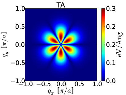
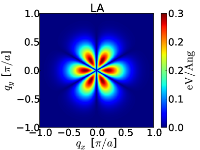
Figure 8: (Color online) Piezoelectric interaction in a 2D hexagonal lattice. The plots show the absolute value of the coupling matrix element $M_{\mathbf{q}\lambda}^{\text{PE}}$ in Eq. 50 for the TA (left) and LA (right) phonon as a function of the phonon wave vector $\mathbf{q}$. The parameters for MoS₂ in Tab. 1 have been used.

The piezoelectric el-ph interaction in Eq. (B) is now given by $H_{\mathbf{q}\lambda}^{\text{PE}}(z)=-e\phi_{\mathbf{q}\lambda}(z)$, and assuming, for simplicity, a Gaussian envelope in Eq. (B), the long-wavelength limit of the piezoelectric coupling matrix element becomes Kaasbjerg et al. (2012a)

$$M_{\mathbf{q}\lambda}^{\text{PE}}=\frac{e_{11}e}{\epsilon_{0}}q\times\text{erfc}(q\sigma/2)A_{\lambda}(\hat{\mathbf{q}}),$$ (50)

where $\sigma$ is the effective width of the electronic envelope function. The piezoelectric interaction has the general property that $M_{-\mathbf{q}\lambda}^{\text{PE}}=-M_{\mathbf{q}\lambda}^{\text{PE}}$ Mahan (2010). The absolute value of the piezoelectric interaction (50) is shown in Fig. 8. Here, the six fold rotational symmetry stems from the hexagonal crystal lattice and is accounted for by the anisotropy factors in Eq. (48).

Contrary to the 3D bulk case where the piezoelectric interaction is independent of $q$ Mahan (2010), the 2D interaction in Eq. (50) depends on the magnitude of the phonon wave vector and acquires a linear $q$-dependence for $q\rightarrow 0$. The latter is a consequence of the 2D crystal lattice which does not support a piezoelectric potential from the acoustic phonons in the long-wavelength limit (see Eq. (B.2)).

Appendix C First-principles calculation of the el-ph interaction

In this appendix, we present the first-principles method applied in the calculation of the el-ph interaction. In order to support the new developments included in this work, we start by briefly highlighting the most important aspects of the main method presented in full detail in Ref. Kaasbjerg et al., 2012a.

The coupling matrix element $M_{\mathbf{k}\mathbf{q}}^{\lambda}$ in the el-ph interaction in Eq. (6) of the main text involves the change in the crystal potential $\delta V_{\mathbf{q}\lambda}$ due to a phonon with wave vector $\mathbf{q}$ and branch index $\lambda$. Under the assumption that the atomic displacements are small, the phonon-induced change in the potential can be constructed as a sum over individual atomic gradients,

$$\delta V_{\mathbf{q}\lambda}(\mathbf{r})=\frac{1}{N}\sum_{\alpha l}e^{i\mathbf{q}\cdot\mathbf{R}_{l}}\hat{\mathbf{e}}_{\mathbf{q}\lambda}^{\alpha}\cdot\nabla_{\alpha l}V(\mathbf{r}).$$ (51)

Here, $\alpha$ is an atomic index in the primitive unit cell, $\mathbf{R}_{l}$ is the lattice vector of unit cell $l$ (relative to the reference unit cell at $\mathbf{R}_{0}$), $\hat{\mathbf{e}}_{\mathbf{q}\lambda}$ is the mass-scaled phonon polarization vector, $\nabla_{\alpha l}$ denotes the gradient with respect to displacements of atom $(\alpha,l)$ in the $x,y,z$ directions, $V$ is the crystal potential, and $N$ is the number of unit cells in the lattice.

The matrix element of the phonon-induced potential between the Bloch states with wave vectors $\mathbf{k}$ and $\mathbf{k}+\mathbf{q}$ are evaluated by expanding the Bloch function in an LCAO basis. The resulting expression for the matrix element follows by exploiting the periodicity of the crystal lattice and takes the form Kaasbjerg et al. (2012a)

$$M_{\mathbf{k}\mathbf{q}}^{\lambda} =\langle\mathbf{k+q}\rvert\delta V_{\mathbf{q}\lambda}(\mathbf{r})\lvert\mathbf{k}\rangle$$

$$=\frac{1}{N}\sum_{ij}c_{i}^{*}c_{j}\sum_{mn}e^{i\mathbf{k}\cdot(\mathbf{R}_{n}-\mathbf{R}_{m})-i\mathbf{q}\cdot\mathbf{R}_{m}}$$

$$\quad\times\langle i\mathbf{R}_{m}\rvert\hat{\mathbf{e}}_{\mathbf{q}\lambda}\cdot\nabla_{0}V(\mathbf{r})\lvert j\mathbf{R}_{n}\rangle,$$ (52)

where $i=(\alpha,\mu)$ is a composite atomic ($\alpha$) and orbital ($\mu$) index, $\lvert i\mathbf{R}_{m}\rangle$ denotes the atomic orbital $\mu$ on atom $\alpha$ in the primitive unit cell $m$, $c_{i}$ are the LCAO expansion coefficients, and $\nabla_{0}V$ is the gradient of the crystal potential with respect to atomic displacements in the reference unit cell. The quantity in the last line of Eq. (C) is the LCAO supercell matrix of the potential gradient. The real-space structure of its matrix elements is illustrated schematically in Fig. 9.

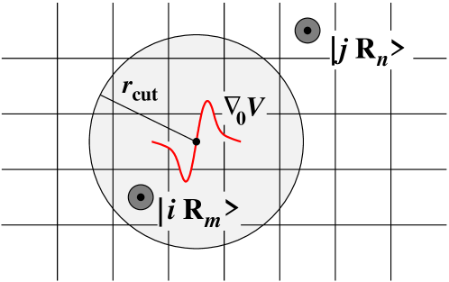
Figure 9: (Color online) Schematic illustration of the LCAO supercell matrix involved in the calculation of the el-ph coupling in Eq. (C). The square lattice indicates the unit cells of the crystal lattice. The real-space cutoff $r_{\text{cut}}$ measured from the position of the atomic site where the gradient of the potential is taken is used to separate out the short- and long-range part of the el-ph interaction. Matrix elements involving LCAO orbitals located beyond the cutoff as the one shown are defined as long range (see also Eq. (53)).

C.1 Real-space separation of the short and long-range part of the electron-phonon interaction

In first-principles calculations of the el-ph interaction both short range (deformation potential) and long range (piezoelectric and Fröhlich interaction) are included in the coupling in Eq. (6). However, due to their different origin it may sometimes be desirable to consider them separately. In the following we outline a real-space partitioning scheme to separate the short-range and long-range contributions to the el-ph interaction.

The central quantity of the partitioning scheme is the LCAO supercell matrix illustrated schematically in Fig. 9. The partitioning scheme consists in splitting up the summations in Eq. (C) into two contributions; (i) a short-range part which neglects all matrix elements involving LCAO orbitals beyond a chosen real-space cutoff $r_{\text{cut}}$, and (ii) a long-range part which includes the remaining matrix elements; i.e.

$$\langle i\mathbf{R}_{m}\rvert\nabla_{\alpha 0}V(\mathbf{r})\lvert j\mathbf{R}_{n}\rangle\rightarrow\left\{\begin{array}[]{l}\text{short-range,}\;\lvert\mathbf{R}_{im}-\mathbf{R}_{k0}\rvert<r_{\text{cut}}\;\text{and}\;\lvert\mathbf{R}_{jn}-\mathbf{R}_{k0}\rvert<r_{\text{cut}}\\ \\ \text{long-range,}\;\lvert\mathbf{R}_{im/jn}-\mathbf{R}_{k0}\rvert>r_{\text{cut}}\end{array}\right.$$ (53)

where $\mathbf{R}_{mi}=\mathbf{R}_{m}+\mathbf{R}_{\alpha}$ denotes the atomic positions of the LCAO orbitals and the potential gradients.

In general, the real-space cutoff $r_{\text{cut}}$ must be chosen small enough that the short-range part does not include contributions from truly long-range effects in the relevant range of phonon wave vectors; i.e. $\pi/r_{\text{cut}}>q_{\text{max}}$ where $q_{\text{max}}$ is the maximum phonon wave vector of interest. At the same time, the cutoff cannot be chosen too small that short-range effects are cut off. As these guidelines do not provide a unique way to choose the real-space cutoff, it should be verified in an actual calculation that the results do not change significantly for different values of the cutoff.

Deformation potential interaction

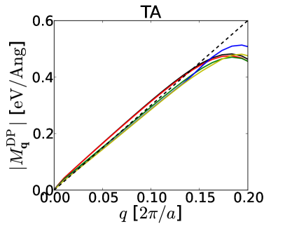
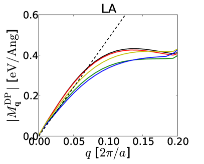
Piezoelectric interaction

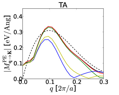
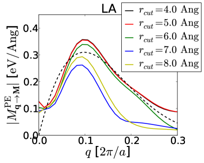
Figure 10: (Color online) Deformation potential (upper row) and piezoelectric (lower row) interactions in monolayer MoS₂ obtained with the real-space partitioning scheme for different values of the real-space cutoff $r_{\text{cut}}$. The plots show the absolute value of the matrix elements $M_{\mathbf{q}\lambda}^{\text{DP/PE}}$ averaged over the high-symmetry directions of the hexagonal lattice. The analytic couplings in Eqs. (11) and (13) are shown with dashed lines for the MoS₂ parameters listed in Tab. 1.

In Fig. 10 we show the deformation potential (top row) and piezoelectric (bottom row) interactions for the TA and LA phonons in 2D MoS₂ obtained with the partitioning scheme for different values of the cutoff foo (b). The dashed lines show the analytic forms for the deformation potential and piezoelectric interactions in Eqs. (11) and (13) with the parameters listed in Tab. 1. While the variation in the deformation potential interaction is relatively insignificant, the piezoelectric interaction is more sensitive to the chosen cutoff. The best agreement between the analytic expression for the piezoelectric interaction in Eq. (13) and the first-principles results is obtained for $r_{\text{cut}}=6.0$ Å.

It should be emphasized that the finite value of the first-principles piezoelectric interaction in the limit $q\rightarrow 0$ in Fig. 10 is an artifact inherent to a supercell method. The finite real-space range of the el-ph interaction in supercell methods naturally sets a lower limit for the magnitude of the phonon wave vector $q_{\text{min}}$ at which long-range interactions can be obtained reliably. It is given by $q_{\text{min}}=2\pi/L_{\text{cell}}$ where $L_{\text{cell}}$ is the size of the supercell (measured as the diameter of a sphere that can be contained within the supercell). In the calculations presented here $L_{\text{cell}}\sim 45$ Å implying that $q_{\text{min}}\sim 0.14$ Å${}^{-1}\sim 0.07\times 2\pi/a$.

The real-space partitioning scheme outlined here can also be applied in other first-principles calculations of the el-ph interaction based on e.g. Wannier functions Giustino et al. (2007).

C.2 Normal and umklapp processes

In order identify the normal and umklapp processes in the el-ph interaction, we start by noticing that the gradients of the potential $\nabla_{\alpha l}V\equiv\mathbf{f}_{\alpha}(\mathbf{r}-\mathbf{R}_{l})$ in Eq. (51) are localized functions in real space (see Fig. 9), where $\mathbf{f}_{\alpha}$ denotes an atom-specific function. Due to the periodicity of the lattice, the gradient in unit cell $l$ is related to the gradient in the reference cell through a translation by the lattice vector $\mathbf{R}_{l}$. We now express the gradients of the potential in terms of their Fourier series,

$$\nabla_{\alpha l}V(\mathbf{r})=\sum_{\bm{\kappa}}e^{i\bm{\kappa}\cdot(\mathbf{r}-\mathbf{R}_{l})}\mathbf{f}_{\bm{\kappa}}^{\alpha},$$ (54)

where $\bm{\kappa}=(\bm{\kappa}_{\parallel},\bm{\kappa}_{\perp})$ is a three-dimensional Fourier variable. It is here important to distinguish between the projections $\bm{\kappa}_{\parallel}/\bm{\kappa}_{\perp}$ of $\bm{\kappa}$ onto the periodic/nonperiodic directions of the lattice. The sum over the unit cell index $l$ in Eq. (51) now only contains two exponential factors,

$$\sum_{l}e^{i(\mathbf{q}-\bm{\kappa}_{\parallel})\cdot\mathbf{R}_{l}}=N\delta_{\bm{\kappa}_{\parallel},\mathbf{q}+\mathbf{G}},$$ (55)

where the reciprocal lattice vector $\mathbf{G}$ and the phonon wave vector $\mathbf{q}$ by definition have the dimensionality of the lattice. This restricts the projection $\bm{\kappa}_{\parallel}$ to values $\mathbf{q}+\mathbf{G}$. Inserting in Eq. (51), we find for the phonon-induced potential

$$\delta V_{\mathbf{q}\lambda}(\mathbf{r}) =\sum_{\mathbf{G}}e^{i(\mathbf{q}+\mathbf{G})\cdot\mathbf{r}_{\parallel}}\sum_{\bm{\kappa}_{\perp}\alpha}e^{i\bm{\kappa}_{\perp}\cdot\mathbf{r}_{\perp}}\hat{\mathbf{e}}_{\mathbf{q}\lambda}^{\alpha}\cdot\mathbf{f}_{(\mathbf{q}+\mathbf{G},\bm{\kappa}_{\perp})}^{\alpha}$$

$$\equiv\sum_{\mathbf{G}}e^{i(\mathbf{q}+\mathbf{G})\cdot\mathbf{r}_{\parallel}}\delta V_{\mathbf{q}+\mathbf{G}}^{\lambda}(\mathbf{r}_{\perp}).$$ (56)

First of all, we note that this allows us write the phonon-induced potential on the Bloch form in Eq. (9). Secondly, the separation into normal ($\mathbf{G}=\mathbf{0}$) and umklapp ($\mathbf{G}\neq\mathbf{0}$) processes is now formally straight-forward.

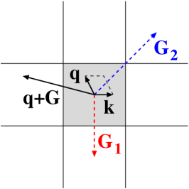
Figure 11: (Color online) Schematic illustration of an umklapp process involving a Fourier component of the scattering potential at $\mathbf{q}+\mathbf{G}$. The square lattice denotes the reciprocal lattice with the shaded cell indicating the first Brillouin zone. The dashed arrows show a pair of reciprocal lattice vectors $\mathbf{G}_{1/2}$ from the electronic Bloch functions that conserve crystal momentum by bringing $\mathbf{q}+\mathbf{G}$ back onto $\mathbf{q}$ in the first Brillouin zone.

It is important to note that in first-principles calculations of the el-ph interaction, the term “umklapp process” has a more general meaning than the one encountered in conventional textbook discussions of the subject Madelung (1996). In order to illustrate this, it is instructive to evaluate the matrix element $M_{\mathbf{k}\mathbf{q}}^{\lambda}$ in Eq. (C) with the electronic Bloch functions expanded as $\psi_{\mathbf{k}}(\mathbf{r})=\sum_{\mathbf{G}}e^{i(\mathbf{k}+\mathbf{G})\cdot\mathbf{r}_{\parallel}}u_{\mathbf{k}+\mathbf{G}}(\mathbf{r}_{\perp})$, where $u_{\mathbf{k}+\mathbf{G}}$ are the Fourier components of the periodic part of the Bloch functions. This yields

$$M_{\mathbf{k}\mathbf{q}}^{\lambda} =\langle\mathbf{k+q}\rvert\delta V_{\mathbf{q}\lambda}(\mathbf{r})\lvert\mathbf{k}\rangle$$

$$=\sum_{\mathbf{G}}\sum_{\mathbf{G}_{1}\mathbf{G}_{2}}u_{\mathbf{k}+\mathbf{q}+\mathbf{G}_{1}}^{*}\delta V_{\mathbf{q}+\mathbf{G}}^{\lambda}u_{\mathbf{k}+\mathbf{G}_{2}}$$

$$\quad\times\underbrace{\int\!d\mathbf{r}_{\parallel}\,e^{i(\mathbf{G}+\mathbf{G}_{1}+\mathbf{G}_{2}-\mathbf{G}_{3})\cdot\mathbf{r}_{\parallel}}}_{=\delta_{\mathbf{G}_{3},\mathbf{G}+\mathbf{G}_{1}+\mathbf{G}_{2}}},$$ (57)

where $\mathbf{G}_{1/2}$ are the reciprocal lattice vectors from the Bloch functions, $\mathbf{G}_{3}$ is a reciprocal lattice vector that shifts $\mathbf{k}+\mathbf{q}$ to the first Brillouin zone in case it falls outside, and the $\mathbf{r}_{\perp}$ dependence has been integrated out. The $\delta$ function resulting from the integral in the last line can be regarded as a generalized statement of conservation of crystal momentum taking into account the reciprocal lattice vectors from the Bloch functions. It differs from the standard textbook definition where $\mathbf{G}_{1/2}=\mathbf{0}$ and $\mathbf{G}=\mathbf{G}_{3}$ implying that umklapp processes only contribute to the matrix element if $\mathbf{G}_{3}\neq\mathbf{0}$; i.e. $\mathbf{k}+\mathbf{q}\notin\text{1. BZ}$ Madelung (1996). For the generalized conservation of crystal momentum this is not the case. Here, umklapp processes involving all Fourier components $\mathbf{G}$ of the scattering potential contribute regardless of the value of $\mathbf{G}_{3}$. This is illustrated in Fig. 11 which shows an umklapp process ($\mathbf{G}\neq\mathbf{0}$) for $\mathbf{G}_{3}=\mathbf{0}$ and a $(\mathbf{G}_{1},\mathbf{G}_{2})$ pair that conserves crystal momentum. For intravalley scattering where $\mathbf{k}+\mathbf{q}$ is always inside the first Brillouin zone (if not, the first Brillouin zone can chosen such that this is the case) and hence $\mathbf{G}_{3}=\mathbf{0}$, coupling to phonons via umklapp processes takes place through the type of process shown in Fig. 11.

In the following section we outline a Fourier filtering method which allows for a numerical separation of normal and umklapp processes in the supercell method.

C.2.1 Fourier filtering method

In practice, the matrix elements of the el-ph interaction are evaluated using Eq. (C). The expression for the phonon-induced potential change in Eq. (C.2) is therefore not directly applicable for the separation of the normal and umklapp processes. Instead we note that the sum over unit cell indices $l$ in Eq. (55) provides an automatic selection of the Fourier components in $\nabla_{0}V$ that contribute in Eq. (C.2). The Fourier expansion of $\nabla_{0}V$ can therefore be used directly in the calculation of the matrix element in Eq. (C). Writing the Fourier expansion as

$$\nabla_{0}V(\mathbf{r}) =\sum_{\bm{\kappa_{\parallel}}\in 1.\text{BZ}}e^{i\bm{\kappa_{\parallel}}\cdot\mathbf{r}_{\parallel}}\mathbf{f}_{\bm{\kappa}_{\parallel}}(\mathbf{r}_{\perp})$$

$$\quad+\sum_{\bm{\kappa_{\parallel}}\notin 1.\text{BZ}}e^{i\bm{\kappa_{\parallel}}\cdot\mathbf{r}_{\parallel}}\mathbf{f}_{\bm{\kappa}_{\parallel}}(\mathbf{r}_{\perp}),$$ (58)

the two terms with $\bm{\kappa}_{\parallel}$ lying inside and outside the Brillouin zone (BZ) of the crystal lattice define the normal and umklapp contribution to the el-ph interaction, respectively.

Numerically, the atomic gradients $\nabla_{0}V$ are represented on a three-dimensional real-space grid in the supercell having length $L_{i}$ and $N_{i}$ number of grid points in the direction of the lattice vector $\mathbf{a}_{i}$. The resulting grid spacing is $\Delta x_{i}=L_{i}/N_{i}$. The values of the gradients on the grid are denoted $\mathbf{f}_{ijk}$. The Fourier expansion is obtained using the fast Fourier transform (FFT),

$$\mathbf{f}_{\kappa_{i}\kappa_{j}\kappa_{k}}=\text{FFT}(\mathbf{f}_{ijk}),$$ (59)

with the corresponding Fourier space grid in the direction of the primitive reciprocal lattice vector $\mathbf{b}_{i}$ given by $\kappa_{i}=-\kappa_{i,\text{max}}+n\Delta\kappa_{i}$ with $n=0,1,2,\ldots,N_{i}-1$, $\Delta\kappa_{i}=2\pi/L_{i}$ and $\kappa_{i,\text{max}}=\pi/\Delta x_{i}$. As the supercell has a real-space grid spacing significantly smaller and a size significantly larger than the lattice constant $a$, i.e. $\Delta x_{i}\ll a$ and $L_{i}\gg a$, respectively, we have that $\kappa_{i,\text{max}}\gg\pi/a$ and $\Delta\kappa_{i}\ll\pi/a$.

The normal and umklapp processes can now be separated by Fourier filtering $\mathbf{f}_{\kappa_{i}\kappa_{j}\kappa_{k}}$. This is done by zeroing the Fourier components at $\bm{\kappa}=(\kappa_{i},\kappa_{j},\kappa_{k})$ with $\bm{\kappa}_{\parallel}$ lying outside or inside the Brillouin zone. Using a tilde to denote the filtered quantities, we have

$$\mathbf{\tilde{f}}_{\kappa_{i}\kappa_{j}\kappa_{k}}\rightarrow\left\{\begin{array}[]{l}\text{normal,}\;\neq 0\;\text{if}\;\bm{\kappa_{\parallel}}\in 1.\text{BZ}\\ \text{umklapp,}\;\neq 0\;\text{if}\;\bm{\kappa_{\parallel}}\notin 1.\text{BZ}\end{array}\right..$$ (60)

Applying the inverse FFT (IFFT)

$$\mathbf{\tilde{f}}_{ijk}=\text{IFFT}(\mathbf{\tilde{f}}_{\kappa_{i}\kappa_{j}\kappa_{k}}),$$ (61)

we obtain the filtered gradients in real space which can be used in the numerical evaluation of the matrix element in Eq. (C). Since the gradients of the potential $\nabla_{0}V$ are real valued, the imaginary part of $\mathbf{\tilde{f}}_{ijk}$ can be discarded.

References

- Novoselov et al. (2005) K. S. Novoselov, D. Jiang, F. Schedin, T. J. Booth, V. V. Khotkevich, S. V. Morozov, and A. K. Geim, PNAS 102, 10451 (2005).
- Geim and Novoselov (2007) A. K. Geim and K. S. Novoselov, Nature Mat. 6, 183 (2007).
- Neto et al. (2009) A. H. C. Neto, F. Guinea, N. M. R. Peres, K. S. Novoselov, and A. K. Geim, Rev. Mod. Phys. 81, 109 (2009).
- Das Sarma et al. (2011) S. Das Sarma, S. Adam, E. H. Hwang, and E. Rossi, Rev. Mod. Phys. 83, 407 (2011).
- Wang et al. (2012) Q. H. Wang, K. Kalantar-Zadeh, A. Kis, J. N. Coleman, and M. S. Strano, Nature Nano. 7, 699 (2012).
- Chhowalla et al. (2013) M. Chhowalla, H. S. Shin, G. Eda, L.-J. Li, K. P. Loh, and H. Zhang, Nature Chem. 5, 263 (2013).
- Podzorov et al. (2004) V. Podzorov, M. E. Gershenson, C. Kloc, R. Zeis, and E. Bucher, Appl. Phys. Lett. 84, 3301 (2004).
- Mak et al. (2010) K. F. Mak, C. Lee, J. Hone, J. Shan, and T. F. Heinz, Phys. Rev. Lett. 105, 136805 (2010).
- Splendiani et al. (2010) A. Splendiani, L. Sun, Y. Zhang, T. Li, J. Kim, C.-Y. Chim, G. Galli, and F. Wang, Nano. Lett. 10, 1271 (2010).
- Radisavljevic et al. (2011) B. Radisavljevic, A. Radenovic, J. Brivio, V. Giacometti, and A. Kis, Nature Nano. 6, 147 (2011).
- Korn et al. (2011) T. Korn, S. Heydrich, M. Hirmer, J. Schmutzler, and C. Schüller, Appl. Phys. Lett. 99, 102109 (2011).
- Zhang et al. (2012) Y. Zhang, J. Ye, Y. Matsuhashi, and Y. Iwasa, Nano. Lett. 12, 1136 (2012).
- Xiao et al. (2012) D. Xiao, G.-B. Liu, W. Feng, X. Xu, and W. Yao, Phys. Rev. Lett. 108, 196802 (2012).
- Cao et al. (2012) T. Cao, G. Wang, W. Han, H. Ye, C. Zhu, J. Shi, Q. Niu, P. Tan, E. Wang, B. Liu, et al., Nature Commun. 3, 887 (2012).
- Mak et al. (2012) K. F. Mak, K. He, J. Shan, and T. F. Heinz, Nature Nano. 7, 494 (2012).
- Zeng et al. (2012) H. Zeng, J. Dai, W. Yao, D. Xiao, and X. Cui, Nature Nano. 7, 490 (2012).
- Ayari et al. (2007) A. Ayari, E. Cobas, O. Ogundadegbe, and M. S. Fuhrer, J. Appl. Phys. 101, 014507 (2007).
- Matte et al. (2010) H. S. S. R. Matte, A. Gomathi, A. K. Manna, D. J. Late, R. Datta, S. K. Pati, and C. N. R. Rao, Angew. Chem. 122, 4153 (2010).
- Liu et al. (2012) K.-K. Liu, W. Zhang, Y.-H. Lee, Y.-C. Lin, M.-T. Chang, C.-Y. Su, C.-S. Chang, H. Li, Y. Shi, H. Zhang, et al., Nano. Lett. 12, 1538 (2012).
- Liu and Ye (2012) H. Liu and P. D. Ye, IEEE Electron Devices Letters 33, 546 (2012).
- Kim et al. (2012) S. Kim, A. Konar, W. Hwang, J. H. Lee, J. Lee, J. Yang, C. Jung, H. Kim, J. Yoo, J. Choi, et al., Nature Commun. 3, 1011 (2012).
- Fallahazad and Tutuc (2012) S. L. B. Fallahazad and E. Tutuc, Appl. Phys. Lett. 101, 223104 (2012).
- Fuhrer and Hone (2013) M. S. Fuhrer and J. Hone, Nature Nano. 8, 146 (2013).
- Radisavljevic and Kis (2013) B. Radisavljevic and A. Kis, Nature Nano. 8, 147 (2013).
- Jena and Konar (2007) D. Jena and A. Konar, Phys. Rev. Lett. 98, 136805 (2007).
- Kaasbjerg et al. (2012a) K. Kaasbjerg, K. S. Thygesen, and K. W. Jacobsen, Phys. Rev. B 85, 115317 (2012a).
- Yoon et al. (2011) Y. Yoon, K. Ganapathi, and S. Salahuddin, Nano. Lett. 11, 3768 (2011).
- Popov et al. (2012) I. Popov, G. Seifert, and D. Tománek, Phys. Rev. Lett. 108, 156802 (2012).
- Hwang and Das Sarma (2008a) E. H. Hwang and S. Das Sarma, Phys. Rev. B 77, 235437 (2008a).
- Price (1984) P. J. Price, Solid State Commun. 51, 607 (1984).
- Stormer et al. (1990) H. L. Stormer, L. N. Pfeiffer, K. W. Baldwin, and K. W. West, Phys. Rev. B 41, 1278 (1990).
- Efetov and Kim (2010) D. K. Efetov and P. Kim, Phys. Rev. Lett. 105, 256805 (2010).
- Hwang and Das Sarma (2008b) E. H. Hwang and S. Das Sarma, Phys. Rev. B 77, 115449 (2008b).
- Castro et al. (2010) E. V. Castro, H. Ochoa, M. I. Katsnelson, R. V. Gorbachev, D. C. Elias, K. S. Novoselov, A. K. Geim, and F. Guinea, Phys. Rev. Lett. 105, 266601 (2010).
- Kaasbjerg et al. (2012b) K. Kaasbjerg, K. S. Thygesen, and K. W. Jacobsen, Phys. Rev. B 85, 165440 (2012b).
-
foo (a)
The chemical potential of a 2DEG is related to the carrier
density via
where is the effective density of states at the band edge. For the valley-degenerate () conduction band of MoS2, the effective density of states is cm-2 with measured in K. In the degenerate high-density limit , the Fermi level becomes () with measured in units of cm-2. - Das et al. (2008) A. Das, S. Pisana, B. Chakraborty, S. Piscanec, S. K. Saha, U. V. Waghmare, K. S. Novoselov, H. R. Krishnamurthy, A. K. Geim, A. C. Ferrari, et al., Nature Nano. 3, 210 (2008).
- Chakraborty et al. (2012) B. Chakraborty, A. Bera, D. V. S. Muthu, S. Bhowmick, U. V. Waghmare, and A. K. Sood, Phys. Rev. B 85, 161403 (2012).
- Kawamura and Das Sarma (1990) T. Kawamura and S. Das Sarma, Phys. Rev. B 42, 3725 (1990).
- Knäbchen (1997) A. Knäbchen, Phys. Rev. B 55, 6701 (1997).
- Mori and Ando (1989) N. Mori and T. Ando, Phys. Rev. B 40, 6175 (1989).
- Chen et al. (2008) J.-H. Chen, C. Jang, S. Xiao, M. Ishigami, and M. S. Fuhrer, Nature Nano. 3, 206 (2008).
- Fratini and Guinea (2008) S. Fratini and F. Guinea, Phys. Rev. B 77, 195415 (2008).
- Konar et al. (2010) A. Konar, T. Fang, and D. Jena, Phys. Rev. B 82, 115452 (2010).
- Zhang et al. (2013) S. H. Zhang, W. Xu, S. M. Badalyan, and F. M. Peeters, Phys. Rev. B 87, 075443 (2013).
- Min et al. (2012) H. Min, E. H. Hwang, and S. Das Sarma, Phys. Rev. B 86, 085307 (2012).
- Lebègue and Eriksson (2009) S. Lebègue and O. Eriksson, Phys. Rev. B 79, 115409 (2009).
- Cheiwchanchamnangij and Lambrecht (2012) T. Cheiwchanchamnangij and W. R. L. Lambrecht, Phys. Rev. B 85, 205302 (2012).
- Zhu et al. (2011) Z. Y. Zhu, Y. C. Cheng, and U. Schwingenschlögl, Phys. Rev. B 84, 153402 (2011).
- Chen et al. (2007) L. Chen, Z. Ma, J. C. Cao, T. Y. Zhang, and C. Zhang, Appl. Phys. Lett. 91, 102115 (2007).
- Biswas and Ghosh (2013) T. Biswas and T. K. Ghosh, J. Phys.: Condens. Matter 25, 035301 (2013).
- Kawamura and Das Sarma (1992) T. Kawamura and S. Das Sarma, Phys. Rev. B 45, 3612 (1992).
- Mortensen et al. (2005) J. J. Mortensen, L. B. Hansen, and K. W. Jacobsen, Phys. Rev. B 71, 035109 (2005).
- Larsen et al. (2009) A. H. Larsen, M. Vanin, J. J. Mortensen, K. S. Thygesen, and K. W. Jacobsen, Phys. Rev. B 80, 195112 (2009).
- Enkovaara et al. (2010) J. . Enkovaara, C. Rostgaard, J. J. Mortensen, J. Chen, M. Dulak, L. Ferrighi, J. Gavnholt, C. Glinsvad, V. Haikola, H. A. Hansen, et al., J. Phys.: Condens. Matter 22, 253202 (2010).
- Mahan (2010) G. D. Mahan, Many-particle Physics (Springer, 2010), 3rd ed.
- foo (b) The electron-phonon coupling has been calculated with DFT-LDA using a supercell, a double-zeta polarized (DZP) basis for the electronic Bloch states, and 5 Å of vacuum between the MoS2 sheet and the cell boundaries in the direction perpendicular to the sheet. In this direction non-periodic boundary conditions must be applied in order to avoid spurious interlayer contributions to the long-range part of the electron-phonon interaction in the long-wavelength limit (which are present when periodic boundary conditions are applied). A real-space cutoff of Å has been used to separate out the short-range deformation potential and long-range piezoelectric interactions.
- Madelung (1996) O. Madelung, Introduction to Solid State Physics (Springer, Berlin, 1996).
- Sai and Mele (2003) N. Sai and E. J. Mele, Phys. Rev. B 68, 241405 (2003).
- foo (c) Due to a different choice of the primitive lattice vectors in App. B.2 and our first-principles calculations (see Fig. 1), the angular dependencies of the matrix elements for the TA and LA phonons in Eq. (14) are interchanged compared to the ones in Fig. 2.
- Duerloo et al. (2012) K.-A. N. Duerloo, M. T. Ong, and E. J. Reed, J. Phys. Chem. Lett. 3, 2871 (2012).
- foo (d) Ideally, this only holds for oriented along high-symmetry directions of the hexagonal lattice where is an even function of such that the angular integration of the factor in Eq. (4) vanishes.
- Hybertsen and Louie (1987) M. S. Hybertsen and S. G. Louie, Phys. Rev. B 35, 5585 (1987).
- Ando et al. (1982) T. Ando, A. B. Fowler, and F. Stern, Rev. Mod. Phys. 54, 437 (1982).
- Maldague (1978) P. F. Maldague, Surf. Sci. 73, 296 (1978).
- Flensberg and Hu (1995) K. Flensberg and B. Y. Hu, Phys. Rev. B 52, 14796 (1995).
- Yan et al. (2011) J. Yan, J. J. Mortensen, K. W. Jacobsen, and K. S. Thygesen, Phys. Rev. B 83, 245122 (2011).
- Walukiewicz et al. (1984) W. Walukiewicz, H. E. Ruda, J. Lagowski, and H. C. Gatos, Phys. Rev. B 30, 4571 (1984).
- foo (e) The field is here applied in the direction of the in-plane projection of the Mo-S bonds.
- Song and Dery (2013) Y. Song and H. Dery (2013), arXiv:1302.3627.
- Giustino et al. (2007) F. Giustino, M. L. Cohen, and S. G. Louie, Phys. Rev. B 76, 165108 (2007).