Nonequilibrium Green’s function theory of coherent excitonic effects in the photocurrent response of semiconductor nanostructures

Abstract

Excitonic contributions to absorption and photocurrent generation in semiconductor nanostructures are described theoretically and simulated numerically using steady-state non-equilibrium Green’s function theory. In a first approach, the coherent interband polarization including Coulomb corrections is determined from a Bethe-Salpeter-type equation for the equal time interband single-particle charge carrier Green’s function. The effects of excitonic absorption on photocurrent generation are considered on the same level of approximation via the derivation of the corresponding corrections to the electron-photon self-energy.

I Introduction

Recently, the investigation of semiconductor nanostructures for photovoltaic applications has been of ever growing interest. Potential candidates among these low dimensional absorbers are ordered configurations of quantum wells (QW) Ekins-Daukes et al. (1999); Green (2000) or quantum dots (QD) Conibeer et al. (2006); Martí et al. (2006), which are widely used in other optoelectronic devices such as lasers or light-emitting devices. However, due to the unique operating regime of solar cells, optical and transport properties are equally important, and should not be considered in the isolated nanostructure component, but for an open system connected to the environment via contacts. Since the main attraction of the systems is the presence of quantum confinement effects that can be exploited to enhance the photovoltaic performance, a comprehensive description should be on the level of a quantum transport theory. Such a theory was recently developed on the example of QW solar cells Aeberhard and Morf (2008); Aeberhard (2011, 2011) and applied to QD solar cells Aeberhard (2012).

Excitonic effects play only a minor role in conventional inorganic bulk semiconductor solar cells, since in most cases, the exciton binding energies are small as compared to the thermal broadening at room temperature, and exciton dissociation is very fast as nothing hinders the spatial separation of the carriers. However, this is not the case in quantum confined systems, where the strong localization of the electron and hole wave functions leads to a large overlap and thus substantially larger exciton binding energies. As a consequence, the excitonic features in the optoelectronic properties persist up to room temperature and have therefore considerable impact on the photovoltaic properties of devices based on such systems. In the past, excitonic effects in semiconductor nanostructures have been discussed for steady state linear absorption or in the regime of high-intensity pulse excitation. For the latter, sophisticated quantum-kinetic theories were developed Haug and Schmitt-Rink (1984); Haug and Henneberger (1988); Haug (1992); Haug and Jauho (1996); Haug and Koch (2004); Henneberger and May (1986); Henneberger (1988, 1988); Henneberger and Haug (1988); Henneberger and Koch (1996); Jahnke and Koch (1995). For the description of quantum photovoltaic devices, the picture of coherent excitonic absorption needs to be combined with a steady state quantum transport formalism. A suitable theoretical framework is provided by the non-equilibrium Green’s function formalism. However, the shifting of the focus from transient interband kinetics to steady-state transport does not allow for a straight-forward inclusion of excitonic processes: while in the former case coherent excitonic polarization can be included via the Fock term of Coulomb interaction to lowest order, there is no equal-time approximation in the latter situation. This paper thus aims at the inclusion of excitonic effects into a general theory of quantum opto-electronics including the transport aspect, which should allow for the study of photovoltaic systems where these effects dominate the photocurrent response close to the absorption edge.

The paper is organized as follows. In the section after this introduction, the coupling of charge carriers to the coherent radiation fields is described based on the NEGF theory for a two-band model of a direct gap semiconductor, followed by a derivation of the coherent interband polarization and the effective interband self-energy due to Coulomb-enhanced electron-photon interaction. In a further section, these results are used in the simulation of the photocurrent respose of bulk and thin film devices, where the latter case is represented by a single quantum well III-V semiconductor $p$-$i$-$n$ diode.

II NEGF model of a contacted excitonic absorber

II.1 Hamiltonian, Green’s functions and self energies

As a suitable model system, we choose a simple two band model of a direct gap semiconductor nanostructure selectively connected to ohmic contacts Aeberhard and Morf (2008) and coupled to a coherent external photon field, which at this stage is treated classically. Since we are interested in the photocurrent response of the system, only the electronic part of the system is considered via the Hamiltonian

$$\hat{H}=\hat{H}_{0}+\hat{H}_{e\gamma}+\hat{H}_{ep}+\hat{H}_{ee}+\hat{H}_{C}.$$ (1)

$\hat{H}_{0}$ is the Hamiltonian of the non-interacting isolated mesoscopic absorber, $\hat{H}_{e\gamma}$ is the light-matter coupling, $\hat{H}_{ep}$ encodes the electron-phonon and $\hat{H}_{ee}$ the carrier-carrier interaction. The last term $\hat{H}_{C}$ describes the (selective) coupling to contacts required for carrier extraction in order to enable photocurrent flow. The charge carriers in the two bands $b=c,v$ are described by the field operators $\hat{\Psi}_{b}(\mathbf{r},t)$, which provides the Hamiltonian representation

$$\mathcal{H}(t)=\sum_{a,b=c,v}\int d^{3}r\hat{\Psi}_{a}^{\dagger}(\mathbf{r},t)\hat{H}(\mathbf{r},t)\hat{\Psi}_{b}(\mathbf{r},t).$$ (2)

The renormalizing effects of the interaction and contact Hamiltonian terms on the isolated system are expressed within non-equilibrium many-body perturbation theory Kadanoff and Baym (1962); Keldysh (1965) in terms of corresponding self-energies entering the generalized Kadanoff-Baym equations for the charge carrier non-equilibrium Green’s functions ($\underline{1}\equiv\{\mathbf{r}_{1},t_{1}\in\mathcal{C}\},\mathcal{C}$: Keldysh contour in the complex plane, $\int{\mathrm{d}}\underline{1}\equiv\int d^{3}r_{1}\int_{\mathcal{C}}dt_{1}$)

$$\mathbf{G}_{0}^{-1}(\underline{1},\underline{1})\mathbf{G}(\underline{1},\underline{1^{\prime}})= \boldsymbol{\delta}(\underline{1},\underline{1^{\prime}})$$

$$+\int{\mathrm{d}}\underline{2}\,\boldsymbol{\Sigma}(\underline{1},\underline{2})\mathbf{G}(\underline{2},\underline{1^{\prime}}),$$ (3)

$$[\mathbf{G}_{0}^{\dagger}]^{-1}(\underline{1^{\prime}},\underline{1^{\prime}})\mathbf{G}(\underline{1},\underline{1^{\prime}})= \boldsymbol{\delta}(\underline{1},\underline{1^{\prime}})$$

$$+\int{\mathrm{d}}\underline{2}\,\mathbf{G}(\underline{1},\underline{2})\boldsymbol{\Sigma}(\underline{2},\underline{1^{\prime}}),$$ (4)

where

$$[G_{0}^{-1}(\underline{1},\underline{1^{\prime}})]_{ab}=\left(i\hbar\frac{\partial}{\partial t_{1}}-[H_{0}(\mathbf{r}_{1})]_{a}\right)\delta(\underline{1},\underline{1^{\prime}})\delta_{ab}$$ (5)

and the contour-ordered Green’s functions are defined via

$$G_{ab}(\underline{1},\underline{1^{\prime}})\equiv-\frac{i}{\hbar}\langle\hat{\Psi}_{a}(\underline{1})\hat{\Psi}_{b}^{\dagger}(\underline{1}^{\prime})\rangle_{\mathcal{C}}$$ (6)

for band indices $a,b$. The self-energy term in the above equations for the Green’s functions may be divided into the contributions from the interactions and the contact term,

$$\boldsymbol{\Sigma}(\underline{1},\underline{2})=\boldsymbol{\Sigma}^{I}(\underline{1},\underline{2})+\boldsymbol{\Sigma}^{C}(\underline{1},\underline{2}),$$ (7)

where the interaction term contains the effects of electron-photon, electron-phonon and electron-electron coupling,

$$\boldsymbol{\Sigma}^{I}(\underline{1},\underline{2})=\boldsymbol{\Sigma}^{e\gamma}(\underline{1},\underline{2})+\boldsymbol{\Sigma}^{ep}(\underline{1},\underline{2})+\boldsymbol{\Sigma}^{ee}(\underline{1},\underline{2}).$$ (8)

Following the standard real-time decomposition rules Langreth (1976) applied to (3) and a special band decoupling procedure described in App. A, the equations for the retarded, advanced, lesser and greater components of the non-equilibrium Green’s functions for charge carriers can be written in the standard intraband form used in transport calculations, ($1\equiv\{\mathbf{r}_{1},t_{1}\in\mathbbm{R}\},~{}\int{\mathrm{d}}1\equiv\int d^{3}r_{1}\int_{-\infty}^{\infty}dt_{1}$)

$$\int{\mathrm{d}}2\,\left[G^{-1}_{0,aa}(1,2)-\tilde{\Sigma}_{aa}^{R}(1,2)\right]G_{aa}^{R}(2,1^{\prime})=\delta(1,1^{\prime}),$$

$$G_{aa}^{<}(1,1^{\prime})=\int{\mathrm{d}}2\int{\mathrm{d}}3\,G_{aa}^{R}(1,2)\tilde{\Sigma}_{aa}^{<}(2,3)G_{aa}^{A}(3,1^{\prime}),$$

$$\qquad\qquad\qquad a\in\{c,v\}$$ (9)

where

$$\tilde{\Sigma}_{aa}^{i}(1,1^{\prime})= \Sigma_{aa}^{i}(1,1^{\prime})+\Sigma_{aa}^{\delta i}(1,1^{\prime}),$$

$$i=R,A,\lessgtr,\quad a\in\{c,v\},$$ (10)

with the effective band-coupling self-energy from the singular contributions given by

$$\Sigma_{aa}^{\delta i}(1,1^{\prime})= \int{\mathrm{d}}2\int{\mathrm{d}}3\,\Sigma_{ab}^{\delta}(1,2)\tilde{G}_{bb}^{i}(2,3)\Sigma_{ba}^{\delta}(3,1^{\prime}),$$

$$i=R,A,\lessgtr,\quad a\neq b,\quad a,b\in\{c,v\}.$$ (11)

In the situation under investigation, the singular interband self-energy itself is of the form

$$\Sigma_{ab}^{\delta}(1,2)= \left[\Sigma_{ab}^{\delta,e\gamma}(\mathbf{r}_{1},t_{1})\delta(\mathbf{r}_{1}-\mathbf{r}_{2})+\Sigma_{ab}^{\delta,ee}(\mathbf{r}_{1},\mathbf{r}_{2},t_{1})\right]$$

$$\times\delta(t_{1}-t_{2}),$$ (12)

where $\Sigma_{ab}^{\delta,e\gamma}$ encodes the coupling of electrons to a coherent photon field and $\Sigma_{ab}^{\delta,ee}$ is the (non-retarded) Fock term of the (screened) Hartree-Fock approximation to carrier-carrier interaction leading to Coulomb enhancement of the optical interband transitions due to the electron-hole coupling.

II.2 Singular self-energy and coherent interband polarization

The self-energy due to the light-matter interaction can be written in terms of the vector potential of the classical electromagnetic field,

$$\Sigma_{ab}^{\delta,e\gamma}(\mathbf{r},t) =-\frac{e}{m_{0}}\langle\hat{\mathbf{A}}(\mathbf{r},t)\rangle\cdot\hat{\mathbf{p}}(\mathbf{r}),$$ (13)

with $\langle\hat{\mathbf{A}}(\mathbf{r},t)\rangle=\mathbf{A}_{coh}(\mathbf{r},t)$. The Coulomb term is

$$\Sigma_{ab}^{\delta,ee}(\mathbf{r}_{1},\mathbf{r}_{2},t)=i\hbar V(\mathbf{r}_{1}-\mathbf{r}_{2})G_{ab}^{<}(\mathbf{r}_{1},\mathbf{r}_{2},t,t^{+}),$$ (14)

where $V$ is the (screened) Coulomb potential, and depends thus on the coherent interband polarization through the interband Green’s function, which the decoupling provides in the form

$$G_{vc}^{<}(1,1^{\prime})= \int d2\int d3\,\Big{[}\tilde{G}_{vv}^{R}(1,2)\Sigma_{vc}^{\delta}(2,3)G_{cc}^{<}(3,1^{\prime})$$

$$+\tilde{G}_{vv}^{<}(1,2)\Sigma_{vc}^{\delta}(2,3)G_{cc}^{A}(3,1^{\prime})\Big{]}$$ (15)

$$\equiv -\frac{i}{\hbar}\int d2\int d3\,\Sigma_{vc}^{\delta}(2,3)\mathcal{T}_{vc}(1,2,3,1^{\prime}),$$ (16)

where we have defined

$$\mathcal{T}_{vc}(1,2,3,1^{\prime})\equiv i\hbar\Big{[}\tilde{G}_{vv}^{R}(1,2)G_{cc}^{<}(3,1^{\prime})$$

$$+\tilde{G}_{vv}^{<}(1,2)G_{cc}^{A}(3,1^{\prime})\Big{]}.$$ (17)

Under steady state conditions, Fourier-transform to the energy domain yields

$$\tilde{\Sigma}_{aa}^{i}(\mathbf{r}_{1},\mathbf{r}_{2};E)= \int d^{3}r_{2}\int d^{3}r_{3}\int\frac{dE^{\prime}}{2\pi\hbar}\Sigma_{ab}^{\delta}(\mathbf{r}_{1},\mathbf{r}_{2};E^{\prime})$$

$$\times\tilde{G}_{bb}^{i}(\mathbf{r}_{2},\mathbf{r}_{3};E-E^{\prime})\Sigma_{ba}^{\delta}(\mathbf{r}_{3},\mathbf{r}_{1}^{\prime};E^{\prime}),$$

$$\quad i=R,A,\lessgtr,$$ (18)

with the singular self-energies given by corresponding Fourier transforms of Eqs. (13) and (14). Inserting the explicit expressions for the latter leads to a Bethe-Salpeter type equation (BSE) for the coherent polarization, which for steady state reads

$$G_{vc}^{<}(\mathbf{r}_{1},\mathbf{r}_{1^{\prime}};E)= -\frac{i}{\hbar}\int d^{3}r_{2}\int d^{3}r_{3}\left[-\frac{e}{m_{0}}\hat{\mathbf{A}}_{coh}(\mathbf{r}_{2},E)\cdot\hat{\mathbf{p}}(\mathbf{r}_{2})\delta(\mathbf{r}_{2}-\mathbf{r}_{3})+i\hbar V(\mathbf{r}_{2}-\mathbf{r}_{3})G_{vc}^{<}(\mathbf{r}_{2},\mathbf{r}_{3},E)\right]$$

$$\times\mathcal{T}_{vc}(\mathbf{r}_{1},\mathbf{r}_{2},\mathbf{r}_{3},\mathbf{r}_{1^{\prime}};E)$$ (19)

$$\equiv G_{vc,(0)}^{<}(\mathbf{r}_{1},\mathbf{r}_{1^{\prime}};E)+\int d^{3}r_{2}\int d^{3}r_{3}V(\mathbf{r}_{2}-\mathbf{r}_{3})\mathcal{T}_{vc}(\mathbf{r}_{1},\mathbf{r}_{2},\mathbf{r}_{3},\mathbf{r}_{1^{\prime}};E)G_{vc}^{<}(\mathbf{r}_{2},\mathbf{r}_{3},E),$$ (20)

with

$$G_{vc,(0)}^{<}(\mathbf{r}_{1},\mathbf{r}_{1^{\prime}};E)= \frac{ie}{m_{0}\hbar}\int d^{3}r_{2}\hat{\mathbf{A}}_{coh}(\mathbf{r}_{2},E)\cdot\hat{\mathbf{p}}(\mathbf{r}_{2})$$

$$\times\mathcal{T}_{vc}(\mathbf{r}_{1},\mathbf{r}_{2},\mathbf{r}_{2},\mathbf{r}_{1^{\prime}};E)$$ (21)

$$\equiv -\frac{i}{\hbar}\int d^{3}r_{2}\int d^{3}r_{3}\Sigma_{ab}^{\delta,e\gamma}(\mathbf{r}_{2};E)$$

$$\times\delta(\mathbf{r}_{2}-\mathbf{r}_{3})\mathcal{T}_{vc}(\mathbf{r}_{1},\mathbf{r}_{2},\mathbf{r}_{3},\mathbf{r}_{1^{\prime}};E)$$ (22)

the coherent interband polarization of non-interacting electron-hole pairs, where

$$\mathcal{T}_{vc}(\mathbf{r}_{1},\mathbf{r}_{2},\mathbf{r}_{3},\mathbf{r}_{4};E)=i\hbar\int\frac{dE^{\prime}}{2\pi\hbar}\Big{[}\tilde{G}_{vv}^{R}(\mathbf{r}_{1},\mathbf{r}_{2};E^{\prime}-E)$$

$$\times G_{cc}^{<}(\mathbf{r}_{3},\mathbf{r}_{4};E^{\prime})+\tilde{G}_{vv}^{<}(\mathbf{r}_{1},\mathbf{r}_{2};E^{\prime}-E)G_{cc}^{A}(\mathbf{r}_{3},\mathbf{r}_{4};E^{\prime})\Big{]}.$$ (23)

Here, it is interesting to note that $\mathcal{T}_{vc}(\mathbf{r}_{1},\mathbf{r}_{2},\mathbf{r}_{2},\mathbf{r}_{1};E)\equiv\mathcal{P}_{cv}^{R}(\mathbf{r}_{1},\mathbf{r}_{2};E)$ is the retarded component of the random-phase approximation of the incoherent polarization function used to describe the interband coupling that is not singular in time Aeberhard (2011). The microscopic, non-local interband susceptibility $\chi_{vc}$ is introduced via

$$G_{vc}^{<}(\mathbf{r}_{1},\mathbf{r}_{1^{\prime}};E)= \frac{i}{\hbar}\int d^{3}r_{2}\int d^{3}r_{3}~{}\hat{\mathbf{d}}_{vc}(\mathbf{r}_{2}-\mathbf{r}_{3})\cdot\boldsymbol{\mathcal{E}}(\mathbf{r}_{2},E)$$

$$\times\mathcal{\chi}_{vc}(\mathbf{r}_{1},\mathbf{r}_{2},\mathbf{r}_{3},\mathbf{r}_{1^{\prime}};E),$$ (24)

where $\hat{\mathbf{d}}=-e\hat{\mathbf{r}}$ is the dipole operator. The linear macroscopic interband susceptibility is obtained from the macroscopic interband polarization given by Schäfer and Wegener (2002)

$$\mathbf{P}(\mathbf{r}_{1},E)= -i\hbar\int d^{3}r_{1^{\prime}}\Big{[}\hat{\mathbf{d}}_{cv}(\mathbf{r}_{1}-\mathbf{r}_{1^{\prime}})G_{vc}^{<}(\mathbf{r}_{1},\mathbf{r}_{1^{\prime}};E)$$

$$+\hat{\mathbf{d}}_{vc}(\mathbf{r}_{1}-\mathbf{r}_{1^{\prime}})G_{cv}^{<}(\mathbf{r}_{1},\mathbf{r}_{1^{\prime}};E)\Big{]}$$ (25)

$$\equiv \int d^{3}r_{1^{\prime}}\overleftrightarrow{\boldsymbol{\chi}}(\mathbf{r}_{1},\mathbf{r}_{1^{\prime}};E)\boldsymbol{\mathcal{E}}(\mathbf{r}_{1^{\prime}},E),$$ (26)

i.e.,

$$\overleftrightarrow{\boldsymbol{\chi}}(\mathbf{r}_{1},\mathbf{r}_{1^{\prime}};E)=\int d^{3}r_{2}\int d^{3}r_{3}~{}\Big{[}\hat{\mathbf{d}}_{cv}(\mathbf{r}_{1}-\mathbf{r}_{2})\hat{\mathbf{d}}_{vc}(\mathbf{r}_{1^{\prime}}-\mathbf{r}_{3})$$

$$\times\mathcal{\chi}_{vc}(\mathbf{r}_{1},\mathbf{r}_{1^{\prime}},\mathbf{r}_{3},\mathbf{r}_{2};E)+\hat{\mathbf{d}}_{vc}(\mathbf{r}_{1}-\mathbf{r}_{2})\hat{\mathbf{d}}_{cv}(\mathbf{r}_{1^{\prime}}-\mathbf{r}_{3})$$

$$\times\mathcal{\chi}_{cv}(\mathbf{r}_{1},\mathbf{r}_{1^{\prime}},\mathbf{r}_{3},\mathbf{r}_{2};E)\Big{]}$$ (27)

The susceptibility can be used to compute the local absorption coefficient,

$$\alpha_{i}(\mathbf{r};E_{\gamma})=\frac{E_{\gamma}}{\hbar\varepsilon_{0}c_{0}\sqrt{\varepsilon_{b}}}\Im\chi_{ii}(\mathbf{r},\mathbf{r};E_{\gamma}),~{}i\in\{x,y,z\},$$ (28)

$$\equiv\frac{\hbar}{\varepsilon_{0}c_{0}\sqrt{\varepsilon_{b}}E_{\gamma}}\left(\frac{e}{m_{0}}\right)^{2}\lim_{\mathbf{r^{\prime}}\rightarrow\mathbf{r}}\hat{p}_{i}(\mathbf{r})\hat{p}_{i}(\mathbf{r^{\prime}})G_{vc}^{<}(\mathbf{r},\mathbf{r}^{\prime};E_{\gamma}),$$ (29)

where $c_{0}$ is the speed of light in vacuum and $\varepsilon_{b}$ is the background dielectric constant. The corresponding average (bulk) absorption coefficient may then be defined via $\bar{\alpha}_{i}(E_{\gamma})\equiv\mathcal{V}^{-1}\int d^{3}r\alpha_{i}(\mathbf{r};E_{\gamma})$Haug and Koch (2004), with $\mathcal{V}$ the absorbing volume.

A BSE-type equation similar to (20) can also be derived for the singular self-energy using (16) in Eq. (14),

$$\Sigma_{ab}^{\delta}(\mathbf{r}_{1},\mathbf{r}_{1}^{\prime},E)= \Sigma_{ab,(0)}^{\delta}(\mathbf{r}_{1},\mathbf{r}_{1}^{\prime},E)+V(\mathbf{r}_{1}-\mathbf{r}_{1}^{\prime})$$

$$\times\int d^{3}r_{2}\int d^{3}r_{3}\mathcal{T}_{ab}(\mathbf{r}_{1},\mathbf{r}_{2},\mathbf{r}_{3},\mathbf{r}_{1^{\prime}};E)$$

$$\times\Sigma_{ab}^{\delta}(\mathbf{r}_{2},\mathbf{r}_{3},E),\quad a\neq b\in\{c,v\},$$ (30)

where $\Sigma_{ab,(0)}^{\delta}=\Sigma_{ab}^{e\gamma,\delta}$. With the carrier Green’s function modified by the effective band coupling self-energy via Eq. (9), the spectral response $\mathcal{S}(\hbar\omega_{\gamma})\equiv{J}(\hbar\omega_{\gamma})/[e\phi_{\gamma}(\hbar\omega_{\gamma})]$, where $\phi_{\gamma}$ denotes the spectral photon flux, is determined from the steady state current induced under monochromatic illumination in the interacting region, for which the standard Meir-Wingreen expression is used Meir and Wingreen (1992),

$$J(\hbar\omega_{\gamma})=\sum_{\alpha}S_{\alpha}^{-1}\int\frac{dE}{2\pi}\int d^{3}r\int d^{3}r^{\prime}\Big{[}\hbar^{-1}\Gamma^{\alpha}(\mathbf{r},\mathbf{r^{\prime}};E)$$

$$\times\{n_{F}(E-\mu_{\alpha})A(\mathbf{r}^{\prime},\mathbf{r};E)+iG^{<}(\mathbf{r}^{\prime},\mathbf{r};E)\}\Big{]},$$ (31)

where $S_{\alpha}$ is the surface area, $\Gamma^{\alpha}$ the broadening function and $\mu_{\alpha}$ the chemical potential of contact $\alpha$, $n_{F}$ is the Fermi function and $A\equiv i(G^{R}-G^{A})$ the spectral function of the fully interacting and contacted absorber, which here may be either bulk or a thin film of semiconductor material.

III Applications

In this section, the self-consistent band coupling self-energy approach derived above is first validated for the case of a contacted bulk absorber and then implemented in the existing NEGF model for thin-film and quantum well solar cells Aeberhard and Morf (2008); Aeberhard (2011).

III.1 Bulk

For a periodic bulk material, the BSE for the interband polarization function can be rewritten in Fourier space as follows:

$$G^{<}_{vc}(\mathbf{k};E)= ~{}G^{<}_{vc,(0)}(\mathbf{k};E)$$

$$+\mathcal{T}(\mathbf{k};E)\sum_{\mathbf{q}}V(\mathbf{k}-\mathbf{q})G^{<}_{vc}(\mathbf{q};E)$$ (32)

$$= ~{}G^{<}_{vc,(0)}(\mathbf{k};E)-\frac{i}{\hbar}\mathcal{T}(\mathbf{k};E)\Sigma^{\delta,Cb}_{vc}(\mathbf{k},E)$$ (33)

$$= -\frac{i}{\hbar}\mathcal{T}(\mathbf{k};E)\Sigma^{\delta}_{vc}(\mathbf{k},E).$$ (34)

If the photon momentum is neglected as compared to the electron quasi-momentum, the non-interacting polarization function reads

$$G_{vc,(0)}^{<}(\mathbf{k};E)\approx \frac{ie}{m_{0}\hbar}\sum_{\mathbf{q}}\hat{\mathbf{A}}_{coh}(\mathbf{q},E)\cdot\mathbf{p}_{vc}\mathcal{T}(\mathbf{k};E)$$ (35)

with

$$\mathcal{T}(\mathbf{k};E)= i\hbar\int\frac{dE^{\prime}}{2\pi\hbar}\Big{[}\tilde{G}_{vv}^{R}(\mathbf{k};E^{\prime}-E)G_{cc}^{<}(\mathbf{k};E^{\prime})$$

$$+\tilde{G}_{vv}^{<}(\mathbf{k};E^{\prime}-E)G_{cc}^{A}(\mathbf{k};E^{\prime})\Big{]}.$$ (36)

To lowest order, inserting the quasi-equilibrium approximation for the bulk Green’s functions,

$$G_{aa}^{<}(\mathbf{k};E)= 2\pi if(E)\delta(E-\varepsilon_{a}(\mathbf{k})),$$ (37)

$$G_{aa}^{R/A}(\mathbf{k};E)= \left[E-\varepsilon_{a}(\mathbf{k})\pm i\eta\right]^{-1},\quad\eta\rightarrow 0^{+},$$ (38)

the following expression is obtained

$$\mathcal{T}(\mathbf{k};E)=\frac{f_{v}(\mathbf{k})-f_{c}(\mathbf{k})}{\varepsilon_{c}(\mathbf{k})-\varepsilon_{v}(\mathbf{k})-E+i\eta},$$ (39)

which, used in (35), leads to the standard form of the macroscopic polarization functionHaug and Koch (2004).

Assuming complete isotropy, one may neglect the angular dependence and arrive at the equation

$$G^{<}_{vc}(k;E)=G^{<}_{vc,(0)}(k;E)+\mathcal{T}(k;E)\int dq\,\tilde{V}(k,q)G^{<}_{vc}(q;E)$$ (40)

with the effective Coulomb potential

$$\tilde{V}(k,q)=\frac{e^{2}}{4\pi^{2}\varepsilon\varepsilon_{0}}\frac{q}{k}\mathrm{ln}\left[\frac{k^{2}+q^{2}+2kq+q_{0}^{2}}{k^{2}+q^{2}-2kq+q_{0}^{2}}\right].$$ (41)

The BSE in (40) can then be rewritten as

$$G^{<}_{vc,(0)}(k;E)= \int dq\,\mathcal{M}(k,q)G^{<}_{vc}(q;E),$$ (42)

with

$$\mathcal{M}(k,q)\equiv\delta(k-q)-\mathcal{T}(k;E)\tilde{V}(k,q),$$ (43)

which can be solved in discrete momentum space via inversion of matrix $\boldsymbol{\mathcal{M}}$. Fig. 1a) shows the bulk absorption coefficient

$$\bar{\alpha}(E_{\gamma})=\frac{\hbar}{\varepsilon_{0}c_{0}\sqrt{\varepsilon_{b}}E_{\gamma}}\left(\frac{e}{m_{0}}\right)^{2}\bar{p}_{cv}^{2}\sum_{\mathbf{k}}G^{<}_{vc}(\mathbf{k};E_{\gamma})$$ (44)

for a two band effective mass model of a direct semiconductor with and without Coulomb correlations as derived via the macroscopic susceptibility from the coherent polarization function given in (26). The parameters used in the simulation are given in Tab. 1 and with exception of the hole mass correspond to GaAs. The inverse screening length is taken at $q_{0}=10^{6}m^{-1}$.

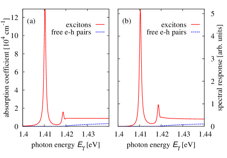
Figure 1: (a) Linear absorption coefficient of a bulk direct gap semiconductor absorber described by two parabolic bands, as computed via the coherent interband polarization function corrected for electron-hole interactions. For comparison, the absorption of non-interacting electron-hole pairs is shown as well. (b) Spectral response for the same system as computed via the effective electron-photon self energy corrected for electron-hole interactions.

Table 1: Material parameters used in the simulations

	$m^{*}_{c}/m_{0}$	$m^{*}_{v}/m_{0}$	$E_{g}$	$\bar{p}_{cv}^{2}/m_{0}$	$\varepsilon$
GaAs	0.067	0.1	1.42 eV	18 eV	13.6
AlxGa1-xAs	0.095	0.1	1.82 eV	18 eV	12.2

The expression for the (singular) interband self-energy may now be rewritten using the above result (33) for the interband Green’s function,

$$\Sigma^{\delta}_{vc}(\mathbf{k},E)= \Sigma^{\delta,e\gamma}_{vc}(\mathbf{k},E)+\Sigma^{\delta,Cb}_{vc}(\mathbf{k},E)$$

$$= \Sigma^{\delta}_{vc,(0)}(\mathbf{k},E)+i\hbar\sum_{\mathbf{q}}V(\mathbf{k}-\mathbf{q})G^{<}_{vc}(\mathbf{q};E)$$

$$= \Sigma^{\delta}_{vc,(0)}(\mathbf{k},E)+\sum_{\mathbf{q}}V(\mathbf{k}-\mathbf{q})\mathcal{T}(\mathbf{q};E)\Sigma^{\delta}_{vc}(\mathbf{q},E),$$ (45)

In order to obtain the Coulomb enhancement factor for the effective interband coupling, the equation is formulated for the normalized self-energy $\sigma^{\delta}_{vc}(\mathbf{k},E)\equiv[\Sigma^{\delta}_{vc,(0)}(E)]^{-1}\Sigma^{\delta}_{vc}(\mathbf{k},E)$, neglecting the quasi-momentum dependence of the momentum matrix elements,

$$\sigma^{\delta}_{vc}(\mathbf{k},E)= 1+\sum_{\mathbf{q}}V(\mathbf{k}-\mathbf{q})\mathcal{T}(\mathbf{q};E)\sigma^{\delta}_{vc}(\mathbf{q},E),$$ (46)

which is idependent of the exciting field an hence related to the macroscopic interband susceptibility. The effective interband self-energy for monochromatic illumination with frequency $\omega_{0}$ can then be written as follows:

$$\tilde{\Sigma}_{cc}^{<,e\gamma}(\mathbf{k};E)= |\Sigma^{\delta}_{cv,(0)}(\hbar\omega_{0})|^{2}|\sigma^{\delta}_{vc}(\mathbf{k},\hbar\omega_{0})|^{2}$$

$$\times\tilde{G}_{vv}^{<}(\mathbf{k};E-\hbar\omega_{0}).$$ (47)

The spectral response displayed in Fig. 1b) is obtained from the photocurrent given by the bulk version of (31),

$$J^{\gamma}(\hbar\omega_{\gamma})= \sum_{\alpha}\int\frac{dE}{2\pi}\sum_{\mathbf{k}}\Big{[}\hbar^{-1}\Gamma^{\alpha}(\mathbf{k};E)\{n_{F}(E-\mu_{\alpha})$$

$$\times A(\mathbf{k};E)+iG^{<}(\mathbf{k};E)\}\Big{]},$$ (48)

where the Coulomb corrections enter via the effective interband self-energy (18) used in the equations for the Green’s functions $G^{\alpha}$, $\alpha=R/A,\lessgtr$.

III.2 Thin films

If periodicity is restricted to the transverse dimensions, Eq. (20) becomes

$$G^{<}_{vc} (\mathbf{k}_{\parallel},z_{1},z_{1}^{\prime};E)=G^{<}_{vc,(0)}(\mathbf{k}_{\parallel},z_{1},z_{1}^{\prime};E)$$

$$+\int dz_{2}\int dz_{3}\mathcal{T}(\mathbf{k}_{\parallel},z_{1},z_{2},z_{3},z_{1^{\prime}};E)$$

$$\times\sum_{\mathbf{q}_{\parallel}}V(\mathbf{k}_{\parallel}-\mathbf{q}_{\parallel},z_{2},z_{3})G^{<}_{vc}(\mathbf{q}_{\parallel},z_{2},z_{3};E),$$ (49)

where $V$ is again the screened Coulomb potential. With the approximation of angular isotropy in the transverse dimensions, the BSE equation may be written

$$G^{<}_{vc} (k_{\parallel},z_{1},z_{1}^{\prime};E)=G^{<}_{vc,(0)}(k_{\parallel},z_{1},z_{1}^{\prime};E)$$

$$+\int dz_{2}\int dz_{3}\mathcal{T}(k_{\parallel},z_{1},z_{2},z_{3},z_{1^{\prime}};E)$$

$$\times\int dq_{\parallel}\tilde{V}(k_{\parallel},q_{\parallel},z_{2},z_{3})G^{<}_{vc}(q_{\parallel},z_{2},z_{3};E),$$ (50)

with the effective, statically screened Coulomb potential

$$\tilde{V}(k_{\parallel},q_{\parallel},z_{1},z_{2})= \frac{e^{2}}{8\pi^{2}\varepsilon\varepsilon_{0}}q_{\parallel}\int_{0}^{2\pi}d\theta~{}\frac{e^{-\tilde{q}(k_{\parallel},q_{\parallel},\theta)|z_{1}-z_{2}|}}{\tilde{q}(k_{\parallel},q_{\parallel},\theta)},$$

$$\tilde{q}(k_{\parallel},q_{\parallel},\theta)\equiv \sqrt{k_{\parallel}^{2}+q_{\parallel}^{2}-2k_{\parallel}q_{\parallel}\cos\theta+q_{0}^{2}}.$$ (51)

Neglecting the short-range contribution of the Bloch functions, the Coulomb-matrix element for a localized real-space basis set may be approximated as $\tilde{V}_{ij}(k_{\parallel},q_{\parallel})\approx\tilde{V}(k_{\parallel},q_{\parallel},z_{i},z_{j})$. Fig. 2 shows the spatial and momentum dependence of the effective, statically screened Coulomb potential for two different values of the inverse screening length, $q_{0}=10^{6}$ m^-1 and $q_{0}=10^{9}$ m^-1, corresponding to the limiting cases of weak and strong screening, respectively. As is to be expected, a small screening length leads to a long-range interaction that is strongly localized in momentum space, with the opposite behavior in the case of large screening length.

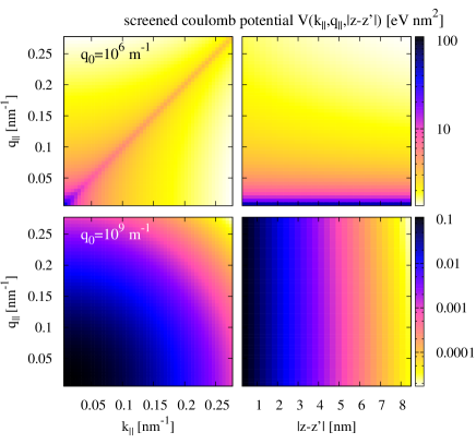
Figure 2: (Color online) Quasi-momentum ($z=z^{\prime}$, left column) and spatial ($q_{\parallel}=k_{\parallel}$, right column) dependence of the statically screened Coulomb interaction for real space resolution in one dimension. In the low-screening limit ($q_{0}=10^{6}$ m^-1, upper row), the interaction is local in momentum space and uniform in real space. In the strong screening regime ($q_{0}=10^{9}$ m^-1, lower row), the situation is reversed.

Using the localized basis representation, the BSE for the coherent interband polarization function may be expressed as a matrix equation in analogy to the bulk case,

$$[G^{<}_{vc}(E)]_{\alpha}=[G^{<}_{vc,0}(E)]_{\alpha}+\sum_{\beta}\tilde{M}_{\alpha\beta}(E)[G^{<}_{vc}(E)]_{\beta},$$ (52)

where multi-index notation is used, with $\alpha=(i,j,k_{\parallel})$ and $\beta=(l,m,q_{\parallel})$, and

$$\tilde{M}_{\alpha(ijk_{\parallel}),\beta(lmq_{\parallel})}(E)=\mathcal{T}_{ilmj}(k_{\parallel};E)\tilde{V}_{lm}(k_{\parallel},q_{\parallel})\Delta q_{\parallel}.$$ (53)

The corresponding equation for the linear susceptibility $\chi$ may be obtained from the above equation

$$[\chi_{vc}(E)]_{\alpha}=[\chi_{vc,(0)}(E)]_{\alpha}+\sum_{\beta}\tilde{M}_{\alpha\beta}(E)[\chi_{vc}(E)]_{\beta},$$ (54)

with $\chi_{vc,(0)}=\mathcal{T}$. This leads to the equation

$$\left[\mathbbm{1}-\tilde{\mathbf{M}}(E)\right]\boldsymbol{\chi}_{vc}(E)=\tilde{\boldsymbol{\chi}}_{vc,(0)}(E),$$ (55)

where

$$[\tilde{\chi}_{vc}(E)]_{\alpha(ijk_{\parallel})}=\sum_{l}\chi_{vc,illj}(k_{\parallel};E).$$ (56)

The expression corresponding to (45) for the self-consistent equation for the singular self-energy reads

$$\Sigma_{vc}^{\delta}(\mathbf{k}_{\parallel},z_{1},z_{1}^{\prime};E) =\Sigma_{vc,(0)}^{\delta}(\mathbf{k}_{\parallel},z_{1},z_{1}^{\prime};E)$$

$$+\sum_{\mathbf{q}_{\parallel}}V(\mathbf{k}_{\parallel}-\mathbf{q}_{\parallel},z_{1}-z_{1}^{\prime})$$

$$\times\int dz_{2}\int dz_{3}\mathcal{T}(\mathbf{q}_{\parallel},z_{1},z_{2},z_{3},z_{1}^{\prime};E)$$

$$\times\Sigma_{vc}^{\delta}(\mathbf{q}_{\parallel},z_{2},z_{3};E).$$ (57)

In the discrete basis, the angular isotropy limit of the above equation is

$$[\Sigma_{vc,(0)}^{\delta}]_{ij}(k_{\parallel};E)= \sum_{lmq_{\parallel}}\Big{[}\delta_{lmq_{\parallel},ijk_{\parallel}}-\tilde{V}_{ij}(k_{\parallel},q_{\parallel})$$

$$\times\mathcal{T}_{ilmj}(q_{\parallel};E)\Big{]}[\Sigma_{vc}^{\delta}]_{lm}(q_{\parallel};E),$$ (58)

which can again be solved via matrix inversion.

In general, the size of the matrices appearing in Eqs. (52) and (58) prohibits the computation of the full matrix. In a first approximation, off-diagonal elements in the spatial indices $(i,j)$ are neglected, the long-range contributions of the electron-hole Coulomb interaction are thus lost, which may lead to an underestimation of the exciton binding energy. The approximation is reasonable in the case of strong screening, especially for the polarization function, where a local interaction removes the second spatial integration. In the equation for the singular self-energy, only the diagonal elements are modified by the Coulomb interaction if the potential is local. In the other extreme of low screening, where the Coulomb potential is spatially constant, one still needs to account for the non-locality of $\mathcal{T}$. In the following numerical examples, the spatial integration over $z_{3}$ in (49) is considered via replacing the interaction potential with the term $\bar{V}(k_{\parallel},q_{\parallel};z_{2})\equiv\int dz_{3}\tilde{V}(k_{\parallel},q_{\parallel};z_{2},z_{3})$. For consistency, the same correction factor is used for the effective potential in (57).

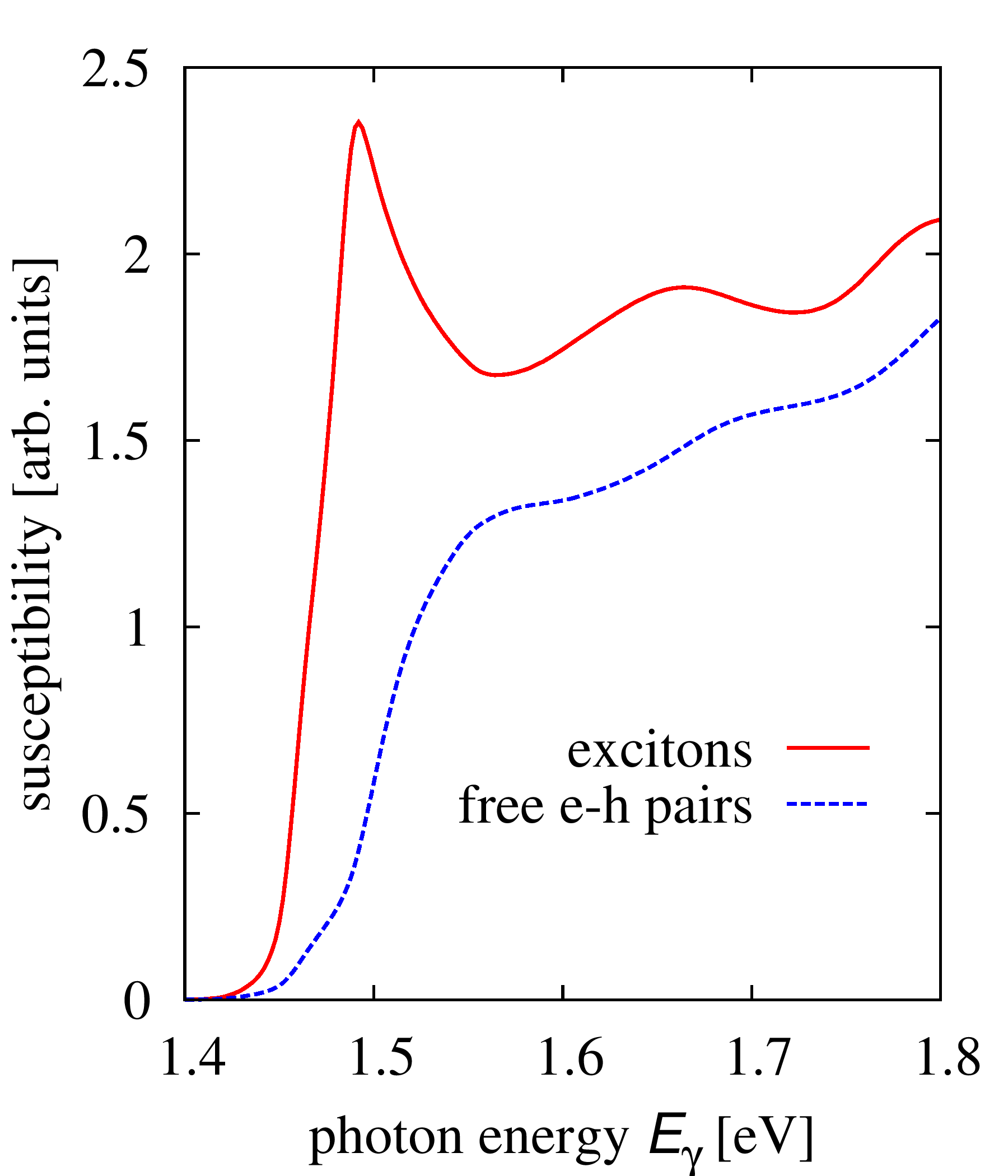
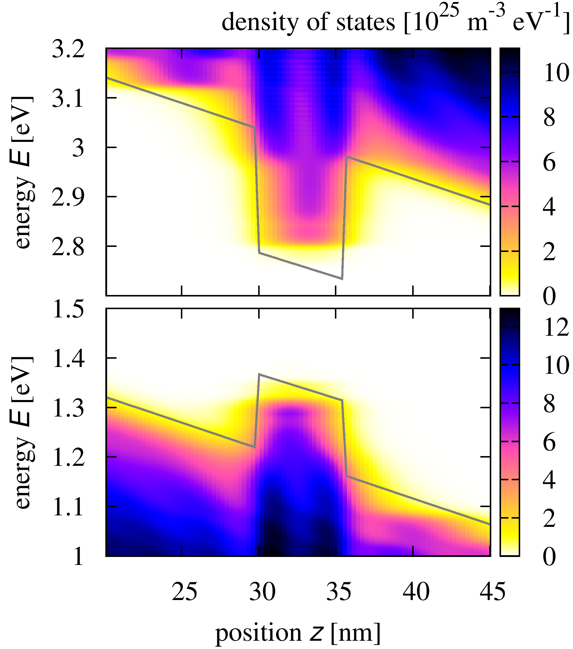
Figure 3: (Color online) a) Coherent excitonic absorption and spectral response of a 5 nm GaAs quantum well embedded in the intrinsic region of a Al_xGa_1-xAs pin diode. b) Local density of states of the same system, revealing the situation at finite field and substantial scattering.

Fig. 3a) shows the effects of the Coulomb correlations on absorption and photocurrent response of a 5 nm wide GaAs quantum well embedded in the center of the intrinsic region of an Al_xGa_1-xAs ($x\sim 0.3$) $p$-$i$-$n$ diode at a contact Fermi level splitting of 1 V and for $q_{0}=10^{6}$ m^-1. The parameters for the bulk materials are given in Tab. 1, and the band offsets are $\Delta E_{c}=0.2$ eV and $\Delta E_{v}=0.15$. The band bending is obtained from self-consistent coupling to Poisson’s equation. Scattering is treated as in Ref. Aeberhard and Morf, 2008. The LDOS of the quantum well region displayed in Fig. 3b) reflects the effects of the sizable built-in field of $\sim 100$ kV/cm and the strong electron-phonon interaction. The corrected susceptibility shows a distinct exciton peak broadened by phonons. The spatially resolved susceptibility in the QW, proportional to the local generation rate, is shown for free-electron hole pairs in Fig. 4a) and for excitons in Fig. 4b). Again, both the appearance of the exciton peaks below the absorption edges of the non-interacting system as well as the enhancement of the quasi-continuum absorption represent the salient features of the correlated transitions.

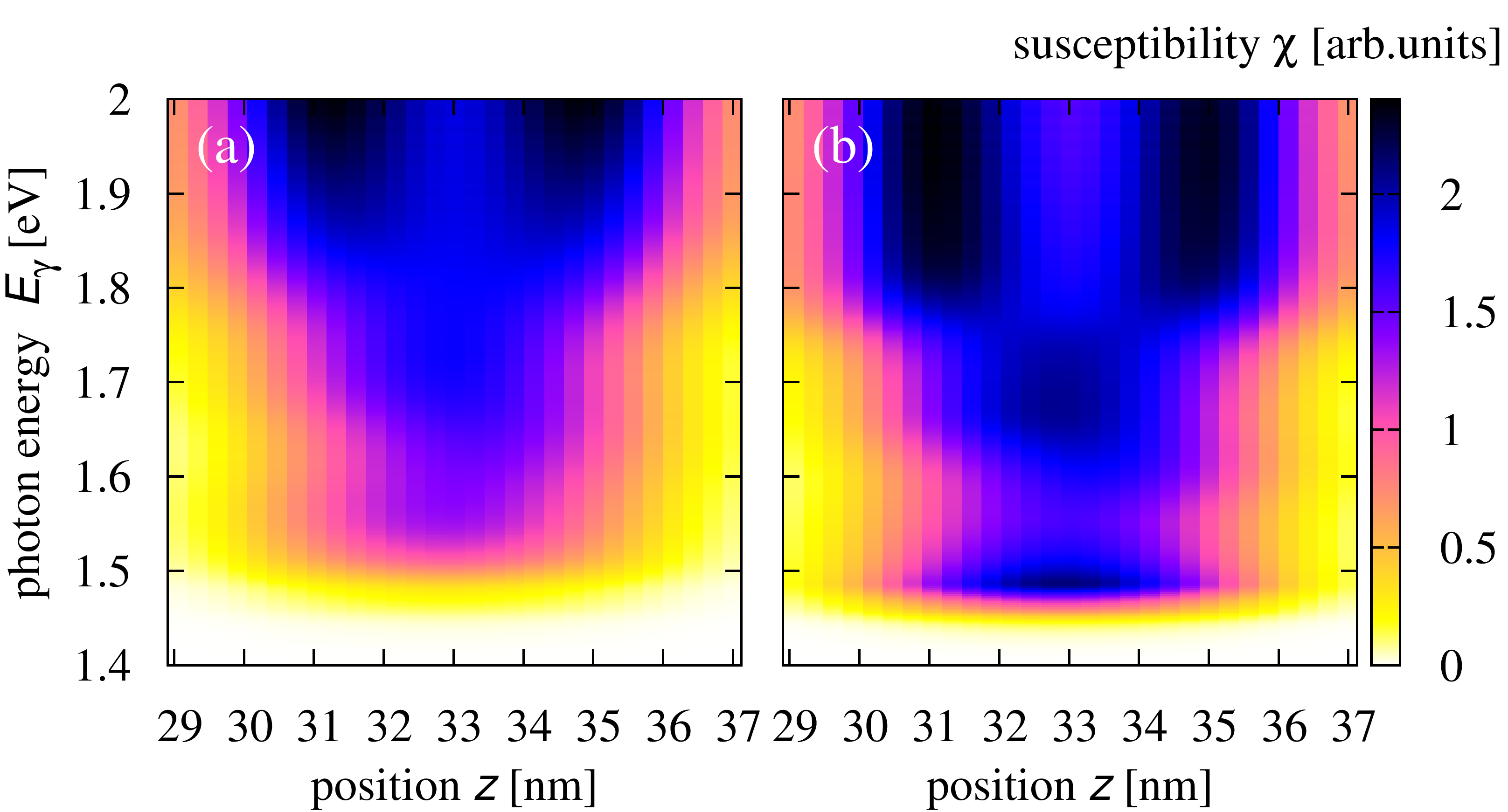
Figure 4: (Color online) a) Coherent local susceptibility in the QW region for the case of non-interacting electron-hole pairs. b) Same for the system with excitonic corrections, exhibiting the salient features of correlated transtions, with exciton peaks broadenend by electron-phonon interaction and an enhancement of the quasi-continuum.

IV Conclusions

In this paper, a consistent inclusion of excitonic effects into the computation of the photocurrent response of photovoltaic nanostructures was presented. While a full treatment of the two particle interactions is still out of range in the context of quantum transport simulations, the excitonic enhancement of the coupling to classical radiation fields can be considered via the corresponding modification of the electron-photon self-energy entering the equations for the charge carrier non-equilibrium Green’s functions. However, since the correlations near the band gap do also have a strong impact on any interband recombination process, it remains desirable to extend the theoretical treatment to incoherent excitons formed by electronically or optically injected carriers.

Appendix A Band decoupling procedure

The standard real-time decomposition rules Langreth (1976) applied to (3) yield the coupled equations for the retarded components of the intra- and interband Green’s functions,

$$G^{-1}_{0,cc}(1,1)G^{R}_{cc}(1,1^{\prime})= \delta(1,1^{\prime})+\int{\mathrm{d}}2\,\Big{[}\Sigma_{cv}^{R}(1,2)G_{vc}^{R}(2,1^{\prime})$$

$$+\Sigma_{cc}^{R}(1,2)G^{R}_{cc}(2,1^{\prime})\Big{]},$$ (59)

$$G^{-1}_{0,vv}(1,1)G^{R}_{vc}(1,1^{\prime})= \int{\mathrm{d}}2\,\Big{[}\Sigma_{vc}^{\delta}(1,2)G_{cc}^{R}(2,1^{\prime})$$

$$+\Sigma_{vv}^{R}(1,2)G^{R}_{vc}(2,1^{\prime})\Big{]}.$$ (60)

Introducing the new quantity

$$\tilde{G}_{vv}^{R}\equiv\left[G^{-1}_{0,vv}-\Sigma_{vv}^{R}\right]^{-1},$$ (61)

in (60), the retarded interband Green’s function can be written as

$$G_{vc}^{R}(1,1^{\prime})=\int{\mathrm{d}}2\int{\mathrm{d}}3\,\tilde{G}_{vv}^{R}(1,2)\Sigma_{vc}^{\delta}(2,3)G_{cc}^{R}(3,1^{\prime}).$$ (62)

Inserting the above expression in (59) provides a closed equation for the retarded intraband Green’s function,

$$G_{cc}^{R}(1,1^{\prime})= \left[G^{-1}_{0,cc}(1,1^{\prime})-\Sigma_{cc}^{R}(1,1^{\prime})-\Sigma_{cc}^{\delta R}(1,1^{\prime})\right]^{-1}$$ (63)

$$\equiv \left[G^{-1}_{0,cc}(1,1^{\prime})-\tilde{\Sigma}_{cc}^{R}(1,1^{\prime})\right]^{-1},$$ (64)

where the contribution from the singular terms to effective band-coupling intra-band self-energy $\tilde{\Sigma}$ is

$$\Sigma_{cc}^{\delta R}(1,1^{\prime})\equiv\int{\mathrm{d}}2\int{\mathrm{d}}3\,\Sigma_{cv}^{\delta}(1,2)\tilde{G}_{vv}^{R}(2,3)\Sigma_{vc}^{\delta}(3,1^{\prime}).$$ (65)

In the same way, the lesser and greater components of the Green’s functions can be decoupled: starting from

$$G^{-1}_{0,cc}(1,1)G^{<}_{cc}(1,1^{\prime})=\int{\mathrm{d}}2\,\left[\Sigma_{cv}^{\delta}(1,2)G_{vc}^{<}(2,1^{\prime})+\Sigma_{cc}^{R}(1,2)G^{<}_{cc}(2,1^{\prime})+\Sigma_{cc}^{<}(1,2)G^{A}_{cc}(2,1^{\prime})\right],$$ (66)

$$G^{-1}_{0,vv}(1,1)G^{<}_{vc}(1,1^{\prime})=\int{\mathrm{d}}2\,\left[\Sigma_{vc}^{\delta}(1,2)G_{cc}^{<}(2,1^{\prime})+\Sigma_{vv}^{R}(1,2)G^{<}_{vc}(2,1^{\prime})+\Sigma_{vv}^{<}(1,2)G^{A}_{vc}(2,1^{\prime})\right].$$ (67)

the interband correlation or coherent polarization function is written as

$$G_{vc}^{<}(1,1^{\prime})= \int{\mathrm{d}}2\,\int{\mathrm{d}}3\,\Big{[}\tilde{G}_{vv}^{R}(1,2)\Sigma_{vc}^{\delta}(2,3)G_{cc}^{<}(3,1^{\prime})$$

$$+\tilde{G}_{vv}^{<}(1,2)\Sigma_{vc}^{\delta}(2,3)G_{cc}^{A}(3,1^{\prime})\Big{]},$$ (68)

where

$$\tilde{G}_{vv}^{<}(1,1^{\prime})\equiv\int{\mathrm{d}}2\int{\mathrm{d}}3\,\tilde{G}_{vv}^{R}(1,2)\Sigma_{vv}^{<}(2,3)\tilde{G}_{vv}^{A}(3,1^{\prime})$$ (69)

was introduced. Replacing the interband term in (66) then yields the intraband correlation function

$$G_{cc}^{<}(1,1^{\prime})= \int{\mathrm{d}}2\int{\mathrm{d}}3\,G_{cc}^{R}(1,2)\Big{[}\Sigma_{cc}^{<}(2,3)$$

$$+\Sigma_{cc}^{\delta<}(2,3)\Big{]}G_{cc}^{A}(3,1^{\prime})$$ (70)

$$\equiv \int{\mathrm{d}}2\int{\mathrm{d}}3\,G_{cc}^{R}(1,2)\tilde{\Sigma}_{cc}^{<}(2,3)G_{cc}^{A}(3,1^{\prime})$$ (71)

with

$$\Sigma_{cc}^{\delta<}(1,1^{\prime})\equiv\int{\mathrm{d}}2\int{\mathrm{d}}3\,\Sigma_{cv}^{\delta}(1,2)\tilde{G}_{vv}^{<}(2,3)\Sigma_{vc}^{\delta}(3,1^{\prime}).$$ (72)

The expressions for the valence band self-energy corrections are obtained from analogous derivations as and are identical to the above result with $c\leftrightarrow v$.

References

• Ekins-Daukes et al. (1999) N. J. Ekins-Daukes, K. W. J. Barnham, J. P. Connolly, J. S. Roberts, J. C. Clark, G. Hill,  and M. Mazzer, Appl. Phys. Lett., 75, 4195 (1999).
• Green (2000) M. A. Green, J. Mater. Sci. Eng. B, 74, 118 (2000).
• Conibeer et al. (2006) G. Conibeer, M. Green, R. Corkish, Y. Cho, E. C. Cho, C. W. Jiang, T. Fangsuwannarak, E. Pink, Y. D. Huang, T. Puzzer, T. Trupke, B. Richards, A. Shalav,  and K. L. Lin, Thin Solid Films, 511, 654 (2006).
• Martí et al. (2006) A. Martí, N. López, E. Antolín, S. C. Cánovas, E. and, C. Farmer, L.  , Cuadra,  and A. Luque, Thin Solid Films, 511, 638 (2006).
• Aeberhard and Morf (2008) U. Aeberhard and R. H. Morf, Phys. Rev. B, 77, 125343 (2008).
• Aeberhard (2011) U. Aeberhard, Nanoscale Res. Lett., 6, 242 (2011a).
• Aeberhard (2011) U. Aeberhard, J. Comput. Electron., 10, 394 (2011b),.
• Aeberhard (2012) U. Aeberhard, Opt. Quantum. Electron., 44, 133 (2012),.
• Haug and Schmitt-Rink (1984) H. Haug and S. Schmitt-Rink, Prog. Quantum Electron., 9, 3 (1984),.
• Haug and Henneberger (1988) H. Haug and K. Henneberger, Phys. Rev. B, 38, 9759 (1988).
• Haug (1992) H. Haug, Phys. Status Solidi B, 173, 139 (1992).
• Haug and Jauho (1996) H. Haug and A. P. Jauho, Quantum kinetics in transport and optics of semiconductors (Springer, Berlin, 1996).
• Haug and Koch (2004) H. Haug and S. W. Koch, Quantum Theory of the Optical and Electronic Properties of Semiconductors (World Scientific, 2004).
• Henneberger and May (1986) K. Henneberger and V. May, Physica A, 138, 537 (1986).
• Henneberger (1988) K. Henneberger, Physica A, 150, 419 (1988a).
• Henneberger (1988) K. Henneberger, Physica A, 150, 439 (1988b).
• Henneberger and Haug (1988) K. Henneberger and H. Haug, Phys. Rev. B, 38, 9759 (1988).
• Henneberger and Koch (1996) K. Henneberger and S. W. Koch,  Phys. Rev. Lett., 76, 1820 (1996).
• Jahnke and Koch (1995) F. Jahnke and S. W. Koch,  Phys. Rev. A, 52, 1712 (1995).
• Note (1) The description of spontaneous emission would require the additional coupling to an incoherent internal photon field..
• Kadanoff and Baym (1962) L. P. Kadanoff and G. Baym, Quantum Statistical Mechanics (Benjamin, Reading, Mass., 1962).
• Keldysh (1965) L. Keldysh, Sov. Phys. JETP, 20, 1018 (1965).
• Langreth (1976) D. Langreth, in Linear and Non-linear Electron Transport in solids17, 3 (1976).
• Aeberhard (2011) U. Aeberhard, Phys. Rev. B, 84, 035454 (2011c).
• Schäfer and Wegener (2002) W. Schäfer and M. Wegener, Semiconductor Optics and Transport Phenomena (Springer, Berlin, 2002).
• Meir and Wingreen (1992) Y. Meir and N. Wingreen, Phys. Rev. Lett., 68, 2512 (1992).